Embed Size (px)
Citation preview
Valuation of Electricity Futures: Reduced-Form vs.
Dynamic Equilibrium Models
Wolfgang Buhler and Jens Muller-Merbach∗
May 2009
Abstract
Equilibrium and reduced-form models are partly competing, partly complementaryapproaches to value electricity futures. We present the first empirical comparison of aone-factor reduced-form model and a demand driven dynamic equilibrium model. Thecontribution to the literature is twofold. First, on the theoretical side we develop adynamic generalization of the static model by Bessembinder and Lemmon. As a resultwe endogenously derive the term structure of futures prices and risk premia. Second,on the empirical side we test both models using price data from Nord Pool. Our mainfindings are as follows. (1) The equilibrium model is able to explain the increasingvolatility and right-skewness of futures prices for a decreasing time to maturity. (2)The cost function in the equilibrium model has to be parameterized by the waterreservoir level to obtain reasonable spot and futures prices. (3) The equilibrium modelprovides better out-of-sample estimates of futures prices than the reduced-form model,and it is able to capture price peaks.
JEL classification: G13
Keywords: Electricity futures, risk premia, reduced-form models, equilibrium models.
∗Wolfgang Buhler: Chair of Finance, University of Mannheim, D-68131 Mannheim, Germany,[email protected]. Jens Muller-Merbach: BHF-Bank AG, Neue Mainzer Straße 74, 60311 Frank-furt, [email protected]. Financial support from the Deutsche Forschungsgemeinschaft(DFG), Bonn, is gratefully acknowledged.

1 Introduction 1
1 Introduction
The valuation of electricity futures is still a challenging topic. The non-storability of electric-
ity results in two major consequences: First, spot prices exhibit seasonal patterns, a large
volatility, and price peaks. Second, electricity futures cannot be evaluated by the cost-of-
carry approach, and their prices contain risk premia on top of the expected spot price, cf.
Geman (2005, p. 270). Determining these risk premia is a major theoretical and empirical
challenge.
Two approaches have been proposed to price electricity futures: Reduced-form and equilib-
rium models. The advantages and shortcomings of these competing as well as complementary
model classes are well known. Reduced-form models are flexible and parsimonious with re-
gard to the number and the stochastic properties of the risk factors. If modeled suitably,
they allow for closed-form solutions of futures prices. For typical reduced-form models we
refer to Pilipovic (1997), Geman and Vasicek (2001), Koekebakker and Ollmar (2005), Audet
et al. (2002), Lucia and Schwartz (2002), Villaplana (2003), Geman and Roncoroni (2006),
and Cartea and Figueroa (2005).
Equilibrium models focus on modeling the production and demand structure of electricity.
Spot and futures prices, risk premia and their properties are determined endogenously. In
their fundamental dynamic model, Routledge et al. (2001) derive their pricing results by
explicitly considering also the storage possibilities of different types of fuel and its sequen-
tial conversion into electricity. In the static model by Bessembinder and Lemmon (2002)
hedging activities of risk-averse electricity producers and retailers drive the futures prices.
Ullrich (2007) adds capacity constraints to the Bessembinder/Lemmon-model. Benth et al.
(2007) use a time-dependent allocation of market power between risk-averse producers and
consumers to receive futures prices in equilibrium that may contain positive or negative risk
premia.
Our model contributes to the literature in the following ways. On the theoretical side we
derive a dynamic generalization of the static model by Bessembinder and Lemmon. This
dynamic version has several important features. First, it endogenously generates the term
structure of futures prices and its risk premia. Comparative statics show that the dynamic
approach can explain increasing, decreasing, and hump-shaped term structures of risk premia

1 Introduction 2
even when there is no seasonal structure in the prices. Second, it explains empirical stochastic
characteristics as the increasing volatility and right-skewness of futures prices for decreasing
time to maturity. Third, the dynamic setting is necessary to evaluate cascading futures as
they are common at most electricity exchanges. For a more detailed derivation we refer to
Buhler and Muller-Merbach (2008).
On the empirical side we present the first study that compares a reduced-form and our
equilibrium pricing model for electricity futures. Both models use one exogenous factor,
the spot price and the demand for electricity, respectively, which shows a strong seasonal
pattern. We use the best performing one-factor reduced-form model in the study by Lucia
and Schwartz (2002). In the equilibrium model, additional to the stochastic demand, the
cost structure of the producers and the changing level of the water reservoir matter for the
spot and futures prices.
We conduct our empirical analysis with data from the Scandinavian exchange Nord Pool.
Nord Pool provides, in addition to price data, also time series of the end-user demand and
of the water reservoir level. We test and compare the two models with weekly observations
of futures prices during a period of 50 months. This period contains years with a rather low
volatility, but also times with a record level of prices and large price jumps.
Our main empirical findings are as follows. Assuming risk-neutral agents as a benchmark we
find that the equilibrium model provides better out-of-sample futures price estimates than
the reduced-form model. The absolute mean estimation error, the standard deviation, and
the maximum of the estimation errors are lower for this model. The result can be traced back
to the following reasons. (1) The reduced-form model shows a reasonable performance during
calm price periods. It is, however, not able to capture price peaks in an appropriate way.
These peaks are properly reflected in the equilibrium model as the cost function depends
on the water reservoir level. This variable is highly correlated with spot and futures prices.
(2) The spot prices in the reduced-form model are symmetrically distributed, whereas in
the equilibrium model normally distributed demand residuals are transformed by the convex
cost function into skewed spot prices. (3) The seasonal component of the exogenous spot
price in the reduced-form model is harder to estimate than the seasonal component of the
demand. Both models, however, underestimate on average the futures prices. This result
shows that there exist risk premia in futures prices. These premia are positive, i.e. the seller
2 Review of the Models 3
of a futures contract earns on average a surplus. This finding confirms the empirical results
by Longstaff and Wang (2004) and Geman and Vasicek (2001).
The implicit estimation of the market price of risk for the reduced-form model and the
normalized risk aversion parameter in the equilibrium model shows the expected signs. The
market price of risk is on average negative, contrary to the results reported by Lucia and
Schwartz (2002), and the normalized risk aversion parameter has a positive sign.
On average, the out-of-sample pricing errors of both models are reduced if the implicitly
estimated risk parameters are considered in estimating futures prices. Also, the standard
deviation of the pricing errors in the equilibrium model declines, but not for the reduced-form
model. Again, this result is due to the huge pricing error of this model during highly volatile
spot price periods. The analysis of the estimated risk premia shows that the theoretical term
structure of these premia is supported by the observed term structure for the equilibrium
model, but not for the reduced-form approach.
Our paper is organized as follows. Section 2 shortly reviews the two models. Section 3 de-
scribes the spot and futures market at Nord Pool and Section 4 provides descriptive statistics
for the used time series. In Section 5 we explain the estimation design and procedure. We
present the empirical results in Section 6. Section 7 concludes.
2 Review of the Models
In this section we shortly review the proposed models. For a more detailed description we
refer to the original papers.
2.1 The Reduced-Form Model by Lucia and Schwartz
In their paper, Lucia and Schwartz (2002) propose two different one-factor models as well
as two different two-factor models. Apart from the number of factors the approaches differ
whether the spot price or the log-spot price is used as an exogenous variable. In their em-
pirical study, Lucia and Schwartz find that the spot-price model outperforms the competing
model. Therefore, we restrict our analysis to their spot price model which is shortly reviewed
below.
2 Review of the Models 4
The spot price Pt equals the sum of a deterministic (seasonal) component f(t) and a stochas-
tic component Xt that follows an Ornstein-Uhlenbeck process
dXt = −κXtdt + σXdZt, (1)
where Zt is a Wiener process. σX > 0 denotes the constant volatility and κ > 0 the speed
of adjustment.
Assuming a constant market price of risk, λ, the futures price under the risk-neutral measure
(denoted by ∗) equals the expected spot price at the futures maturity date T . Since Pt =
f(t) + Xt, the futures price Ft,T at date t reads:
Ft,T = E∗t{PT} = f(T ) + (Pt − f(t))e−κ(T−t) − λσX
κ(1− e−κ(T−t)). (2)
The futures price in (2) consists of three additive components. The first one, f(T ), describes
the unconditionally expected future spot price. The second component, (Pt−f(t))e−κ(T−t), is
the difference between the current spot price and its deterministic component. This difference
is discounted with the speed of adjustment κ and reflects the mean-reverting behavior: The
best forecast is to expect that the actual deviation of the spot price from f(t) continuously
fades out. Finally, the third component corrects for the spot price risk. This component is
monotonous in the time-to-maturity and proportional to the market price of risk, λ. The
second and the third term in (2) can be positive or negative.
2.2 The Dynamic Equilibrium Model
In Buhler and Muller-Merbach (2008) we develop a multi-period extension of the static model
by Bessembinder and Lemmon (2002). The general framework of this equilibrium model is
outlined in Section 2.2.1. It has several degrees of freedom that we specify in Section 2.2.2.
2.2.1 Model Framework
The market structure is characterized by competitive, risk-averse producers G and retailers R
of electricity. Both groups are aggregated to two representative agents. We assume that they

2 Review of the Models 5
maximize their terminal wealth WΘ at the planing horizon Θ in a mean-variance framework:
Et{WAΘ } − 1
2λAVart{WA
Θ } , A ∈ {G,R} . (3)
The terminal wealth is determined by the cash flows that the representative agents receive
from producing or retailing electricity, respectively, as well as from their trading activities.
Both agents must trade in the spot market to satisfy the exogenous end-user demand Dt at
each date t. As electricity is not storable, the demand is equal to the production volume.
When not hedged, the producer receives at date t the cash flow
C ′t(Dt)Dt − Ct(Dt). (4)
Ct(D) denotes the variable production cost as a (possibly time-varying) function of the pro-
duced quantity of electricity, D. C ′t(D) denotes the marginal cost function. In a competitive
equilibrium marginal costs equal the spot price. We assume that C ′t is strictly increasing in
the production volume.
The retailer receives the cash flow
pDt − C ′t(Dt)Dt. (5)
p represents the fixed end-user price per unit of electricity which is assumed to be independent
of the consumed quantity of electricity.
By trading futures, both representative agents can change the risk-return position of their
cash flows in (4) and (5), and, by compounding the marking-to-market consequences to the
planning horizon Θ, their terminal wealth WΘ. Solving (3) under the condition of market
clearing determines the futures prices in equilibrium. As discussed in Basak and Chabakauri
(2007), two solution concepts are available. The global solution is not time-consistent and
its implementation needs a commitment device. In Buhler and Muller-Merbach (2008) we
consider the time-consistent solution by dynamic programming which leads to the following

2 Review of the Models 6
equilibrium futures prices:
Ft,T = Et{Ft+1,T} − ξ
Θ∑
θ=t+1
er(Θ−θ)Covt{pDθ − Cθ(Dθ); Ft+1,T} , t < T ≤ Θ, (6)
where ξ = λRλG
λR+λG is the combined risk aversion factor and r the constant interest rate. In
the last period before maturity, (6) can be written as
FT−1,T = ET−1{FT,T}−ξ
Θ∑
θ=T−1
er(Θ−θ)CovT−1{pDθ−Cθ(Dθ); C′T (DT )} , t < T ≤ Θ, (7)
where FT,T = C ′T (DT ) is the final settlement price and equals the spot price PT . Note that
(6) represents equilibrium futures prices recursively only.
The equilibrium futures price in (6) is equal to the expected next period’s futures price
or spot price, respectively, minus a risk premium. This risk premium is the sum of the
covariances between future cash flows and the next period’s endogenous futures or spot
price. The term pDθ−Cθ(Dθ) denotes the aggregate net cash flow that the whole electricity
sector receives in the economy. The representative retailer receives pDt and the producer
has to pay Ct(Dt) for the production during the time interval [t, t + 1). The spot and the
futures market allocate the aggregate cash flow and the cash flow risk between the producer
and the retailer.
2.2.2 Model Specification
Two factors in the equilibrium model are yet to be specified: The process of the state variable,
i. e. the end-user demand Dt, and the cost structure. We assume that the stochastic process
of Dt is the sum of a deterministic component Dt and a stochastic component St. Dt reflects
the characteristic seasonal patterns. The functional form of Dt that we use in the empirical
analysis is described in Appendix A. The stochastic component St is modeled as a first-order
autoregressive process:
St = ρSt−1 + σS εSt , εS
t ∼ N (0, 1) i.i.d. (8)
2 Review of the Models 7
0
100
200
300
400
500
600
-10 0 10 20 30 40 50 60
D*
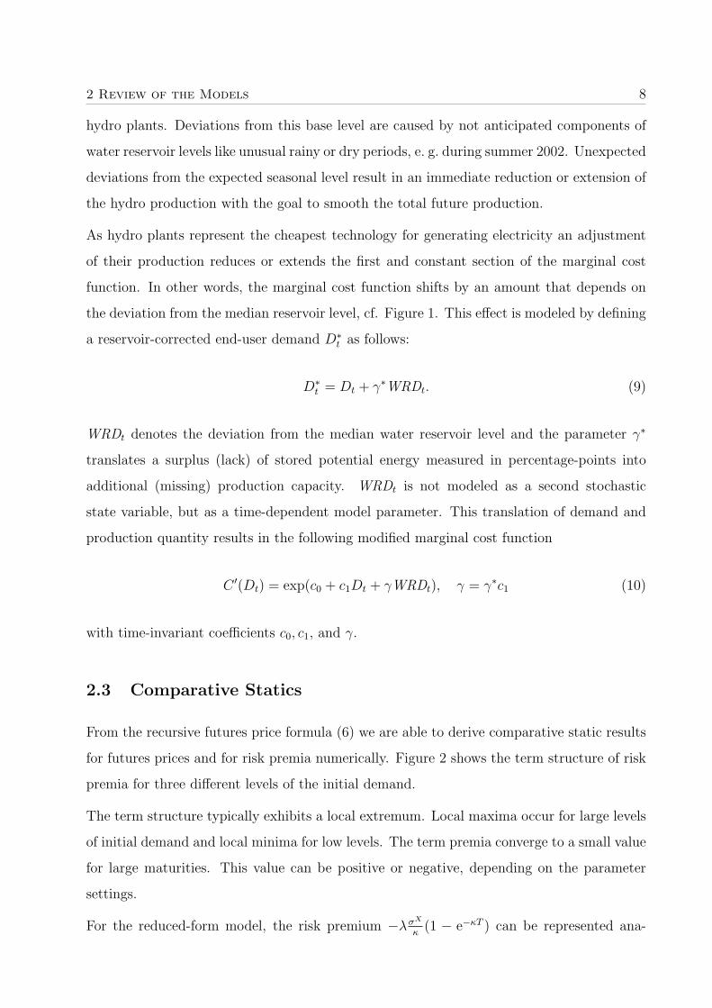
Hydro-generated electricity if the reservoir level is larger than the median.
Hydro-generated electricity if the resevoir level is
smaller than the median.
Hydro-generated electricity if the reservoir level equals the median.
DD0 10 200
C' [NOK/MW]
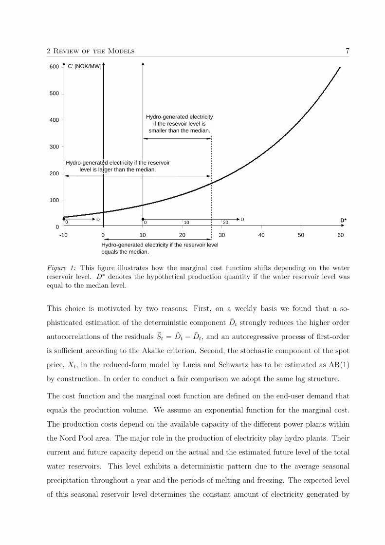
Figure 1: This figure illustrates how the marginal cost function shifts depending on the waterreservoir level. D∗ denotes the hypothetical production quantity if the water reservoir level wasequal to the median level.
This choice is motivated by two reasons: First, on a weekly basis we found that a so-
phisticated estimation of the deterministic component Dt strongly reduces the higher order
autocorrelations of the residuals St = Dt − Dt, and an autoregressive process of first-order
is sufficient according to the Akaike criterion. Second, the stochastic component of the spot
price, Xt, in the reduced-form model by Lucia and Schwartz has to be estimated as AR(1)
by construction. In order to conduct a fair comparison we adopt the same lag structure.
The cost function and the marginal cost function are defined on the end-user demand that
equals the production volume. We assume an exponential function for the marginal cost.
The production costs depend on the available capacity of the different power plants within
the Nord Pool area. The major role in the production of electricity play hydro plants. Their
current and future capacity depend on the actual and the estimated future level of the total
water reservoirs. This level exhibits a deterministic pattern due to the average seasonal
precipitation throughout a year and the periods of melting and freezing. The expected level
of this seasonal reservoir level determines the constant amount of electricity generated by
2 Review of the Models 8
hydro plants. Deviations from this base level are caused by not anticipated components of
water reservoir levels like unusual rainy or dry periods, e. g. during summer 2002. Unexpected
deviations from the expected seasonal level result in an immediate reduction or extension of
the hydro production with the goal to smooth the total future production.
As hydro plants represent the cheapest technology for generating electricity an adjustment
of their production reduces or extends the first and constant section of the marginal cost
function. In other words, the marginal cost function shifts by an amount that depends on
the deviation from the median reservoir level, cf. Figure 1. This effect is modeled by defining
a reservoir-corrected end-user demand D∗t as follows:
D∗t = Dt + γ∗WRDt. (9)
WRDt denotes the deviation from the median water reservoir level and the parameter γ∗
translates a surplus (lack) of stored potential energy measured in percentage-points into
additional (missing) production capacity. WRDt is not modeled as a second stochastic
state variable, but as a time-dependent model parameter. This translation of demand and
production quantity results in the following modified marginal cost function
C ′(Dt) = exp(c0 + c1Dt + γWRDt), γ = γ∗c1 (10)
with time-invariant coefficients c0, c1, and γ.
2.3 Comparative Statics
From the recursive futures price formula (6) we are able to derive comparative static results
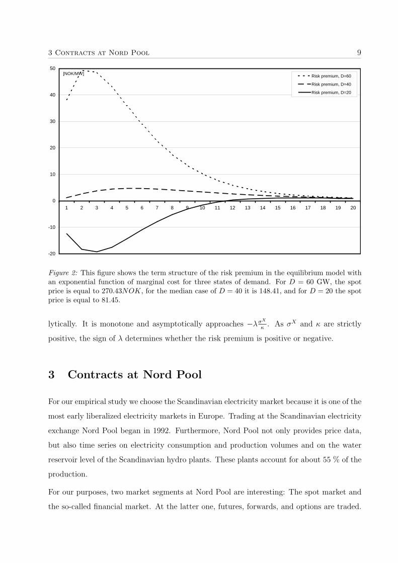
for futures prices and for risk premia numerically. Figure 2 shows the term structure of risk
premia for three different levels of the initial demand.
The term structure typically exhibits a local extremum. Local maxima occur for large levels
of initial demand and local minima for low levels. The term premia converge to a small value
for large maturities. This value can be positive or negative, depending on the parameter
settings.
For the reduced-form model, the risk premium −λσX
κ(1 − e−κT ) can be represented ana-
3 Contracts at Nord Pool 9
-20
-10
0
10
20
30
40
50
1 2 3 4 5 6 7 8 9 10 11 12 13 14 15 16 17 18 19 20
Risk premium, D=60
Risk premium, D=40
Risk premium, D=20
[NOK/MW]
Figure 2: This figure shows the term structure of the risk premium in the equilibrium model withan exponential function of marginal cost for three states of demand. For D = 60 GW, the spotprice is equal to 270.43NOK, for the median case of D = 40 it is 148.41, and for D = 20 the spotprice is equal to 81.45.
lytically. It is monotone and asymptotically approaches −λσX
κ. As σX and κ are strictly
positive, the sign of λ determines whether the risk premium is positive or negative.
3 Contracts at Nord Pool
For our empirical study we choose the Scandinavian electricity market because it is one of the
most early liberalized electricity markets in Europe. Trading at the Scandinavian electricity
exchange Nord Pool began in 1992. Furthermore, Nord Pool not only provides price data,
but also time series on electricity consumption and production volumes and on the water
reservoir level of the Scandinavian hydro plants. These plants account for about 55 % of the
production.
For our purposes, two market segments at Nord Pool are interesting: The spot market and
the so-called financial market. At the latter one, futures, forwards, and options are traded.

3 Contracts at Nord Pool 10
All prices used in our study are given in NOK/MW.1 In the spot market electricity is traded
for physical delivery during each single hour of the subsequent day (or days, if weekends or
exchange holidays follow). This market is organized as a single auction market. All traders
have to provide their buy or sell offers for each hour of the subsequent day. Nord Pool then
calculates 24 hourly market clearing prices. The equally weighted average of those prices is
called the system price which we refer to as the daily spot price hereafter.
In the financial market forwards and futures are traded continuously. The underlying of all
contracts is the 24-hour-delivery of electricity per day at a constant rate during a specified
delivery period. All contracts are cash settled. The delivery periods of the listed contracts
range from one day to one year. Futures are used for shorter delivery periods, forward
contracts are listed for delivery periods of one month and longer. The time-to-maturity of
the listed contracts, i. e. the time until the delivery period begins, ranges from two days up to
three years. In detail, the following contracts are listed or were listed during our observation
period:
• Day futures with a delivery period of one day are listed with a time-to-maturity between
two and a maximum of ten days. These contracts show a rather low liquidity.
• Week futures have a delivery period from Monday through Sunday and a time-to-
maturity up to eight weeks. They are the most actively traded contracts at Nord Pool,
however, liquidity decreases with increasing time-to-maturity.
• Block futures cover a delivery period of four weeks. The listed maturities comprise the
time interval from eight up to 48 weeks. Block futures were actively traded but were
successively replaced by moth forwards in 2003.
• Month forwards were introduced in 2003. Their delivery periods equal the calendar
months, i. e. 28 to 31 days. The listed maturities cover the subsequent six months.
• For longer delivery periods, quarter, season, and year forwards are or were traded at
Nord Pool. These contracts are the least liquid ones, sometimes only one trade per
week is documented.
1Between 2003 and 2006, Nord Pool subsequently switched from NOK to Euro.
4 Descriptive Statistics 11
Some of these contracts have a special cascade feature that is not found in other commodity
markets. A certain time before maturity they are split up into into a volume-equivalent
bundle of contracts with shorter maturities. In detail, block futures are split into the corre-
sponding four week futures contracts eight weeks before its delivery period begins. For the
longer maturities, year forwards were split into season forwards and are nowadays split into
quarter forwards that in turn are split into month forwards.2 This cascade structure allows
the market participants to hedge their exposures more precisely for closer maturities. Note
that forward contracts are not split into futures.
The financial market Nord Pool only provides so-called closing prices that are used for
the daily settlement of futures. The closing price is the last registered trading price at a
randomly chosen point in time within the last ten minutes of trading.3 If there are no trades
at a certain exchange day, Nord Pool uses several procedures to estimate a closing price. As
Nord Pool also provides the daily trading volumes for each contract, we can identify closing
prices that are based on trading.
4 Descriptive Statistics
Nord Pool published daily spot prices since 1992. However, we do not use spot prices before
11/01/1996, however, because Finish electricity firms gained access to Nord Pool in October
1996.4 The available times series of daily production, consumption, import, and export
volumes start at 03/29/1999.5 The water reservoir level and its deviation from the historical
median are measured once a week and are available since 1996, daily futures prices and
trading volumes since 1995. We only consider transaction prices and not prices that were
set by Nord Pool for settlement purposes only.
For the fixed tariff rate p in the equilibrium model we use the average price of a “1-year/new
fixed-price contracts” for households and industrial customers. This price is provided as a
quarterly time series by Statistics Norway. For the interest rate r we use the 3-month-NIBOR
(Norwegian Interbank Offered Rate) provided by the central bank of Norway.
2The types and the cascade structure of the listed derivatives at Nord Pool are subject to current changes.3See Nord Pool ASA (ed.) (2004) for details.4Nord Pool ASA (ed.) (1998), p. 9.5Prior to that date, the referred time series were available for only some of the countries.
4 Descriptive Statistics 12
All time series end on 08/04/2004. This provides us with a period of 64 months for the
shortest time series, the production and consumption volumes. As we need a period of over
one year to estimate the parameters of the models, we test both models for a period of 50
months from 05/24/2000 to 08/04/2004 (cf. Section 5 for details).
4.1 Daily Spot Prices
In this section we present descriptive statistics of daily spot prices, daily demand, and
the weekly measured water reservoir level for the 64-months period from 03/29/1999 until
08/04/2004. Quantities will be given in GW, prices in NOK/MW if not denoted otherwise.
Figure 5 in the Appendix plots the level of the daily spot price and its first difference during
the five-year period and Table 1 shows the corresponding descriptive statistics. As mentioned
before, the spot price exhibits some seasonality in that the prices during the winter time
are usually higher than in the preceding summer. However, this seasonality is superimposed
by strong changes in the mean level of the spot price. Table 1 shows that in the last two
12-month periods of our observation period the yearly mean as well as the median were
about twice as high as in earlier periods. We also observe a fluctuating standard deviation.
The rather high values for the kurtosis in combination with the mostly positive skewness
reflect the occasional spikes in the spot price process. The price spikes usually occur in the
winter time. In Figure 5 we marked two examples of single spikes, A and B, and a period of
high prices and frequent spikes, C. Spikes A (387.78 NOK/MW) and B (633.36 NOK/MW)
happened on 01/24/2000 and 02/05/2001, respectively, and disappeared one day later. They
are caused by an exceptionally large electricity demand on those two days. This can be seen
in Figure 6 that plots the daily demand volumes.
The third example, C, covers a period of about four months of record high prices that cannot
be explained by demand alone. We argue that these large spot prices are caused by unusually
low water reservoir levels. The period of low precipitation began in summer 2002. Figure 8
shows that during this period the water reservoir deviation from the long term median is
negative and decreasing. As a consequence the production capacity of hydro plants was
reduced and producers were forced to run plants with higher variable costs.6 This period
6Cf. Bye (2003) for a detailed analysis of this period in Norway.

4 Descriptive Statistics 13
01.04.97– 01.04.98– 01.04.99– 01.04.00– 01.04.01– 01.04.02– 01.04.03– whole31.03.98 31.03.99 31.03.00 31.03.01 31.03.02 31.03.03 31.03.04 sample
Daily Spot Price, Pt [NOK/MW]
Obs. 365 365 366 365 365 365 366 2841
Mean 130.27 110.52 108.98 125.33 178.08 258.84 252.70 171.39Std. dev. 29.14 31.69 30.37 60.11 27.15 162.99 33.23 90.45Skewness −0.018 −0.202 2.381 2.511 0.710 1.399 −0.388 2.378Kurtosis −0.29 1.24 19.12 15.22 2.40 1.65 1.20 10.47
Minimum 58.21 21.27 50.43 31.85 119.07 80.65 128.91 21.27Maximum 234.25 266.47 387.78 633.36 335.80 831.41 343.25 831.41
Daily Spot Price Differences, Pt − Pt−1 [NOK/MW]
Obs. 365 365 366 365 365 365 366 2840
Mean 0.04 −0.07 0.03 0.26 −0.22 0.33 0.02 0.00Std. dev. 10.09 11.23 20.02 37.50 17.40 19.66 16.42 20.09Skewness 0.750 −0.599 3.920 3.156 1.722 −0.223 0.964 3.358Kurtosis 3.54 21.12 111.60 66.41 18.82 6.71 4.77 121.88
Minimum −42.02 −96.44 −197.32 −264.29 −98.79 −95.92 −55.65 −264.29Maximum 45.58 76.81 265.49 440.59 151.74 94.00 89.03 440.59
Table 1: Descriptive statistics for the daily spot price Pt and its first differences at Nord Pool inperiod between 11/01/1996 and 08/10/2004 and for subperiods of 12 months each.
will be a challenge for both models.
The high absolute values of the minimum and maximum in Table 1 are an obvious con-
sequence of the price spikes. The high kurtosis and the mostly positive skewness do not
support the assumption of normal distribution. However, note that the values in Table 1
reflect also the seasonal patterns in the spot prices. We will discuss the distribution of spot
prices without the deterministic (seasonal) component in Section 6.
We tested the spot price series for unit roots with the Augmented Dickey-Fuller (ADF) test,
including a constant. With a test value of −3.007 the hypothesis of a unit root is rejected on
the 5%-level if we include up to 35 lags. However, in four out of 217 estimation periods we
found a unit root in the spot price series after having extracted the deterministic components
on a weekly basis (cf. Section 6.2).
4 Descriptive Statistics 14
all week blockfutures futures futures W1 W2 W3 W4 W5 W6 W7 W8
Obs. 5121 2258 2863 406 406 405 399 300 208 114 20
Mean 3.70 8.84 −0.36 4.26 7.04 8.50 9.06 10.61 13.10 14.87 36.05Std. dev. 67.38 48.47 78.95 24.21 39.98 47.20 53.86 59.20 60.93 64.02 51.96Skewness −1.416 3.462 −2.111 5.168 4.333 4.114 3.610 2.260 2.704 2.186 0.450Kurtosis 15.27 35.44 9.43 54.61 45.27 42.30 36.09 24.92 19.64 16.16 −1.52
B1 B2 B3 B4 B5 B6 B7 B8 B9 B10 B11
Obs. 352 348 340 327 318 301 271 238 191 120 57
Mean 6.55 5.26 2.27 0.27 −1.03 −3.62 −5.28 −4.55 −2.37 −5.67 −16.62Std. dev. 65.19 74.88 78.06 79.87 76.22 76.89 83.63 86.44 82.86 91.54 104.91Skewness −0.084 −0.996 −1.857 −2.299 −2.744 −2.757 −2.610 −2.409 −2.162 −2.147 −2.324Kurtosis 11.48 11.73 10.20 9.38 10.56 9.98 8.54 7.55 6.99 6.28 5.27
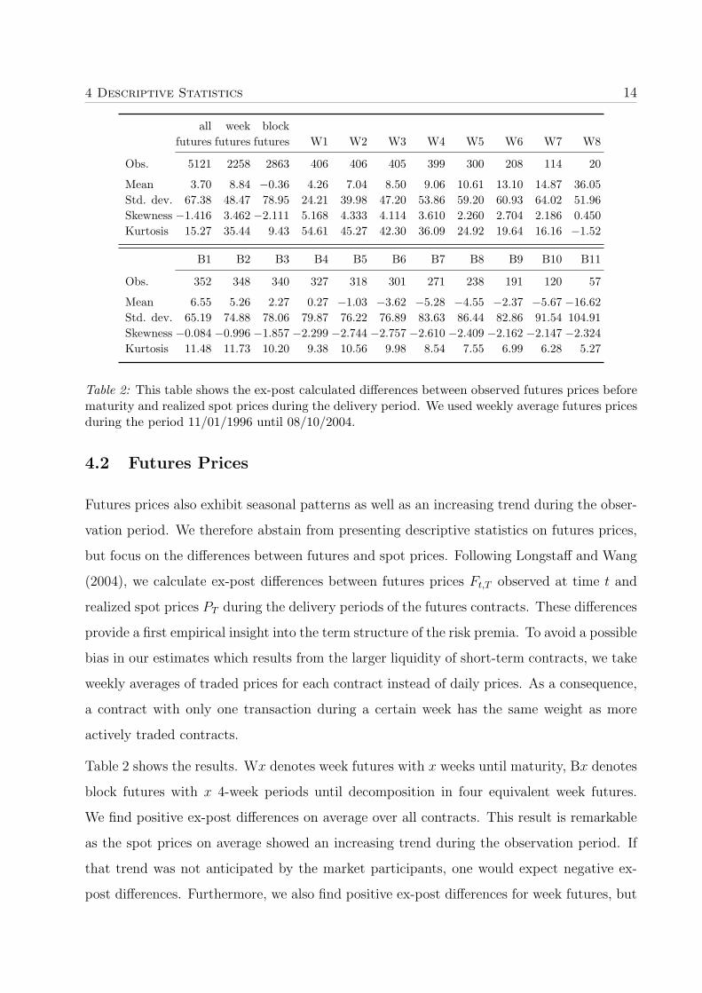
Table 2: This table shows the ex-post calculated differences between observed futures prices beforematurity and realized spot prices during the delivery period. We used weekly average futures pricesduring the period 11/01/1996 until 08/10/2004.
4.2 Futures Prices
Futures prices also exhibit seasonal patterns as well as an increasing trend during the obser-
vation period. We therefore abstain from presenting descriptive statistics on futures prices,
but focus on the differences between futures and spot prices. Following Longstaff and Wang
(2004), we calculate ex-post differences between futures prices Ft,T observed at time t and
realized spot prices PT during the delivery periods of the futures contracts. These differences
provide a first empirical insight into the term structure of the risk premia. To avoid a possible
bias in our estimates which results from the larger liquidity of short-term contracts, we take
weekly averages of traded prices for each contract instead of daily prices. As a consequence,
a contract with only one transaction during a certain week has the same weight as more
actively traded contracts.
Table 2 shows the results. Wx denotes week futures with x weeks until maturity, Bx denotes
block futures with x 4-week periods until decomposition in four equivalent week futures.
We find positive ex-post differences on average over all contracts. This result is remarkable
as the spot prices on average showed an increasing trend during the observation period. If
that trend was not anticipated by the market participants, one would expect negative ex-
post differences. Furthermore, we also find positive ex-post differences for week futures, but

4 Descriptive Statistics 15
differences close to zero for block futures. For week futures the difference increases with the
maturity.
We observe positive, but decreasing ex-post differences for the first four block futures and
slightly negative ones for the block futures with longer times to maturity. Note that there are
only few observations for the W8 and the B11 contract. These differences can be understood
as estimates of the risk premium. Therefore, our results support, basically, the term structure
of risk premia as derived in the equilibrium model.
The standard deviation of the ex-post differences increases with maturity. This observation
reflects the increasing forecasting uncertainty and results in insignificant ex-post differences
for the block futures. Applying a t-test with Newey/West correction shows that only the ex-
post differences for the W1, W2, W3, W6, and W7 contracts are significant at the 5%-level.
4.3 Daily Electricity Production and Demand
For the equilibrium model we need the total electricity consumption or production in the
Nord Pool area. If this was a closed market, the end-user consumption of electricity had
to equal the production (after transmission losses) at each point in time. However, a part
of the average daily used electricity can be exported from or imported into the Nord Pool
area. Since the spot price results from market clearing of total demand and supply, we define
the electricity supply as the production in the Nord Pool area plus the electricity import.
Analogously, we refer to the demand as the consumption in the Nord Pool area plus the
export into countries outside of this area. According to the non-storability of electricity,
these two quantities must be equal at each date. On a daily basis, we find that those two
quantities differ by less than 1% in 99% of all days. The correlation between them is 99.96 %
and 99.77 % for the first differences in the observation period. We attribute these minor
differences to measurement errors.
Figure 6 shows the daily demand as defined above. This time series exhibits a very strong
seasonal component. The differences between demand volumes in the same period of different
years are much smaller in absolute and percentage terms than for the time series of spot
prices. Table 3 underlines this observation. Compared to Table 1 for the spot prices, the
characteristics of the sample distribution are much more stable for the yearly subperiods.
4 Descriptive Statistics 16
01.04.99– 01.04.00– 01.04.01– 01.04.02– 01.04.03– whole31.03.00 31.03.01 31.03.02 31.03.03 31.03.04 sample
Daily Electricity Demand, Dt [GW]
Obs. 366 365 365 365 366 1961
Mean 38.58 40.28 40.14 40.67 39.41 39.44Std. dev. 6.69 6.98 7.15 6.95 7.05 6.96Skewness 0.104 0.351 0.002 −0.017 0.053 0.181Kurtosis −1.13 −0.93 −1.21 −1.13 −1.10 −1.04
Minimum 25.58 26.38 25.19 25.65 25.14 25.14Maximum 52.74 58.19 54.18 54.97 56.30 58.19
First Differences of Daily Electricity Demand, Dt [GW]
Obs. 366 365 365 365 366 1960
Mean 0.01 −0.00 −0.02 0.02 −0.00 −0.00Std. dev. 2.30 2.28 2.41 2.34 2.24 2.30Skewness 0.530 0.647 0.539 0.549 0.365 0.531Kurtosis 0.68 0.50 0.49 0.43 0.64 0.54
Minimum −6.42 −4.70 −6.34 −5.71 −7.47 −7.47Maximum 7.06 6.63 6.92 6.44 5.98 7.06
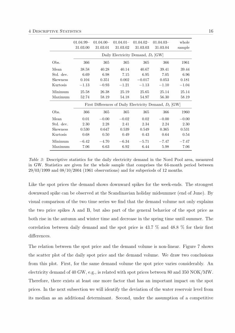
Table 3: Descriptive statistics for the daily electricity demand in the Nord Pool area, measuredin GW. Statistics are given for the whole sample that comprises the 64-month period between29/03/1999 and 08/10/2004 (1961 observations) and for subperiods of 12 months.
Like the spot prices the demand shows downward spikes for the week-ends. The strongest
downward spike can be observed at the Scandinavian holiday midsummer (end of June). By
visual comparison of the two time series we find that the demand volume not only explains
the two price spikes A and B, but also part of the general behavior of the spot price as
both rise in the autumn and winter time and decrease in the spring time until summer. The
correlation between daily demand and the spot price is 43.7 % and 48.8 % for their first
differences.
The relation between the spot price and the demand volume is non-linear. Figure 7 shows
the scatter plot of the daily spot price and the demand volume. We draw two conclusions
from this plot. First, for the same demand volume the spot price varies considerably. An
electricity demand of 40 GW, e.g., is related with spot prices between 80 and 350 NOK/MW.
Therefore, there exists at least one more factor that has an important impact on the spot
prices. In the next subsection we will identify the deviation of the water reservoir level from
its median as an additional determinant. Second, under the assumption of a competitive

4 Descriptive Statistics 17
market among producers the spot price equals the marginal cost of the last produced unit of
electricity. Given this assumption, Figure 7 indicates qualitatively that the marginal costs
are slightly, progressively increasing in the daily production volume.
There are at least three possible reasons why the spot prices could deviate from the unob-
servable marginal cost function:
1. The system prices at Nord Pool are usually determined one day, sometimes several
days before delivery. Therefore, the two quantities are determined asynchronously.
2. By using daily data we average across 24 hourly data of demand volumes and spot
prices, i. e. points of the marginal cost function. As the marginal cost function is
presumably convex, the average spot price is an upward biased estimator of the spot
price for the average demand volume. The absolute amount of this bias depends on
the production level.
3. The marginal cost function may vary over time. Apart from temporary plant outages
and from building new or breaking down old power plants, the level of the water
reservoirs and thus the production capacity of hydro plants has a major impact.
In our analysis we will not model the first two of the above mentioned effects, but take into
account the third one as we consider it to be the most crucial one.
4.4 Water Reservoir
The water reservoir level for Norway, Sweden, and Finland is published once a week in
percentage points of the total reservoir capacity in the Nord Pool area. Figure 8 in the
Appendix shows the time series of percentage levels and the deviation from its median
in percentage points of the total reservoir capacity. Table 4 presents the the key sample
statistics of the deviation. Note that the seasonal pattern in the level series is caused by
the melting period starting in April and the freezing period starting around November. The
first one increases the inflow into the water reservoirs while in the freezing period the inflows
are reduced. The seasonal component of the production volumes, i. e. the water outflow, has
only a minor impact on the reservoir level.

5 Estimation Procedure 18
01.04.99– 01.04.00– 01.04.01– 01.04.02– 01.04.03– whole31.03.00 31.03.01 31.03.02 31.03.03 31.03.04 sample
Obs. 52 52 52 52 53 282
Mean 3.82 4.96 −0.69 −8.38 −14.54 −3.66Std. dev. 3.75 2.52 5.92 9.48 3.72 9.39Skewness −0.190 0.483 −0.325 0.007 −0.393 −0.397Kurtosis −1.51 −0.12 −1.28 −1.58 −0.95 −1.24
Minimum −2.11 0.20 −11.63 −21.99 −22.05 −22.05Maximum 9.17 10.94 6.79 5.94 −9.61 10.94
Table 4: Descriptive statistics of the weekly water reservoir deviation from its median in the NordPool area, measured in percentage-points of the total reservoir capacity. Statistics are given forthe whole sample that comprises the 64-months period between 04/01/1999 and 08/10/2004 (280weekly observations) and for subperiods of 12 months.
Market participants know and anticipate the seasonal fluctuation of the reservoir level.
Therefore, as the scatter plot in Figure 9 shows, the absolute reservoir level contributes
only little to the explanation of spot prices. The correlation between the first differences of
the spot price and the reservoir level is only −3.7%.
The picture changes strongly if we replace the absolute reservoir level by its weekly deviation
in percentage-points from the observed reservoir level and its long-term median. We choose
the median instead of the mean because this value is published by Nord Pool and serves as a
reference for all market participants. Figure 10 shows a clear negative relation between the
reservoir deviation and the spot prices. The reason for this relationship is fairly obvious. If
a relatively high electricity demand coincides with below median water reservoir levels, this
demand has partly to be served by expensive plants like gas-fired turbines, i. e. the marginal
costs and, therefore, the spot prices are large. Vice versa, if there is an unexpected reservoir
surplus, a larger proportion of demand can be served by the cheap hydro plants.
5 Estimation Procedure
The basic structure of our estimation procedure is described in Figure 3. The total test
period runs from 05/24/2000 to 08/04/2004, i. e. 220 Wednesdays. We observe futures
prices on 216 of these Wednesdays, four of them are holidays. We take futures prices from
the following Thursday if that is not a holiday. Otherwise we skipped a week. This leaves

5 Estimation Procedure 19
n+1Tuesday Wednesday ((n+1)−th valuation day)
+ 1 week
11/01/1996 (Start of spot price series)
nTuesday Wednesday (n−th valuation day)
Estimation Period: Forecast of the deterministic component of spot pricesand of the demand on a weekly basis
03/29/1999 (Start of demand volume series)
Estimation of deterministic components
on a daily basisof spot prices and demand volumes
Aggregation into weekly data
Estimation of autoregressive deviations
Figure 3: This figure shows the moving time windows for estimating the deterministic and thestochastic part of the spot prices and for valuation of futures prices. We evaluate futures prices on220 Wednesdays, i. e. n = 1, . . . , 220, whereof we skip three that were holidays. The first valuationday is Wednesday, 05/24/2000, the last one is Wednesday, 08/04/2004.
us with 217 observations. For each of these valuation days we determine theoretical futures
prices using data up to the preceding Tuesday. These theoretical futures prices are compared
with observed prices.
We choose Wednesdays as valuation dates for two reasons: First, Wednesdays provide us
with the largest sample of trading days as very few holidays happen to be on Wednesdays.
Second, the weekly reservoir data are published on Wednesdays at 1 p. m. These data refer
to the reservoir level of the preceding Monday. Therefore, futures prices of Wednesdays are
the earliest ones that incorporate the new information on the water reservoir level.
For each of the 217 valuation days we perform the following estimation steps. First, we
estimate the deterministic component of the spot price in the reduced-form model, f(t),
and of the end-user demand in the equilibrium model, D(t), using daily data. This data
frequency is used to capture as much information as possible. We apply dummy variables for
day-of-week and holiday effects and a continuous, piecewise linear function to represent the
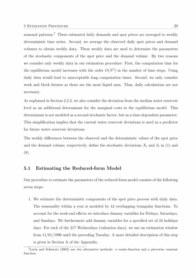
5 Estimation Procedure 20
seasonal patterns.7 These estimated daily demands and spot prices are averaged to weekly
deterministic time series. Second, we average the observed daily spot prices and demand
volumes to obtain weekly data. These weekly data are used to determine the parameters
of the stochastic components of the spot price and the demand volume. By two reasons
we consider only weekly data in our estimation procedure: First, the computation time for
the equilibrium model increases with the order O(N2) in the number of time steps. Using
daily data would lead to unacceptable long computation times. Second, we only consider
week and block futures as those are the most liquid ones. Thus, daily calculations are not
necessary.
As explained in Section 2.2.2, we also consider the deviation from the median water reservoir
level as an additional determinant for the marginal costs in the equilibrium model. This
determinant is not modeled as a second stochastic factor, but as a time-dependent parameter.
This simplification implies that the current water reservoir deviations is used as a predictor
for future water reservoir deviations.
The weekly differences between the observed and the deterministic values of the spot price
and the demand volume, respectively, define the stochastic deviations Xt and St in (1) and
(8).
5.1 Estimating the Reduced-form Model
Our procedure to estimate the parameters of the reduced-form model consists of the following
seven steps:
1. We estimate the deterministic components of the spot price process with daily data.
The seasonality within a year is modeled by 12 overlapping triangular functions. To
account for the week-end effects we introduce dummy variables for Fridays, Saturdays,
and Sundays. We furthermore add dummy variables for a specified set of 24 holidays
days. For each of the 217 Wednesdays (valuation days), we use an estimation window
from 11/01/1996 until the preceding Tuesday. A more detailed description of this step
is given in Section A of the Appendix.
7Lucia and Schwartz (2002) use two alternative methods: a cosine-function and a piecewise constantfunction.

5 Estimation Procedure 21
2. Based on the 217 regression results of Step 1 we calculate time series of deterministic
spot prices, f(T ), for the future maturity dates T of futures contracts up to 08/04/2005.
3. We aggregate the forecasted deterministic spot prices as well as the observed spot
prices to obtain weekly mean prices. The difference of these prices yields the weekly
time series of the spot price deviation, Xt.
4. We model the time series Xt as a first order autoregressive process
Xt = φXt−1 + εXt (11)
and use the estimate φ as a proxy for the speed of adjustment, κ = 1 − φ, and the
standard deviation of the regression as a proxy for σX .
5. Finally we calculate theoretical prices for week futures. If the agents are assumed to be
risk-neutral, the futures prices are obtained from (2) by setting λ to zero. Otherwise,
λ is obtained implicitly as described in Section 5.3. The prices of block futures are
computed as the average of the prices of the underlying week futures.
Our estimation design differs in two aspects from the estimation design by Lucia and
Schwartz (2002): First, we use a different approach for extracting the deterministic compo-
nents. Second, we aggregate daily data into weekly data.
5.2 Estimating the Equilibrium Model
We analyze the equilibrium by the following seven steps:
1. The seasonal component of the daily end-user demand in the Nord Pool area is esti-
mated analogously to the seasonal component of the spot price in the reduced-form
model. The estimation window begins on 03/29/1999 because Nord Pool does not
provide a longer times series for demand or production data. The estimation window
ends at the Tuesday of each particular valuation week.
2. We sum up the estimated daily seasonal volumes to obtain weekly seasonal demand
data. Analogously, we obtain the observed demand volumes per week. The differences

5 Estimation Procedure 22
between these two time series provides us with the stochastic component St on a weekly
basis.
3. We estimate the parameters ρ and σS of the AR(1)-process St as defined in (8).
4. For the estimation of the marginal cost function C ′t(D
∗t ) we simultaneously estimate
the slope coefficient c1 and the shift variable γ of the water reservoir deviation. Taking
the logarithm on (10) leads to the linear estimation equation
ln(Pt) = c0 + c1Dt + γWRDt + εct (12)
where autocorrelation is considered in εct .
5. We receive the cost function by integrating over the marginal cost function. We cannot
observe the fixed costs of production, however, as those are independent from the
demand, they are not needed for evaluating the risk premia.
6. The last necessary parameters are the tariff rate p that retailers charge their customers
and the interest rate. We linearly interpolate between the quarterly published tariff
data in order to achieve a weekly time series. The calculated weekly tariff prices vary
between 130 and 227 NOK/MW. For the interest rate we use daily observations.
7. Finally, we calculate theoretical prices for week futures. Under risk neutrality (ξ = 0)
they are easily obtained from (6). If agents are not risk-neutral, ξ is determined im-
plicitly as described in the next section. The theoretical futures prices are determined
recursively by dynamic programming.
5.3 Evaluation of Futures Prices
Our valuation analysis consists of three steps: First, we evaluate both models out-of-sample
as if market participants were risk-neutral, i. e. we assume λ = 0 for the reduced-form model
and ξ = 0 for the equilibrium model.
In the second step, we introduce risk aversion. For both models we estimate the implicit risk
aversion parameters by minimizing the root mean squared error (RMSE) between the ob-
served and the model prices by using observed futures prices of four subsequent Wednesdays.
6 Results 23
Average Results Full Sample
Mean Std. dev. Minimum Maximum
Reduced-form Model
Estimation window 11/01/1996 – 08/03/2004Observations 217 estimations 2833 daily obs.R2 0.917 0.041 0.848 0.965 0.965S. E. 16.23 2.30 11.12 18.03 17.02
Equilibrium Model
Estimation window 03/29/1999 – 08/03/2004Observations 217 estimations 1952 daily obs.R2 0.986 0.001 0.984 0.987 0.986S. E. 0.800 0.027 0.720 0.837 0.810
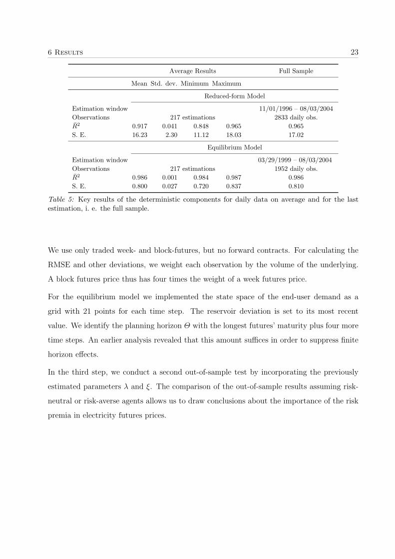
Table 5: Key results of the deterministic components for daily data on average and for the lastestimation, i. e. the full sample.
We use only traded week- and block-futures, but no forward contracts. For calculating the
RMSE and other deviations, we weight each observation by the volume of the underlying.
A block futures price thus has four times the weight of a week futures price.
For the equilibrium model we implemented the state space of the end-user demand as a
grid with 21 points for each time step. The reservoir deviation is set to its most recent
value. We identify the planning horizon Θ with the longest futures’ maturity plus four more
time steps. An earlier analysis revealed that this amount suffices in order to suppress finite
horizon effects.
In the third step, we conduct a second out-of-sample test by incorporating the previously
estimated parameters λ and ξ. The comparison of the out-of-sample results assuming risk-
neutral or risk-averse agents allows us to draw conclusions about the importance of the risk
premia in electricity futures prices.

6 Results 24
6 Results
6.1 Deterministic Components
In Table 5 we present some basic regression results for the deterministic components of the
demand and the spot prices. Detailed results for the full observation period are given in
Table 12 in the Appendix. We find that the holiday effects are more pronounced in the
demand volume than in the spot price. 22 out of 24 holidays have a significant effect on the
demand on the 1%-level. On the 5%-level, all 24 days significantly effect the demand and
only 14 holidays effect the spot price. Furthermore, all coefficients of the triangular basis
functions are significantly different from zero for the demand, but only four are significant for
the spot price on the 5%-level. The dummy variables for Fridays, Saturdays, and Sundays
are all highly significant for the spot price as well as for the demand volume.
Table 5 shows that the R2 is higher for the demand volume than for the spot price. The
standard error of the regression, standardized on the mean of spot prices or daily demand,
respectively, is larger for the spot price than for the demand. These results reflect the
intuition from Figures 5 and 6 that the seasonal patterns are much stronger in the demand
series than in the spot price series.
Figures 11 and 12 in the Appendix exemplarily plot the deterministic components of both
models for the estimation period. Visual inspection affirms that the deterministic compo-
nent of the demand explains total demand much better than in the case of the spot price.
The residuals of the spot price may even exceed the deterministic component. The regular
downward spikes in the deterministic components as well as in the observed data are due
to the end-of-week effects. We like to point out that the use of monthly dummy variables
instead of triangular functions would result in a rather irregular behavior of the stochastic
component for both exogenous variables.
6.2 Stochastic Processes
As described in Section 5 we estimate the AR(1)-processes of the residuals Xt and St, re-
spectively, from weekly data by non-linear least squares. The upper part of Table 6 shows
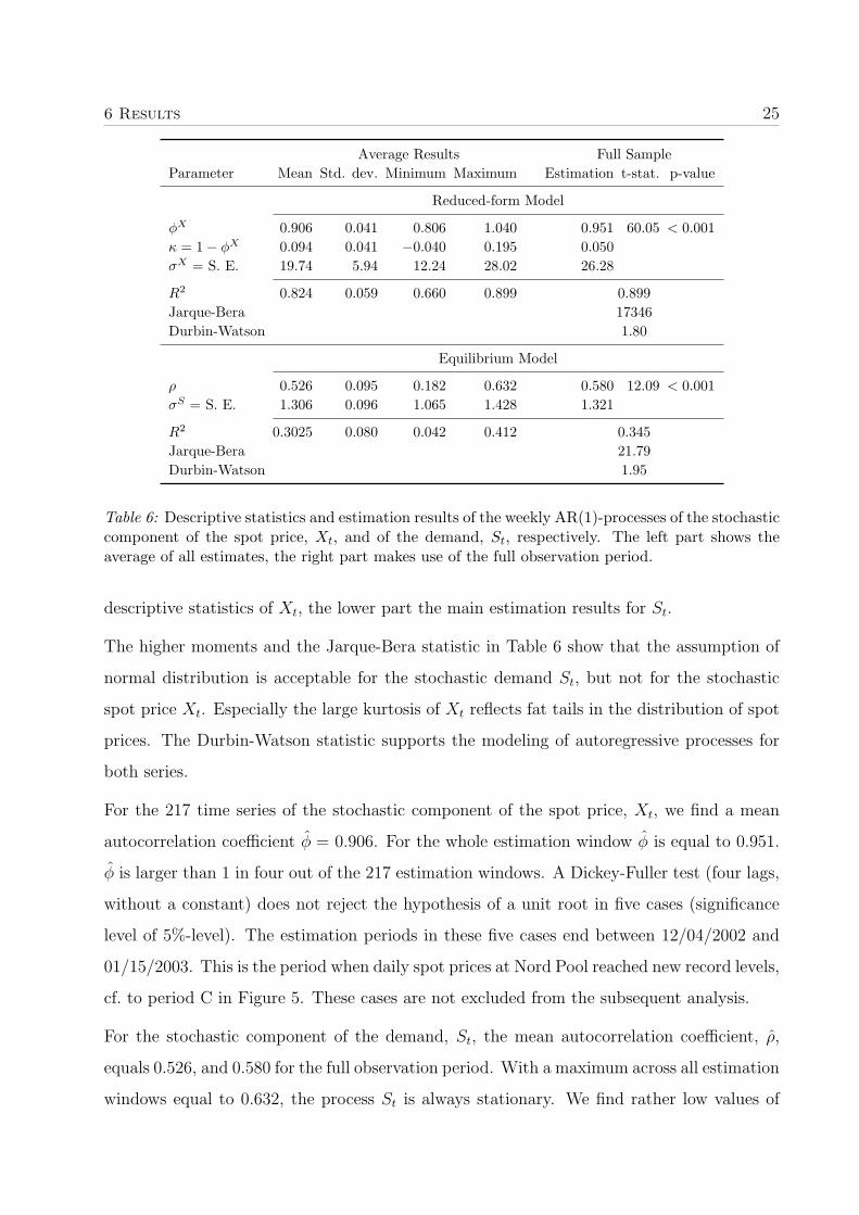
6 Results 25
Average Results Full SampleParameter Mean Std. dev. Minimum Maximum Estimation t-stat. p-value
Reduced-form Model
φX 0.906 0.041 0.806 1.040 0.951 60.05 < 0.001κ = 1− φX 0.094 0.041 −0.040 0.195 0.050σX = S. E. 19.74 5.94 12.24 28.02 26.28
R2 0.824 0.059 0.660 0.899 0.899Jarque-Bera 17346Durbin-Watson 1.80
Equilibrium Model
ρ 0.526 0.095 0.182 0.632 0.580 12.09 < 0.001σS = S. E. 1.306 0.096 1.065 1.428 1.321
R2 0.3025 0.080 0.042 0.412 0.345Jarque-Bera 21.79Durbin-Watson 1.95
Table 6: Descriptive statistics and estimation results of the weekly AR(1)-processes of the stochasticcomponent of the spot price, Xt, and of the demand, St, respectively. The left part shows theaverage of all estimates, the right part makes use of the full observation period.
descriptive statistics of Xt, the lower part the main estimation results for St.
The higher moments and the Jarque-Bera statistic in Table 6 show that the assumption of
normal distribution is acceptable for the stochastic demand St, but not for the stochastic
spot price Xt. Especially the large kurtosis of Xt reflects fat tails in the distribution of spot
prices. The Durbin-Watson statistic supports the modeling of autoregressive processes for
both series.
For the 217 time series of the stochastic component of the spot price, Xt, we find a mean
autocorrelation coefficient φ = 0.906. For the whole estimation window φ is equal to 0.951.
φ is larger than 1 in four out of the 217 estimation windows. A Dickey-Fuller test (four lags,
without a constant) does not reject the hypothesis of a unit root in five cases (significance
level of 5%-level). The estimation periods in these five cases end between 12/04/2002 and
01/15/2003. This is the period when daily spot prices at Nord Pool reached new record levels,
cf. to period C in Figure 5. These cases are not excluded from the subsequent analysis.
For the stochastic component of the demand, St, the mean autocorrelation coefficient, ρ,
equals 0.526, and 0.580 for the full observation period. With a maximum across all estimation
windows equal to 0.632, the process St is always stationary. We find rather low values of
6 Results 26
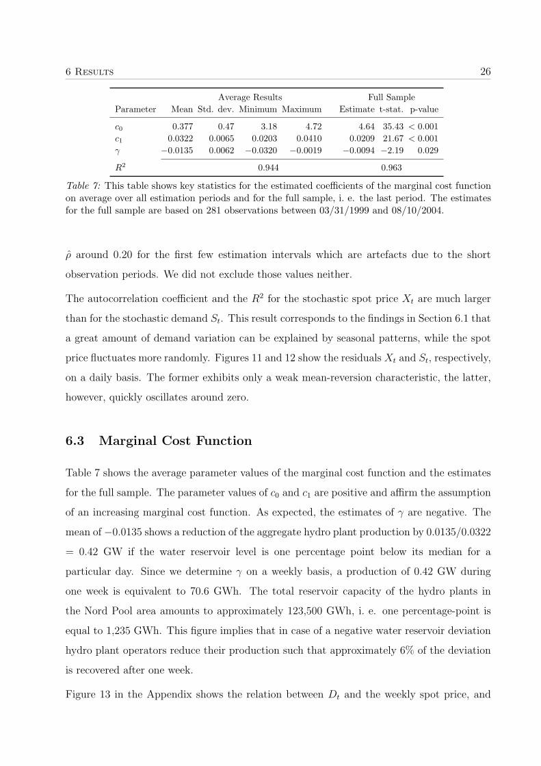
Average Results Full SampleParameter Mean Std. dev. Minimum Maximum Estimate t-stat. p-value
c0 0.377 0.47 3.18 4.72 4.64 35.43 < 0.001c1 0.0322 0.0065 0.0203 0.0410 0.0209 21.67 < 0.001γ −0.0135 0.0062 −0.0320 −0.0019 −0.0094 −2.19 0.029
R2 0.944 0.963
Table 7: This table shows key statistics for the estimated coefficients of the marginal cost functionon average over all estimation periods and for the full sample, i. e. the last period. The estimatesfor the full sample are based on 281 observations between 03/31/1999 and 08/10/2004.
ρ around 0.20 for the first few estimation intervals which are artefacts due to the short
observation periods. We did not exclude those values neither.
The autocorrelation coefficient and the R2 for the stochastic spot price Xt are much larger
than for the stochastic demand St. This result corresponds to the findings in Section 6.1 that
a great amount of demand variation can be explained by seasonal patterns, while the spot
price fluctuates more randomly. Figures 11 and 12 show the residuals Xt and St, respectively,
on a daily basis. The former exhibits only a weak mean-reversion characteristic, the latter,
however, quickly oscillates around zero.
6.3 Marginal Cost Function
Table 7 shows the average parameter values of the marginal cost function and the estimates
for the full sample. The parameter values of c0 and c1 are positive and affirm the assumption
of an increasing marginal cost function. As expected, the estimates of γ are negative. The
mean of −0.0135 shows a reduction of the aggregate hydro plant production by 0.0135/0.0322
= 0.42 GW if the water reservoir level is one percentage point below its median for a
particular day. Since we determine γ on a weekly basis, a production of 0.42 GW during
one week is equivalent to 70.6 GWh. The total reservoir capacity of the hydro plants in
the Nord Pool area amounts to approximately 123,500 GWh, i. e. one percentage-point is
equal to 1,235 GWh. This figure implies that in case of a negative water reservoir deviation
hydro plant operators reduce their production such that approximately 6% of the deviation
is recovered after one week.
Figure 13 in the Appendix shows the relation between Dt and the weekly spot price, and
6 Results 27
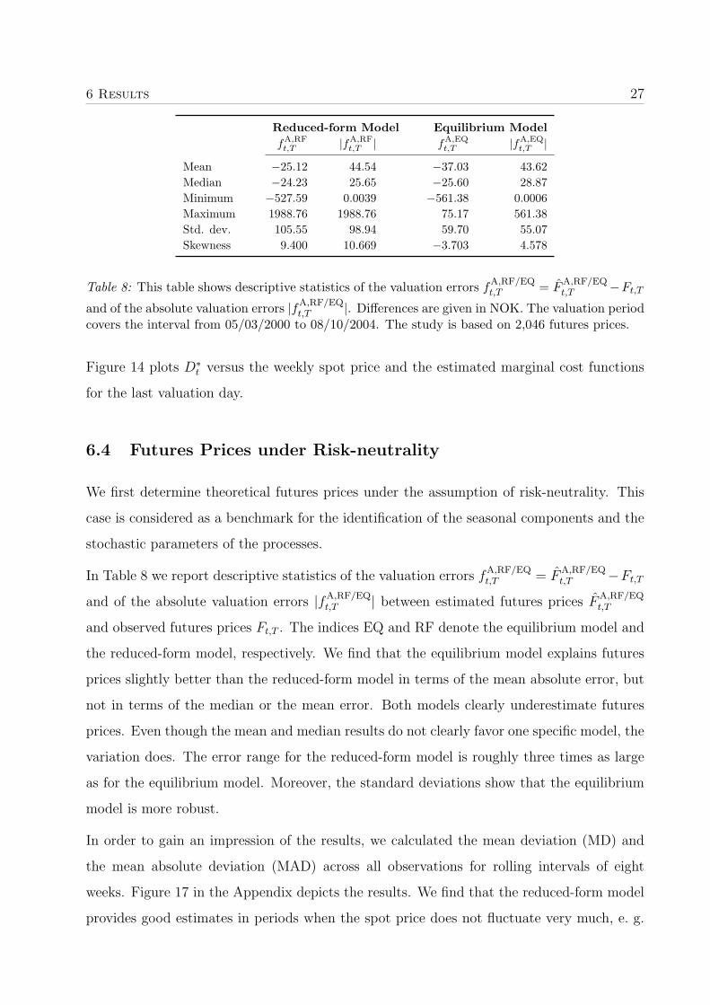
Reduced-form Model Equilibrium ModelfA,RF
t,T |fA,RFt,T | fA,EQ
t,T |fA,EQt,T |
Mean −25.12 44.54 −37.03 43.62Median −24.23 25.65 −25.60 28.87Minimum −527.59 0.0039 −561.38 0.0006Maximum 1988.76 1988.76 75.17 561.38Std. dev. 105.55 98.94 59.70 55.07Skewness 9.400 10.669 −3.703 4.578
Table 8: This table shows descriptive statistics of the valuation errors fA,RF/EQt,T = F
A,RF/EQt,T −Ft,T
and of the absolute valuation errors |fA,RF/EQt,T |. Differences are given in NOK. The valuation period
covers the interval from 05/03/2000 to 08/10/2004. The study is based on 2,046 futures prices.
Figure 14 plots D∗t versus the weekly spot price and the estimated marginal cost functions
for the last valuation day.
6.4 Futures Prices under Risk-neutrality
We first determine theoretical futures prices under the assumption of risk-neutrality. This
case is considered as a benchmark for the identification of the seasonal components and the
stochastic parameters of the processes.
In Table 8 we report descriptive statistics of the valuation errors fA,RF/EQt,T = F
A,RF/EQt,T −Ft,T
and of the absolute valuation errors |fA,RF/EQt,T | between estimated futures prices F
A,RF/EQt,T
and observed futures prices Ft,T . The indices EQ and RF denote the equilibrium model and
the reduced-form model, respectively. We find that the equilibrium model explains futures
prices slightly better than the reduced-form model in terms of the mean absolute error, but
not in terms of the median or the mean error. Both models clearly underestimate futures
prices. Even though the mean and median results do not clearly favor one specific model, the
variation does. The error range for the reduced-form model is roughly three times as large
as for the equilibrium model. Moreover, the standard deviations show that the equilibrium
model is more robust.
In order to gain an impression of the results, we calculated the mean deviation (MD) and
the mean absolute deviation (MAD) across all observations for rolling intervals of eight
weeks. Figure 17 in the Appendix depicts the results. We find that the reduced-form model
provides good estimates in periods when the spot price does not fluctuate very much, e. g.

6 Results 28
during summer 2000. Contrary, the equilibrium model provides better results when the
spot price exhibits its characteristic spikes. For example, the extreme weather conditions
in combination with a very low reservoir level in winter 2002/03 result in extremely high
prices. During this period the equilibrium model explains futures prices considerably better
than the reduced-form model.
We argue that there are two main reasons for the better performance of the production-based
equilibrium approach during volatile markets: First, the reduced-form model cannot reflect
the distribution of the spot price deviations Xt. As shown in Table 6, the Jarque-Bera statis-
tic indicates that residuals from the AR(1)-estimation of the stochastic spot price are not
normally distributed. The production-based approach in the equilibrium model introduces
the skewness of spot prices by transforming normally distributed demand deviations, St, into
right-skewed spot prices due to the increasing marginal cost function.
Second, the stochastic deviation of the spot price, Xt, represents a larger part of spot and
futures prices in the reduced-form model, cf. Figure 11. A large value of Xt can be due to
an extreme event (e. g., a week of cold weather) that does not affect futures prices or it can
be caused by lasting changes in the determinants of electricity prices (e. g., a change in the
water reservoir deviation) that does affect futures prices. The former case would require a
small value of κ, the latter a large value of κ. The estimated κ is supposed to be somewhere
in between.
For the stochastic part of the demand the described problem is of less importance: First,
changes in the stochastic demand residual, St, are mostly caused by weather conditions
and, thus, will in general fade out quickly. This is reflected by the low value of ρ, cf.
Table 6. Second, the deterministic component of the demand provides good estimates of
future demand in comparison to the deterministic component of the spot price, cf. Figure
12. Therefore, St has a smaller impact on forecasted demands and marginal costs than Xt.
We conclude that a large absolute value of Xt may lead to large deviations between the
theoretical and the observed futures prices.
Figure 17 shows that the value of the mean meviation is mostly negative for both models,
restating that both models tend to underestimate the observed futures prices. For the time
period between Dec. 2002 and Jan. 2003, however, futures prices are strongly overestimated
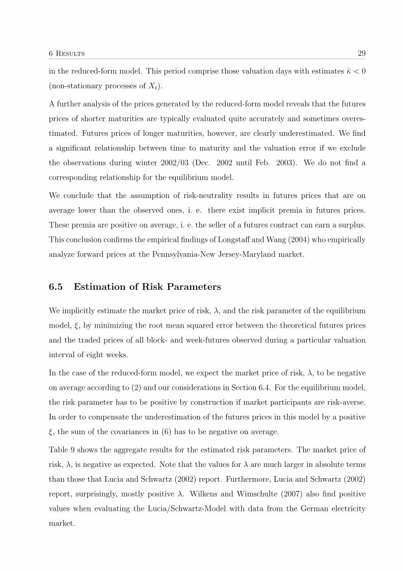
6 Results 29
in the reduced-form model. This period comprise those valuation days with estimates κ < 0
(non-stationary processes of Xt).
A further analysis of the prices generated by the reduced-form model reveals that the futures
prices of shorter maturities are typically evaluated quite accurately and sometimes overes-
timated. Futures prices of longer maturities, however, are clearly underestimated. We find
a significant relationship between time to maturity and the valuation error if we exclude
the observations during winter 2002/03 (Dec. 2002 until Feb. 2003). We do not find a
corresponding relationship for the equilibrium model.
We conclude that the assumption of risk-neutrality results in futures prices that are on
average lower than the observed ones, i. e. there exist implicit premia in futures prices.
These premia are positive on average, i. e. the seller of a futures contract can earn a surplus.
This conclusion confirms the empirical findings of Longstaff and Wang (2004) who empirically
analyze forward prices at the Pennsylvania-New Jersey-Maryland market.
6.5 Estimation of Risk Parameters
We implicitly estimate the market price of risk, λ, and the risk parameter of the equilibrium
model, ξ, by minimizing the root mean squared error between the theoretical futures prices
and the traded prices of all block- and week-futures observed during a particular valuation
interval of eight weeks.
In the case of the reduced-form model, we expect the market price of risk, λ, to be negative
on average according to (2) and our considerations in Section 6.4. For the equilibrium model,
the risk parameter has to be positive by construction if market participants are risk-averse.
In order to compensate the underestimation of the futures prices in this model by a positive
ξ, the sum of the covariances in (6) has to be negative on average.
Table 9 shows the aggregate results for the estimated risk parameters. The market price of
risk, λ, is negative as expected. Note that the values for λ are much larger in absolute terms
than those that Lucia and Schwartz (2002) report. Furthermore, Lucia and Schwartz (2002)
report, surprisingly, mostly positive λ. Wilkens and Wimschulte (2007) also find positive
values when evaluating the Lucia/Schwartz-Model with data from the German electricity
market.

6 Results 30
Reduced-form Model Equilibrium Modelλ ξ
Mean −0.2389 0.1569Median −0.2632 0.0270Minimum −0.7998 −0.6566Maximum 1.0204 1.9497Std. dev. 0.3175 0.4092
Table 9: This table shows the results of the implicitly estimated parameters of risk aversion.
The larger absolute values of λ in our study are due to our approach of estimating the
autocorrelation on a weekly basis. Recall that the risk premium in the reduced-form model
is equal to −λσX
κ(1− e−κ(T−t)). In order to achieve a certain risk premium, λ must increase
if the fraction σX
κdecreases, c. p. From our weekly approach we receive larger estimates for
the speed of adjustment, κ, and for the spot price volatility, σX , than Lucia and Schwartz
(2002) do. Our estimates for κ are on average around 0.09 per week, and for σX around 20
NOK per week (cf. Table 6), i. e. σX
κ= 222. Lucia and Schwartz (2002) report a κ of 0.01 per
day, and a value of 9 for σX , i. e. σX
κ= 900. This larger value results from not considering
autocorrelation of higher lags in the daily residuals, leading to an overestimation of σX .
The different test periods also account for part of the difference in absolute values and
especially for negative instead of positive values of λ. Lucia and Schwartz (2002) test their
model during a twelve-month period in 1998/1999 when spot prices were lower on average
than in the years before. Therefore, their estimated deterministic component f(t) of the
spot price overestimates the spot prices in the test period, leading to mostly positive values
of λ. We encountered the opposite situation. Table 1 shows that the twelve-month average
spot price increased until 2003 and stayed on a high level until the end of our available
time series. From an ex-post perspective, the deterministic component of the spot price
then inevitably underestimates the observed and future spot prices. If market participants
can partly predict such increasing spot prices – e. g. by considering water reservoir levels –
and evaluate futures accordingly, the reduced-form model must underestimate futures prices
when risk-neutrality is assumed. A negative λ that is appropriately large in absolute terms
can compensate such estimation errors.
As an exception in our sample, λ adopts large positive values in the intervals covering
December 2002 and January 2003 when spot prices were extremely high. This effect is
6 Results 31
caused by negative estimates of κ in those particular intervals.
Depending on the sign of λ, the term −λσX
κ(1 − e−κ(T−t))) is either strictly positive or
strictly negative for all maturities, it increases and asymptotically converges to a constant
with increasing time to maturity (T − t). Thus, it matches the curve of valuation errors that
basically increases with time-to-maturity as described in the previous section. Figure 18 in
the Appendix shows a scatter plot of the in-sample estimated risk premia in the reduced-
form model. In the majority of observations, those are clearly positive and adopt values up
to 180 NOK. Especially during the winter 2002/03, the risk premia reach enormous negative
values that do not seem economically meaningful.
The time series of λ features a level-autocorrelation of 0.98. We therefore conclude that λ
contains valuable information and contributes to forecasting futures prices even when applied
out-of-sample as we test in the next section even though we observe eight changes of sign
in the time series. The means between λ in warm and cold periods (April until September
vs. October until March) show little difference. We conclude that λ does not incorporate
seasonal effects that discriminate between summer and winter.
The estimated values of ξ in the equilibrium model are mostly and on average positive as
expected. However, in 36 out of 217 cases ξ is negative. The negative values mostly occur
in subsequent valuation intervals. The level-autocorrelation of ξ amounts to 0.95, i. e. ξ is
supposed to improve futures pricing out-of-sample, too. However, the time series of ξ exhibits
six changes of sign. For those valuation dates we expect the results from the out-of-sample
test in Section 6.6 to be worse than those from the risk-neutral evaluation.
The technical reason for negative ξ lies in the covariance term of (6). In the majority of
cases, the expected future spot price is smaller than the observed futures price as shown in
the previous section. In order to generate a positive risk premium with a positive value of ξ,
the sum of covariances in (6) must be negative. To meet this requirement, the covariances
between the future demands Dt times the end-user price and the next period’s futures price
have to be smaller than the covariances between the future production costs C(Dt) and the
futures price.
For low demand volumes the slope of the cost function (i. e. the marginal cost function)
is smaller than the average end-user price. These low demand volumes would therefore
6 Results 32
contribute positively to the covariance term. If the probability of high demand volumes is
small, the whole covariance term can be positive.
According to the reasoning above, negative values of ξ should be possible when only futures
maturing in the summer time are evaluated, but not necessarily when the valuation day lies
in the summer time as it is the case in our results.
However, the estimation of the marginal cost function used at those particular valuation dates
is dominated by observations at summer dates. This effect arises from the beginning of each
estimation period at the end of March 1999. Therefore, each estimation of the marginal cost
function is based on more summer than winter observations. This effect especially holds
for the earlier valuation dates. Furthermore, the estimation of the marginal cost functions
before winter 2002/03 in general lacks observations of extremely large spot prices. Both facts
lead to estimates of the marginal cost function with a slope that is too low.
Our analysis of the risk premia at these particular days has shown that the underestimated
marginal cost function forces the parameter ξ to be negative in such cases. Still, for higher
production levels or low reservoir levels, the cost function is steep enough to support positive
values of ξ.
Generally, in the equilibrium model a non-zero value of ξ does not shift the whole futures
curve into one direction as the reduced-form model does, but adds large premia for short
maturities and lower premia for long maturities. Also a combination of positive premia
at the short end and negative premia for longer maturities may occur. Figure 19 in the
Appendix shows estimated risk premia along time to maturity. The risk premium in the
equilibrium model adopts its extreme values for some short maturity. It approaches zero
for long maturities and therefore cannot compensate theoretical miss-pricing of long-term
futures. It indirectly depends on seasonal effects as it considers covariances between futures
prices on the one hand side and production costs, marginal production costs, and demand
volumes on the other hand side.
Thus, if the calculation with ξ = 0 shows a large difference between calculated and observed
prices along the whole futures curve, even a large absolute value of ξ contributes only little
to the reduction of the estimation errors for long maturities. On the other hand side, if the
estimation of ξ is based on few futures contracts with only short maturities, i. e. after August
6 Results 33
Reduced-form Model Equilibrium ModelfC,RF
t,T |fC,RFt,T | fC,EQ
t,T |fC,EQt,T |
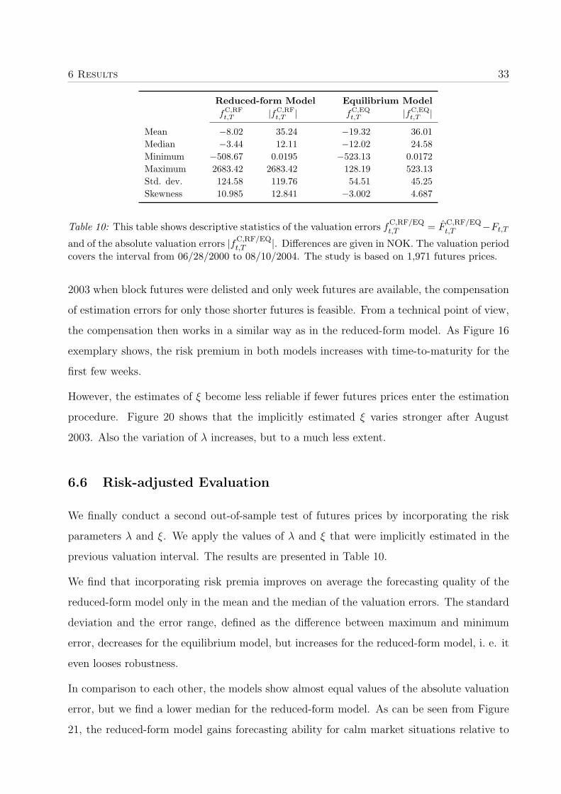
Mean −8.02 35.24 −19.32 36.01Median −3.44 12.11 −12.02 24.58Minimum −508.67 0.0195 −523.13 0.0172Maximum 2683.42 2683.42 128.19 523.13Std. dev. 124.58 119.76 54.51 45.25Skewness 10.985 12.841 −3.002 4.687
Table 10: This table shows descriptive statistics of the valuation errors fC,RF/EQt,T = F
C,RF/EQt,T −Ft,T
and of the absolute valuation errors |fC,RF/EQt,T |. Differences are given in NOK. The valuation period
covers the interval from 06/28/2000 to 08/10/2004. The study is based on 1,971 futures prices.
2003 when block futures were delisted and only week futures are available, the compensation
of estimation errors for only those shorter futures is feasible. From a technical point of view,
the compensation then works in a similar way as in the reduced-form model. As Figure 16
exemplary shows, the risk premium in both models increases with time-to-maturity for the
first few weeks.
However, the estimates of ξ become less reliable if fewer futures prices enter the estimation
procedure. Figure 20 shows that the implicitly estimated ξ varies stronger after August
2003. Also the variation of λ increases, but to a much less extent.
6.6 Risk-adjusted Evaluation
We finally conduct a second out-of-sample test of futures prices by incorporating the risk
parameters λ and ξ. We apply the values of λ and ξ that were implicitly estimated in the
previous valuation interval. The results are presented in Table 10.
We find that incorporating risk premia improves on average the forecasting quality of the
reduced-form model only in the mean and the median of the valuation errors. The standard
deviation and the error range, defined as the difference between maximum and minimum
error, decreases for the equilibrium model, but increases for the reduced-form model, i. e. it
even looses robustness.
In comparison to each other, the models show almost equal values of the absolute valuation
error, but we find a lower median for the reduced-form model. As can be seen from Figure
21, the reduced-form model gains forecasting ability for calm market situations relative to
6 Results 34
the equilibrium model, but fails during volatile periods. This leads to a more than twice
as high standard deviation of the errors of the reduced-form model than of the equilibrium
model. Specifically, this result is driven by some extreme forecasting errors that derive from
large prices in the winter 2002/03.
Both models continue to underestimate the futures prices on average, even though to a much
lesser extent. We conjectured in the previous sections that the different functional forms of
the risk premium term structures will allow the reduced-form model to better compensate
for mispricing of long-term futures. Therefore, we regress the valuation error on the time
to maturity. We do not find a significant relationship for the equilibrium model. However,
we find a significant positive relationship for the reduced-form model, i. e. the underpricing
decreases on average with increasing time to maturity.
We again examine the correlations between the error measures of both models. For the
valuation error we find a correlation of 26.6%, for the absolute valuation error it is 31.9%.
Both dropped slightly compared to our first study. This confirms that the adjustment by
incorporating risk premia works differently in both models.
As discussed the risk premia necessarily contain a fraction due to the misestimation of
expected futures prices and another one for actual, but unobservable risk premia. These
two cannot be separated. However, if we assume that the errors of the estimation of the
expected spot prices are symmetrically distributed with a constant – presumably negative
– mean, than the estimated risk premia should represent fraction of the actual risk premia
plus a constant.
In order to evaluate the estimated risk premia, ΛC, RF/EQt,T = F
C, RF/EQt,T −F
A, RF/EQt,T , we regress
them on the valuation errors fA,RF/EQt,T from our first study:
ΛC, RF/EQt,T = ζ
RF/EQ0 + ζ
RF/EQA f
A,RF/EQt,T + u
RF/EQt,T (13)
with uRF/EQt,T i. i. d. distributed. The results are given in table 11.
As expected, the estimated constants are positive, indicating that the risk premia cover up
part of the undervaluation. Surprisingly, the slope ζRFA for the reduced-form model does
not significantly differ from zero. Thus, on average the risk premium in the reduced-form
model does not capture any structure of the errors in our first study. However, we did the
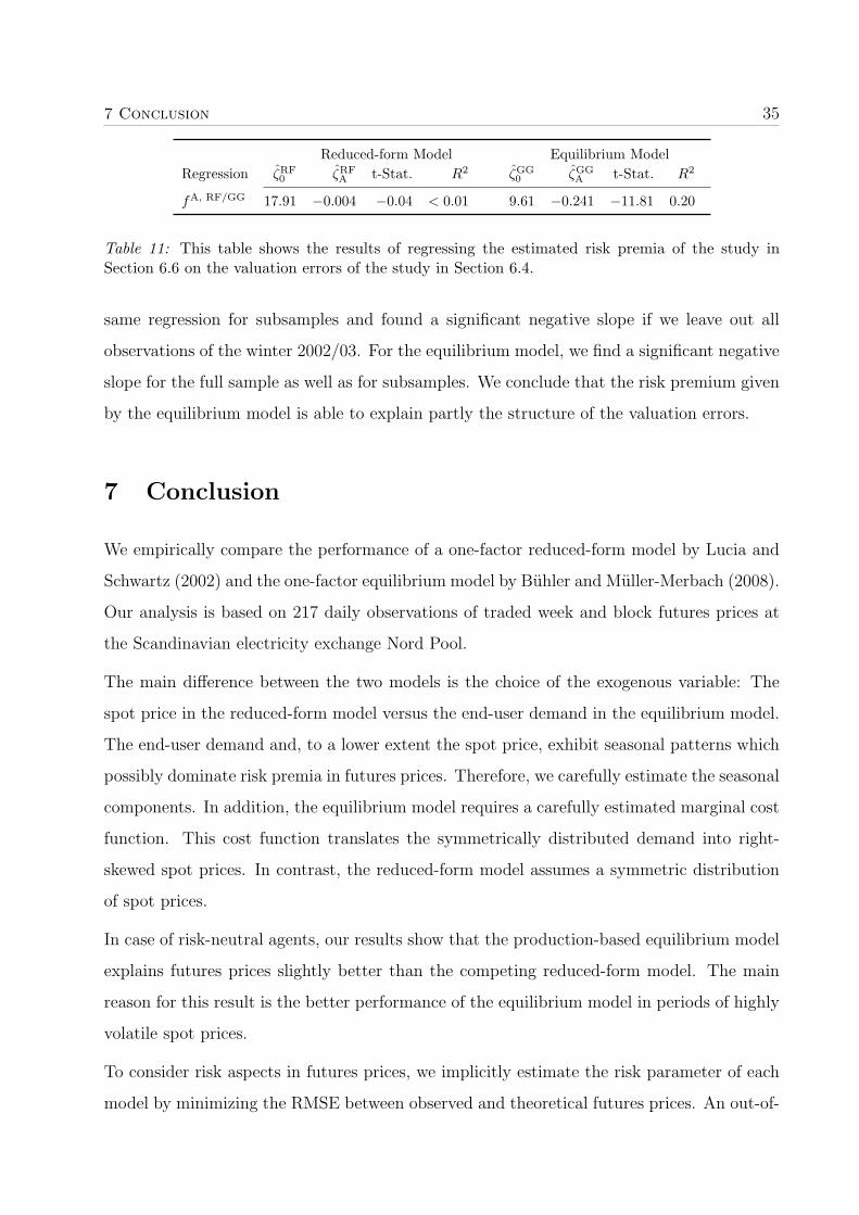
7 Conclusion 35
Reduced-form Model Equilibrium ModelRegression ζRF
0 ζRFA t-Stat. R2 ζGG
0 ζGGA t-Stat. R2
fA, RF/GG 17.91 −0.004 −0.04 < 0.01 9.61 −0.241 −11.81 0.20
Table 11: This table shows the results of regressing the estimated risk premia of the study inSection 6.6 on the valuation errors of the study in Section 6.4.
same regression for subsamples and found a significant negative slope if we leave out all
observations of the winter 2002/03. For the equilibrium model, we find a significant negative
slope for the full sample as well as for subsamples. We conclude that the risk premium given
by the equilibrium model is able to explain partly the structure of the valuation errors.
7 Conclusion
We empirically compare the performance of a one-factor reduced-form model by Lucia and
Schwartz (2002) and the one-factor equilibrium model by Buhler and Muller-Merbach (2008).
Our analysis is based on 217 daily observations of traded week and block futures prices at
the Scandinavian electricity exchange Nord Pool.
The main difference between the two models is the choice of the exogenous variable: The
spot price in the reduced-form model versus the end-user demand in the equilibrium model.
The end-user demand and, to a lower extent the spot price, exhibit seasonal patterns which
possibly dominate risk premia in futures prices. Therefore, we carefully estimate the seasonal
components. In addition, the equilibrium model requires a carefully estimated marginal cost
function. This cost function translates the symmetrically distributed demand into right-
skewed spot prices. In contrast, the reduced-form model assumes a symmetric distribution
of spot prices.
In case of risk-neutral agents, our results show that the production-based equilibrium model
explains futures prices slightly better than the competing reduced-form model. The main
reason for this result is the better performance of the equilibrium model in periods of highly
volatile spot prices.
To consider risk aspects in futures prices, we implicitly estimate the risk parameter of each
model by minimizing the RMSE between observed and theoretical futures prices. An out-of-

REFERENCES 36
sample test shows that both models result in lower average errors with a slight advantage for
the reduced-form model. However, the reduced-form model exhibits a much larger standard
deviation of the valuation errors, as it still fails to capture price spikes appropriately.
Finally, we compare the model-free estimates of risk premia in futures prices with the model
dependent premia. Our results support the term structure of risk premia as derived form
the equilibrium model. The reduced-form model has not enough flexibility to explain the
observed premia.
The implementation of the equilibrium model is much more challenging compared to the
reduced-from model. It requires more input data and considerably higher computational
effort. This advantage of the reduced-form model is diminished if the spot price is modeled
by jump-diffusions in order to cope with price peaks. Villaplana (2003) and Geman and
Roncoroni (2006) provide examples in this direction.
References
Audet, N., Heiskanen, P., Keppo, J., and Vehvilainen, I. (2002). Modelling of Electricity
Forward Curve Dynamics. Working Paper, University of Michigan, USA.
Basak, S. and Chabakauri, G. (2007). Dynamic Mean-Variance Asset Allocation. Working
Paper, London Business School.
Benth, F. E., Cartea, A., and Kiesel, R. (2007). Pricing Forward Contracts in Power Markets
by the Certainty Equivalence Principle: Explaining the Sign of the Risk Premium. Working
Paper.
Bessembinder, H. and Lemmon, M. (2002). Equilibrium Pricing and Optimal Hedging in
Electricity Forward Markets. Journal of Finance, 57(3), 1347–1382.
Buhler, W. and Muller-Merbach, J. (2008). Risk Premia of Electricity Futures: A Dynamic
Equilibrium Model. In Geman, H. (Ed.), Risk Management in Commodity Markets, chap-
ter 5, 61–80. Chichester: Wiley.
Bye, T. (2003). A Nordic Energy Market under Stress. Economic Survey, (4), 26–37.
REFERENCES 37
Cartea, A. and Figueroa, M. G. (2005). Pricing in Electricity Markets: A Mean Reverting
Jump Diffusion Model with Seasonality. Applied Mathematical Finance, 12(4), 313–335.
Geman, H. (2005). Commodities and Commodity Derivatives. Chichester: Wiley.
Geman, H. and Roncoroni, A. (2006). Understanding the Fine Structure of Electricity Prices.
Journal of Business, 79(3), 7–14.
Geman, H. and Vasicek, O. (2001). Plugging into Electricity. Risk, 93–97.
Koekebakker, S. and Ollmar, F. (2005). Forward Curve Dynamics in the Nordic Electricity
Market. Managerial Finance, 31(6), 73–94.
Longstaff, F. A. and Wang, A. W. (2004). Electricity Forward Prices: A High-frequency
Empirical Analysis. Journal of Finance, 59(4), 1877–1900.
Lucia, J. J. and Schwartz, E. S. (2002). Electricity Prices and Power Derivatives: Evidence
from the Nordic Power Exchange. Review of Derivatives Research, 5(1), 5–50.
Nord Pool ASA (ed.) (1998). Elbørsen – the nordic power exchange’s 5th anniversary issue.
Nord Pool ASA (ed.) (2004). Trading rules for financial electricity contracts and certificate
contracts. Manual.
Pilipovic, D. (1997). Energy Risk. New York et al.: McGraw-Hill.
Routledge, B. R., Seppi, D. J., and Spatt, C. S. (2001). The Spark Spread: Cross-Commodity
Equilibrium Restrictions and Electricity. Working Paper, Carnegie Mellon University.
Ullrich, C. J. (2007). Constrained Capacity and Equilibrium Forward Premia in Electricity
Markets. Working Paper, Pennsylvania State University.
Villaplana, P. (2003). Pricing Power Derivatives: A Two-factor Jump-diffusion Approach.
Working Paper.
Wilkens, S. and Wimschulte, J. (2007). The Pricing of Electricity Futures: Evidence from
the European Energy Exchange. The Journal of Futures Markets, 27(4), 387–410.

A Estimation of the Deterministic Components A.1
A Estimation of the Deterministic Components
To model the piecewise linear function of the seasonal pattern, we define 12 overlapping
triangular functions Mi,t around certain equidistant calendar days ti.
The selection of triangular functions Mi,t as regressors yields a piecewise linear and contin-
uous function for the seasonal component, cf. Figure 4. Note that this procedure does not
require more coefficients than conventional dummy variables.
The effects of specific days on the spot price or the daily demand are captured by dummy
variables FRIt, SATt, and SUNt for week-end days, and Hh,t for holidays and for additional
days with a significant impact on the endogenous variable. The residual in the regression is
assumed to follow an autoregressive process whose lag is determined by the Akaike criterion.
The triangular functions are defined as follows:
Mi,t =1
28·
∆t− (ti − t) , 0 ≤ ti − t < ∆t
∆t− (t− ti) , 0 < t− ti < ∆t
0 , elsewhere
(14)
with ∆t = 28 days and the following calendar days ti:
t1 01/01 t2 01/29 t3 02/26 t4 03/26 t5 04/23 t6 05/21
t7 06/18 t8 08/14 t9 09/11 t10 10/09 t11 11/06 t12 12/04
We use this procedure for both models. We choose 13 calendar days (instead of 12 corre-
sponding to the calendar months) for the simple reason that 365 mod 13 = 1, i. e. we can
cover one year more regularly when applying 13 instead of 12 intervals. July 16 and 17 are
used as benchmark days, i. e. not covered by any of the triangular functions. We choose
these days as they are the ones with the lowest production in the long-term average.
The regression equation for the reduced-form model is given by:
Pt = β0 +12∑i=1
βiMi,t + βFRIFRIt + βSATSATt + βSUNSUNt +∑
h
βhHh,t + εPt (15)
with εPt = φ1ε
Pt−1 + φ2ε
Pt−2 + φ3ε
Pt−3 + . . . + uP
t , uPt ∼ N (0, σP ) (16)

A Estimation of the Deterministic Components A.2
M1 M2 M 3 M4
β2
β4
β1
β3
M1β1M2β2
M 3β3
M4β4
M2β2 M4β4M1β1 M 3β3
1
28 56 84 112 days
+ + + + ...
Figure 4: This figure illustrates the principle of describing the deterministic components in thespot price and in the demand series.

A Estimation of the Deterministic Components A.3
The time index t in (15) and (16) runs from 11/01/1996 until the Tuesday preceding the
valuation day (Wednesday). For the equilibrium model the endogenous variable Pt in (15) is
replaced by the daily demand Dt and the autoregressive residuals have three lags only. The
estimation results for the total observation period of spot prices and daily demand volumes
are given in Table 12.
Spot Prices Electricity Demand(Reduced-form Model) (Equilibrium Model)
Estimation Window 11/01/1996–08/03/2004 03/29/1999–08/03/2004No. of obs. 2833 1955
Estimate [NOK] t-Statistic Estimate [GW] t-Statisticβ0 (Const.) 125.00 3.64 30.83 49.11β1 (01/01) 137.08 3.63 19.93 21.10β2 (01/29) 74.33 1.98 18.91 20.09β3 (02/26) 69.97 1.90 18.26 19.52β4 (03/26) 42.88 1.21 13.40 14.33β5 (04/23) 34.72 1.05 8.22 9.16β6 (05/21) 25.40 0.87 4.96 5.57β7 (06/18) 34.40 1.53 2.99 3.13β8 (08/14) 31.30 1.36 3.30 3.34β9 (09/11) 38.53 1.27 4.96 5.32β10 (10/09) 42.21 1.23 9.60 10.20β11 (11/06) 64.78 1.77 14.00 14.89β12 (12/04) 102.59 2.75 16.76 17.82FRI −3.40 −4.45 −0.38 −8.19SAT −14.40 −17.06 −3.56 −60.33SUN −19.01 −25.12 −4.32 −94.13No. of significant holidays (α = 5%) 14 24φ1 (AR(1)) 0.77 40.67 1.13 49.67φ2 (AR(2)) 0.02 0.95 −0.36 −10.74φ3 (AR(3)) 0.27 11.43 0.12 5.20φ4 (AR(4)) −0.08 −3.95 – –Adj. R2 0.965 0.986S. E. 17.04 0.81Log likelihood −12034.7 −2337.6
Residuals uPt , uD
t
Min. −162.61 −3.27Max. 367.36 3.45Std. Dev. 16.91 0.80Skewness 4.55 0.05Kurtosis 124.46 4.56Jarque-Bera-Stat. 1.75 · 107 199.52
Table 12: This table shows the results of the daily estimation of both models, cf. (15) and (16).The estimation windows comprises the whole available time series.
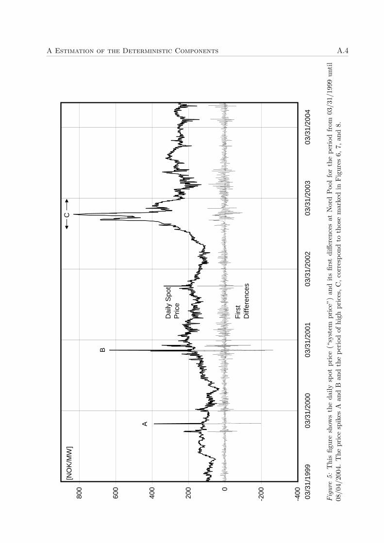
A Estimation of the Deterministic Components A.4
-400
-2000
200
400
600
800
03/3
1/19
9903
/31/
2000
03/3
1/20
0103
/31/
2002
03/3
1/20
0303
/31/
2004
[NO
K/M
W]
A
B
C
Firs
t D
iffer
ence
s
Dai
ly S
pot
Pric
e
Fig
ure
5:T
his
figur
esh
ows
the
daily
spot
pric
e(“
syst
empr
ice”
)an
dit
sfir
stdi
ffere
nces
atN
ord
Poo
lfo
rth
epe
riod
from
03/3
1/19
99un
til
08/0
4/20
04.
The
pric
esp
ikes
Aan
dB
and
the
peri
odof
high
pric
es,C
,co
rres
pond
toth
ose
mar
ked
inFig
ures
6,7,
and
8.
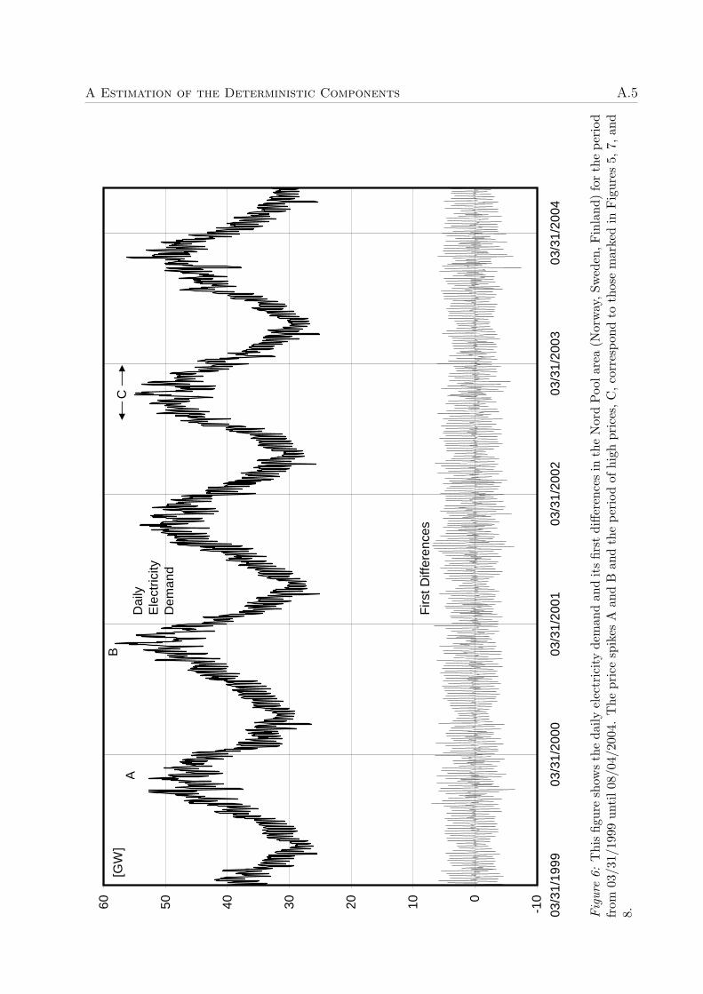
A Estimation of the Deterministic Components A.5
-100102030405060
03/3
1/19
9903
/31/
2000
03/3
1/20
0103
/31/
2002
03/3
1/20
0303
/31/
2004
[GW
]A
BC
Dai
ly
Ele
ctric
ity
Dem
and
Firs
t Diff
eren
ces
Fig
ure
6:T
his
figur
esh
ows
the
daily
elec
tric
ity
dem
and
and
its
first
diffe
renc
esin
the
Nor
dPoo
lare
a(N
orw
ay,S
wed
en,F
inla
nd)
for
the
peri
odfr
om03
/31/
1999
unti
l08/
04/2
004.
The
pric
esp
ikes
Aan
dB
and
the
peri
odof
high
pric
es,C
,cor
resp
ond
toth
ose
mar
ked
inFig
ures
5,7,
and
8.

A Estimation of the Deterministic Components A.6
0
200
400
600
800
2025
3035
4045
5055
60
Dai
ly S
pot P
rice
[NO
K/M
W]
Dai
ly E
lect
ricity
Dem
and
[GW
]
A
B
Fig
ure
7:T
his
figur
esh
ows
the
daily
spot
pric
ean
dth
eda
ilyde
man
din
asc
atte
rpl
otfo
rth
epe
riod
from
03/3
1/19
99un
til08
/10/
2004
.T
heco
rrel
atio
nbe
twee
nth
esp
otpr
ice
and
the
prod
ucti
onis
39.2
%,fo
rth
eir
first
diffe
renc
esit
is49
.7%
.T
hepo
ints
Aan
dB
corr
espo
ndto
thos
em
arke
din
Fig
ure
5an
d6.
The
data
poin
tsin
the
uppe
rle
ftar
eam
ostl
yco
rres
pond
toth
epe
riod
ofhi
ghpr
ices
,C,w
hich
isno
tm
arke
din
this
figur
e.
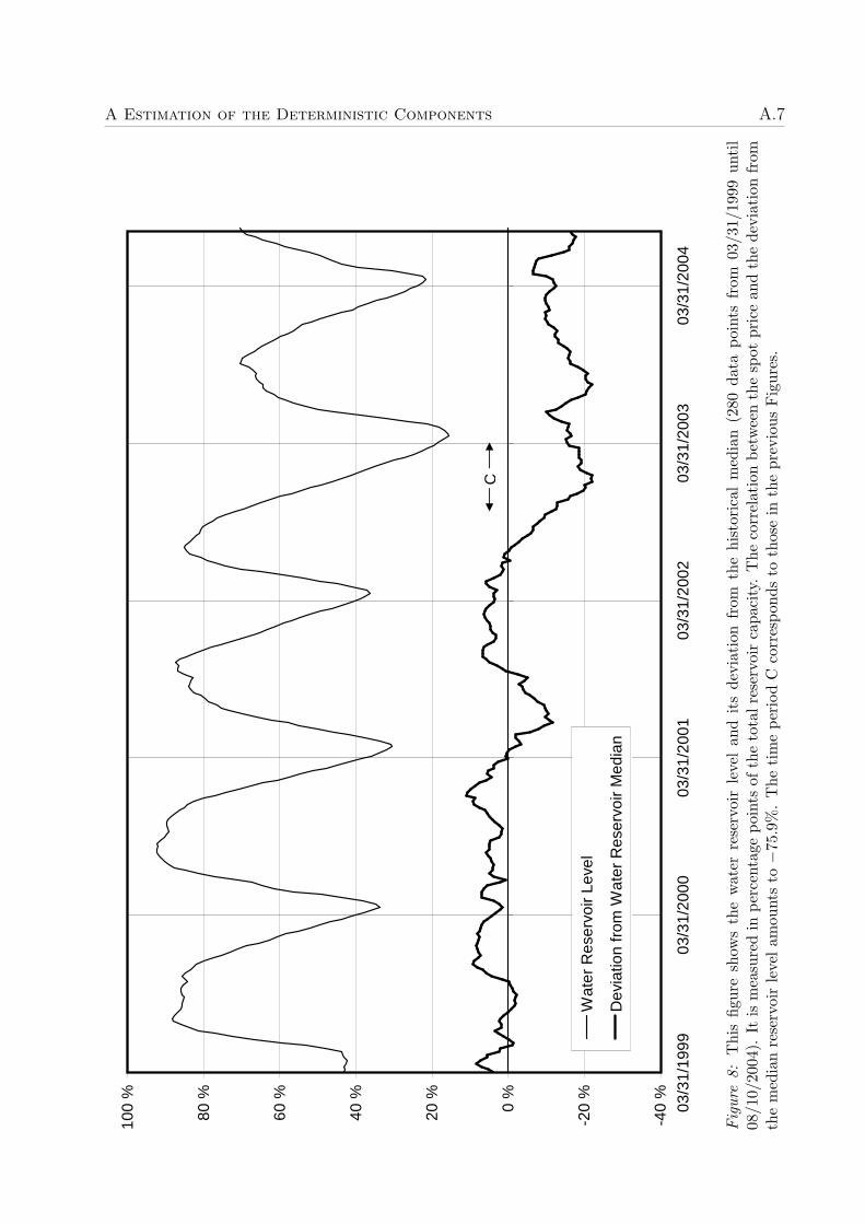
A Estimation of the Deterministic Components A.7
-40
%
-20
%
0 %
20 %
40 %
60 %
80 %
100
%
03/3
1/19
9903
/31/
2000
03/3
1/20
0103
/31/
2002
03/3
1/20
0303
/31/
2004
Wat
er R
eser
voir
Leve
l
Dev
iatio
n fr
om W
ater
Res
ervo
ir M
edia
n
C
Fig
ure
8:T
his
figur
esh
ows
the
wat
erre
serv
oir
leve
lan
dit
sde
viat
ion
from
the
hist
oric
alm
edia
n(2
80da
tapo
ints
from
03/3
1/19
99un
til
08/1
0/20
04).
Itis
mea
sure
din
perc
enta
gepo
ints
ofth
eto
talr
eser
voir
capa
city
.T
heco
rrel
atio
nbe
twee
nth
esp
otpr
ice
and
the
devi
atio
nfr
omth
em
edia
nre
serv
oir
leve
lam
ount
sto−7
5.9%
.T
heti
me
peri
odC
corr
espo
nds
toth
ose
inth
epr
evio
usFig
ures
.
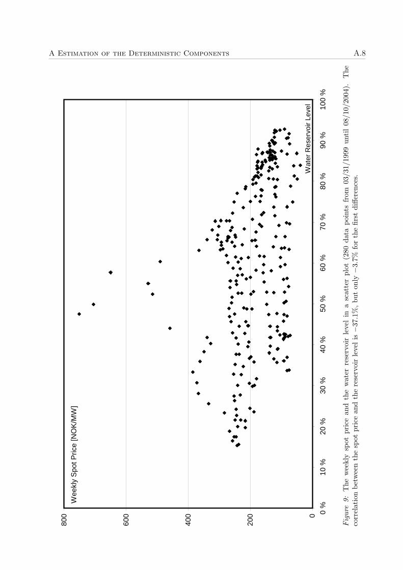
A Estimation of the Deterministic Components A.8
0
200
400
600
800 0
%10
%20
%30
%40
%50
%60
%70
%80
%90
%10
0 %
Wee
kly
Spo
t Pric
e [N
OK
/MW
]
Wat
er R
eser
voir
Leve
l
Fig
ure
9:T
hew
eekl
ysp
otpr
ice
and
the
wat
erre
serv
oir
leve
lin
asc
atte
rpl
ot(2
80da
tapo
ints
from
03/3
1/19
99un
til
08/1
0/20
04).
The
corr
elat
ion
betw
een
the
spot
pric
ean
dth
ere
serv
oir
leve
lis−3
7.1%
,bu
ton
ly−3
.7%
for
the
first
diffe
renc
es.

A Estimation of the Deterministic Components A.9
020
040
060
080
0
-25
%-2
0 %
-15
%-1
0 %
-5 %
0 %
5 %
10 %
Wee
kly
Spo
t Pric
e [N
OK
/MW
]
Dev
iatio
n fr
om W
ater
Res
ervo
ir M
edia
n
Fig
ure
10:
Thi
sfig
ure
show
sa
scat
ter
plot
ofth
ew
eekl
ysp
otpr
ice
and
the
wat
erre
serv
oir
devi
atio
nfr
omit
sm
edia
nin
%-p
oint
s(2
80da
tapo
ints
from
03/3
1/19
99un
til08
/10/
2004
).T
heco
rrel
atio
nbe
twee
nth
esp
otpr
ice
and
the
devi
atio
nfr
omth
ere
serv
oir
med
ian
is−7
5.9%
,fo
rth
efir
stdi
ffere
nces
itis−1
3.8%
.

A Estimation of the Deterministic Components A.10
-200
-1000
100
200
300
400
500
600
700
03/3
1/19
9903
/31/
2000
03/3
1/20
0103
/31/
2002
03/3
1/20
0303
/31/
2004
Dai
ly S
pot P
rice
Est
imat
ed D
eter
min
istic
Com
pone
nt
Res
idua
l
[NO
K/M
W]
Fig
ure
11:
Thi
sfig
ure
show
sth
eda
ilysp
otpr
ice,
Pt,
its
esti
mat
edde
term
inis
tic
com
pone
nt,f(t
),fo
rth
ere
duce
d-fo
rmm
odel
,an
dth
eda
ilyre
sidu
al(e
stim
atio
nw
indo
w:
11/0
1/19
96–0
8/04
/200
4).

A Estimation of the Deterministic Components A.11
-100102030405060
03/3
1/19
9903
/31/
2000
03/3
1/20
0103
/31/
2002
03/3
1/20
0303
/31/
2004
Dai
ly E
lect
ricity
Dem
and
Est
imat
ed D
eter
min
istic
Com
pone
nt
Res
idua
l
[GW
]
Fig
ure
12:
Thi
sfig
ure
show
sth
eda
ilyel
ectr
icity
dem
and
Dt,
its
esti
mat
edde
term
inis
tic
com
pone
ntD
tus
edin
the
equi
libri
umm
odel
,and
the
resi
dual
St(e
stim
atio
nw
indo
w:
03/2
9/19
99–0
8/04
/200
4).

A Estimation of the Deterministic Components A.12
0
100
200
300
400
500
600
700
800
2030
4050
6070
[NO
K/M
W]
D [G
W]
Fig
ure
13:
Thi
sfig
ure
show
sth
esc
atte
rpl
otof
wee
kly
aver
age
dem
and
Dtan
dth
ew
eekl
yav
erag
esp
otpr
ices
Ptdu
ring
the
obse
rvat
ion
peri
od.

A Estimation of the Deterministic Components A.13
0
100
200
300
400
500
600
700
800
2030
4050
6070
[NO
K/M
W]
D*
[GW
]
Fig
ure
14:
Thi
sfig
ure
show
sth
ees
tim
ated
mar
gina
lco
stfu
ncti
onC′ (D∗ )
=ex
p(4.
64+
0.02
09D∗ )
whe
reD∗
=D−
0.44
98W
RD
)an
dth
esc
atte
rpl
otof
the
adju
sted
dem
and
D∗
and
the
wee
kly
aver
age
spot
pric
es.
The
para
met
ers
ofth
em
argi
nalc
ost
func
tion
are
esti
mat
edon
the
full
obse
rvat
ion
peri
od,i.
e.th
efig
ure
show
san
in-s
ampl
eco
mpa
riso
n.
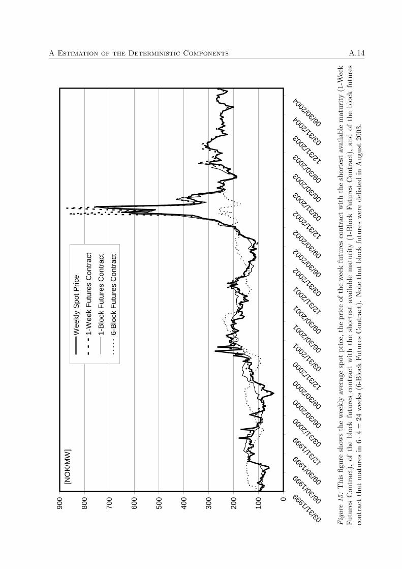
A Estimation of the Deterministic Components A.14
0
100
200
300
400
500
600
700
800
900
03/3
1/19
99 06/3
0/19
99 09/3
0/19
99 12/3
1/19
99 03/3
1/20
00 06/3
0/20
00 09/3
0/20
00 12/3
1/20
00 03/3
1/20
01 06/3
0/20
01 09/3
0/20
01 12/3
1/20
01 03/3
1/20
02 06/3
0/20
02 09/3
0/20
02 12/3
1/20
02 03/3
1/20
03 06/3
0/20
03 09/3
0/20
03 12/3
1/20
03 03/3
1/20
04 06/3
0/20
04
Wee
kly
Spo
t Pri
ce
1-W
eek
Fut
ures
Con
trac
t
1-B
lock
Fut
ures
Con
trac
t
6-B
lock
Fut
ures
Con
trac
t
[NO
K/M
W]
Fig
ure
15:
Thi
sfig
ure
show
sth
ew
eekl
yav
erag
esp
otpr
ice,
the
pric
eof
the
wee
kfu
ture
sco
ntra
ctw
ith
the
shor
test
avai
labl
em
atur
ity
(1-W
eek
Futu
res
Con
trac
t),
ofth
ebl
ock
futu
res
cont
ract
wit
hth
esh
orte
stav
aila
ble
mat
urity
(1-B
lock
Futu
res
Con
trac
t),
and
ofth
ebl
ock
futu
res
cont
ract
that
mat
ures
in6·4
=24
wee
ks(6
-Blo
ckFu
ture
sC
ontr
act)
.N
ote
that
bloc
kfu
ture
sw
ere
delis
ted
inA
ugus
t20
03.

A Estimation of the Deterministic Components A.15
050100
150
200
250
05/2
9/02
Wee
k 2W
eek 4
Wee
k 6Bloc
k 1
Block 2
Block 3
Block 4
Block 5
Block 6
Block 7
Block 8
Block 9
Block 1
0
Obs
erve
d F
utur
es P
rices
L/S
, Ris
k N
eutr
al F
utur
es P
rices
L/S
, Fut
ures
Pric
es w
ith Im
plic
it R
isk
Pre
miu
m
L/S
, Im
plic
it R
isk
Pre
miu
m
Eq.
, Ris
k N
eutr
al F
utur
es P
rices
Eq.
, Fut
ures
Pric
es w
ith Im
plic
it R
isk
Pre
miu
m
Eq.
, Im
plic
it R
isk
Pre
miu
m
[NO
K/M
W]
Fig
ure
16:
Thi
sfig
ure
show
sth
eob
serv
edfu
ture
scu
rve,
the
theo
reti
calfu
ture
scu
rves
and
the
theo
reti
calfu
ture
spr
emia
at05
/29/
2002
.T
hegr
eyse
ctio
nsof
the
obse
rved
futu
res
curv
ede
note
sett
lem
ent
pric
esth
atw
ere
not
trad
edan
dth
usno
tco
nsid
ered
inth
eim
plic
ites
tim
atio
nof
risk
para
met
ers.

A Estimation of the Deterministic Components A.16
-200
-1000
100
200
300
400
500
600
3-M
ay-0
028
-Jun
-00
23-A
ug-0
018
-Oct-
00 13-D
ec-0
0 7-Feb
-01 4-
Apr-0
130
-May
-01 25
-Jul-
01 19-S
ep-0
114
-Nov
-01 9-
Jan-
02 6-M
ar-0
2 1-M
ay-0
226
-Jun
-02
21-A
ug-0
216
-Oct-
02 11-D
ec-0
2 5-Feb
-03 2-
Apr-0
328
-May
-03 23
-Jul-
03 17-S
ep-0
312
-Nov
-03 7-
Jan-
04 3-M
ar-0
428
-Apr
-04
23-J
un-0
4
MA
D R
educ
ed-f
orm
Mod
elM
D R
educ
ed-f
orm
Mod
elM
AD
Equ
ilibr
ium
Mod
elM
D E
qulib
rium
Mod
elA
vera
ge S
pot P
rice
[NO
K]
Fig
ure
17:
Thi
sfig
ure
show
sth
eM
AD
and
the
MD
for
both
mod
els
inth
eca
seof
risk
neut
ralit
y(λ
=0,
ξ=
0)an
dth
e8-
wee
kav
erag
esp
otpr
ice.

A Estimation of the Deterministic Components A.17
-160
0
-140
0
-120
0
-100
0
-800
-600
-400
-2000
200
05
1015
2025
3035
4045
50
[NO
K]
Tim
e to
Mat
urity
[wee
ks]
Fig
ure
18:
Thi
sFig
ure
show
sa
scat
ter
plot
ofth
ein
-sam
ple
esti
mat
edri
skpr
emia
ofth
ere
duce
d-fo
rmm
odel
alon
gth
eti
me
tom
atur
ity.

A Estimation of the Deterministic Components A.18
-100-5
0050100
150
200
250
05
1015
2025
3035
4045
50
Tim
e to
Mat
urity
[wee
ks]
[NO
K]
Fig
ure
19:
Thi
sFig
ure
show
sa
scat
ter
plot
ofth
ein
-sam
ple
esti
mat
edri
skpr
emia
ofth
eeq
uilib
rium
mod
elal
ong
the
tim
eto
mat
urity.

A Estimation of the Deterministic Components A.19
-1
-0.50
0.51
1.5
3-M
ay-0
028
-Jun
-00
23-A
ug-0
018
-Oct-
00 13-D
ec-0
0 7-Feb
-01 4-
Apr-0
130
-May
-01
25-J
ul-01 19
-Sep
-01
14-N
ov-0
1 9-Ja
n-02 6-
Mar
-02
1-M
ay-0
226
-Jun
-02
21-A
ug-0
216
-Oct-
02 11-D
ec-0
2 5-Feb
-03 2-
Apr-0
328
-May
-03
23-J
ul-03 17
-Sep
-03
12-N
ov-0
3 7-Ja
n-04 3-
Mar
-04
28-A
pr-0
423
-Jun
-04
0100
200
300
400
500
λ ξ Ave
rage
Spo
t Pric
e (r
ight
sca
le)
. 103
Fig
ure
20:
Thi
sfig
ure
show
sth
eim
plic
itly
esti
mat
edλ
and
ξof
the
redu
ced-
form
mod
elan
dth
eeq
uilib
rium
mod
el,re
spec
tive
ly.
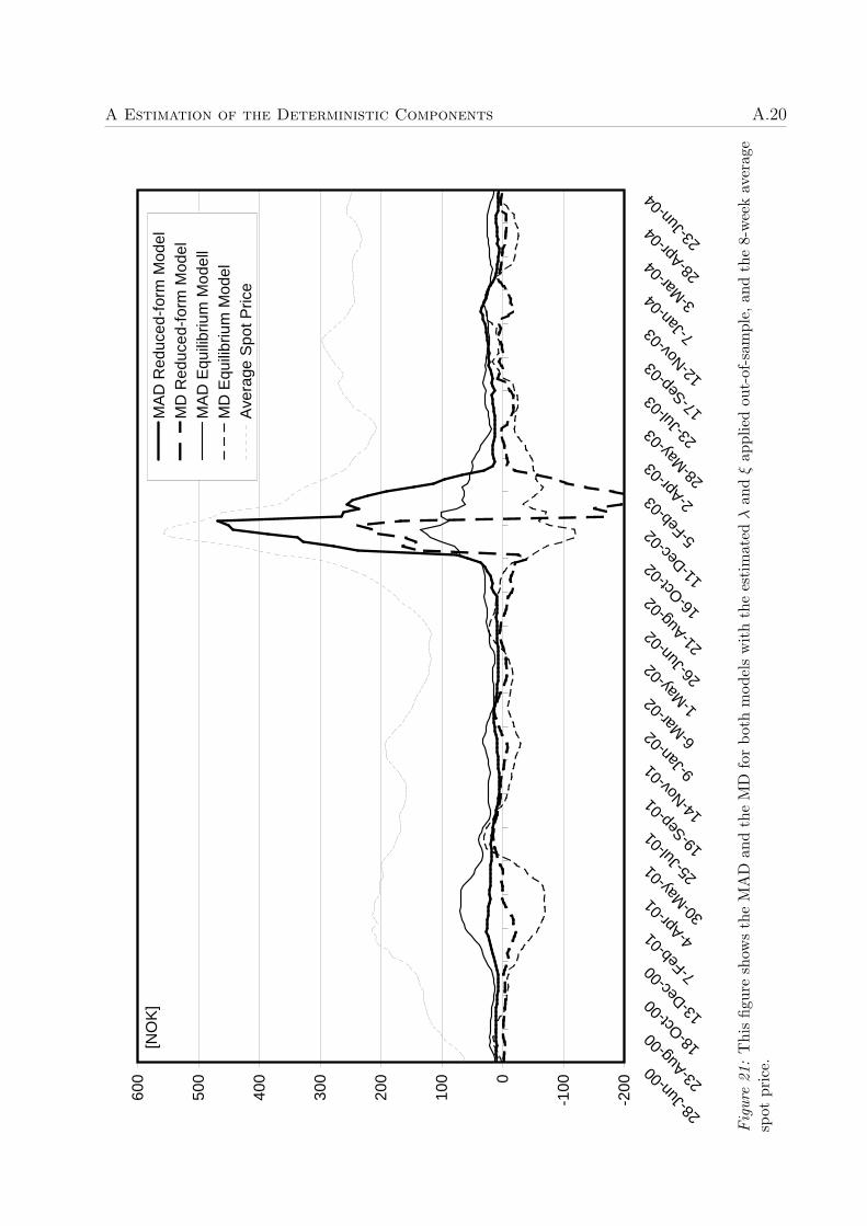
A Estimation of the Deterministic Components A.20
-200
-1000
100
200
300
400
500
600
28-J
un-0
023
-Aug
-00
18-O
ct-00 13
-Dec
-00 7-
Feb-0
1 4-Apr
-01
30-M
ay-0
1 25-J
ul-01 19
-Sep
-01
14-N
ov-0
1 9-Ja
n-02 6-
Mar
-02 1-
May
-02
26-J
un-0
221
-Aug
-02
16-O
ct-02 11
-Dec
-02 5-
Feb-0
3 2-Apr
-03
28-M
ay-0
3 23-J
ul-03 17
-Sep
-03
12-N
ov-0
3 7-Ja
n-04 3-
Mar
-04
28-A
pr-0
423
-Jun
-04
MA
D R
educ
ed-f
orm
Mod
elM
D R
educ
ed-f
orm
Mod
elM
AD
Equ
ilibr
ium
Mod
ell
MD
Equ
ilibr
ium
Mod
elA
vera
ge S
pot P
rice
[NO
K]
Fig
ure
21:
Thi
sfig
ure
show
sth
eM
AD
and
the
MD
for
both
mod
els
wit
hth
ees
tim
ated
λan
dξ
appl
ied
out-
of-s
ampl
e,an
dth
e8-
wee
kav
erag
esp
otpr
ice.