Embed Size (px)
Citation preview

43
ON THE
VALUATION OF
CORPORATE BONDS
by
Edwin J. Elton,* Martin J. Gruber,*
Deepak Agrawal** and Christopher Mann**
* Nomura Professors, New York University
** Doctoral students, New York University

1
The valuation of corporate debt is an important issue in asset pricing. While there has
been an enormous amount of theoretical modeling of corporate bond prices, there has been
relatively little empirical testing of these models. Recently there has been extensive development
of rating based models as a type of reduced form model. These models take as a premise that
groups of bonds can be identified which are homogeneous with respect to risk. For each risk
group the models require estimates of several characteristics such as the spot yield curve, the
default probabilities and the recovery rate. These estimates are then used to compute the
theoretical price for each bond in the group. The purpose of this article is to clarify some of the
differences among these models, to examine how well they explain prices, and to examine how
to group bonds to most effectively estimate prices.
This article is divided into four sections. In the first section we explore two versions of
rating-based models emphasizing their differences and similarities. The first version discounts
promised cash flows at the spot rates that are estimated for the group in question. The second
version uses estimates of risk-neutral default probabilities to define a set of certainty equivalent
cash flows which are discounted at estimated government spot rates to arrive at a model price.
The particular variant of this second model we will use was developed by Jarrow, Lando and
Turnbull (1997). In the second section of this paper we explore how well these models explain
actual prices. In this section we accept Moody’s ratings along with classification as an industrial
or financial firm as sufficient metrics for grouping. In the next section, we examine what
additional characteristics of bonds beyond Moody’s classification are useful in deriving a

2
homogeneous grouping. In the last section we examine whether employing these characteristics
can increase the precision with which we can estimate bond prices.
I. Alternative Models:
There are two basic approaches to the pricing of risky debt: reduced form models, of
which rating based models are a sub class, and models based on option pricing. Rating-based
models are found in Elton, Gruber, Agrawal, and Mann (1999), Duffie and Singleton (1997),
Jarrow, Lando and Turnbull (1997), Lando (1997), Das and Tufano (1996). Option-based models
are found in Merton (1974) and Jones and Rosenfeld (1984). In this paper we will deal with a
subset of reduced form models, those that are ratings based. Discussion of the efficacy of the
second approach can be found in Jones and Rosenfeld (1984).
We now turn to a discussion of the two versions of rating-based models which have been
advocated in the literature of Financial Economics and to a comparison of the bond valuations
they produce. The simplest version of a rating-based model first finds a set of spot rates that best
explain the prices of all corporate bonds in any rating class. It then finds the theoretical or model
price for any bond in this rating class by discounting the promised cash flows at the spot rates
estimated for the rating class. We refer to this approach as discounting promised payments or
DPP model. The idea of finding a set of risky spots that explain corporate bonds of a
homogeneous risk class has been used by Elton, Gruber, Agrawal and Mann (1999). While there
are many ways to justify this procedure, the most elegant is that contained in Duffie and

1 As shown in Elton, Gruber, Agrawal and Mann (1999), state taxes affect corporatebond pricing. The estimated risk-neutral probability rates are estimated using spot rates. Sincespot rates include the effect of state taxes. These tax effects will be impounded in risk-neutralprobabilities.
3
Singleton (1997). They delineate the conditions under which these prices are consistent with no
arbitrage in the corporate bond market. We refer to the DPP model as a rating based model
under the reduced form category because, as shown in the appendix, DPP is equivalent to a
model which uses risk neutral default probabilities (and a particular recovery assumption) to
calculate certainty equivalent cash flows which are then discounted at riskless rates. To find the
bonds model price the recovery assumption necessary for this equivalency is that at default the
investor recovers a fraction of the market value of an equivalent corporate bond plus its coupon.
The second version of a rating-based model is the particular form of the risk-neutral
approach used by Jarrow, Lando and Turnbull (1997), and elaborated by Das (1999) and Lando
(1999). This version, referred to hereafter as JLT, like all rating based models involves
estimating a set of risk-neutral default probabilities which are used to determine certainty
equivalent cash flows which in turn can be discounted at estimated government spot rates to find
the model price of corporate bonds1. Unlike DPP, the JLT requires an explicit estimate of risk
neutral probabilities. To estimate risk neutral probabilities JLT start with an estimate of the
transition matrix of bonds across risk classes (including default), an estimate of the recovery rate
in the event of default, estimates of spot rates on government bonds and estimates of spot rates
on zero coupon corporate bonds within each rating class. JLT select the risk-neutral probabilities
so that for zero coupon bonds, the certainty equivalent cash flows discounted at the riskless spot

2 Many discussions of the JLT models describe this assumption as the recovery ofan equivalent treasury. The equivalence occurs because all cash flows are discounted at thegovernment bond spot rates.
4
rates have the same value as discounting the promised cash flows at the corporate spot rate. In
making this calculation, any payoff from default, including the payoff from early default, is
assumed to occur at maturity and the amount of the payoff is a percentage of par. This is
mathematically identical to assuming that at the time of default a payment is received which is
equal to a percentage of the market value of a zero coupon government bond of the same
maturity as the defaulting bond.2 Thus, one way to view the DPP and JLT models is that they are
both risk neutral models but they make different recovery assumptions.
A. Comparison for zero coupon bonds
In this section we will show that for zero coupon bonds, the JLT and DPP procedures are
identical. We will initially derive the value of a bond using the JLT procedure.
To see how these models compare, we defined the following symbols:
1. be the actual transition probability matrix.Q

5
2. be the actual probability of going from rating class i to default sometime over tq tid ( )
periods and is the appropriate element of .Qt
3. be the probability risk adjustment for the tth period for a bond initially in ratingΠ i t( )
class i.
4. be the risk adjusted (neutral) probability of going from rating class i to default atA ti ( )
some time over t periods. It is equal to .Π i idt q t( ) ( )
5. be the price of a bond in rating class i at time zero that matures at time T. ViT
6. be the government spot rate at time zero that is appropriate for discounting cashr tg
0
flows received at time t.
7. be the corporate spot rate at time zero appropriate for discounting the cash flow atr tci
0
time t on a bond in risk category i.

6
8. be the fraction of the face value for a bankrupt bond that is paid to the holder of abi
corporate bond in class i at the maturity.
Since zero coupon bonds have cash flows only at maturity and since, for JLT model, recovery is
assumed to occur at maturity, we have only one certainty equivalent cash flow to determine. As
shown in Das (1999) or Lando (1999), the probability risk adjustment for this cash flow in the
JLT model is
Π iTg
Tci
T
i idT
rr b q T
( )( ) ( )
= −++
� ��
���
�� −
111
11
0
0
Multiplying both sides of equation (1) by we find that is equal toq Tid ( ), A Ti ( )
(1)( )( ) ( )A T
r
r biTg T
Tci T
i
( ) = −+
+��
�� −
11
11
10
0

3 This also follows directly from noting that their results are equivalent todiscounting promised cash flows at spot rates.
4 Thus if bond pricing is the purpose of the analysis, the various estimationtechniques developed for estimating transition matrixes are vacuous in that they lead to identicalpricing. See Lando (1997)for a review of these techniques.
7
From examining the right-hand side of the equation, is independent of the value ofA Ti ( )
Thus unlike JLT’s assertion, risk-adjusted probabilities are not a function of transitionq Tid ( ).
probabilities and , the results of their analysis are completely independent of the transition matrix
used to price bonds.3 Risk-adjusted probabilities are only a function of the spot rates on
governments, the spot rates on corporates, and the recovery rate.4
The risk-neutral price of a zero coupon corporate bond maturing after T periods in rating
class i where any payment for default is made at maturity is given by:
(2)( )VA T b A T
riTz i i i
Tg T=
− +
+
100 1 1001 0
( ( )) ( )
where the superscript Z has been added to to explicitly recognize that this equation holdsViT
only for zero coupon bonds. Substituting (1) into (2) yields

8
(3)( )VriT
z
Tci T=
+100
1 0
Thus, as stated earlier, employing the JLT methodology yields exactly the same model
price for any zero coupon bond (where payment for default only occurs at maturity) as
discounting the promised cash flow at the corporate spot rates that were used as input to the
analysis. If the only bonds we were interested in were zero coupon bonds where payment for
default occurred at maturity, it would not matter in terms of pricing bonds whether we discounted
promised payments at the corporate spot rate or used the JLT procedure. Why, then, bother with
both models? The reason is that they produce very different answers if we examine coupon-
paying bonds, or in fact any bond where the pattern of cash flows in any period is different from
that of a zero coupon bond that pays off as a percentage of par in default at the horizon.
B. Comparison for Coupon Bonds
If we examine a two-period bond with a coupon of c dollars, the value of the bond using
the corporate spot rate to discount promised payments is
(4)( ) ( )Vcr
cr
i ci ci201 02
21100
1=
++
+
+

5 JLT assume that at bankruptcy the investor recovers a fraction of the face value ofthe bond at the horizon or equivalently an amount equal to the fraction of an equal maturitygovernment bond at the time of bankruptcy. In the appendix we show that if an investor recoversan amount equal to a fraction of the market value of an equal maturity corporate bond in the samerisk class plus the same fraction of the coupon, then the risk-neutral valuation gives the samevaluation as discounting promised cash flows at corporate spot rates.
6 This is the procedure employed by JLT. An alternative might be to solve for thefactor that produced the same value for a bond with an average coupon. However, since the
9
Using risk-adjusted probabilities and continuing the assumption that the recovery of cash
flows on defaulted bonds occurs at the maturity of the bond.5
(5)( )( )[ ]( )V
c Ar
c A b A
ri
ig
i i i
g201 02
21 11
100 1 2 100 2
1=
−+
++ − +
+
( ( )) ( ) ( ) ( )
It is easy to see that these two equations (4) and (5) are not equal to each other for the
definition of risk adjustment given by equation (1), and in fact that there is no risk-adjustment
expression that will equate them for a group of coupon paying bonds with different coupons
using JLT’s assumption about recovery.
However, we can be more precise concerning the direction of the differences. We will
now show that the JLT procedure will produce model prices which are lower for coupon paying
debt than those produced by discounting promised cash flows at corporate spot rates. The JLT
risk adjustment factor was arrived at by finding the factor that produced the same value for zero
coupon debt as discounting promised cash flows at the corporate spot rate.6

correct factor in the JLT procedure is a function of coupon, this would misprice bonds in amanner analogous to that shown in the following analysis.
7 All our empirical work uses continuous compounding. However, it is easier tofollow the discussion, and the comparisons are more obvious, using discrete compounding.
10
The risk-neutral valuation of zeros is
( )( )V
A T b A TiTz i i i
TT=
− +1 100 100( ) ( )
1+ r0g
The valuation from discounting promised cash flows is
( )VriT
z
Tci T=
+
1001 0
Equating the two and solving for 7A Ti ( )
(6)( )( ) ( )A T
r
r biTg T
Tci T
i
( ) = −+
+��
�� −
11
11
10
0

11
Note this is identical to the definition of from Das (1999) and Lando (1999) presentedA Ti ( )
earlier.
If there was a coupon in the last period, the present value of the last period’s cash flow
would be
( )( )( )v
A T c b A T
riTi i i
OTg T=
− + +
+
1 100 100
1
( ) ( )
Where the lower case v indicates it is the present value of a single cash flow rather than the
complete bond value.
Discounting the last period’s promised cash flow at the corporate spot rate yields
( )vc
riT
Tc T=
+
+
1001 0
Equating these two equations and solving for yieldsA Ti ( )

12
(7)( )( )A T
r
r bc
iTg T
Tci T
i
( ) = −+
+��
��
−+
���
��
11
11
1100
100
0
0
If we examine the cash flows for any period prior to the period in which a bond matures,
the present value of the tth period cash flow using risk-neutral probabilities is
( )( )v
A t c
riti
tg t=
−
+
1
1 0
( )
and for promised cash flows the present value of the tth period cash flow is
( )vcrit
tci t=
+1 0
Equating and solving for yieldsA ti ( )
(8)( )( )A t
r
ritg t
tci t( ) = −
+
+��
��1
1
10
0
8 See Duffie and Singleton (1997) for a detailed discussion of assumptions underwhich it is exactly correct to discount promised payments at spot rates. See Appendix A for adiscussion of the recovery assumption necessary for discounting promised cash flows at the spotrate to be the same as risk-neutral valuation.
13
By inspection, equation (6) results in a higher value for any than equation (7) orA ti ( )
(8). Thus using zeros to define under the JLT procedure leads to estimates of thatA ti ( ) A ti ( )
are larger than those obtained by determining using coupon paying bonds. From equationA ti ( )
(5) using higher results in lower prices. Thus using the JLT procedure will always resultA t si ( )'
in lower estimated prices than discounting promised cash flows at corporate spot rates. Later we
will estimate and examine the size of this difference for coupon paying corporate bonds.
Since the JLT methodology leads to different values for coupon-paying corporate debt
than discounting promised cash flows at corporate spot rates, the question remains as to which
provides more accurate valuation. Discounting promised payments at corporate spot rates is an
approximation except under restrictive conditions. The defense of using spots is an arbitrage
argument, and the arbitrage argument in terms of promised payments is an approximation which
is only exactly correct under certain assumptions.8 On the other hand, the structure of the JLT
model insures that coupon paying bond prices can’t be reproduced exactly even over a fit period.
The choice between these models then becomes an empirical matter, one to which we now turn.
II. TESTING THE MODELS
9 The only difference in the way CRSP data is constructed and our data isconstructed is that over the period of our study CRSP used an average of bid/ask quotes from fiveprimary dealers called randomly by the New York Fed rather than a single dealer. However,comparison of a period when CRSP data came from a single dealer and also from the five dealerssurveyed by the Fed showed no difference in accuracy (Sarig and Warga, (1989)). See also thediscussion of pricing errors in Elton, Gruber, Agrawal and Mann (1999).Thus our data should becomparable in accuracy to the CRSP data.
14
A. DATA
Our bond data is extracted from the Lehman Brothers Fixed Income database distributed
by Warga (1998). This database contains monthly price, accrued interest, and return data on all
investment grade corporate and government bonds. In addition, the database contains descriptive
data on bonds including coupon, ratings, and callability.
A subset of the data in the Warga database is used in this study. First, any bond that is
matrix-priced rather than trader-priced in a particular month is eliminated from the sample for
that month. Employing matrix prices might mean that all our analysis uncovers is the formula
used to matrix price bonds rather than the economic influences at work in the market.
Eliminating matrix priced bonds leaves us with a set of prices based on dealer quotes. This is the
same type of data contained in the standard academic source of government bond data: the CRSP
government bond file.9

10 Slightly less than 3% of the sample was eliminated because of problematic data.The eliminated bonds had either a price that was clearly out of line with surrounding prices(pricing error) or involved a company or bond undergoing a major change.
15
Next, we eliminate all bonds with special features that would result in their being priced
differently. This means we eliminate all bonds with options (e.g., callable or sinking fund), all
corporate floating rate debt, bonds with an odd frequency of coupon payments, government
flower bonds and index-linked bonds. Next, we eliminate all bonds not included in the Lehman
Brothers bond indexes because researchers in charge of the database at Shearson-Lehman
indicated that the care in preparing the data was much less for bonds not included in their
indexes. Finally, we eliminate bonds where the data is problematic.10 For classifying bonds we
use Moody’s ratings. In the few cases where Moody’s ratings do not exist, we classify using the
equivalent S&P rating.
B. Testing the Approaches
In this section we discuss the comparison of model errors produced by discounting
promised cash flows at corporate spot rates with those produced by discounting risk-adjusted
cash flows at the riskless government rates.
Calculating model prices using the discounting of promised cash flows is relatively
straightforward. First, spots rates must be calculated. In order to find spot rates, we used the
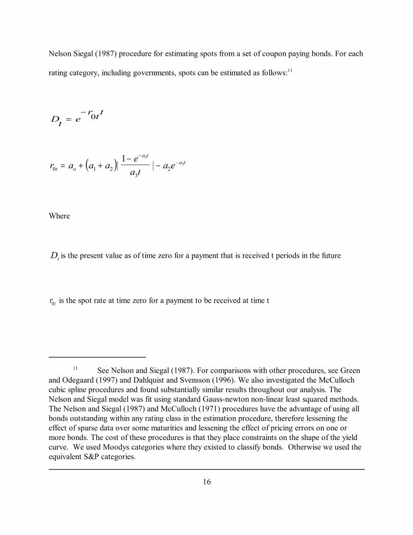
11 See Nelson and Siegal (1987). For comparisons with other procedures, see Greenand Odegaard (1997) and Dahlquist and Svensson (1996). We also investigated the McCullochcubic spline procedures and found substantially similar results throughout our analysis. TheNelson and Siegal model was fit using standard Gauss-newton non-linear least squared methods.The Nelson and Siegal (1987) and McCulloch (1971) procedures have the advantage of using allbonds outstanding within any rating class in the estimation procedure, therefore lessening theeffect of sparse data over some maturities and lessening the effect of pricing errors on one ormore bonds. The cost of these procedures is that they place constraints on the shape of the yieldcurve. We used Moodys categories where they existed to classify bonds. Otherwise we used theequivalent S&P categories.
16
Nelson Siegal (1987) procedure for estimating spots from a set of coupon paying bonds. For each
rating category, including governments, spots can be estimated as follows:11
Dt er tt=
−0
( )r a a ae
a ta et o
a ta t
0 1 23
2
1 3
3= + +−
� � −−
−
Where
is the present value as of time zero for a payment that is received t periods in the futureDt
is the spot rate at time zero for a payment to be received at time tr t0

12 For a discussion of historical rates see Elton, Gruber, Agrawal and Mann (1999). We us continuous compounding in estimating risk neutral possibilities.
17
are parameters of the modela a a a0 1 2 3, , and
Discounting the promised cash flows at these estimated rates produces the model prices
for this technique.
The estimation for the JLT procedure is more complicated. The first step is to estimate
risk-neutral probabilities based on equation (1). So that the models can be directly compared, we
use the same estimated spots that were used to discount promised cash flows as input to equation
(1). We used historical recovery rates for Aa, A, and Baa rated corporate bonds.12
In Table I we report the risk-adjusted probabilities we arrive at using this procedure.
While risk-adjusted probabilities are derived each month, in the interest of brevity we report
them once a year (January) for each year in our sample period and only for industrial Baa bonds.
It is interesting that the risk-neutral probabilities we arrive at are quite well-behaved relative to
the risk-neutral probabilities reported by other authors (e.g., Jarrow, Lando, Turnbull (1997). In
particular, our risk-neutral probabilities are all positive, and increase with maturity. We attribute
the greater plausibility of our results to the large sample we use as well as the procedure we
employ to extract spot rates.

18
As shown earlier, if one uses the JLT model, the risk-adjusted probabilities from zero
coupon bonds should understate the price of any coupon-paying bond. In addition, we would
expect that the absolute errors (a measure of dispersion) should be higher for the errors
themselves should be function of the coupon and coupons vary within any rating class.
Table II shows that the empirical results are consistent with the implications of the theory.
Note, as shown in Table II Panel A, that when bonds are priced by discounting promised
payments at corporate spot rates, the average error for each class of bonds is very close to zero
and overall the average error is less than one cent per $100 bond. When we look at the average
pricing errors from the JLT procedure, we see that they are negative and quite large for any class
of bonds. Errors are measured as JLT model price minus invoice price. The negative error shows
that the JLT procedure applied to coupon-paying bonds understates their market value. In
addition, as shown in Table II Panel B the average absolute error is much higher for the JLT
procedure. The average absolute error is affected by both the mean error and the dispersion
across bonds. Table 2C corrects for the mean error by computing the average absolute error
around the mean. Since the average error for DPP is close to zero, this correction has little effect
on DPP and the average absolute errors in 2B and 2C are similar. Since there is a large mean
error for JLT, calculating average absolute errors around the mean does make a difference for
JLT. Even after this correction, however, absolute JLT errors are much higher than absolute DPP
errors. Thus, the JLT procedure not only has a mean bias, but also results in greater dispersion of
errors around the mean across bonds. These results are exactly what our analytical examination
of the models lead us to expect.

19
It is worth examining one more point before we end this section. We would not expect
the average error to be a function of maturity when we discount promised payments. With the
JLT procedure we would expect the error to increase as maturity increases. This pattern occurs
because each coupon is systematically undervalued and the more coupons a bond pays, the larger
the mispricing. This is exactly what happens, as shown in Table III. For example, for the JLT
procedure applied to BBB industrial bonds, the error increases from thirteen cents per $100 to
over $3 per $100 as maturity increases.
In the next section of this paper we examine the ability of additional bond and/or
company characteristics to improve the pricing of corporate bonds. We will conduct this
examination employing the model which discounts promised cash flows at a rate which is
appropriate for the risk of the promised payments rather than the JLT model since it produced
lower errors.
III. Getting a Homogeneous Sample
When estimating spot rates, one has to make a decision as to how to construct a group of
bonds that is homogeneous with respect to risk. In the prior section we accepted the major
classifications of rating agencies. In this section we explore the use of additional data to form
more meaningful groups.

20
In general, when dividing bonds into subsets, one faces a difficult tradeoff. The more
subsets one has, the less bonds are present in any subset. Bond prices are subject to idiosyncratic
noise as well as systematic influences. The more bonds in a subset, the more the idiosyncratic
noise is averaged out. This suggests larger groupings. However, if the subset is not
homogeneous, one may be averaging out important differences in underlying risk and mis-
estimating spot rates because they are estimated for a group of bonds where subsets of the group
have different yield curves.
What are the characteristics of bonds that vary within a rating class that could lead to
price differences? We will examine the following possibilities:
(A) Default risk
(B) Liquidity
(C) Tax liability
(D) Recovery rates
(E) Age
A. Differential Default Risks:

13For all bonds rated by Moodys we use Moodys’ classification. For the few bonds notrated by Moody’s, we use S&P’s classification.
21
All bonds within a rating class may not be viewed as equally risky. There are several
characteristics of bonds which might be useful in dividing bonds within a rating class into new
groups. We will examine several of these in this section. We start by examining the subcategories
of risk within a rating class which Moodys and Standard & Poors have both introduced. We then
examine whether either past changes in rating category or a difference in rating by Standard &
Poors and Moodys convey information.
We start by examining the finer breakdown of ratings produced by the rating agencies
themselves. Standard & Poors and Moodys have introduced plus and minus categories within
each letter rating class. One obvious possibility is that bonds that are rated as a plus or a minus
are viewed as having different risk than bonds that receive a flat letter rating. If this is true, then
estimating one set of spot rates for all bonds in a class should result in consistent pricing errors
for bonds rated “plus” (too low a model price and hence negative errors) or bonds rated “minus”
(too high a model price and hence positive errors).
Tables IVA and IVB explore this possibility. For each rating class the table is split into
two sections. The top section shows the number of bond months in each rating class for varying
maturity and across all maturities.13 The bottom section shows the average of the model price
minus the invoice price (market price plus accrued interest) for each rating category. For all
rating categories, plus-rated bonds have, on average, too low a model price, and minus-rated

22
bonds too high a model price. The difference between the pricing error of plus rated, flat, and
negative rated bonds is statistically significant at the 5% level. Furthermore, the differences are
of economic significance (e.g., for minus versus flat Baa industrial bonds the difference is almost
1% of the invoice price). The same pattern is present for most of the maturities. In addition, the
size of the average pricing error increases as rating decreases. Thus, it is most important for Baa
bonds. This would suggest that one should estimate a separate spot curve for these subclasses of
ratings. However, for much of the sample, the paucity of bonds in many of the subclasses makes
it difficult to estimate meaningful spot rates for a subclass. Instead, we propose to directly
estimate the price impact of the finer gradation of rankings on errors (which is a function of
maturity). The ability to correct the model price for these differences will be examined in the
next section.
There is a second reason why investors might consider bonds within the same rating class
to have different risk. Investors might believe that a particular bond is likely to be downgraded or
upgraded. One predictor of this might be past rating changes. Past rating changes might predict
future rating changes, either because rating agencies tended to make changes in steps or because
a company whose risk has increased or decreased in the past is more likely to experience similar
changes in the future. In Table V we explore whether past rating changes contain information
about future rating changes. As shown in the table, bonds that have been upgraded in the past are
more than twice as likely to be upgraded in the future than they are to be downgraded, and bonds
that have been downgraded in the past are about twice as likely to be downgraded than upgraded
in the future.

23
Although there is evidence that past rating changes predict future rating changes, it is
unclear if the tendency is strong enough to show up in price data. We examined differences
between model price and invoice price for all bonds which had a past change in ratings. Pricing
errors were examined in the month of the change, the next three months after the change, and the
period 4 to 15 months after the change. These results are shown in Table VI. Despite the fact that
past rating changes contain information about future rating changes, we find no evidence that
bonds with past rating changes have prices that are systematically different from model prices.
Our sample of bonds with rating changes was quite small, for there were few bonds which had
rating changes. Thus the failure to find a relationship between past rating changes and errors
could arise either because investors do not take the predictability of past rating changes into
account when they price bonds, or simply because the number of rating changes is so small that
the effect is swamped by random pricing errors. In any case, examining past rating changes
provides no evidence that the Markoff assumption used in calculating the transition probability
matrix found in many studies is violated.
In Table VII we explore whether bonds that are given a higher (lower) rating by S&P than
by Moody’s are considered less (more) risky by investors. In considering differences we use
pluses and minuses. Thus, if Moodys rates a bond as Baa and S&P rates the bond BBB+, we
count this as a difference in ratings. Once again the upper half of the table shows the number of
bonds in each category, and the lower half the difference between model price and invoice price.
In presenting the data we do not sub-classify by maturity since we found no pattern in pricing
errors across maturity.

24
Investors clearly take the difference in rating into account. If the S&P rating is lower than
Moodys, then investors act as if the bond is higher risk than is implied by the Moodys rating and
they will set a lower market price, and this results in a model price above invoice price and a
positive error. Likewise, if S&P rates the bond higher than Moodys the bond is considered by
investors as lower risk compared to bonds where they agree and the pricing error is negative. The
errors when the rating agencies disagree is statistically different from the errors when they agree.
B. Different Liquidity
The second reason why bonds within a rating class might be valued differently is because
they have different liquidity. Data is not available on bid/ask spread, the most direct measure of
liquidity, nor is there data on trading volume which is a natural proxy for liquidity. Thus we had
to use two indirect measures of liquidity: volume outstanding and percentage of months a bond
was matrix priced. Our logic behind the latter measure was that dealers priced the more active
issues more often. Thus bonds that were always dealer-priced were likely to be more liquid than
bonds that were dealer-priced only part of the time. Neither of these measures showed any
significant patterns, and so we have not presented a table of results. Thus while there may be
liquidity differences between bonds, and these may be priced, we are unable to find reasonable
proxies to demonstrate this influence.
C. Different Tax Treatment

25
The third possible reason why bonds within a risk class might be viewed by investors
differently is because they have different tax treatment of coupons and capital gains. Throughout
most of the period used in our study the tax rate on capital gains and interest was the same.
However, since capital gains are paid at the time of sale, lower coupon bonds may be more
valuable because some taxes are postponed until the time of sale and because the holder of the
bond has control over when these taxes are paid (tax timing option). In order to examine the
effect of taxes, we group bonds by coupon and examined the model errors. Table VIII shows the
results for Baa rated industrial bonds. The results for other ratings are similar. The entries in
Panel B represent model prices minus invoice price across six coupon categories and different
maturities. Panel A shows the number of bond months in each category.
If taxes matter, we would expect to see a particular pattern in this table. Recall that for
any risk class, spot rates are fitted across all bonds. This means that for the average bond the tax
effect on pricing errors should be zero (because it is averaged out), and if taxes don’t matter it
should not vary with maturity. If taxes matter, high coupon bonds should be disadvantaged
relative to the average bond, and these bonds would have to offer the investor a higher return.
But since we are discounting all bonds in a risk class at the same rate, this implies that if taxes
matter we are discounting high coupon bonds at too low a rate, and thus are computing a model
price which is too high. This translates into a positive value for the pricing error, and this is what
we see in Table VIII. In addition, as shown in Table VIII, the longer the maturity of the bond, the
more significant the pricing error becomes. For bonds with coupons below the average coupon in
a risk class we should get the opposite sign (a negative sign) on the pricing error and the size of

26
the error should become more negative with the maturity of the bond. This is the pattern shown
in Table VIII.
D. Different Recovery Rates
The fourth reason investors might rate bonds differently within a risk class is because of
different expectations about recovery. Firms go bankrupt, not individual bonds. Bonds of the
same firm with different ratings imply that the rating agency believes they will have different
recovery rates. Thus investors should believe that an A bond of an Aa firm has different expected
recovery rate than an Aa bond of the same firm.
Moodys and S&P ratings for any bond are a combination of default risk for the company
issuing the bond and the recovery rate on the bond if the firm goes bankrupt. If their implicit
weighting is the same as investors, then sorting a bond rating class by different company ratings
should not result in pricing errors being related to the company rating. Examining Table IX
shows that bonds where the company rating is lower than the bond rating have model prices
above invoice prices. When the model price is above the invoice price, investors are requiring a
higher rate of return in pricing the bond. Bonds whose ratings are above companies ratings (e.g.,
Aa and A respectively), have more default risk than bonds which have company and bond rating
both equal to that of the bond (e.g. both AA). Since, from Table IX, investors price these bonds
lower, investors are placing more weight on bankruptcy probability and less on estimated
recovery rates than Moodys does. The same logic holds for bonds ranked below the company
rating.

14 For example, Moodys typically presents data on the default rates as a function ofthe age of the bonds.
27
This raises another question. Could pricing be improved by discounting bonds at spot
rates estimated from groups formed by using company rating rather than formed by bond rating?
When we use company ratings to form groups and estimate spots the pricing errors are much
larger. Bonds should be priced from discount rates estimated from groups using bond rating.
However, taking into account the difference between bond rating and company rating adds
information.
E. Bond Age:
We explored one other reason why bonds in a particular rating class might be viewed
differently by investors – age of the bond. While the finance literature presents no economic
reason why this might be true, it is a common way to present data in the corporate bond area, and
it is an important consideration if one wants to model rating drift as a Markov process.14 The
issue is whether a bond with 15 years to maturity rated A, and ten years old, is different from a
bond with the same characteristics but two years old. When we examined this issue, the only age
category that mattered was for bonds under one year old. Table X shows the difference between
first year bonds and older bonds. Once again the top half is the number of bond months in each
cell, and the bottom half is the average difference between model price and invoice price. As
shown in Table X, newly issued bonds sell at a premium compared to model prices. These results
are consistent with newly issued bonds being more liquid. Thus there is no definitive evidence

28
that the Markov assumption is being violated, and no definitive evidence that age of the bond is
an important characteristic for classification. However there is strong evidence that bonds of one
year of age or less should be discounted differently than bonds of longer maturity. We may, in
fact, have found our liquidity measure.
IV Adjusting for Differences
We have now shown that a number of factors cause bonds within the same Moody’s
classification to have systematic price differences. The simplest way to adjust for this would be
to take these factors into account in defining new classifications and to estimate the spot rates for
each new category. However, this would result in such fine classifications that there would be too
few bonds within a group to accurately estimate spot rates. Instead, we will estimate the price
differences due to these factors and adjust for the average effect.
Prior analysis has shown the following influences are important:
1. A plus or minus rating within each risk letter classification. Furthermore, the importance
is a function of maturity.

29
2. Differences in S&P and Moody’s rating.
3. The coupon on a bond.
4. Differences in bond and company ratings.
5. An age of less than one year.
To estimate the adjustment function we regressed model errors on a series of variables to
capture simultaneously the impact of the influences discussed above. The variables are discreet
except for coupon which is continuous. The regression we estimated is
(9)E B V ej j i ij i j= + +=
α Σ1
8
Where
the error measured as model price minus invoice price for bond jE j =
the maturity of a bond if it is rated plus otherwise zeroV1 =

15 This variable was demeaned as not to transfer the average tax effect to theintercept.
30
the maturity of a bond if it is rated minus, otherwise zeroV2 =
dummy variable which is 1 if S&P rates a bond higher than Moody’s, otherwise zeroV3 =
dummy variable which is 1 if Moody’s rates a bond higher than S&P, otherwise zeroV4 =
the coupon on the bond minus the average coupon across all bonds15V5 =
dummy variable which is 1 if the company has a higher rating than the bond, otherwiseV6 =
zero
a dummy variable which is 1 if the bond has a higher rating than the company, otherwise V7 = zero
a dummy variable which is 1 if the bond is less than 1 year of age, otherwise zeroV8 =
The regression is estimated for bonds within each rating class for industrials and
financials separately. Results are shown in Table XI. Almost all regression coefficients are
statistically significant at the 1% level in every sample and have the sign that we would expect to
see. The adjusted vary between .05 and .32 and average .18.R2
If we examine the regression coefficients one at a time we see very strong results. Each
of the variables measuring finer rating categories (plus or minus) have the right sign in five of the

31
six groups with each coefficient significant at the 1% level. In the one group where the sign is
inconsistent with what we would expect the coefficient is both small and not statistically
significantly different from zero at the 5% level. When interpreting the signs, recall that plus
rated bonds are expected to have a negative error since the model price overestimates their risk.
Turning to bonds which have a S&P rating different from their Moody’s rating, we find
that the S&P rating contains added information about prices. For differences in ratings in either
direction, the coefficient has the appropriate sign and is significantly different from zero at the
1% level in every case.
We have hypothesized that high coupon bonds were less desirable due to taxes. The
coupon variable has the correct sign and a coefficient which is significantly different from zero
(at the 1% level) in every case. While we reasoned that the impact of company and bond ratings
were ambiguous because it depends on the weight the investor places on recovery rate versus
probability of bankruptcy, the results tell a very consistent story. Of the 11 groups examined, 10
had consistent signs and of these 10, 8 had coefficients which were statistically significantly
different from zero at the 1% level. The one coefficient with the inconsistent sign was not
significantly different from zero at the 5% level. These results indicate that investors place more
emphasis on bankruptcy risk than the relative weight it is given in bond ratings. Finally, new
bonds sell at a premium. All the estimates have the right sign and are statistically different from
zero at the 1% level.

32
We have just shown that adding a set of bond and company characteristics to Moodys
ratings helps explain the differences between model price and invoice price and leads to better
model prices in sample. The issue is whether the relationship is sufficiently stable to lead to
improvement out of sample. That is, can we improve model prices by estimating the relationship
using only data which is available at the time model prices are determined.
To answer this we fit equation (9) to the first five years of our bond data. We then used
the coefficient of this regression along with the actual value of each of the variables for each
month in the sixth year to adjust model prices. The we fit equation (9) to years two and six of
our sample and made forecasts for the seventh year. This produced a set of model prices and
pricing errors for each month from January to December. The pricing errors from these adjusted
model prices are then compared with the errors from unadjusted model prices. One additional
adjustment was made. Because the mean pricing error was different over the fit period than over
the forecast period, model prices were adjusted to have the same mean error before and after the
adjustment. The procedure uses only data that was available at the time of the forecast. The
mean adjustment made almost no difference. The absolute error produced by the two models is
shown in Panel A, Table 12. Adjusting for additional risk characteristics clearly results in lower
pricing errors on average but the results differ across rating categories.
For AA and A rated financials the adjustment does not seem to affect the size of the
absolute pricing error. However, for the lowest rated financials and for all three industrial

33
categories, adjustment improved the model prices. The largest improvement occurred for BBB
industrials where adjusted model prices led to about a 20% reduction in model errors. Panel B
presents the root mean squared error for the same data. In all cases the root mean squared error is
less for the adjusted model prices. Once again, the major improvement was in the lower rated
groups. Examining Panel A and B together suggests that the adjustment we made to model
prices is most successful in improving estimates for those risk categories of bonds where the
unadjusted model performs poorly.
Conclusion
In this paper we explore the ability of two rating-based models to price corporate bonds.
These models involve discounting promised cash flows at the estimated spot rates and risk-
neutral valuation using the definition of risk-neutral probabilities proposed by JLT. We show that
the JLT risk-neutral probabilities are independent of estimates of the transition matrix and default
probability. We then show that the JLT risk-neutral probabilities result in lower model prices
than discounting promised cash flows at the spot rates. Discounting promised cash flows at the
corporate spot rates is unbiased, and has lower errors and a smaller dispersion than the JLT
model.
All rating-based techniques involve working with a homogeneous population of bonds. In
the last section we explore what characteristics of bonds are priced differently by the market. We

34
find that several characteristics of bonds and bond rating beyond the simple rating categories of
Moody’s and Standard and Poor convey information about the pricing of corporate bonds. In
particular the following five influences are important:
1. The finer rating categories introduced by both rating agencies when combined with
maturity measures.
2. Differences between S&P and Moody’s ratings.
3. Differences in the rating of a bond and the rating of the company which issued that bond.
4. The coupon on the bond.
5. Whether a bond is new and has traded for more than one year.
We adjust for these characteristics and show the improvement in pricing error. Bond pricing
models which are based on ratings whether the models involve discounting cash flows or
determining risk neutral probabilities need to be adjusted for these influences.

35
APPENDIX
Bankruptcy Assumptions and Risk Neutral Valuation
In this section we make the following recovery assumption: At the time of bankruptcy the
investor receives a constant fraction of the market value of a similarly rated non-bankrupt bond
of the same maturity, and the same fraction of the coupon payment. We will prove that with this
definition of recovery, a risk-neutral probability (of default) exists that produces the same value
for any bond whether one uses corporate spot rates to discount promised payments or
government spot rates to discount cash flows which are derived from certainty equivalent risk-
neutral probabilities.
We will use the notation employed earlier with the following additions:
1. the probability of going bankrupt during the time period t given that the bond′ =A t( )
has not gone bankrupt before period t.
2. Superscripts P and R indicate the bond is valued by discounting promised cash flows (P)
or risk-neutral valuation (R).

36
3. Is the forward rate as of the time the bond is being valued from t to t+1.rt t, +1
′ =+ −−
A tA t A t
A t( )
( ) ( )( ( ))
11
Note the subscript i has been dropped as all equations are written for a bond in risk class i.
The value of an T period bond at time t given that it exists at t, based on discounting
promised payments is
(A-1)( ) ( )Vcr
V
rt TP
t tc
t Tp
t tc,
,
,
,
=+
+++
+
+1 11
1
1
Where is the value of a bond at time t that matures at period T.Vt TP,
While the value of the bond based on risk-neutral probabilities at time t and the recovery
assumption discussed above is:

37
(A-2)( )( ) ( )
( )Vc V A t A t b V c
rt TR t T
Rt TR
t tg,
, ,
,
( ) ( )=
+ − ′ + ′ +
++ +
+
1 1
1
1
1
Equation (A-2) can be rewritten as
(A-3)( )[ ]
( )Vc V A t b
rt TR t T
R
t tg,
,
,
( )( )=
+ − ′ −
++
+
1
1
1 1
1
The first question to answer is: is there a value of such that when′A t( ) V Vt TP
t TR
, ,=
Setting these values equal and solving for yieldsV Vt Tp
t TR
+ +=1 1, , ′A t( )
(A-4)′ =−
++� �
−
+
+A t
rrb
t tg
t tc
( )
,
,1
111
1
1
We show below that for the definition of bankruptcy we are examining and the definition

38
of risk-neutral probabilities given by equation (A-4), the value of any coupon or zero coupon
bond will be exactly the same whether we use corporate rates to discount promised cash
payments or government spot rates to discount risk-neutral cash flows.
By using ending conditions and solving iteratively backwards in time, we will show that
if we define as in equation (A-4), then equation (A-3) reduces to equation (A-1) in every′A t( )
period. Consider a T period bond. If the bond is solvent at the horizon, its promised payment is
the same as its risk-adjusted payment. Therefore, .V VT TR
T TP
, ,=
Then for period T-1 we can write equation (A-3) as
( )[ ]( )V
c V A T b
rT TR T T
P
T Tg−−
=+ − ′ − −
+11
1 1 1
1,,
,
( )( )

39
Substituting in equation (A-4) yields
( )( )V
c V
rT TR T T
P
T Tc−−
=+
+111,,
,
Since the right-hand side of this equation is identical to the right-hand side of equation
(A-1), we have .V VT TP
T TR
− −=1 1, ,
We could now write out the expression for and and with identicalVT TR−2, VT T
P−2,
substitution prove they were equal. This will hold for any period for any bond. Furthermore,
setting c equal to zero does not change the identities so the definition of risk-neutral probabilities
given by equation (A-4) holds for zero coupon bonds as well as coupon-paying bonds.
Thus, with the recovery rate defined as a fraction of the value of the firm plus the coupon,
the value of the bond is identical whether one discounts promised payments at the corporate spot
rate or discounts risk-neutral payments at the government rate. The results are independent of
maturity or coupon on the bonds. Thus, discounting promised cash flows at corporate rates is

40
exactly equivalent to a risk neutral valuation model where the recovery assumption is a fraction
of the market value of an equivalent non-defaulted bond plus the same percentage of its coupon.

41
Bibliography
F. Black and M. Scholes (1973). “The Pricing of Options and Corporate Liabilities.” Journal of
Political Economy 81: 637-654.
S. Das (1999). “Pricing Credit Derivatives” in J. Francis, J. Frost and J.G. Whittaker (editors)
Handbook of Credit Derivatives, 101-138.
S. Das and P. Tufano (1996). “Pricing Credit Sensitive Debt when Interest Rates and Credit
Spreads are Stochastic.” Journal of Financial Engineering 5:161-198.
D. Duffie and D. Lando (1998). “Term Structures of Credit Spreads with Incomplete Accounting
Information.” Working Paper, Stanford University and University of Copenhagen.
D. Duffie and K. Singleton (1997). “Modeling Term Structures of Defaultable Bonds.”
Forthcoming in Review of Financial Studies.
R. Jarrow, D. Lando and S. Turnbull (1997). “A Markov Model for the Term Structure of Credit
Spreads.” Review of Financial Studies 10:481-523.

42
E. Jones, S. Mason and E. Rosenfeld (1984). “Contingent Claims Analysis of Corporate Capital
Structures: An Empirical Investigation.” The Journal of Finance 39:611-625.
D. Lando (1997). “Modeling Bonds and Derivatives with Default Risk” in M. Dempster and S.
Pliska (editors) Mathematics of Derivative Securities, pp. 369-393, Cambridge University Press.
D. Lando (1999). “Some Elements of Rating-Based Credit Risk Modeling.” Unpublished paper,
University of Copenhagen.
R. Merton (1974). “On the Pricing of Corporate Debt: The Risk Structure of Interest Rates.” The
Journal of Finance 29:449-470.
O. Sarig and A. Warga (1989). “Bond Price Data and Bond Market Liquidity.” Journal of
Financial and Quantitative Analysis 24: 367-378.

Tabl
e I
Ris
k N
eutr
al P
roba
bilit
ies o
f Def
ault
This
tab
le s
how
s A i
(t),
the
cum
ulat
ive
risk
neut
ral
prob
abili
ties
of d
efau
lt af
ter
t ye
ars,
cond
ition
al o
n in
itial
rat
ing
bein
g i.
Thes
e nu
mbe
rs a
re
com
pute
d fr
om th
e sp
ot ra
tes o
f tre
asur
y (r
0tg ) a
nd c
orpo
rate
bon
ds (r
0tc ) u
sing
the
expr
essi
on,
A i(t)
= (1
/1-b
i)[1-
exp(
-t(r 0
tc -r0t
g ))]
whe
re b
i is th
e re
cove
ry ra
te fo
r rat
ing
i. Th
e nu
mbe
rs sh
own
are
for B
aa ra
ted
bond
s of I
ndus
trial
cat
egor
y w
ith m
atur
ity t
= 1
to t
= 11
yea
rs.
t=1
t=2
t=3
t=4
t=5
t=6
t=7
t=8
t=9
t=10
t=
11
Jan-
87
0.02
30
0.05
19
0.08
02
0.10
70
0.13
28
0.15
78
0.18
23
0.20
64
0.23
02
0.25
36
0.27
66
Jan-
88
0.04
33
0.07
75
0.10
31
0.12
36
0.14
16
0.15
82
0.17
42
0.18
98
0.20
52
0.22
05
0.23
56
Jan-
89
0.01
78
0.03
40
0.05
44
0.07
79
0.10
28
0.12
84
0.15
40
0.17
94
0.20
45
0.22
93
0.25
38
Jan-
90
0.02
33
0.04
50
0.07
11
0.10
02
0.13
09
0.16
19
0.19
28
0.22
34
0.25
35
0.28
32
0.31
23
Jan-
91
0.01
96
0.07
11
0.11
85
0.15
87
0.19
41
0.22
67
0.25
78
0.28
78
0.31
71
0.34
58
0.37
40
Jan-
92
0.02
77
0.07
19
0.10
60
0.13
08
0.15
00
0.16
65
0.18
15
0.19
59
0.20
99
0.22
37
0.23
74
Jan-
93
0.01
91
0.06
62
0.10
35
0.13
00
0.15
01
0.16
67
0.18
18
0.19
60
0.20
99
0.22
35
0.23
70
Jan-
94
0.01
43
0.03
81
0.06
07
0.08
12
0.10
03
0.11
85
0.13
62
0.15
36
0.17
08
0.18
78
0.20
46
Jan-
95
0.01
33
0.03
00
0.04
85
0.06
78
0.08
74
0.10
69
0.12
64
0.14
56
0.16
47
0.18
36
0.20
23
Jan-
96
0.01
13
0.02
48
0.04
16
0.06
03
0.07
98
0.09
97
0.11
96
0.13
93
0.15
89
0.17
84
0.19
76

Table II DPP Errors and JLT Errors
This table compares the average pricing errors when promised payments are discounted at the corporate rates called DPP prices and JLT fitted prices for coupon bonds. Discounted rates on promised payments were fitted each month separately for each rating category of bonds and DPP errors are the DPP fitted prices minus the invoice prices of coupon bonds. JLT model parameters were estimated using the zero coupon prices obtained from the DPP estimation. These parameter estimates were then used to compute the JLT fitted prices of the coupon bonds. JLT errors are the JLT fitted prices minus the invoice prices of coupon bonds. Errors are expressed in dollars on bonds with face value of 100 dollars. Panel (A): Average pricing errors with signs preserved
Estimation Method Financial Sector Industrial Sector Aa A Baa Aa A Baa
DPP -0.0094 -0.0104 -0.0149 -0.0162 -0.0082 0.0094 JLT -0.6256 -1.0954 -1.3308 -0.7414 -1.2216 -1.3485
Panel (B): Average absolute pricing errors
Estimation Method Financial Sector Industrial Sector Aa A Baa Aa A Baa
DPP 0.2983 0.5042 0.8584 0.4537 0.5905 1.1348 JLT 0.6913 1.2177 1.5766 0.8985 1.3366 1.7489
Panel (C): Average absolute pricing error around mean
Estimation Method Financial Sector Industrial Sector Aa A Baa Aa A Baa
DPP 0.2977 0.5028 0.8566 0.4505 0.5897 1.1367 JLT 0.5793 0.9734 1.2706 0.6976 1.0208 1.3941

Table III DPP and JLT Errors sorted by Maturity
Panel (B) and (C) of this table show the average errors from discounting the promised payments and from using the JLT procedure respectively, sorted by maturity. The errors are model prices minus the invoice prices. Panel (A) shows the number of coupon bonds over which the averages were taken. All errors are in dollars on bonds with face value of one hundred dollars.
Panel (A): Number of bonds over which the averages were taken
Maturity Range Financial Sector Industrial Sector Aa A Baa Aa A Baa
[1,2) years 1862 5036 1357 638 2069 1110 [2,4) years 2948 9309 2357 1214 4065 2841 [4,6) years 1993 7141 2169 1091 4602 2995 [6,8) years 1201 6002 2270 980 4153 2930
[8,10) years 897 6072 2700 1135 4502 3759 [10,11) years 62 667 224 167 731 346
Panel (B): Average DPP errors
Maturity Range Financial Sector Industrial Sector Aa A Baa Aa A Baa
[1,2) years -0.0414 -0.0501 -0.1000 -0.0744 -0.0428 -0.0190 [2,4) years 0.0393 0.0341 0.0685 0.0159 0.0134 0.0192 [4,6) years -0.0707 -0.0870 -0.1022 -0.0661 -0.0541 -0.0558 [6,8) years -0.0560 -0.0137 -0.0516 -0.0135 -0.0009 0.0660
[8,10) years 0.1047 0.0584 0.0611 0.0451 0.0364 0.0298 [10,11) years -0.1367 -0.1094 -0.0777 -0.1334 -0.0568 -0.1153
Panel(C): Average JLT errors
Maturity Range Financial Sector Industrial Sector Aa A Baa Aa A Baa
[1,2) years -0.1188 -0.1520 -0.2245 -0.1403 -0.1236 -0.1268 [2,4) years -0.2506 -0.3377 -0.3035 -0.1865 -0.3180 -0.3760 [4,6) years -0.7849 -0.9660 -1.0123 -0.5806 -0.8852 -1.0144 [6,8) years -1.2003 -1.5959 -1.7349 -0.9487 -1.4886 -1.5303
[8,10) years -1.6716 -2.4409 -2.5563 -1.4735 -2.3305 -2.3878 [10,11) years -2.2844 -3.4263 -3.0599 -1.9294 -3.1267 -3.3157

Table IV (a) Model Errors due to Maturity and Gradations within Ratings
Industrial Sector Moody’s rates bonds using broad categories as well as finer gradations (+, 0, and -.) Plus securities are designated as less risky than minus securities. This table separates bonds into groups according to these finer gradations (along the left-hand side.) It further separates the bonds according to maturity (in years from left to right.) The first column represents bonds with maturity between 1.0 and 2.0 years, inclusive. Model price is calculated by discounting promised cash flows at estimated corporate spot rates. Average error is defined as model price minus invoice price.
AA Number of Bonds
1.0 - 2.0 2.01-4.0 4.01-6.0 6.01-8.0 8.01-10.0 10.01-10.99 Overall + 34 130 129 108 172 18 591 0 360 634 509 365 398 62 2328 - 228 452 448 502 559 75 2264
Average Error + 0.112 -0.152 0.360 0.255 0.517 -0.113 0.245 0 0.045 -0.015 0.004 0.065 0.009 -0.216 0.010 - 0.084 0.030 0.061 -0.095 -0.227 0.378 -0.038
A Number of Bonds
1.0 - 2.0 2.01-4.0 4.01-6.0 6.01-8.0 8.01-10.0 10.01-10.99 Overall + 707 1364 1425 1176 1173 178 6023 0 752 1549 1692 1423 1641 200 7257 - 511 1092 1423 1481 1613 275 6395
Average Error + 0.171 0.288 0.504 0.524 0.622 0.531 0.443 0 -0.005 -0.111 -0.078 -0.145 -0.133 0.160 -0.096 - -0.095 -0.237 -0.225 -0.279 -0.391 -0.355 -0.277
BBB Number of Bonds
1.0 - 2.0 2.01-4.0 4.01-6.0 6.01-8.0 8.01-10.0 10.01-10.99 Overall + 361 866 889 864 1257 66 4303 0 324 938 1068 965 1255 149 4699 - 393 1037 1039 1094 1236 93 4892
Average Error + 0.374 0.684 0.932 0.839 1.009 1.415 0.846 0 0.242 0.039 0.116 0.266 0.278 0.500 0.196 - -0.391 -0.567 -0.662 -1.013 -1.287 -1.509 -0.873