Valuation of Amenities in the Housing Market of Jönköping:

A Hedonic Price Approach

Gabriel Hjalmarsson & Adam Liljeroos

Paper within: Bachelor Thesis

Author: Gabriel Hjalmarsson &

Adam Liljeroos

Tutor: Johan P. Larsson

Jönköping May 11th 2015

Bachelor’s Thesis in Economics

Title: Valuation of Amenities in the Housing Market

Author: Gabriel Hjalmarsson & Adam Liljeroos

Supervisor: Johan P. Larsson

Date: [2015-05-11]

Abstract

This paper intends to examine what fraction of house prices can be accredited to the distance between residential properties and proximity to parks, water and city centers. Although a large body of work on the subject of amenities and house prices using a hedonic model already exists, we wish to contribute with an in-depth analysis on these variables of focus. The empirical analysis uses a dataset concerning 8319 single family house purchases in the Swedish municipality of Jönköping, collected during the years 2000 to 2011. The main findings show that house prices are negatively effected as the distance increases to amenities and that by testing for land value as the dependent variable, we highlight the importance of geographical location while ignoring charac-teristics surrounding the house.

Keywords: Hedonic price model, amenity, natural amenity, housing market, Central Business District

i

Table of Contents

1 Introduction ............................................................................... 1

2 Theoretical Framework ............................................................. 2

2.1 Consumer Theory ................................................................................... 2 2.2 Public goods ........................................................................................... 3 2.3 Amenity valuation ................................................................................... 3 2.4 Environmental urban externalities .......................................................... 5

3 Models........................................................................................ 5

3.1 Hedonic pricing ....................................................................................... 5 3.2 Limitations of Hedonic Pricing ................................................................ 6

4 Data ............................................................................................ 7

4.1 Functional form ..................................................................................... 11

5 Data results and analysis ....................................................... 11

5.1 Focus variables .................................................................................... 12 5.2 Control variables................................................................................... 14 5.2.1 Land value and focus variables ............................................................ 16

6 Conclusion .............................................................................. 18

References ................................................................................... 20

Appendix ...................................................................................... 22

1

1 Introduction

What fraction of the final price in a residential property can be accredited to the proximity

of amenities? According to recent studies carried out in several European nations, open

spaces and parks helps level the health and socioeconomic inequalities by providing im-

proved quality of life (Mitchel, 2008). Furthermore, research has also concluded that liv-

ing in proximity to coastlines, lakes and urban water also improves health and wellbeing.

(Wheeler, 2012; White, 2010).

In this paper we will examine the importance of some specific amenities in the valuation

of single family homes in Jönköping, Sweden. For the purpose of this paper amenities are

defined as goods that can only be consumed at a specific point in space and the only way

to consume the amenity is therefore to locate where the amenity is located. The valuation

of these amenities are at least partially capitalized into land and house prices and the

purpose of this paper will be to investigate to what extent they affect these prices. By

obtaining understanding and knowledge regarding the influence on house prices of these

specific amenities, more sound decisions of house speculations and purchases can be at-

tained.

The real estate market faces several price prediction problems. First of all, as we will

discuss at a later stage in this paper, a house is not only a single good but rather a good

comprised by a set of characteristics that is utility bearing. Different consumers with dif-

ferent preferences will value these characteristics in their own way. Secondly, there are

multiple stakeholders involved in a house transaction such as brokers, the consumer itself

and at least one financial institution, all valuing the house independently. The factors we

are investigating are how distance to open spaces, water, parks and city centers affect the

property value. The relationship between residential property value and amenities has

previously been tested and discussed in academic literature (Kitchen & Hendon, 1967;

Weigher & Zerbst, 1973; Geoghegan, 2002; Bourassa, Hoesli & Sun 2003). However, it

has not been as extensively tested as the relationship with other amenities such as prox-

imity to central business districts and access to transportation (Alonso 1964; Mills 1972;

Muth 1969 & Brueckner 1999). Throughout the paper we will refer property value, hous-

ing price, housing value and residential value interchangeably as house price.

The remainder of the paper is structured as follows. In section 2 the paper will discuss the

theoretical framework and previous literature regarding hedonic pricing, amenities, pub-

lic goods and environmental urban externalities. Section 3 motivates and discusses the

hedonic model approach. Section 4 describes the data and explanatory variables as well

as stating the functional form used throughout the paper. Section 5 discusses and analyzes

the empirical results conducted by the regressions. Section 6 consists of concluding re-

marks.

2

2 Theoretical Framework

In this paper the focus will be on the empirical findings of amenity values within the

residential property value, but since our research is heavily based on previous theoretical

literature, this part of the paper will provide the reader with a basic background of the

main theories relevant to the paper.

2.1 Consumer Theory

Kelvin J. Lancaster was a mathematical economist and will be used in this paper due to

his work in 1966 when he published the paper A New Approach to Consumer Theory

which is heavily cited and commonly used when dealing with modern consumer theory.

In his work, Lancaster stepped away from the traditional utility approach to goods, ex-

plaining that goods are direct objects of utility. Instead, he introduced a theory that a good

holds a single or certain set of utility bearing characteristics and it is not the good itself

that bears the utility, it is its characteristics. If we take a house as an example, the house

may possess different non-tangible attributes such as an aesthetic view, close distance to

water or close distance to a park. All of these characteristics are utility bearing and dif-

ferent consumers will value and rank these characteristics differently (Lancaster, 1966).

Hence, the consumer evaluates the utility by the characteristics of the good rather than

evaluate the gained utility from the single good itself. Lancaster therefore argues that a

consumer does not buy a good, but instead the consumer purchases the bundle of charac-

teristics that the good consists of.

In 1974, Sherwin Rosen built upon the thoughts of Lancaster and contributed with a pro-

gressed take on consumer theory with his work in the journal Hedonic Prices and Implicit

Markets: Product Differentiation in Pure Competition. In the journal, Rosen constructs a

model based on the theory of utility bearing characteristics of a good and incorporates it

in a market equilibrium. This market equilibrium that Rosen creates works as a connec-

tion between buyers and sellers, where consumer optimization is attained when the de-

sired good offers a combination of the preferred characteristics (Rosen, 1974). The equi-

librium proposed by Rosen takes the form of market quantity demanded 𝑄𝑑(𝑧) with at-

tributes 𝑧, equalling market quantity supplied with those characteristics𝑄𝑠(𝑧). Rosen fur-

ther develops the mathematics of the equilibrium by developing derivations for the func-

tion 𝑝(𝑧) such that 𝑄𝑑(𝑧) = 𝑄𝑠(𝑧).

According to Rosen, the suppliers tailor their goods to incorporate final characteristics

desired and demanded by the consumers, this in turn gives the producer returns for serv-

ing an economic function as an intermediary (Rosen, 1974). Rosen also departs from

Lancaster’s earlier assumptions. Rosen argues that some arbitrage and package assump-

tions from Lancaster are too strong and have to be invalidated. Such an assumption is that

a ten meter bus is equivalent to two five meter busses in terms of one characteristic, Rosen

states that it is impossible to drive them simultaneously.

3

2.2 Public goods

Samuelson (1954) defined public goods as goods that can be consumed by an individual

without diminishing the consumption of the same good by another individual. Samuelson

calls this type of good a common consumption good. Samuelson define public goods in

his articles (1954;1955) and compares them to ordinary private goods. However in the

work of Tiebout (1956), Tiebout determines that different public goods result in different

utilities depending on the preference of individuals. Meaning that an individual tends to

settle in an area where the public goods desired are available and hence move from an

area where that desired public good is not located.

A public good can also be categorized as a pure public good which implies that the good

is non-rival and non-excludable. Buchanan (1965) however, argues in his article that this

is seldom the case and it is only in extreme cases where this type of pure public good

exist. Buchanan outlines in his theory of clubs (1965) that there is a level of optimal ex-

clusion. This optimal exclusion fills the gap between pure private and pure public goods.

Buchanan takes an example of swimming pools in his article, it has been shown that areas

with low and middle income earners prefer to share a swimming pool in their community

whilst high income people prefer a private swimming pool. Hence, people with similar

preferences for public good will end up in the same location where the public good is

offered.

We believe this paper is in line with Buchanan (1965) and Tiebout (1956) that public

goods do attract people and incentivises them to locate near such public goods and that

people will reside where their preferred public goods are present. Thus, people with ho-

mogenous preferences tend to settle down in similar locations where their preferred public

good can be consumed. In this paper some specific amenities can be argued to be seen as

public goods, and thus, we want to identify how people value some specific public goods

in the real estate market.

2.3 Amenity valuation

As previously mentioned, amenities can be defined as goods that can only be consumed

at a specify point in space. The only way to consume an amenity is thus by being located

where the amenity is located. Moreover, amenities are generally not traded in markets but

do however partially capitalize into land and house prices. The total economic benefit

provided by an amenity can be seen as the sum of what all members of society would be

willing to pay for it (Mendelsohn, 2009).

In the table below, we present some examples of amenities categorized by non-excluda-

bility and non-rivalry, where non-excludability refers to the impossibility to prevent peo-

ple from gaining the benefits of the same amenity and where non-rivalry is referring to

the possibility of consumers being able to simultaneously consume the good. There are

similarities between public goods and amenities since some of them share properties of

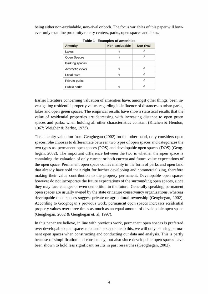
4

being either non-excludable, non-rival or both. The focus variables of this paper will how-

ever only examine proximity to city centers, parks, open spaces and lakes.

Table 1 –Examples of amenities

Amenity Non-excludable Non-rival

Lakes √ √

Open Spaces √ √

Parking spaces

Aesthetic views √ √

Local buzz √ √

Private parks √

Public parks √ √

Earlier literature concerning valuation of amenities have, amongst other things, been in-

vestigating residential property values regarding its influence of distances to urban parks,

lakes and open green spaces. The empirical results have shown statistical results that the

value of residential properties are decreasing with increasing distance to open green

spaces and parks, when holding all other characteristics constant (Kitchen & Hendon,

1967; Weigher & Zerbst, 1973).

The amenity valuation from Geoghegan (2002) on the other hand, only considers open

spaces. She chooses to differentiate between two types of open spaces and categorizes the

two types as: permanent open spaces (POS) and developable open spaces (DOS) (Geog-

hegan, 2002). The important difference between the two is whether the open space is

containing the valuation of only current or both current and future value expectations of

the open space. Permanent open space comes mainly in the form of parks and open land

that already have sold their right for further developing and commercializing, therefore

making their value contribution to the property permanent. Developable open spaces

however do not incorporate the future expectations of the surrounding open spaces, since

they may face changes or even demolition in the future. Generally speaking, permanent

open spaces are usually owned by the state or nature conservancy organizations, whereas

developable open spaces suggest private or agricultural ownership (Geoghegan, 2002).

According to Geoghegan’s previous work, permanent open spaces increases residential

property values over three times as much as an equal amount of developable open space

(Geoghegan, 2002 & Geoghegan et. al, 1997).

In this paper we believe, in line with previous work, permanent open spaces is preferred

over developable open spaces to consumers and due to this, we will only be using perma-

nent open spaces when constructing and conducting our data and analysis. This is partly

because of simplification and consistency, but also since developable open spaces have

been shown to hold less significant results in past researches (Geoghegan, 2002).

5

2.4 Environmental urban externalities

In the early work of Von Thünen (1826) he developed an economic theory called the

monocentric city model. In the model Von Thünen discusses a flat homogeneous land-

scape with one central business district (CBD), which is the main employer of the region.

Outside the city centers different sorts of agricultural goods are being produced and a bid-

rent relationship was developed suggesting that rent costs diminish with distance to the

CBD. Hence, it is increasingly more expensive to locate close to the CBD and increas-

ingly less expensive as one moves further away from the CBD. Yang and Fujita (1983)

developed a model to see the effect amenities implies on the location decision among

different income groups. Their main findings suggest that high income families tend to

locate outside the city centers, regardless of the amenities provided by the CBD.

Bruckner et al. (1999) did a similar research as Yang and Fujita (1983) they did however

extend this analysis and found that amenities do matter. They discovered that when ex-

ogenous amenities, such as parks, view of the water or historical monuments are located

in the city center they have the ability to attract high-income groups. Hence, their conclu-

sion is that if the amenity values of the city center are higher than in the suburbs the high

income people will locate in the center.

We may thus assume that, according to Bruckner et al. (1999) that amenities attract high

income earners. Thereby arguing that higher housing prices are expected when located

near an exogenous amenity. We also believe that the rent (housing prices) diminishes as

we move further away from the city center, as stated by Thünen (1826).

3 Models

3.1 Hedonic pricing

The hedonic pricing model act as the main pillar for this paper and will be the main guide

to explaining the value of amenities represented in the price of houses. The model works

as an intuitive analytical tool for examining the relationship between a good’s price and

its attributes. The theoretical foundation for hedonic pricing was provided by Lancaster

(1966) and was further developed by Sherwin Rosen in 1974, as previously mentioned in

section two. Despite the broad history and usage of the model, it still remains debated and

new research boundaries of the model are actively being pushed forward (Milon, 1984 &

Malpezzi, 2002). Hedonic pricing is a method that utilizes regressions to explain the

impact of different characteristics on the final price of a certain commodity. The hedonic

price model is traditionally expressed as a relationship between a dependent variable,

usually the price, and a set of independent variables that describes the existing variation

of goods in the market. There have been many empirical studies where the hedonic pric-

ing model has been used to investigate the price of a good. The equation of the model

may take on different forms but the most frequently used one is:

6

𝑃 = 𝑓(𝑧1, 𝑧2, … , 𝑧𝑛) (1)

Where P is the price of a specific good, in this case it will be the price of specific houses.

(z1, z2…... zn ) are different characteristics that one believes affect the housing prices.

As a simple example, a pair of jeans will distinguish itself from its competitors by having

a differentiated style, fabric, colour or some other characteristics that in the end will de-

termine the price of the pair of jeans in question. The use of the hedonic price model is to

determine the amount of the final price that can be accredited to each of these attributes

that makes the commodity unique. In this paper however, instead of jeans, we will apply

the hedonic price model on the housing market in Jönköping municipality.

Hedonic pricing has been extensively utilized for the purpose of analysing house prices

since the price determining characteristics are easily distinguishable (Tyrväinen, 1997).

Such characteristics in terms of the housing market involve three sub-groups, consisting

of the property itself, the environment and the location. The characteristics belonging to

the property itself are interpreted as internal characteristics while the location and envi-

ronmental attributes are considered to be external characteristics. Consequently, the he-

donic pricing method can be used as a way of obtaining the valuation of a house that is

solely accredited by external or internal factors respectively.

The hedonic price model has reached a high level of popularity since it is an easy and

straight-forward method for analyzing what fraction of the final house price can be ac-

credited to amenities such as distance to green spaces, lakes or parks. In other words, the

hedonic price model answers the following question: As there are no markets where ac-

tors can trade distances to natural amenities or city centers, how do we know the value of

these externalities?

The housing market is a very convenient market to use the hedonic pricing model, since

the commodity being sold holds easily distinguishable internal and external characteris-

tics that determines its final price. This is shown by the fact that consumers explicitly

express their preference of environmental and neighbourhood quality by purchasing a

house with low amounts of crime or close distance to water, parks and city centers in the

residential area. The extra premium paid for a house with no crime, compared to an iden-

tical house in an area with a higher crime rate, can be interpreted as the specific consumer

valuation of the neighbourhood quality.

3.2 Limitations of Hedonic Pricing

A successful model is used to portrait a simplification of the reality with as few assump-

tions as possible. However, in order to simplify the actuality there will always arise some

limitations that need to be addressed.

7

The first limitation of the hedonic price model is the probability of omitting vari-

ables. As an economist, it is very unlikely to be able to capture all of the good’s

characteristics that are reflected in its price, which may cause biased outputs of

the implicit price of the observed characteristics. The biasedness comes from the

chance of the omitted characteristics being correlated with the present character-

istics.

The second problem is regarding the possibility of the explanatory variables being

multiple correlated. For example, it is highly probable that large houses located in

rural areas also have increased proximity to open green spaces as well as lower

levels of air and noise pollution. Small houses however, are more frequently found

in urban areas, where open green spaces and parks are scarcer, accompanied by a

higher levels of both air and noise pollution.

The third limitation raises concern regarding information, or lack thereof. The

hedonic pricing model requires that each buyer has the ability to acknowledge

both the potential negative and positive consequences that may arise with the pur-

chase of a house. These externalities may include close distances to open green

spaces, water or parks or less displayed negative amenities such as pollution. Nev-

ertheless, in reality this previous knowledge and complete information is seldom

the case, especially if the externalities are negative.

Lastly, in order for the model to be as accurate as possible, large data is required

to support it, resulting in poor estimates when dealing with smaller amounts of

data.

4 Data

The data we will use to conduct our regressions and analysis originates from Pia Nilsson’s

doctoral work in the paper Price Formation in Real Estate Markets (Nilsson, 2013). The

data contains detailed information from the Municipal Housing and Development Office

regarding transactions of single family home purchases in Jönköping municipality during

the time period 2000-2011. The data also includes open space amenities such as open

green spaces, parks, forest areas and farmlands which is also provided by The Municipal

Housing and Development Office. We also want to include natural amenities such as the

proximity to water and open space amenities. This data is provided by the Swedish Me-

teorological and Hydrological Institute, The Swedish Environmental Protection Agency

and The Swedish Board of Agriculture (Nilsson, 2013).

The data includes over 8300 single family house purchases during a time span of 10 years,

stretching from 2000 to 2011, providing us with a sufficiently large dataset to conduct the

hedonic price regressions without being worried about poor estimates.

8

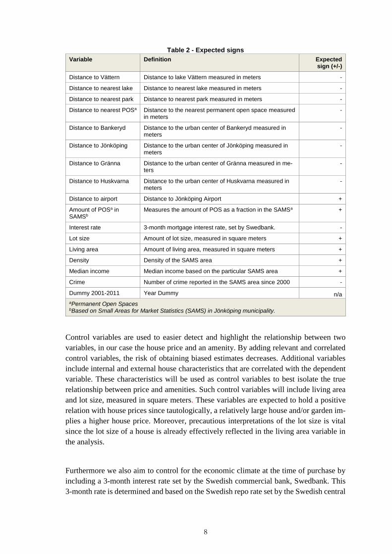
Table 2 - Expected signs

Variable Definition Expected sign (+/-)

Distance to Vättern Distance to lake Vättern measured in meters -

Distance to nearest lake Distance to nearest lake measured in meters -

Distance to nearest park Distance to nearest park measured in meters -

Distance to nearest POSa Distance to the nearest permanent open space measured in meters

-

Distance to Bankeryd Distance to the urban center of Bankeryd measured in meters

-

Distance to Jönköping Distance to the urban center of Jönköping measured in meters

-

Distance to Gränna Distance to the urban center of Gränna measured in me-ters

-

Distance to Huskvarna Distance to the urban center of Huskvarna measured in meters

-

Distance to airport Distance to Jönköping Airport +

Amount of POSa in SAMSb

Measures the amount of POS as a fraction in the SAMSa +

Interest rate 3-month mortgage interest rate, set by Swedbank. -

Lot size Amount of lot size, measured in square meters +

Living area Amount of living area, measured in square meters +

Density Density of the SAMS area +

Median income Median income based on the particular SAMS area +

Crime Number of crime reported in the SAMS area since 2000 -

Dummy 2001-2011 Year Dummy n/a

aPermanent Open Spaces bBased on Small Areas for Market Statistics (SAMS) in Jönköping municipality.

Control variables are used to easier detect and highlight the relationship between two

variables, in our case the house price and an amenity. By adding relevant and correlated

control variables, the risk of obtaining biased estimates decreases. Additional variables

include internal and external house characteristics that are correlated with the dependent

variable. These characteristics will be used as control variables to best isolate the true

relationship between price and amenities. Such control variables will include living area

and lot size, measured in square meters. These variables are expected to hold a positive

relation with house prices since tautologically, a relatively large house and/or garden im-

plies a higher house price. Moreover, precautious interpretations of the lot size is vital

since the lot size of a house is already effectively reflected in the living area variable in

the analysis.

Furthermore we also aim to control for the economic climate at the time of purchase by

including a 3-month interest rate set by the Swedish commercial bank, Swedbank. This

3-month rate is determined and based on the Swedish repo rate set by the Swedish central

9

bank, making them highly correlated, although the mortgage rate portraits the housing

market more accurately. The Swedish repo rate has been continuously declining for sev-

eral years and in April 2015 it hit a record low of -0.25% in order to deal with low inflation

and consumption levels (Riksbank, 2015). The interest rate is the main indicator of the

real estate market’s price levels since a lower interest rate suggests an increase in people’s

affordability when taking on mortgages. By lowering interest rate and making mortgages

more affordable, the demand for residential property increases and as a result so does the

price level. Since the 3-month mortgage rate is highly correlated with the repo rate, we

therefore expect a negative correlation between the house prices and this variable.

We also control for earning differences within the neighbourhood, sorted according to

Small Areas for Market Statistics (SAMS) regions, by including a median income varia-

ble. We expect neighbourhoods with a high median income to be willing to pay more for

a house, as well as being able to pay an extra premium to cluster with other high income

earners.

Furthermore, we also want to test for the distance to Central Business Districts (CBD),

since we assume CBD’s to be the main employers of the region (Alonso 1964; Mills 1972;

Muth 1969). As CBD’s we chose to include Jönköping as the largest employer and as

descending city centers we include the distance to the neighbouring cities of Bankeryd,

Gränna and Huskvarna. These distances highlight the importance of the geographical lo-

cation of a house and displays whether there is a strong negative correlation with increas-

ing distances to the CBD. The point location used for measuring the distances to urban

centers are the train stations in each town, since all of these are located in central areas

and are recognized as a good measurement of centrality. In order to gather the distances,

we apply the Pythagoras theorem using the SWEREF99 TM coordinates between the two

variables. The SWEREF99 TM calculates the specific location by measuring the amount

of meters north of the equator (initial value of 0) as well as the amount of meters east

from the central meridian, increasing eastwards (Lantmäteriet). The following formula

was used to calculate distance:

√((𝐂𝐎𝐑. 𝐘 − 𝐂𝐎𝐑𝟐. 𝐘)𝟐) + ((𝐂𝐎𝐑. 𝐗 − 𝐂𝐎𝐑𝟐. 𝐗)𝟐)

Where COR and COR2 corresponds to the different coordinates between the two points

between which the distance is being calculated. Since the distances we are measuring are

no extreme distances, we do not stress precaution about the surface of a sphere and there-

fore assume a 2D Euclidean plane. However, if the distances are being calculated at very

large scales, the distances along the surface are more curved and Pythagoras theorem does

not project correct distances. The same method of distance calculations was applied in all

cases where the distance was measured, including the proximity to water, open spaces

and airports.

10

The dummy variables included in the regression supports the isolation of the change in

house prices affected by that particular year and economic climate, compared to the year

2000. We chose to include 11 dummies ranging from a dummy for year 2001 all the way

to 2011. We are therefore excluding the year 2000 dummy since we treat this as the base

year and by including a dummy for each and every year creates perfect collinearity with

the intercept, avoiding the dummy variable trap.

In table 3, we highlight descriptive statistics to provide simple summaries to enable the

entrance of figures for comparability reasons. The descriptive statistics include the ex-

plaining variable as well as the explanatory variables. From the descriptive table we can

observe that there are more deviations in distance to the lake Vättern compared to the

distance to second nearest lake, this is intuitive and logical since the position of lake Vät-

tern is constant at one point on the geographical map and there is more than just one lake

in the municipality. Moreover the standard deviation of the amount of permanent open

spaces in the different SAMS areas is 2.63, indicating that there is a large difference be-

tween the SAMS areas when it comes to open spaces.

Table 3 - Descriptive Statistics

VARIABLES Mean Min Max Std. Deviation

Pricea 13.97 11.51 15.92 .76

Distance to Vättern 7.81 -.76 10.44 1.23

Distance to nearest lake 7.96 1.85 9.31 .78

Distance to nearest park 6.40 2.20 9.73 .91

Distance to nearest POS 6.86 1.54 8.38 .88

Distance to Bankeryd 9.24 4.68 10.57 .88

Distance to Jönköping 8.81 6.09 10.65 .80

Distance to Gränna 10.25 4.59 11.09 .69

Distance to Huskvarna 8.90 5.37 10.61 .88

Distance to airport 9.16 6.84 10.78 .60

Amount of POS in SAMS -4.52 -11.04 -.21 2.63

Lot size 6.74 4.38 10.50 .74

Living area 5.17 3.40 6.82 .34

Density 1.82 -3.55 4.23 1.64

Median income -1.02 -1.60 -.47 .22

Crime 1.27 -3.69 3.67 1.37

Interest rate 2.40 .42 4.00 1.28

aDependent variable

All variables presented in logged form.

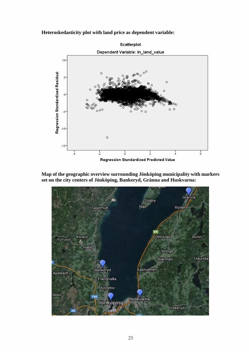
Furthermore, in the appendix we include a map with markers set on the city centers of

Jönköping, Bankeryd, Gränna and Huskvarna in order to give some geographic overview

to the readers without any prior knowledge about the geographical area surrounding Jön-

köping.

11

4.1 Functional form

Linear, semi-logged and double logged functional forms have all been heavily used and

examined in previous literature (Rosen, 1974; Freeman, 1974; Nilsson 2013; Tyrväinen,

1997; Milon 1984) and they all contain weaknesses that limit the use of data and the

interpretation of the results. For the purpose of this paper, we will be conducting the he-

donic regressions in double-log form. We are using a double-logged functional form be-

cause there are diminishing returns to the dependent variable as well as most of the ex-

plaining characteristics determining the dependent variable.

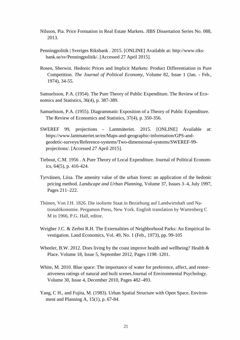
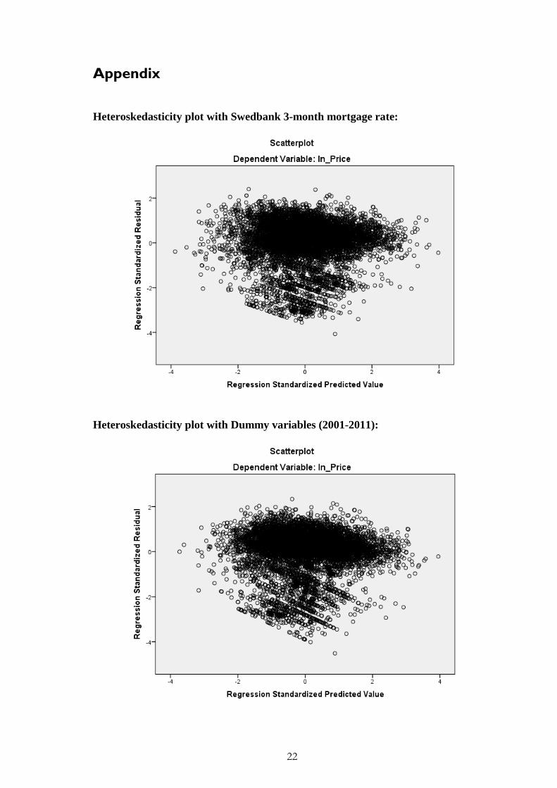
A problem that might occur by not using a semi-log or double-log form is the risk of

obtaining heteroskedasticity. Heteroskedasticity occurs when the error terms in the re-

gression do not have constant variance and are in some way systematically dependent on

some explanatory variable (Goodman, 1995). For example, if the errors of house prices

increase as the living area increases, we may be exposed to heteroskedasticity. Scatter-

plots displaying the degree of heteroskedasticity is included in the appendix.

The hedonic price model applied in this paper takes the following form:

ln 𝑃𝑟𝑖𝑐𝑒𝑖 = 𝛽1 + 𝛽2ln𝐷. 𝑉Ä𝑇𝑇𝐸𝑅𝑁𝑖 + 𝛽3ln𝐷. 𝐿𝐴𝐾𝐸𝑖 + 𝛽4ln 𝐷. 𝑃𝐴𝑅𝐾𝑖 +𝛽5 ln𝐷. 𝑃𝑂𝑆𝑖 + 𝛽6 ln 𝐷. 𝐵𝑁𝐾𝑅𝑌𝐷𝑖 + 𝛽7 ln 𝐷. 𝐽𝐾𝑃𝐺𝑖 + 𝛽8 ln 𝐷. 𝐺𝑅Ä𝑁𝑁𝐴𝑖 +𝛽9 ln 𝐷. 𝐻𝑆𝐾𝑉𝑅𝑁𝑖 + 𝛽10 ln 𝐷. 𝐴𝐼𝑅𝑃𝑂𝑅𝑇𝑖 + 𝛽11 ln 𝐴𝑀𝑂𝑈𝑁𝑇. 𝑃𝑂𝑆𝑖 +𝛽12ln𝐿𝑂𝑇. 𝑆𝐼𝑍𝐸𝑖 + 𝛽13ln𝐿𝐼𝑉. 𝐴𝑅𝐸𝐴𝑖 + 𝛽14ln 𝐷𝐸𝑁𝑆𝐼𝑇𝑌𝑖 + 𝛽15 ln INCOME𝑖 + 𝛽16 ln 𝐶𝑅𝐼𝑀𝐸𝑖 + 𝛽17 𝐼𝑁𝑇𝐸𝑅𝐸𝑆𝑇. 𝑅𝐴𝑇𝐸𝑖 + 𝜀𝑖

Where ln 𝑋 is the natural logarithm of variable X , 𝛽1 is the intercept, D refers to distance

and 𝜀𝑖 is an error term.

5 Data results and analysis

In this part of the paper, we will discuss and analyze the outputs from the regressions

regarding house prices in Jönköping. We begin by analyzing the fit of the model and our

focus variables before examining our control variables.

Below the variables in Table 4, we find an R-squared for each specific regression model.

By observing the R-squared we find that there is a decline from 0.327 in model 1 to 0.212

in model 2. This can be interpreted as the goodness of fit for the model and that the inde-

pendent variables are explaining 32.7% and 21.2% of the variation in the housing prices.

Generally, this might seem like a low R-squared. However, as mentioned in section 3.2

the most common limitation of the hedonic regression approach is the risk of omitting

variables. By omitting variables, the R-squared will drop due to less explanatory power

of the variables. This occurs due to the house characteristics being preferred differently

by different individuals, which in turn makes it unmanageable to capture all of these as-

pects within a single model. We also lack the data regarding all internal and external

house characteristics since the costs of obtaining such immense data would be extremely

expensive and time consuming.

12

Table 4 - Regressions

MODEL 1

t

MODEL 2

t VARIABLES β β

(Constant) 11.971** 20.126 13.093** 20.405

Distance to Vättern -.117** -9.520 -.104** -7.885

Distance to nearest lake -.021* -1.909 -.024** -1.964

Distance to nearest park -.020** -2.037 -.014 -1.344

Distance to nearest POS .016 1.627 .017 1.599

Distance to Bankeryd -.238** -6.023 -.238** -5.572

Distance to Jönköping -.152** -7.038 -.151** -6.475

Distance to Gränna -.100** -5.391 -.111** -5.534

Distance to Huskvarna -.050** -3.911 -.045** -3.265

Distance to airport -.116** -4.245 -.091** -3.090

Amount of POS in SAMS .041** 9.664 .035** 7.689

Lot size .055** 4.269 .035** 2.514

Living area .549** 22.869 .536** 20.676

Density .013* 1.794 .013* 1.761

Median income -.175** -3.686 -.044 -.866

Crime -.053** -5.219 -.033** -3.005

Interest ratea - - -.111** -18.920

Dummy 2011 1.009** 27.204

Dummy 2010 .775** 21.518

Dummy 2009 .702** 19.545

Dummy 2008 .590** 16.580

Dummy 2007 .569** 15.984

Dummy 2006 .447** 12.478

Dummy 2005 .203** 5.750

Dummy 2004 .263** 6.920

Dummy 2003 .213** 5.449

Dummy 2002 .115** 2.976

Dummy 2001 .040 1.032

R 0.572 0.461

R-squared .327 0.212

Observations 8318 8318 a3-month mortgage rate set by Swedbank Dependent Variable: Price **. Significant at the 0.05 level. *. Significant at the 0.1 level

5.1 Focus variables

The focus variables of this paper are the distance-based amenity variables, including dis-

tance to city centers, permanent open spaces and other natural amenities. We predicted

that as distance to these variables increases the price of the house will decrease, suggest-

ing a negative relationship. Based on our regression, our hypothesis was proven to be true

for all except for one amenity variable. The distance to Vättern, the nearest lake and the

distance to nearest park all hold this negative relationship with housing prices which we

predicted in the section 4, the same holds for the distances to city centers. This is in line

13

with the economic theory of Buchanan (1965), Tiebout (1956), Bruckner et al. (1999)

Von Thünen (1826) all of which, with different approaches, state that housing prices will

be higher when the house is located near one of these amenities.

Being the second biggest lake in Sweden and the sixth in Europe, Vättern holds an impact

of decreasing house prices of 0.117% according to model 1 and 0.104% according to

model two, when increasing the distance to Vättern by 1%. Due to the location of Jönkö-

ping city and the U-curved shape of the southern part of lake Vättern, this distance vari-

able might be captured in other variables such as the distance to the Jönköping variable.

Moreover, due to the extensive length of the Vättern’s southern coast line, the different

house price levels represented along this region are exposed to significant volatility.

We also wanted to examine how much of an impact the distance to the closest lake and

park has on house prices. The result from these variables are as expected, but with mixed

significance. Proximity to nearest lake has a decreasing impact of more than 0.02% of the

price if the distance to the lake increases by 1%, with a significance level of 10% for

model 1 and 5% for model 2. The park-proximity variable holds a similar relationship

with house prices and we can observe that we get a negative and statistically significant

value of 0.020 for model 1 and a negative value without any significance of 0.014 for

model 2. This implies, according to model 1, that the house price will drop slightly with

0.02% as we increase the distance to the nearest park by 1%.

Distance to permanent open spaces (POS) is however positively related with distance to

the observed houses, but not to a significant level. This is the contrary to our expectations

and thus deviates from the result of the work by (Geoghegan, 2002 & Geoghegan et. al,

1997) where she states that a neighbourhood consisting of a large fraction of permanent

open spaces will face an increase in property values. However, a positive relationship

may be explained by the definition of what permanent open space amenities are. Since

we have distance to parks and lakes as separate variables, the distance to nearest POS-

variable may include less attractive open spaces such as swamp marks, farm lands and

other government protected environmental areas that may not be very desirable. The dis-

tance to the nearest POS-variable therefore absorbs more of the open spaces that does not

increase the value of the property. This is shown by the positive but not significant coef-

ficient values of 0.016 for model 1 and 0.017 for model 2.

As additional focus amenities, we chose to include distances to city centers. For the pur-

pose of this paper, we have chosen to include Jönköping, Huskvarna, Bankeryd and

Gränna as city centers as they capture complete or parts of the definition of a CBD (Thü-

nen, 1966). The cities are all negatively correlated with property prices and this is in line

with our prediction regarding distances to the nearest urban centers. This is explained

theoretically in the monocentric city model where the bid-rent curve suggest that the rent

is higher near the central business district. In this case, it might be up for debate to define

some of our city centers of choice as being central business districts. However, in order

14

to prove a point, this definition is assumed to hold for all city centers and thus is part of

the explanation for the negative relation with house prices and distances to CBD’s.

Furthermore, close distance to the cities of Jönköping, Huskvarna, Bankeryd and Gränna

do all absorb other city amenities than being the main employer. Such city amenities are

restaurants, bars, shopping, local buzz and other leisure amenities. The results from our

regression models all held true to our expectations of the signs and all four of the distances

between property and city centers show a negative relation with house prices at a 5%

significance level. The most prominent city-distance variable is surprisingly the distance

to Bankeryd. This variable shows a coefficient value of -0.238 where both regression

models support the negative relationship argued above, and may be interpreted as a de-

crease in the house price of 0.238% alongside an increase in the distance between Bank-

eryd and the property by 1%. As Jönköping is the biggest city center amongst these vari-

ables, we expected this variable to have more impact on prices as it plays a crucial role

as main employer of the region. Contrarily, the distance to Jönköping city was the second

most influential city-distance variable and presented that with a 1% increase in distance,

we observed a decrease of the house price equivalent to more than 0.15%. The other two

city-distance variables of Gränna and Huskvarna are both also statistically significant at

a 5% level but have a lower impact on house prices. The reaction of increasing the dis-

tances to Gränna and Huskvarna by 1% are equivalent to a price reduction of 0.1% and

0.05%, respectively, according to model 1.

The reasoning behind Bankeryd being the most prominent city-distance variable instead

of Jönköping is unclear to us since we expected Jönköping to have the biggest impact due

to the comparably higher supply of positive externalities being created in the bigger city

of Jönköping. However, according to Yang and Fujita (1983) high income families may

tend to locate outside the city centers regardless of the amenities and externalities sup-

plied by the city center, and this might provide one reasoning of why the Bankeryd vari-

able contributes the highest effect on house prices.

5.2 Control variables

In Table 4, regression model 1 includes dummy variables for each year beginning in 2001

and ending in year 2011. These dummies provide a clear indication of the development

of the prices on the housing market in Jönköping municipality. All values are significant

at a 5% significance level except for the Dummy 2001 variable, meaning that there was

not enough changes in housing prices between the year 2000 and 2001. The property

prices tend to increase each year according to the estimates, except for the years 2001 and

2005. In 2007 and 2008 house prices experienced minor stagnation due to the recession

during these years. If we observe the development of the dummy coefficients over time,

there is a very clear increasing trend that corresponds to the overall trend observed in real

house prices in Sweden over these specific years. The last year of our observation shows

that the prices had risen about 100% in nominal terms since 2000, which is a fair estimate

in accordance to the report by Statistics Sweden which states that the overall development

15

of house prices in Sweden increased by 196% in nominal terms since 1990 (Statistics

Sweden).

When obtaining the results from regressions containing both the dummy variables and

the mortgage rate, we noticed that either our mortgage rate variable or the Dummy 2009

variable got excluded from the regression output. This was due to the variables being too

correlated with each other, with a negative Pearson correlation of over 0.5, as shown in

Table 5. Our interpretation of this is that the overall trend of the dummy variables are so

closely correlated with the 3-month mortgage rate that one of the two has to be excluded.

The highest correlation occurred between the interest rate and the dummy for 2009 and

that is why that particular dummy got excluded. In order to deal with this issue, we de-

cided to split the regression in two different models, one including the dummy variables

to control for change over time and excluding the mortgage rate, and the reverse for model

2.

Table 5 – Pearson Correlation

Dummy 2009 Interest rate

Dummy 2009 1 -.505**

Interest rate -.505** 1

**. Correlation is significant at the 0.01 level (2-tailed).

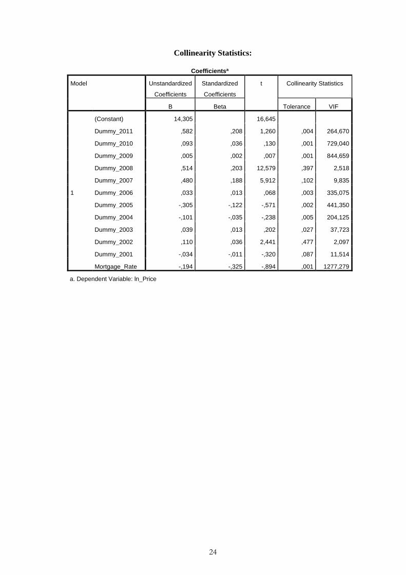
Furthermore, we checked for multicollinearity between the interest rate and the dummy

variables by observing the Variance Inflation Factor (VIF). The VIF values for the

dummy variables were all high and for the interest rate variable we observe a very high

value of 1277.279, indicating that there indeed are multicollinearity between the varia-

bles. The VIF values are all included in the appendix.

In regression model 2, where the mortgage rate is included, we find a negative relation

between the interest rate and house prices as hypothesized in section 4. The mortgage rate

variable is linear compared to most of the other variables included in the regressions that

are logged. This will lead to a different, log-linear interpretation of the variable. The co-

efficient value of -0.111 is significant at a 5% significance level, suggesting that an in-

crease in the 3-month mortgage rate of 1% will lead to a decrease in house prices by

11.1%. The 3-month mortgage rate set by Swedbank is by far the most dominant factor

that contributes to changes in prices. Since investing in a house may be the biggest in-

vestment of your life, this is an obvious key factor when purchasing a house.

The outcomes from the regression regarding internal house characteristics are in line with

our expectations. In both regression models, the lot size and living area are positively

correlated with the house price at a 5% significance level. The amount of square meters

are one of the most influential factor on house price and this can be shown by observing

the beta coefficients of 0.549 and 0.536, suggesting that a one percent increase in the

living area, measured in square meters, will affect the final house price by more than

16

0.5%. The lot size however does not have nearly the same impact on house prices as the

living area. By observing the house transactions where we find the largest lot sizes, we

also find that they are most often located on the outskirts of the municipality. According

to Von Thünen (1826), this relation is due to falling prices as we increase the distance

from urban centers, and this is why the lot size variable is not heavily affecting the house

price. The impact of the lot size in model 1 indicates that a 1% increase in the lot size will

increase the house price by 0.055% and in the second regression model this value has

dropped to a price increase of 0.035%. The values of the coefficient are significant at a

5% level for both models.

The density variable measures the density of the population living in a particular SAM’s

area. We expected a positive correlation of this characteristic to the house prices and this

turned out to hold true according to our regressions. However, the impact of a dense area

does not give an impressive impact on the house prices in Jönköping. The beta value for

the density is only 0.013, stating that a slight increase of one percent of the SAMS-area

density will produce a 0.013% increase in the price. The density variable is significant

for both regression models, but only at a 10% level. Our conclusion is that the density of

a particular SAM’s area contains people that owns single family homes but also people

that resides in other forms of living, such as rentals and apartments. This will lead the

density variable to not fully capture the effect of only single family home purchases since

everybody in the SAMS area are included in the variable. The higher density does there-

fore not necessarily mean that the demand for houses is greater where the density is larger.

Which may be the explanation of a fairly low value of the coefficients.

As neighbourhood variables we have included the median income and crime rate in the

specific SAMS areas. When looking at the median income variable, it deviates from our

expected direction. As can be observed in Table 4, the sign for both models are negative

suggesting a lower price as the median income increases in a particular SAM’s area. The

coefficient is however only significant in regression model 1. The reasoning and interpre-

tation behind this is unclear, since rational thinking suggest that an area where the median

income is high, we would expect that the demand for expensive houses would be higher

as well. The outcome from the crime variables are suggesting significantly lower prices

as the percentage of crimes increase in the area. For regression model 1, an increase of

1% in crime leads to a decrease in house prices of 0.053% and for model 2, the suggested

price decrease is 0.033% if the crime rate would increase by 1%.

5.2.1 Land value and focus variables

The results from the conducted regression models 1 and 2 displayed the falling house

price relationship with our focus variables as predicted, however they did not display the

relation as clear as expected. It was therefore decided to run a regression with the valua-

tion of the land that each house was built upon as the dependent variable. We conducted

this robustness test to merely control for the impact of distances to our focus variables

and thereby allow the exclusion of all characteristics and attributes surrounding the house.

17

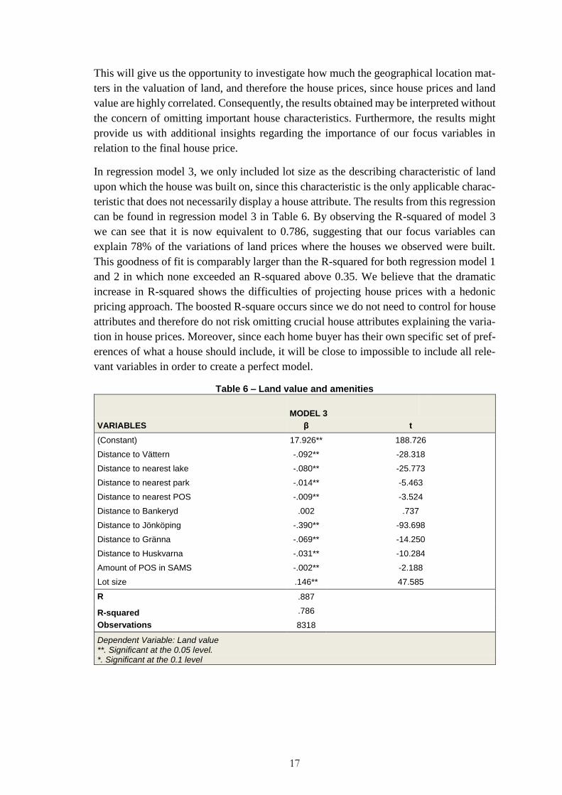
This will give us the opportunity to investigate how much the geographical location mat-

ters in the valuation of land, and therefore the house prices, since house prices and land

value are highly correlated. Consequently, the results obtained may be interpreted without

the concern of omitting important house characteristics. Furthermore, the results might

provide us with additional insights regarding the importance of our focus variables in

relation to the final house price.

In regression model 3, we only included lot size as the describing characteristic of land

upon which the house was built on, since this characteristic is the only applicable charac-

teristic that does not necessarily display a house attribute. The results from this regression

can be found in regression model 3 in Table 6. By observing the R-squared of model 3

we can see that it is now equivalent to 0.786, suggesting that our focus variables can

explain 78% of the variations of land prices where the houses we observed were built.

This goodness of fit is comparably larger than the R-squared for both regression model 1

and 2 in which none exceeded an R-squared above 0.35. We believe that the dramatic

increase in R-squared shows the difficulties of projecting house prices with a hedonic

pricing approach. The boosted R-square occurs since we do not need to control for house

attributes and therefore do not risk omitting crucial house attributes explaining the varia-

tion in house prices. Moreover, since each home buyer has their own specific set of pref-

erences of what a house should include, it will be close to impossible to include all rele-

vant variables in order to create a perfect model.

Table 6 – Land value and amenities

MODEL 3

VARIABLES β t

(Constant) 17.926** 188.726

Distance to Vättern -.092** -28.318

Distance to nearest lake -.080** -25.773

Distance to nearest park -.014** -5.463

Distance to nearest POS -.009** -3.524

Distance to Bankeryd .002 .737

Distance to Jönköping -.390** -93.698

Distance to Gränna -.069** -14.250

Distance to Huskvarna -.031** -10.284

Amount of POS in SAMS -.002** -2.188

Lot size .146** 47.585

R .887

R-squared .786

Observations 8318

Dependent Variable: Land value **. Significant at the 0.05 level. *. Significant at the 0.1 level

18

The most prominent change can be observed in the relation between land price and the

distance to Jönköping city center. This coefficient, according to the regression in Table

6, is now -0.390 which implies that a 1 % increase in distance to Jönköping city decreases

the price of the land by -0,390 %. This is more than twice as much as in the regressions

in Table 4 where the coefficients are -0.152 in model 1 and -0.151 for model 2 respec-

tively. Our interpretation of this is, when filtering out all internal house characteristics

and only focusing on location, Jönköping city center is the most essential. As previously

discussed, this might be due to the higher amount of externalities and amenities Jönköping

city provides. The municipality of Jönköping holds a somewhat homogenous landscape,

suggesting that distances to natural amenities such as water or parks might not play a

crucial role since they are fairly distributed over space. Therefore we conclude that the

coefficient boost in proximity to Jönköping is based on urban amenities and externalities

provided by the city center, beyond the distance to natural amenity variables. This is also

the results from regression model 3 where we see that the distance to lake Vättern only

decreases the price of the land by 0.092% if the distance to Vättern increases by 1%,

significant at a 5% level. Moreover, the distance variables to the nearest lake and park

only displays a significant negative relationship of 0.08 for lakes and 0.14 for parks, sug-

gesting a very small change in land prices when increasing the distances from them. An-

other big deviation between the first two regression models and the regression conducted

in Table 6 is the significance of the distance to Bankeryd. From being the most prominent

distance-to-city-center variable in Table 4 to being a non-significant variable when ex-

cluding all house attributes in regression model 3. This result gives us the reason to doubt

our previous reasoning that high income families tend to locate outside the city centers,

as mentioned in section 5.2.

6 Conclusion

In this paper we studied the relationship between single family home prices and the dis-

tance to natural amenities such as lakes, parks and open spaces. This relationship was also

tested for the distance to city centers since it captures urban amenities and being the main

employer. This was done by using a dataset containing information regarding single fam-

ily home purchases in Jönköping, Sweden during the years 2000 and 2011. The valuation

of the amenities are based on a hedonic pricing approach stating that the house consists

of a bundle of utility bearing characteristics that are subjectively valued. By running re-

gressions according to this model we, as a result, observed and identified the extent to

which the fraction of the price is accredited to these specific amenities.

The main findings in the study are that there indeed exists a negative relation with in-

creasing distances between the focus variables and house prices. Although the signifi-

cance levels of the distance to natural amenity variables do not hold constant over the

different regression models, they do however still present a correlated, yet slightly

skewed, negative relationship. Beside the natural amenities, we tested what effect the

distance to urban centers have on house prices. In Jönköping municipality we chose to

19

include Jönköping, Bankeryd, Huskvarna and Gränna as urban centers since they all pos-

sess properties of being a CBD according to the definition by Von Thünen (1826). The

outcomes of these variables, observable in Table 4, do overall hold a greater impact on

the house prices compared to the natural amenities. Additional research is necessary to

investigate what specific factors within the city centers contribute to increased house

prices in this geographical study area.

Furthemore, we computed a robustness test by substituting the dependent variable to the

land value of the houses, instead of the house price itself, in order to filter out the dif-

ficulties of projecting house prices with a hedonic pricing approach. This erased the pos-

sibility of omitting crucial house characteristics that explains the variation in the depend-

ent vairable. Moreover, since there is a correlation between the price of a house and the

corresponding land value, we where able to explain that geographical location matters

without using internal house characteristics in the regression model. The result presented

in regression model 3 in Table 4 shows that people value to be located in proximity to

Jönköping city center more than the other city centers. Further we see that natural ame-

neties are attractive and that proximity to water is the most prominent coefficents among

the natural ameneties.

Our two main regression models, 1 and 2 in Table 4, obtained an R-squared of 0.327 and

0.212 respectively, compared to a coefficient of determination of 0.787 in model 3. It is

therefore suggested that future research investigates how to obtain the optimal functional

form that is able to better explain the variations in the dependent variable.

20

References

Alonso W. Location and Land Use. Toward a general theory of land rate. 1964. Cam-

bridge: Harvard University Press. 1964

Bourassa, Steven C, Hoesli, Martin E., Sun, Jian. 2003. What's in a View?

Brueckner J.K. Why is central Paris rich and downtown Detroit poor?: An amenity-based

theory. European Economic Review. Volume 43, Issue 1, January 1999, Pages 91–

107.

Buchanan, J.M. (1965). An Economic Theory of Clubs. Economica, 32(125), p. 1- 14.

Freeman, A.M. (1979). Hedonic Prices, Property Values and Measuring Environmental

Benefits: A Survey of the Issues . The Scandinavian Journal of Economics, 81(2),

p. 154-173.

Geoghegan J. (2002). The value of open spaces in residential land use. Land use policy,

Vol. 19(1), 91-98.

Geoghegan et. al, 1997. Spatial landscape indices in a hedonic framework: an ecological

economics analysis using GIS. Ecological Economics, 23 (3) (1997), pp. 251–264

Goodman, A.C, 1997. Dwelling-Age-Related Heteroskedasticity in Hedonic House Price

Equations: An Extension. Journal of Housing Research, Vol. 8 Issue 2.

Kitchen W. & Hendon S. Land Values Adjacent to an Urban Neighborhood Park. Land

Economics, Vol. 43, No. 3 (Aug., 1967), pp. 357-360

Lancaster, Kelvin J. A New Approach to Consumer Theory. The Journal of Political

Economy, Vol. 74, No. 2 (Apr., 1966), 132-157.

Malpezzi, Stephen. 2002. Hedonic Pricing Models: A Selective and Applied Review.

Housing Economics and Public Policy. Blackwell Science Ltd, Oxford, UK, 2002.

Mendelsohn, R. & Olmstead, S. 2009. The Economic Valuation of Environmental

Amenities and Disamenities: Methods and Applications. Annu. Rev. Environ. Re-

sour. 2009. 34:325–47

Milon, JW. 1984. Hedonic Amenity Valuation and Functional Form Specification. Land

Economics Vol. 60, No. 4 (Nov., 1984), pp. 378-387

Mitchell, R. 2009. Effect of exposure to natural environment on health inequalities: an

observational population study. The Lancet 372 (9650), 1655-1660.

21

Nilsson, Pia. Price Formation in Real Estate Markets. JIBS Dissertation Series No. 088,

2013.

Penningpolitik | Sveriges Riksbank . 2015. [ONLINE] Available at: http://www.riks-

bank.se/sv/Penningpolitik/. [Accessed 27 April 2015].

Rosen, Sherwin. Hedonic Prices and Implicit Markets: Product Differentiation in Pure

Competition. The Journal of Political Economy, Volume 82, Issue 1 (Jan. - Feb.,

1974), 34-55.

Samuelsson, P.A. (1954). The Pure Theory of Public Expenditure. The Review of Eco-

nomics and Statistics, 36(4), p. 387-389.

Samuelsson, P.A. (1955). Diagrammatic Exposition of a Theory of Public Expenditure.

The Review of Economics and Statistics, 37(4), p. 350-356.

SWEREF 99, projections - Lantmäteriet. 2015. [ONLINE] Available at:

https://www.lantmateriet.se/en/Maps-and-geographic-information/GPS-and-

geodetic-surveys/Reference-systems/Two-dimensional-systems/SWEREF-99-

projections/. [Accessed 27 April 2015].

Tiebout, C.M. 1956 . A Pure Theory of Local Expenditure. Journal of Political Econom-

ics, 64(5), p. 416-424.

Tyrväinen, Liisa. The amenity value of the urban forest: an application of the hedonic

pricing method. Landscape and Urban Planning, Volume 37, Issues 3–4, July 1997,

Pages 211–222.

Thünen, Von J.H. 1826. Die isolierte Staat in Beziehung auf Landwirtshaft und Na-

tionalökonomie. Pergamon Press, New York. English translation by Wartenberg C

M in 1966, P.G. Hall, editor.

Weigher J.C. & Zerbst R.H. The Externalities of Neighborhood Parks: An Empirical In-

vestigation. Land Economics, Vol. 49, No. 1 (Feb., 1973), pp. 99-105

Wheeler, B.W. 2012. Does living by the coast improve health and wellbeing? Health &

Place. Volume 18, Issue 5, September 2012, Pages 1198–1201.

White, M. 2010. Blue space: The importance of water for preference, affect, and restor-

ativeness ratings of natural and built scenes.Journal of Environmental Psychology.

Volume 30, Issue 4, December 2010, Pages 482–493.

Yang, C H., and Fujita, M. (1983). Urban Spatial Structure with Open Space. Environ-

ment and Planning A, 15(1), p. 67-84.

22

Appendix

Heteroskedasticity plot with Swedbank 3-month mortgage rate:

Heteroskedasticity plot with Dummy variables (2001-2011):

23

Heteroskedasticity plot with land price as dependent variable:

Map of the geographic overview surrounding Jönköping municipality with markers

set on the city centers of Jönköping, Bankeryd, Gränna and Huskvarna:

24

Collinearity Statistics:

Coefficientsa

Model Unstandardized

Coefficients

Standardized

Coefficients

t Collinearity Statistics

B Beta Tolerance VIF

1

(Constant) 14,305 16,645

Dummy_2011 ,582 ,208 1,260 ,004 264,670

Dummy_2010 ,093 ,036 ,130 ,001 729,040

Dummy_2009 ,005 ,002 ,007 ,001 844,659

Dummy_2008 ,514 ,203 12,579 ,397 2,518

Dummy_2007 ,480 ,188 5,912 ,102 9,835

Dummy_2006 ,033 ,013 ,068 ,003 335,075

Dummy_2005 -,305 -,122 -,571 ,002 441,350

Dummy_2004 -,101 -,035 -,238 ,005 204,125

Dummy_2003 ,039 ,013 ,202 ,027 37,723

Dummy_2002 ,110 ,036 2,441 ,477 2,097

Dummy_2001 -,034 -,011 -,320 ,087 11,514

Mortgage_Rate -,194 -,325 -,894 ,001 1277,279

a. Dependent Variable: ln_Price