Embed Size (px)
Citation preview

Valuation of a Spark Spread:
an LM6000 Power Plant
Mark Cassano∗
Gordon Sick†
September 6, 2011
Abstract
This paper analyzes a power plant powered by two General Electric LM6000 gasturbines combined with a steam generator that allows combined cycle operations.We consider four distinct operating modes for the plant.
Such a plant can be characterized as a real option on a spark spread: optimallyconverting natural gas to electricity. We use a Margrabe approach by using themarket heat rate (the ratio of the electricity price to the natural gas price) as ourunderlying stochastic variable.
We estimate a stochastic model for market heat rates that incorporates time ofday, day of week, month and the incidence or otherwise of a spike in heat rates.We use the model and its residuals in a bootstrap process simulating future marketheat rates, and use a Least Squares Monte Carlo approach to determine the optimaloperating policy.
We find that the annual average market heat rate is a good explanatory variablefor the time-integral of the plant operating margin, denominated in the naturalgas numeraire. This allows us to express plant values in terms of the numeraireand convert to dollars by multiplying this by the natural gas forward curve and aforward curve of riskless discount rates.
We also provide information about the optimal operating modes selected, thenumber of transitions between modes, and how they relate to transition costs andthe average heat rate for the year.
∗Consultant, Calgary†Haskayne School of Business, University of Calgary

1 Introduction
This paper analyzes a power plant in Alberta, Canada, that is powered by two General
Electric LM6000 gas turbines combined with a steam generator that allows combined
cycle operations. The LM6000 is derived from the engine GE supplies for Boeing 767
and 747 airplanes. It is adapted for natural gas by General Electric. This power plant is
popular in various power jurisdictions around the world as a turnkey power plant that
can offer peaking capacity, and some baseload power delivery.
We consider 4 operating modes for the plant: cold metal (off), 15 MW idle in com-
bined cycle, full simple-cycle power (95 MW) and combined cycle full power (120 MW).
It is common to refer to such a plant as generating a spark spread: converting natural
gas to electricity by burning. A spark spread has two correlated stochastic variables:
electricity price and natural gas price. To lower the dimensionality of the problem, we
work with heat rates. The market heat rate is the ratio of the electricity price to the
natural gas price and the plant heat rate is the number of gigajoules (GJ) of gas needed
to generate one MWh of electric power. This allows us to analyze the problem using the
Margrabe approach, using natural gas as the numeraire commodity.
We estimate a stochastic model for market heat rates that incorporates time of day,
day of week, month and the incidence or otherwise of a spike in heat rates. We use the
model and its residuals in a bootstrap process simulating future market heat rates, and
use a Least Squares Monte Carlo approach to determine the optimal operating policy.
We find that the annual average market heat rate is a good explanatory variable
for the time-integral of the plant operating margin, denominated in the natural gas
numeraire. This allows us to express plant values in terms of the numeraire and convert
to dollars by multiplying this by the natural gas forward curve and a forward curve of
riskless discount rates.
1

2 Option Valuation Based on the Market Heat Rate
The value of a natural gas based power plant centers on the difference between the prices
of electricity and gas (often termed the spark spread); in fact, one can look at a gas
powerplant as being a call option on the spark spread (a “spread option”). The operator
of the plant has the option to convert a given number of gigajoules (GJ) of natural
gas, at the plant’s operational heat rate, into a number of megawatt-hours (MWh) of
electricity. Being able to generate power strategically is a significant source of value and
the value of this flexibility can be found by applying modern financial derivative pricing
techniques. Since the power plant converts gas to electricity, the “unit of account” for
the exchange is GJ of natural gas. This contrasts with the typical way of regarding
options, which is the right to exchange a quantity of dollars for a unit of the underlying
asset. Commonly, a call option on a stock is the right to buy the underlying stock for a
fixed number of dollars. In contrast, a spread call option on a stock gives the holder a
right to buy a share of stock for a fixed number (e.g. say 2) shares of another stock.
Margrabe (1978) was the first to study the option to exchange one asset for another.
He only considered European options, but made the seminal observation that it was
useful to model the ratio of the prices of the two underlying assets, so that one asset is
priced relative to the other as a numeraire. This reduces the two-dimensional problem
to one dimension. Martzoukos (2001) extended the exchange option to the option to
exchange one of several risky assets for a particular risky asset (perhaps a risky strike
price), taking the latter asset as the numeraire asset. Kulatilaka (1993) applied the
exchange option notion to a real option context for switching between fuels for a boiler.
Deng et al. (2001) valued a gas-fired generator as a strip of European call options on
the ratio of the electricity price to the gas price. Their model has no switching cost to
turn the generator on and off, so the decisions are simple and not a sequence of related
decisions. Gardner and Zhuang (2000) model a gas-fired generation asset with a constant
2

fuel cost, but mean reverting electricity prices and switching cost by a lattice approach.
Carmona and Durrleman (2003) employed the Margrabe model to value generators as
spark spreads. Nasakkala and Fleten (2005) model the spark spread (with a fixed plant
heat rate) as the sum of a mean-reverting Ornstein-Uhlenbeck process and an arithmetic
Brownian motion and estimate the joint spot and forward prices with a Kalman filter
model. In Fleten and Nasakkala (2010), they allow the plant to ramp up or down, with
no direct switching costs. They use this to determine plant value and assess investment
and abandonment options. Hlouskova et al. (2005) model a spark spread for a plant that
has a quadratic heat rate in output, switching costs and ramp-up and ramp-down times.
3 Seasonality and Price Spikes in the Electricity Market
Natural gas and electricty markets have seasonality and electricity markets also have
price spikes.
Elliott et al. (2002) model electricity price spikes with a regime-switching model,
where the regimes are defined by the number of baseload generators that are oper-
ating in the power pool. There is a discrete Markov hourly process for the number
of baseload generators running. Within each regime, electricity prices follow a mean-
reverting diffusion, so the price spikes (up and down) occur at the times of the regime
switches. Kamat and Oren (2002) model electricity prices with a mean-reverting affine
jump diffusion and obtain closed-form valuation for a variety of exotic European op-
tions. Carmona and Durrleman (2003) review a variety of computational techniques
for the value of European spread options on two stochastic underlying assets, including
analytic approximations and simulation. The underlying stochastic processes can follow
arithmetic or geometric Brownian motion, and have Poisson-distributed jumps. Huis-
man and Mahieu (2003) model jumps in electricity prices with a regime-switching model
where there are three regimes. Goto and Karolyi (2004) study the US, Nord Pool and
3

Australian markets with a mean-reverting conditionally autoregressive heteroskedastic-
ity (ARCH) model with time-varying (seasonal) Poisson jumps. Mount et al. (2006)
develop a regime-switching model of electricity prices in the PJM market. There are
two regimes: a spike and non-spike regime. Seifert and Uhrig-Homburg (2007) compare
Poisson spike and regime-switching jump models for daily price jumps and spikes in the
German electricity market. Kanamura and Ohashi (2007) develop a structural model
of electricity prices in the PJM market in which the supply curve follows a Box-Cox
transformation that generalizes the exponential function. They compare this to a jump
diffusion model with Poisson jumps. Howison and Coulon (2009) have an equilibrium
electricity price model of supply bids (merit order stack) and stochastic demand. They
model the New England Pool (NEPool) with gas prices affecting supply and the PJM
pool with gas prices and coal prices affecting supply. This leads to power spikes, as
generators with higher cost are bid into the system. Heydari and Siddiqui (2010) model
the log of gas and electricity prices jointly with annual and weekly sinusoidal seasonality,
and mean reversion. They model electricity spikes with a regime-switching model (two
regimes) and stochastic volatility.They use this process to value a gas-fired power plant
that has no switching costs.
4 Electricity and Natural Gas Prices in Alberta
In Alberta, there is “postage-stamp pricing” for electricity and natural gas. That is,
the wholesale price of natural gas, in dollars per gigajoule ($/GJ), is set on a daily
basis (often called the AECO or NIT price) in a competitive market, and the same price
prevails for all delivery points in Alberta. The wholesale price of electricity, in dollars per
megawatt-hour ($/MWh), is set on an hourly basis (often called the System Marginal
Price or SMP) in a competitive market, but the same price prevails throughout Alberta.
Alberta has an abundant supply of natural gas and coal. Most electric power is
4

generated by large, efficient baseload coal-fired plants, which are not very flexible in
their operations. They yield a relatively inelastic supply of electricity. Alberta is in the
rainfall shadow of the Rocky Mountains, so there is very little hydro power available.
This is a problem, since hydro power is a major source of price-responsive peaking power.
The only other major source of peaking power is a gas-fired turbine, such as the GE
LM6000 that we study in this paper.
Let SEi (in $/MWh) and SGi (in $/GJ) be the electricity and gas prices, respectively,
for observation hour i. The market heat rate is defined as the ratio of the two, Yi :=
SEi /SGi (measured in GJ/MWh). It is the natural-gas value of electricity; specifically,
how many GJ of natural gas to acquire one MWh of electricity. If the acquisition is done
in the market, it is a market heat rate. As an example, assume the gas price is $6.25/GJ
and electricity is $40/MWh. The market heat rate would be 40/6.25 = 6.40 GJ/MWh.
We also have a plant heat rate. It is also the number of GJ of natural gas that is
needed to produce one MW of power. In this case, the acquisition is done by burning
the natural gas in the plant to produce electricity. Continuing our example above, a
power plant that has an operational heat rate greater than 6.40 GJ would be “out of
the money” — the amount gas required to generate a MWh is more than the quantity
of gas that a MWh of electricity is worth in the market. A power plant that is inflexible
may not be able to be turned off economically when the plant is out of the money.
For modeling and valuation, we define the natural logarithm of the market heat rate
as yi := ln(Yi) = ln(SEi /SGi ).
Figures 1 and 2 show the time series and distribution of historical hourly heat rates
(respectively) in the Alberta market for the years 2002-2006. The central feature of the
graphs, and the source of the option-like value of the power plant, are the spikes. These
spikes typically do not last for a long time, as their causes (such as weather or generator
outages) are usually temporary. In addition, at high heat rates, supply responds, as less
efficient generation becomes economical. The majority of heat rates are below 20, but
5

Figure 1: Historical Alberta hourly market heat rate: 2002-2006. This figure overstatesthe magnitude of the heat rates because the pixel width covers several hours. If a spikeoccurs beside a low heat rate, the low heat rate is hidden by the spike adjacent to it,so we only see the high heat rate. However, there is clear evidence of spikes in the heatrates.
6

0%
5%
10%
15%
20%
25%
30%
35%
40%
45%
0 5 10 15 20 25 30 35 40 45 50 55 60 65 70 75 80 85 90 95 100
Freq
uency
Hourly Market Heat Rate (GJ/MWh)
Figure 2: Histogram of Alberta hourly market heat rate (GJ/MWh): 2002-2006. Thehorizontal axis labels give the upper limit of the bin for each value in the histogram
7

Table 1: Summary statistics of the market heat rate Y , log of heat rate y = lnY andthe hourly changes in y. The units for Y are GJ/MWh and the units for the hourly rateof change ∆y are basis points (0.01%).
Year Mean Y Std Y Mean y Std y Mean ∆y Std ∆y2002 11.5830 17.7420 2.1013 0.7690 -0.21173 48952003 10.0830 11.1920 1.9660 0.8165 -1.50471 60642004 8.7909 8.4864 1.8766 0.7945 0.11283 61832005 8.2296 8.9049 1.7418 0.8685 1.39150 62532006 14.0070 23.4530 2.1460 0.8682 0.04920 5359Overall 10.5380 15.2490 1.9663 0.8374 -0.02430 5777
there is positive skewness from a significant number of spikes (e.g. heat rates greater
than 20).
Table 1 presents the averages and standard deviations for the market heat rate (Y )
and the log of the market heat rate (y) for the years 2002 to 2006. As one can see, there
is a “U” shape to the average heat rates; 2006 having the highest average heat rates, and
2004 and 2005 having the lowest market heat rates. The table also provides statistics
for the hourly change in y, which is the hourly rate of change in Y , and the units are in
basis points (1 basis point = 0.01%). The mean rate of change is close to zero because
the prices revert to the mean in the long run, with little systematic growth or decline.
But, the standard deviation of the hourly rate of change is in the range of 49%–63%.
This is quite high, largely because of the price spikes. This volatility is rather constant
over the years, but it does have a slight inverted “U” shape, which is opposite to the
effect for the market heat rate. Thus, in years when heat rates are low, the volatility is
generally somewhat higher, consistent with a leverage effect.
As we will discuss in Section 6, the spikes make standard deviations harder to inter-
pret. For example, the 2002 heat rates have the second largest standard deviation but
the lowest log standard deviation.
Figure 3 shows the distribution of the hourly rate of change (in basis points) of the
Alberta market heat for 2002–2006. Almost 25% of the changes are between -1% and
8

0%
5%
10%
15%
20%
25%
30%
-‐10,00
0
-‐9,000
-‐8,000
-‐7,000
-‐6,000
-‐5,000
-‐4,000
-‐3,000
-‐2,000
-‐1,000
0
1,000
2,000
3,000
4,000
5,000
6,000
7,000
8,000
9,000
10,000
100,000
Freq
uency
Range of Hourly Rate of Change of Market Heat Rate (basis points)
Figure 3: Histogram of hourly rate of change of the Alberta market heat rate (basispoints): 2002-2006. The horizontal axis labels give the upper limit of the bin for eachvalue in the histogram
9

0% and a further 13% are between 0% and 1%, so the market heat rate usually changes
very little from hour to hour. But 5% of the time, there was a negative spike with a
price drop of over 100%1 and 5.1% of the time, there was a positive spike with a price
increase of over 100%.2
5 Valuation Issues
5.1 The Margrabe Approach
The Margrabe approach is useful for valuing spread or exchange payoffs, where a good
of uncertain value is exchanged or converted into another good of uncertain value. To
understand the Margrabe approach, we first discuss a more common situation of capital
budgeting for a foreign investment.
The discussion above has everything denoted in Canadian dollars (CAD). If the cash
flows are in British Pounds (£), we must multiply all Pound values by appropriate
exchange rates and also discount at the Canadian interest rate, in order to compute
a value in CAD. For example, if the Pound cash flow (CF£) is in 2 years, we’d could
convert this future Pound cash flow into CAD at the 2 year forward exchange rate, and
then discount at the Canadian risk free interest rate. If FT is the two year forward rate
(in CAD per £) and rCAD is the Canadian interest rate, the PV in CAD is CF£×FT ×
e−rCADT . Alternatively, we could arrive at a Pound PV by discounting the Pound cash
flow at the British interest rate and then convert it to CAD at the current (spot) exchange
rate (call it S£). The PV in CAD would be CF£×e−rUKT×S£. Both approaches arrive at
the same answer because the interest rate parity arbitrage in foreign exchange markets
implies FT = S£e(rCAD−rUK)T . To summarize, the two ways to compute PV in CAD
when the future cash flow is in British Pounds are:1Since these are changes in the logarithm, a change of -10,000 basis points or -100% does not send
the price to zero, but represents a price reduction of exp(−1)− 1 = −63% over one hour.2Again, since these are logs of prices, the 100% figure in the table is a price increase of exp(1)− 1 =
172%.
10

• Use the T year forward exchange rate (CAD per £) and discount using the Cana-
dian interest rate.
• Use the spot exchange rate (CAD per £) and discount using the British interest
rate.
Thus, there is nothing inherently special about currencies such as the British Pound.
In fact, the key to our Margrabe valuation approach is putting values in terms of natural
gas rather than British pounds or Canadian dollars. The future “cash flow” is in GJ of
natural gas. Substituting “£” with GJ of natural gas we have the two ways of converting
the future value in GJ of gas to the PV in CAD of our power plant:
• Use the T year forward or futures price of natural gas (CAD per GJ) and discount
using the Canadian interest rate.
• Use the spot price of gas (CAD per GJ) and discount using the natural gas “interest
rate” from a forward or swap curve.
In our case, the first method is more practical. Suppose the future gross margin is vT GJ
of gas for a plant that is operated optimally over the year T to T + 1. Hence the PV in
CAD is V0 = e−rTFTE∗0[vT ] where FT is the CAD forward price for natural gas, set at
time 0 for delivery at time T .
5.2 The Certainty-Equivalent Method
Options and derivatives analysts value assets by incorporating risk in the expectation
of the cash flow in the numerator of the PV formula. This risk-adjusted expectation is
a certainty-equivalent (CE). The CE is discounted at the riskless discount rate in what
is called risk-neutral valuation. Suppose the market heat rate payoff is f(yT ). The risk-
neutral valuation is PV = e−rTE∗[f(yT )] where E∗[f(yT )] is the expected payoff after
the distribution of market heat rates has been changed to incorporate risk.
11

We assume that risk-neutral expectations of the market heat rate are equivalent
to actual expectations. That is, we assume the market risk premium for electricity is
approximately equal to that of gas, so that the risk premia cancel each other in the
exchange option.
To see how this works, consider a standard option on a single non-traded asset (or
one that has a return below the market rate). McDonald and Siegel (1984) and Sick
(1989, 1995) show how we can impute a dividend from the Capital Asset Pricing Model,
as in the Black and Scholes (1973) alternative CAPM derivation of the partial differential
equation for option pricing. If an asset is priced in equilibrium by the CAPM then
α+ δ = rf + β(Em − rf )
or
rf − δ = α− β(Em − rf )
where
α = actual drift rate of the underlying risk
δ = dividend yield on the underlying asset, imputed from CAPM equilibrium
rf = riskless rate of return
β(Em − rf ) = CAPM risk premium on the underlying asset
This provides two alternative ways of characterizing the risk-neutral growth rate of
the underlying asset rf − δ = α − β(Em − rf ). We use the second approach based on
the risk premium, which has also been proposed in a general equilibrium setting in (Cox
et al., 1985, Lemma 4). Extending this to the Margrabe model, the risk-neutral growth
12

rate to consider is the logarithm of the heat rate (the ratio of the electricity price to the
gas price), which is the difference of the logarithms. Thus, the risk-neutral growth rate
of the heat rate is
αE − βE(Em − rf )− (αG − βG(Em − rf ))
= αE − αG − (βE − βG)(Em − rf )
where αE , αG, βE , βG are the growth rates and betas of electricity and gas, respectively.
(Martzoukos, 2001, Equation 3) uses a similar result in which the risk-neutral drift
rate for a Margrabe option in a multivariate geometric Brownian motion setting is the
difference between the drift rates of the two risky assets. He couches this in terms of the
convenience yields δ of the assets, but given the CAPM equivalence above, it generalizes
to the definition of the risk-neutral drift as the actual drift minus a CAPM risk premium.
Since electricity is priced in the long run off of the gas price curve in many markets
such as Alberta, we assume that they have the same systematic risk (βE = βG), and the
risk premium term drops out. Thus, the growth rate of the heat rate in the Margrabe
model can be taken to be the same as the growth rate of risk-neutral growth rate. This
means we do not have to introduce a risk-premium into our simulation model to correctly
price the spark spread options.
6 Modeling and Estimation of the Market Heat Rate
While there is a long-term futures market for natural gas, there is not for electricity, so
we can’t use information from the term structure of forward prices to assist in estimating
a model of the spot heat rate. Thus, we just examine the historical behavior of the spot
market heat rate. The data set we used consisted of hourly Alberta Price pool electricity
prices and daily Alberta AECO gas prices from 2002 to 2006.
The most common models used for valuation are based on Brownian motion for
13

the logarithm of the underlying asset prices, which makes the underlying processes log-
normally distributed. The spikes present in electricity prices (and the relevant market
heat rates) require a more complicated model; the empirical distributions do not come
close to resembling a normal or log-normal distribution. We use a regime switching model
where the underlying price switching randomly between two or more different processes.
One regime is “normal” and the other regime is a “spike” regime that could occur due
to a demand or supply shock such as abnormal weather or a base load generator outage.
Each hour, the market heat rate is in one of the two regimes and behaves according to
the stochastic rules of the given regime. We also need a stochastic model for the regime
switching process. Hence we must estimate the following:
• The stochastic characteristics of the “normal” regime - we’ll name the normal
regime Regime 1.
• The stochastic characteristics of the “spike” regime - we’ll name the spike regime
Regime 2.
• The “switching” process which is the nature of how likely we are to switch from
one regime to another.
We define the spike regime as occurring when the market heat rate is greater than 20
(i.e. Y > 20 or y > ln(20) = 2.996).We considered other spike definitions, but this led
to simulations that best resembled the actual historical behavior. For each of Regime
j = 1, 2, we use linear regression to estimate the following equations:
yi = βj (hour of day,day of week,month of year, year) + γjyi−1 + εi,j (1)
The estimation is done with dummy variables so there are no regression coefficients for
Hour 1, Sunday, January, or the Year 2002. The lagged observation, yi−1 captures tem-
porary non-regime-switching shocks. It also eliminates serial correlation in the regression
14

residuals, εj . This is an important quality when using these residuals for bootstrapping
in the Monte Carlo study.
We estimate the probability of being in each regime with a logistic regression. Define
the binary variable Ri = 1 if a spike occurs at hour i and Ri = 0 otherwise. Then use a
logistic regression to find the best fit minimizing the least squares distance between the
observed Ri and the logistic function R where R = ezi/(1 + ezi) and
zi = βr (hour of day,day of week,month of year, year) + ψRi−1 . (2)
Logistic regression is a numerical way of estimating the probability of each regime in
the data observed; for example, if spikes occur more in October, Ri will be more likely
to be a 1 and the logistic regression coefficient for an October dummy variable will be
positive and significant.3
The results of our analysis are given in Table 2.
6.1 Example using the estimation results
As an example of how to use Table 2, assume it is Hour 11 (HE 11) on a Wednesday
in October 2007 and the current market heat rate is 8. Note that ln(8) = 2.0794.
Since 8 < 20, we are in Regime 1. If we use the stylized year 2002 (to reflect the
average annual heat rates and spike probability), to determine the expected value of the
log market heat rate in the next hour (Hour 12), we add the appropriate coefficients
to the constant term. For example, the expected log market heat rate for regime 13The Margrabe approach uses a geometric Brownian motion for the ratio of the two prices. In our
model, the heat rate ratio will be geometric Brownian motion within each regime, but will jump at eachregime switching point. Thus, it is not a continuous geometric Brownian motion for the whole period.That would present a problem in the European option situations that Margrabe considered, because heused the Black-Scholes model to value the European option to exchange one asset for another. We useLeast Squares Monte Carlo (LSM) techniques to analyze the sequence of American options to switchamongst operating modes. The LSM approach does not require geometric Brownian motion. Thus, wedo not have a strict Margrabe model in our paper, but we continue to use the term in deference to thenotion of modeling the ratio of two prices as a univariate stochastic process, rather than the two pricesas two separate jointly distributed prices.
15

Table 2: Estimated regime and regime-switching probability models. For the regimemodels, the dependent variable is the log heat rate and the lag variable is the previouslog heat rate. The logistic regression estimates the probability of a spike and the laggedvariable is a dummy variable that is one only if the previous regime was the spike regime.All other independent variables, are dummy variables that are 1 only if the describedtime condition occurs.
Variable Regime 1 Regime 2 Logistic Regression
Constant 0.3685 2.6246 -4.6182Hour 2 0.1679 0.0000 0.0000Hour 3 0.0845 0.0000 -0.5733Hour 4 0.0806 0.0000 -0.8620Hour 5 0.1342 0.0000 -0.9841Hour 6 0.2608 0.0000 0.0000Hour 7 0.4362 0.2554 1.4019Hour 8 0.2578 0.0000 0.6749Hour 9 0.5941 0.0000 1.2641Hour 10 0.5478 0.0000 1.2453Hour 11 0.5640 0.1074 1.6926Hour 12 0.5097 0.0000 1.7470Hour 13 0.4363 0.0000 1.2879Hour 14 0.4486 0.0984 1.6905Hour 15 0.4372 0.1103 1.5376Hour 16 0.4505 0.0843 1.6950Hour 17 0.5530 0.1437 2.2390Hour 18 0.4877 0.1267 2.1675Hour 19 0.3023 0.0000 1.1408Hour 20 0.4112 0.0000 1.6318Hour 21 0.4715 0.0000 1.4570Hour 22 0.4953 0.0000 1.7075Hour 23 0.0748 0.0000 0.0000Hour 24 0.3056 0.0000 1.6465
Mon 0.0728 0.0000 0.3061Tues 0.0701 0.0000 0.1144Wed 0.0694 0.0000 0.0000
Thurs 0.0830 0.0000 0.0000Fri 0.0970 0.0000 0.0000Sat 0.0422 0.0000 0.0000Feb -0.0238 0.0000 -0.4007Mar 0.0000 0.0000 0.0000Apr -0.0350 0.0000 -0.3650May -0.0212 0.0000 0.0000Jun -0.0557 0.0000 0.0000Jul 0.0221 0.0000 0.4321Aug 0.0522 0.0000 0.0000Sep 0.0264 0.0000 0.0000Oct 0.0377 0.1020 0.5759Nov 0.0551 0.0000 0.2553Dec -0.0618 0.0992 0.00002003 -0.0829 0.0000 0.26332004 -0.0829 -0.0647 -0.16572005 -0.1488 -0.0796 0.00002006 -0.0424 0.1339 0.5156Lag 0.5978 0.2984 2.6853
16

is .3685 + .5097 + .0377 + .5978 × ln(8) = 2.1591. Given that there is volatility, the
expected price is not e2.1591 = 8.66. If the heat rate was normally distributed, the
expected heat rate would be e2.1591+σ2/2 where σ is the standard deviation of the log
heat rate. Given that the historical standard deviations are approximately 0.8, this
would imply an approximate mean heat rate of e2.1591+.82/2 = 11.93. A similar exercise
for regime 2 has the expected log market heat rate being 3.3471 and the expected heat
rate being approximately 39.13.
Given that we are in regime 1, the probability of being in a spike regime in the next
hour (Hour 12) is determined by the logistic equation. Using the logistic regression, we
repeat a similar coefficient as above, arriving at a total of z = −4.6182+1.747+ .5759 =
−2.2953. This is converted to a probability using the logistic function ez/(1 + ez), hence
the probability of being in a spike regime is e−2.2953/(1+e−2.2953) = 9.51%. This implies
that the expected market heat rate would be equal to the expected heat rate across the
two regimes: 11.93× .905 + 39.13× .095 = 14.42.
If the market heat rate in Hour 11 was much higher we alter the previous analysis
by changing the lagged variable. For example if the market heat rate was 50 (where
ln(50) = 3.9120), we would expect log market heat rates of 3.2547 and 3.8940 for regimes
1 and 2, respectively. This gives approximate heat rates of 35.68 and 67.62 for the two
respective regimes. The likelihood of staying in regime 2 would be 59.63% implying an
expected heat rate of 54.73.
To show how the stylized year affects these results, assume the stylized year was 2006
(the “spikiest” year). The market heat rate of 8 results in expected log heat rates of
2.1167 and 3.481, and expected heat rates of 11.44 and 44.75, in the Regimes 1 and 2,
respectively. Also, there is a 14% chance of Regime 2 (spike) in the next hour. For a
market heat rate of 50, we find expected log heat rates of 3.2123 and 4.078 and expected
heat rates of 34.20 and 77.32 for the two regimes, with a 71% chance of continuing the
spike.
17

In Table 2, for the normal regime, we see that market heat rates tend to be highest
in the daytime and evening (hours 9 to 22). Weekdays tend to have higher heat rates
than weekends. Heat rates also tend to be higher in the summer and fall. These are
all consistent with the fact that the electricity price is in the numerator of the heat
rate. Also, heat rates tend to be sticky, with an auto-covariance of 0.5978, but there is
some mean reversion, since that coefficient isn’t 1. In the spike regime, these variables
have much less explanatory power. The main driver of the heat rate process in the
spike regime is the high constant, reflecting a high overall heat rate, and the lower
autocovariance term, suggesting stronger mean reversion. In the logistic regression, we
see that there is a much higher probability of a spike in the late afternoon (hours 17 and
18), and a generally high probability of a spike in the day and evening. There is a higher
spike probability in July, October and November. This may be because these months
are used for planned maintenance of power plants, and some of the large baseload plants
tend to be offline then. Finally, the high lag coefficient in the logistic regression suggests
that spikes are somewhat persistent, although that coefficient of 2.6853 is smaller in
magnitude than the constant of -4.6182, indicating that spikes do tend to go away.
7 Monte Carlo Simulations
Simulation has been used by Calistrate et al. (1999) and Alesii (2005) to assess the
risk-management properties of a real options strategies, but neither used it to form
conditional expectations, valuation and optimization of the real options strategy.
For valuation, we extend the simulation technique to the Least Squares Monte Carlo
(LSM) method (see, for example Broadie and Glasserman (1997); Longstaff and Schwartz
(2001); Glasserman (2003)). In addition, Alesii (2008) studied the convergence properties
of the LSM method in univariate and multivariate settings, finding it to be very useful in
multivariate settings (where other techniques are slow), but not converging very quickly
18
if the underlying stochastic processes were not mean reverting.
The LSM approach is a clever combination of a simulation (running forward in time)
with dynamic programming optimization (moving backward in time). The essential
idea can be understood by thinking how the lattice (“binomial”) approach (see, e.g.
Cox et al. (1979)) works to value an American call option, while also determining the
optimal exercise policy. The lattice approach provides risk-neutral probabilities at each
point in a lattice or tree for the tree nodes that could be achieved one step later. This
allows the computation of the risk-neutral expected value of the various policy decisions
(exercise the option or not, in the case of a call option) that can be made at each node.
Using the Bellman approach, the highest-valued policy is taken and this optimal value is
carried back to the earlier time period, allowing the optimization to proceed backward
in time. The important observation is that the binomial method allows the computation
of risk-neutral expectations of next-period value for each decision policy.
The LSM approach proceeds in a similar way, but calculates the risk-neutral expected
values of the policies by regressing actual next-period values in the simulation on known
state variables at each decision point (the operating mode and the value of the stochastic
state variables and deterministic variables — time and seasonal variables). The optimal
exercise decision policy is the one that gives the highest value for each set of known
state variables. Initially, a simulation of all the stochastic state variables provides a
set of simulated paths for the state variables. One time step before the last date, the
final-period values generated by each possible policy decision are regressed onto the
information that would be known at the earlier time step. This allows the computation
of conditional expectations of the value of each policy one step before the end. The
optimal values are recorded and used as payoffs for a regression using information at the
time two steps before the final date. This gives conditional expectations, and the whole
process is repeated to give a sequence of regression coefficients for each date and for each
policy decision that can be made at that date. Decisions can be made by comparing the
19

conditional expected values of the policies and choosing the most valuable decision.
In our application, the values of the various policy decisions consist of the one-period
present value of the expected next-period value (of the optimally operated plant) minus
the value of any switching costs needed to change operating modes. In our situation,
the switching costs are the inferior plant heat rate that arises during transition periods.
That is, more fuel is burned, and not as much power is generated. We also consider a
model below in which a 1000 GJ penalty is added to each transition, in order to reduce
the number of transitions in the model.
While the decisions are path dependent, a sufficient statistic for the path history is
to know a vector consisting of the current operating mode of the plant, as well as the
values of the stochastic processes at that date. Thus, the path dependency creates no
problems in this analysis because the vector stochastic processes are Markovian and the
information needed to describe the operating state has a low dimension.
Our LSM method relies on simulating hourly heat rates of the power plants. One
often uses a pre-specified distribution such as normal or log-normal and matches the
distribution’s parameters to the data. However, for market heat rates, there is no obvious
distribution that adequately describes the salient features of the data.
To simulate heat rates, we bootstrap, using the residuals from the two regime regres-
sions, εi,j from equation (1) to generate the random characteristics of the market heat
rate. The specifics of a one-year simulation are as follows:
• An initial market heat rate, hour, day of week, month, and stylized year are spec-
ified. We used an initial market heat rate of 10, Hour 1, Monday, January for all
of the simulations.4
• The logistic regression is used to simulate the regime of the first hour (Hour 1).4The nature of the simulations (and the subsequent valuations) is not affected by the initial market
heat rate and day of week because the shocks and seasonality effects have a very short duration. Theinitial heat rate of 10 is a round number close to the long-run market heat rate of 10.538 reported inTable 1.
20

This is done by drawing a uniform random number (i.e. a random number between
0 and 1, which is the typical way a computer generates a random number) and
comparing this number with the probability of being in the spike regime which is
determined as described in Section 2. If the simulated uniform number is less than
the spike probability, then there will be a spike (i.e. hour 1 will be in regime 2).
If the uniform number is greater than the spike probability, then the regime will
be normal (i.e. regime 1).
• Once the regime is determined, the market heat rate comes from the expected log
price regression and drawing randomly from the residuals of the relevant regime
regression.
• This process is then repeated. The hour, day of week, month is adjusted appro-
priately; the new regime and heat rate are now used in the 3 estimated equations.
Figure 4 shows simulated runs using this bootstrapping method for 4 stylized years.
The 2004 simulations are similar. Comparing this figure with Figure 1, the random
nature of the simulated heat rates bear a strong resemblance to that of the historical
market heat rates. This is important for the option value of the power plants depend
crucially on the dynamic behavior of the market heat rate, the most important being
the spike levels and durations.
These figures were a single representative simulation for each year. We ran 100
simulations for each stylized year. Figure 5 shows the distribution of heat rates for
each year. We can see that 2006 has a higher average heat rate and a much more
dispersed distribution. This is due to the higher spike probability. The stylized year
2005 distribution is the most “bearish” distribution. When we perform our valuation
exercise, it is these 5 possible stylized years that we use.
21

Figure 4: Simulated market heat rates for four stylized years. The market heat rate isin GJ/MWh. The hours are measured starting at 1 am on January 1.
22

Figure 5: Distribution of heat rate from 100 simulations in each stylized year.
23

8 Modeling the Operating Characteristics
An earlier version of this paper was developed for a consulting client that wishes to
remain anonymous. We are grateful that they have permitted us to create a modified
form of the report as a research paper. To protect their proprietary interests, we have
modified the plant characteristics slightly with the effect that a precise valuation is not
possible. However, the broad issues in the analysis are still correct. We have not modified
the analysis in the previous sections, since they are based on publicly available data on
market prices, although we are grateful to the client for having gathered it for us.
We obtained operating performance characteristics from a visit to a power plant
owned by the client that had two LM6000 gas turbine generators and a steam generator
that could generate power from the heat of the turbine exhaust. We collected actual
operating data (heat rates and output capacity on a minute-by-minute basis) for a ramp
up and ramp down of one gas turbine in combined cycle mode. We understand that
the ramp up and ramp down can be done more rapidly than in our sample, and it is
often limited by the Power Pool System Operator, which does not like to have the plants
increasing or decreasing output more rapidly than 5 MW/minute because they need time
to adapt the system to the changes in generation. We modified the data to be consistent
with ramp up and ramp down at 5 MW/minute, while still allowing for pauses for heat
soak and other characteristics specific to the gas and steam turbines.
Our analysis only considered a restricted set of operating modes for the plant, which
were consistent with optimal heat rates for a given range of outputs. We analyzed
the plant as a merchant power plant that did not have any contract or obligation to
provide Ancillary Services, such as spinning reserve capacity, to the Power Pool. The
actual operating data had the plants running in intermediate modes that we did not
model. While these intermediate modes could represent suboptimal operating decisions,
it seemed more likely that the intermediate operating modes arose from one of the
24

following considerations:
• The plants could have been contracted to provide Ancillary Services. This would
generate revenue, and we did not collect data on this, nor did we examine the types
of Ancillary Services contracts that were available. The decision to contract for
Ancillary Services could generate more value than our merchant power model, but
we were not in a position to assess this. In particular, we were not in a position
to model future markets for Ancillary Services.
• Our visit to the plant led us to understand that the plant operators use more
data to make their decisions than we used in our model. In particular, they pay
attention to the whole supply schedule (“merit order”) and the demand schedule
for electricity in the system. In many cases the plant is running at a heat rate that
makes it the marginal supplier of power, so bidding in a second generator could
depress the system marginal price (SMP) so much that the first generator would
start losing money. Our model assumed a perfectly elastic demand curve, and that
no other power suppliers would adjust their production in response to changes by
our plant. In other words, we assumed a perfectly competitive electricity market.
But, when the plant is at the margin (its operating heat rate is the market heat
rate), optimal decisions by the plant operator should include consideration of the
effect on SMP and this can result in intermediate operating modes.
8.1 Plant Operating Modes
We considered 4 operating modes:
Cold Metal was the mode where no fuel was burned and no power was generated.
15 MW Idle Combined Cycle was the mode where 1 gas turbine was synchronized
and idling in combined cycle mode. In this mode, it burned fuel at 168 GJ/hour
25

for a heat rate of 11.2 GJ/MWh. This mode allowed a fairly rapid ramp-up to full
combined cycle output, but power produced in this idle mode is quite expensive,
compared to typical market heat rates.
Full power from two simple cycle gas turbines generated 95 MW of power with
a fuel burn of 931 GJ/hr and a heat rate of 9.8 GJ/MWh. The gas turbines ramp
up more quickly than the steam turbine, so this mode capture price spikes before
steam generation can start up.
120 MW Full Combined Cycle Output burned fuel at 938 GJ/hr for a heat rate
of 7.90.
We also considered all possible transitions amongst these four modes, using the per-
formance data from the plant visit. To ramp up steam production and enter combined
cycle mode required 4 hours from cold metal or a gas turbine mode. Ramp down took
0.483 hours to 1.4 hours, depending on the transition. The ramp up from the 15 MW
Idle Combined Cycle to full Combined Cycle output took 0.95 hours.
8.2 Sequential Ramp Up and Ramp Down
All of our transitions assumed that the operator would start up one gas turbine at a time.
This sequential operation allows the operator to study the generator closely, to check for
problems. In theory, it might be possible to start up two gas turbines in tandem, but
the System Controller would not like such a sudden surge of power anyway.
9 Least Squares Monte Carlo Valuation
In order to value a power plant with flexible operating characteristics, one must deter-
mine the optimal operating policy of the plant. Entering into a given hour, the plant
has a current operating mode. The manager uses all available information (hour, day
26

of week, month, and stylized year, as well as the current operating mode and market
heat rate) to determine whether to have the plant remain in the current mode or switch
to another mode. The manager must consider the cash flow for the next hour, plus the
remaining value of the plant, given the operating mode in which the manager’s decision
leaves the plant. For example, the manager may be tempted to capture a spike at 9
pm, just as Hour 22 starts. This is an hour with generally high cash flows and a high
probability of a spike, given the data in Table 2. The payoff could be lucrative for the
next hour, but turning on the generator at this time would leave it in operation in the
next hour, when value is likely to be low. Thus, the manager must consider not only the
cash flow for the next hour, but also the “residual value” of the state that the decision
gives the plant at the end of the hour. This residual value is the value of the cash flow
for the remainder of the year, given the decision.
Each decision implies a “switching cash flow”, which is the value (in GJ of natural
gas) of the electricity produced minus the amount of natural gas used during the switch,
given the plant heat rate. This also includes the fractional part of the hour (if there
is one) after the switch is completed. As an example, if the switch takes 40 minutes,
the switching cash flow is the electricity produced minus the natural gas used during
the 40 minutes of the switch plus the 20 minutes at which the plant is operating in the
new mode. When there is no switch, the “switching” cash flow is simply the value of
producing electricity at the current mode. The remaining value is the total value of
operations for the remainder of the year from the hour after the switch has been made,
given the mode into which the manager has put the plant and the market data on gas
prices and electricity prices. This is a dynamic programming problem, which is solved
recursively in the next subsection.
27

9.1 The Dynamic Programming Problem
Assume the plant operates for one year. The value of the plant in operational model m is
a function of the hour h of the year and the current market heat rate. We denote this as
Vh(m, yh). The solution method uses backward induction; we start at the final hour H in
the year, and determine the switching cash flows going from mode m to all other possible
modes. LetM be the set of operating modes and denote the switching cash flows of going
from mode m to m′ as πh(m,m′). The cash flow πh will also depend on the current and,
for transitions longer than an hour, expected future market heat rates. We suppress these
heat rate arguments to simplify this discussion. As mentioned, if we remain in the current
operating mode, the switching cash flow is the operating cash flow π(m,m) = yh − km.
For the final hour the value function is VH(m, yH) = maxm′∈M πh(m,m′). We need
the following notation; let τ(m,m′) be the hours of time required to transition from
operating mode m to m′.
Since our transition times are either less than one hour or equal to four hours, we
can find the value functions for the penultimate hour, H − 1 as follows. Given a current
operating mode m and market heat rate yH−1 the value of changing the operating mode
to m′ is
νH−1(m,m′, yH−1) =
E [πh(m,m′) + VH(m′, yH) | yH−1] : τ(m,m′) 6 1
E [πh(m,m′) | yH−1] : τ(m,m′) > 1(3)
Note than if m′ = m, the plant stays at the current operating mode. E [• | yH−1] is the
expected value operator conditional on information available at hour H − 1. The value
function in hour H − 1 is then
VH−1(m, yH−1) = maxm′∈M
νH−1(m,m′, yH−1). (4)
The same thing is done for hours H − 2 and H − 3. For hour H − 4 the values of the
28

alternative operating modes are different, because a final 4-hour transition is feasible:
νH−4(m,m′, yH−4) =
E [πh(m,m′) + VH−3(m′, yH−3) | yH−4] : τ(m,m′) 6 1
E [πh(m,m′) + VH(m′, yH) | yH−4] : τ(m,m′) > 1
The value function for hour H − 4 is VH−4(m, yH−4) = maxm′∈M νH−4(m,m′, yH−4).
This is procedure done for earlier periods H − i, where i = 5, ....,H. Specifically
νH−i(m,m′, yH−i) =
E [πh(m,m′) + VH−i+1(m′, yH−i+1) | yH−i] : τ(m,m′) 6 1
E [πh(m,m′) + VH(m′, yH − i+ 4) | yH−i] : τ(m,m′) > 1
(5)
and
VH−i(m, yH−i) = maxm′∈M
νH−i(m,m′, yH−i). (6)
The only remaining item for valuation is to determine the conditional expectations of the
relevant values. Due to the complicated nature of the problem as well as the stochastic
behavior of the market heat rate, an analytical or closed form solution is not feasible.
Thus, we turn to the power of using Least Squares Monte Carlo (LSM) next.
9.2 Least Squares Monte Carlo
In order to compute the conditional expectations needed to solve the dynamic program-
ming problem in the previous section, one can use simulation techniques. The idea is
that a condition expectation such as E [πh(m,m′) | yH−1] from equation (3), is a func-
tion of the current market heat rate (e.g. yH−1) which can be approximated by a simple
polynomial of the variable. Specifically, for some random variable X that is only revealed
after time h,
E [X | yh] ∼= β0 + β1yh + β2y2h + β3y
3h + β4y
4h (7)
29

The regression coefficients, βi, depend on variables known at time h, including as the
information about seasonal factors (hour, day of week, and weekday). Thus, these
regression coefficients are different for each hour of the year and for the regime (spike
or no spike). We found that a fourth order polynomial is adequate for our purposes.
Since we are using these approximations to arrive at an optimal decision, any error in
the approximation leads to a sub-optimal decision. Hence this will undervalue the power
plant. We found very little difference in 3rd and 4th order approximations, hence the
degree of under-valuation is unlikely to be significant.
Equation (7) can be estimated by simulations using ordinary least squares. For
example, let ω be a given simulation. For equation (3), we can regress the observed
switching cash flows, πh(m,m′)ω on powers of yh,ω. This procedure gives an estimate of
the switching alternatives, νH−1(m,m′, yH−1) in equation (5). Note this depends only
on current, i.e. hour H − 1, information. For a given initial mode, we choose the m′
that maximizes νH−1(m,m′, yH−1) and use that decision to evaluate equation (6).5 This
least squares approach is used when the recursion discussed in section 9.1 is done. The
only step where least squares is not used is in the initial value; this is due to there being
only a single initial heat rate, y0. In this case, the initial switching values are simple
averages.
10 Valuation Results
In this section, we apply the model to compute values of the plant, and assess the
characteristics of optimal operations.
First, in subsection 10.1, we will study the operations and valuation of the plant
under the model decisions when applied to the actual market heat rate data for 2002-
2006. We will perform a sensitivity analysis to show that the results are robust to various5Note that the actual ν is used; hence the least squared technique is only involved in the decisions.
A common error is to use bνH−1 which will lead to additional estimation error in the value function.
30
changes in the model. Then, in subsection 10.2, we revisit the market heat rate data for
that year, and see what decisions and cash flows result from those decisions.
!"#$%&'($%)*+"),+#"
!
"!!
#$!!!
#$"!!
%$!!!
%$"!!
&$!!!
&$"!!
%!!% %!!& %!!' %!!" %!!(
,+#"
!"#$%&'($%-."
)*+,-.*/*+-0,12-3*,4$-56-7*8,9+:
)*+,-.*/*+-0,12-3*,4$-;<+2-7*8,9+:
=68/+,8+-%!!%-)*+,$-56-7*8,9+:
=68/+,8+-%!!%-)*+,$-;<+2-7*8,9+:
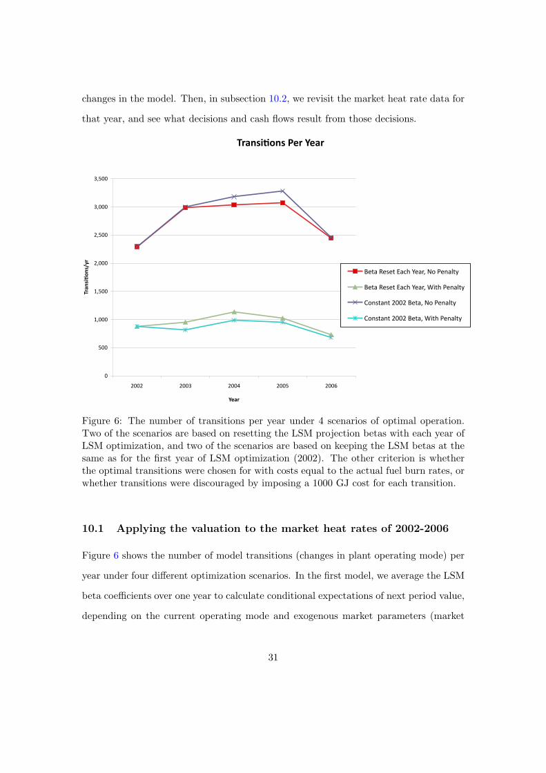
Figure 6: The number of transitions per year under 4 scenarios of optimal operation.Two of the scenarios are based on resetting the LSM projection betas with each year ofLSM optimization, and two of the scenarios are based on keeping the LSM betas at thesame as for the first year of LSM optimization (2002). The other criterion is whetherthe optimal transitions were chosen for with costs equal to the actual fuel burn rates, orwhether transitions were discouraged by imposing a 1000 GJ cost for each transition.
10.1 Applying the valuation to the market heat rates of 2002-2006
Figure 6 shows the number of model transitions (changes in plant operating mode) per
year under four different optimization scenarios. In the first model, we average the LSM
beta coefficients over one year to calculate conditional expectations of next period value,
depending on the current operating mode and exogenous market parameters (market
31

heat rate, time of day, day of week and month of year). This is used on each simulation
path to determine an optimal sequence of operation decisions. This corresponds to
“Beta Reset Each Year, No Penalty”. This is how the model would work if the analyst
recalibrates the LSM model annually.
The first model has two deficiencies. First, it generated many more operating mode
transitions than were customarily used for this type of plant, and there was concern that
it might impose excessive wear and tear on the equipment. Second, the company was
interested in a model that did not require annual recalibration.
To address the first problem, we considered a variation of the model where a 1000 GJ
penalty was imposed on each operating mode transition, to reduce the number of mode
transitions. With typical gas prices of $6/GJ, this corresponds to a $6000 penalty for
changing the operating mode, which the company regarded as a reasonable estimate of
incremental costs from wear and tear. To address the second problem, we estimated the
average LSM conditional expectation betas for 2002 and also used them for determining
optimal decisions in the subsequent years, without re-estimating the LSM model.
Incorporating only the first variation yields the model “Beta Reset Each Year, with
Penalty”. This operating model reduces the number of transitions per year from a range
of 2500 to 3300 down to a range of approximately 1000, which is slightly less than 3
transitions per day.
Incorporating only the second variation yields the model “Constant 2002 Beta, No
Penalty”, and this gives almost the same number of transitions per year as the base
model. Incorporating both variations together yields the fourth model “Constant 2002
Beta, With Penalty”. This latter model gives almost the same number of transitions as
the penalty model where the betas are re-estimated annually.
Thus, introducing the penalty for transitions does reduce the number of transitions,
but there is little change in the number of transitions arising from the policy of using
the betas from 2002, rather than re-estimating each year.
32

Generally, there are more transitions in the middle years, which also had the lowest
heat rates. The no-penalty model generated the highest number of transitions in 2005,
which is a low heat rate year. Interestingly, this had more transitions than 2006, which
is the year with the most power price spikes.6 Thus, volatility (or spikes) do not induce
as many transitions (flexible behaviour), as we might initially expect for a real options
model. This is likely because the year 2006 had a generally high heat rate, so the
volatility apparently did not result in a large number of low market heat rates, where it
would be optimal to turn the power plant off. Indeed, Figure 12 shows that in 2006, the
power plant would be at full output 65% to 75% of the time, depending on the model
used, so there would have been little reason to transition the plant to a lower production
mode.
In contrast, there were a lot of transitions in 2005, which had a low market heat rate,
because the real option flexibility can be used to ramp up the plant and capture the few
periods where running the plant is optimal.
Figure 7 shows the amount of power generated each year under the 4 different models.
The first broad observation to make is that the plant would generate more power in the
early and late years than it would in the middle years. This is consistent with the U-
shaped graph of average market heat rates Y that is shown in Table 1. In the middle
years, the market heat rates were low and optimal operation had the plant shut down
much of the time. Generally speaking, the penalty models tended to have the plant
generating more power than the non-penalty models.7
Figure 8 shows the annual gross margin associated with each of the four strategies.
To make the penalty models comparable to the no-penalty models, we added back the
1000 GJ per transition penalty to the gross margin of the penalty models. That is, the
penalty was used only to change behaviour, rather than reported profit.6Table 1 shows the highest standard deviation for 2006, for example.7Except for the penalty model with the beta being reset each year, and only for the year 2005, where
the power generated is quite low. Clearly, the plant is being shut down completely for much of that year.
33

!"#$%&'$($%)*$+
!
"!!#!!!
$!!#!!!
%!!#!!!
&!!#!!!
'!!#!!!
(!!#!!!
)!!#!!!
*!!#!!!
+!!#!!!
$!!$ $!!% $!!& $!!' $!!(
,$)%
-./01%
,-./01-2-.03/4506-/7#0890:-;/<.=
,-./01-2-.03/4506-/7#0>?.50:-;/<.=
@9;2./;.0$!!$0,-./#0890:-;/<.=
@9;2./;.0$!!$0,-./#0>?.50:-;/<.=
Figure 7: The amount of power generated per year under 4 scenarios of optimal op-eration. Two of the scenarios are based on resetting the LSM projection betas witheach year of LSM optimization, and two of the scenarios are based on keeping the LSMbetas at the same as for the first year of LSM optimization (2002). The other criterionis whether the optimal transitions were chosen for with costs equal to the actual fuelburn rates, or whether transitions were discouraged by imposing a 1000 GJ cost for eachtransition.
34

!""#$%&'()**&+$(,-"&.'/0
!
"#!!!#!!!
$#!!!#!!!
%#!!!#!!!
&#!!!#!!!
'#!!!#!!!
(#!!!#!!!
$!!$ $!!% $!!& $!!' $!!(
12$(
'()**&+
$(,-"&'/34(
)*+,-.*/*+-0,12-3*,4#-56-7*8,9+:
)*+,-.*/*+-0,12-3*,4#-;<+2-7*8,9+:
=68/+,8+-$!!$-)*+,#-56-7*8,9+:
=68/+,8+-$!!$-)*+,#-;<+2-7*8,9+:
Figure 8: The annual gross margin (in GJ) under 4 scenarios of optimal operation. Twoof the scenarios are based on resetting the LSM projection betas with each year of LSMoptimization, and two of the scenarios are based on keeping the LSM betas at the sameas for the first year of LSM optimization (2002). The other criterion is whether theoptimal transitions were chosen for with costs equal to the actual fuel burn rates, orwhether transitions were discouraged by imposing a 1000 GJ cost for each transition.
35

Two things stand out with this graph. First, the gross margin is U-shaped, just like
the market heat rates, so the power plant generates more profit when heat rates are
high, which is no surprise. What may seem more surprising, however, is that the gross
margin is quite insensitive to the precise operating model used.
The fact that the profit margin is not sensitive to changes in the operating strategy,
under optimal operations, arises in this case because the transitions that are avoided
with the penalty model are those where the market heat rate was very close to the plant
heat rate. Thus, the number of transitions can be reduced significantly, if the operator
allows a plant to stay on even if the profit margin (spark spread) has temporarily turned
negative. The losses in this case are not significant. Similarly, the penalty model keeps
the plant from turning on to capture very small positive spark spreads, but missing these
opportunities is not very costly in terms of overall profit.
The fact that the optimal value still stays near the optimum even when the decision
rules are changed from the optimum is a result of the “smooth pasting condition” in this
real options model of operating a plant. The smooth pasting condition is a condition of
optimality and it says, that, when the plant is operated near the optimum, infinitesimal
changes in policy do not affect value (gross margin). Significant changes in policy can
affect value, and the only way to be sure is to compute the value under the optimal and
adjusted policy, as we do here.
Figure 9 shows how often the model has the plant completely shut down (“Cold
Metal”) for each of the 4 years and for each of the 4 operating models. Note that the
penalty models do not let the plant shut down, but the no-penalty models will allow it
to shut down between 10% and 25% of the time. The no-penalty models would have
been more likely to shut the plant down in the middle years when the market heat rate
was low. The times when these models shut down the plant must have been mainly at
the margin of indifference between running and shutting down, because the two different
strategies led to very similar valuations in Figure 8.
36

Percentage of Time Producing 0MW
0%
5%
10%
15%
20%
25%
30%
2002 2003 2004 2005 2006
Year
Beta Reset Each Year, No
Penalty
Beta Reset Each Year, With
Penalty
Constant 2002 Beta, No Penalty
Constant 2002 Beta, With
Penalty
Figure 9: Proportion of time spent in the 0MW “Cold Metal” operating mode for eachof the 4 operating models and operating years.
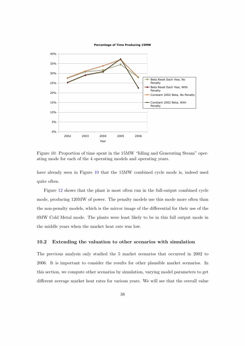
Figure 10 shows that all of the models would have had the plant idling at 15MW in
all years. In this case the stragegies led to essentially the same proportion of time idling,
with greater variation occurring for different years with different heat rates. The plant
was more likely to be running at idle in 2005 when market heat rates were particularly
low, and less likely in the other years with higher heat rates.
Figure 11 shows that none of the models tended to let the plant run in full gas turbine
mode, since this mode occurred in all years for all models less than 1% of the time. This
is particularly interesting, since the 95MW gas turbine mode is a peaking mode that
makes great use of the plant’s ability to ramp up quickly. The operator would enter this
mode if there is a surprising spike in the heat rate — the surprise is needed, since if the
spike is predictable (based on time of day, week or year), the operator would also put
it into combined cycle mode beforehand, and we would see the plant switching between
the 15MW combined cycle mode and the 120MW full output combined cycle mode. We
37
Percentage of Time Producing 15MW
0%
5%
10%
15%
20%
25%
30%
35%
40%
2002 2003 2004 2005 2006
Year
Beta Reset Each Year, No
Penalty
Beta Reset Each Year, With
Penalty
Constant 2002 Beta, No Penalty
Constant 2002 Beta, With
Penalty
Figure 10: Proportion of time spent in the 15MW “Idling and Generating Steam” oper-ating mode for each of the 4 operating models and operating years.
have already seen in Figure 10 that the 15MW combined cycle mode is, indeed used
quite often.
Figure 12 shows that the plant is most often run in the full-output combined cycle
mode, producing 120MW of power. The penalty models use this mode more often than
the non-penalty models, which is the mirror image of the differential for their use of the
0MW Cold Metal mode. The plants were least likely to be in this full output mode in
the middle years when the market heat rate was low.
10.2 Extending the valuation to other scenarios with simulation
The previous analysis only studied the 5 market scenarios that occurred in 2002 to
2006. It is important to consider the results for other plausible market scenarios. In
this section, we compute other scenarios by simulation, varying model parameters to get
different average market heat rates for various years. We will see that the overall value
38

Percentage of Time Producing 95MW
0.0%
0.5%
1.0%
2002 2003 2004 2005 2006
Year
Beta Reset Each Year, No
Penalty
Beta Reset Each Year, With
Penalty
Constant 2002 Beta, No Penalty
Constant 2002 Beta, With
Penalty
Figure 11: Proportion of time spent in the 95MW “Full Gas Turbine” operating modefor each of the 4 operating models and operating years.
is mainly dependent on the average heat rate for the year. Other market issues such as
the frequency of spikes are important, but not as much as the heat rate.
To value a yearly operation of power plants, we must run a given number of simu-
lations of one year of hourly market heat rates. Note this gives 8760 hourly prices per
simulation. The number of simulations we chose is 500; we found this was a reasonable
tradeoff in computation time and accuracy. Once the 500 simulations are done, we can
perform LSM to find a value for each power plant. There are a few items/questions that
must still be addressed:
• We must generate the present value for cash flows greater than a year.
• How do we choose a stylized year? The years 2002-2006 were widely varied in
average market heat rates and spike occurrences.
• How can the modeler compute the year’s plant value for heat rate forecasts that
39

Percentage of Time Producing 120MW
0%
10%
20%
30%
40%
50%
60%
70%
80%
90%
2002 2003 2004 2005 2006
Year
Beta Reset Each Year, No
Penalty
Beta Reset Each Year, With
Penalty
Constant 2002 Beta, No Penalty
Constant 2002 Beta, With
Penalty
Figure 12: Proportion of time spent in the 120MW “Full Combined Cycle” operatingmode for each of the 4 operating models and operating years.
are different than the average heat rate for the stylized years?
It turns out that there is a simple solution to all three of these concerns. We chose
to run the valuations for all 5 stylized years and then altered the mean regime heat
rates by adding and subtracting constants to the intercept of the estimated regime
regressions. Specifically, we add and subtract 1%, 2%, 5%, and 10% to the intercept
term in equation (1). This implies the mean heat rates of the simulations will be different
which will lead to different simulated valuations. This leads to a sequence of expected
heat rates and associated power plant values. These are presented in Figure 13, which
plots the observed valuation and the approximated valuation functions for one year of
operations, again denominated in GJ rather than $. The lowest value is obtained when
the plant is always generating power, which is to say that it is a baseload plant. It
represents the value of the plant without any option value. The upper values correspond
to the plant being operated optimally. As the mean heat rates become very high, the
40

two values converge to each other because there is little to be gained by shutting down
the plant when the heat rate is high. We also fit a fourth order polynomial to fit the
points of the optimal valuation. When the plant is operated as a baseload plant, we can
see that the gross margin is linear in the mean market heat rate, much like the intrinsic
value of an option. But, when it is allowed to operate optimally, the downside losses
at low heat rates are mitigated and the overall value rises. The polynomial fit gives an
increasing convex function over the relevant range, much like an option value lies about
the underlying intrinsic value of the option.
In the five years of actual data, the average market heat rate and the probability of a
spike varied, as can be seen from the regression and logit models of Table 2, where each
of the years 2003 to 2006 had a distinctly different combination of mean (in the dummy
variable) heat rate and mean in the logistic regression. The base year was 2002, and the
other years had a lower mean heat rate in the non-spike regime, and all but 2006 had
the same or lower mean heat rate in the spike regime, as can be seen from the dummy
variables for those years. But, the dummy variable for the logistic regression has both
positive and negative dummy variables, indicating higher or lower probabilities of spikes.
For example, the years 2003 and 2004 have the same mean heat rate in the non-spike
regime, but 2003 has a much higher probability of a spike.
This suggests that the real option values for these years might generally vary along
two dimensions: mean heat rate for the year and number of spikes in the year. When
we plotted the data for alternative regimes in Figure 13, we only varied the mean heat
rate for the year, and not the mean probability of a spike. If the spike probability is
actually a major determinant of option value, we would expect that many option values
would plot off the smooth curve of Figure 13, because the explanatory variable there
was only mean market heat rate, and not mean probability of a spike. But, looking at
the graph, we can see that all of the optimal operation estimates plot closely to one
smooth curve, which means that the major explanatory variable in the option value was
41

-2
0
2
4
6
8
10
8 9 10 11 12 13 14 15 16 17 18
Valu
e (
GJ x
10
^6
)
Mean Market Heat Rate GJ/MWh
Annual Plant Gross Margin (units of million GJ of Gas)
Optimal Operation
Baseload
Operation
Polynomial Fit
Figure 13: Valuation of the two power plant as a function of average yearly heat rates.The upper curve is a polynomial fit to the simulated value when the plant is run opti-mally. The lower circles are simulated values when the plant is always on, as in baseloadoperation. The option value lifts the value above the baseload value, but the value gainis reduced when the market heat rate is high.
42

the mean market heat rate for the year, rather than the probability of spikes for the
year. This confirms the observation we made in the introductory Section 1.
11 Conclusion
This paper has analyzed power plant operating in Alberta that is based on two General
Electric LM6000 gas turbines, that can also generate steam power from the exhaust
gases.
We have found that the gross margins for the plants are sensitive to market condi-
tions, such as the average heat rate for the year. However, they are not very sensitive
to varying the strategy to reduce the amount of plant cycling. We have shown that
the operating rules can be modified to cut the number of plant transition cycles in half
without significantly impairing plant financial performance.
43

References
Alesii, G. (2005). VaR in real options analysis. Review of Financial Economics,
14(3/4):189–208.
Alesii, G. (2008). Assessing Least Squares Monte Carlo (LSMC) for the Kulatilaka
Trigeorgis general real options pricing model.
Black, F. and Scholes, M. (1973). The pricing of options and corporate liabilities. Journal
of Political Economy, 81(3):637–654.
Broadie, M. and Glasserman, P. (1997). Pricing american-style securities using simula-
tion. Journal of Economic Dynamics and Control, 21(8-9):1323–1352.
Calistrate, D., Paulhus, M., and Sick, G. (1999). A recombining binomial-tree for valuing
real options with complex structures. Real Options Conference Netherlands Institute
for Advanced Studies.
Carmona, R. and Durrleman, V. (2003). Pricing and hedging spread options. SIAM
Review, 45(4):627–685.
Cox, J. C., Ingersoll, Jr., J. E., and Ross, S. A. (1985). An intertemporal general
equilibrium model of asset prices. Econometrica, 53(2):363–384.
Cox, J. C., Ross, S. A., and Rubinstein, M. (1979). Option pricing: A simplified ap-
proach. Journal of Financial Economics, 7:229–263.
Deng, S.-J., Johnson, B., and Sogomonian, A. (2001). Exotic electricity options and the
valuation of electricity generation and transmission assets. Decision Support Systems,
30:383–392.
Elliott, R., Sick, G., and Stein, M. (2002). Price interactions of baseload supply changes
and electricity demand shocks. In Ronn, E. I., editor, Real Options and Energy Man-
44
agement: Using Options Methodology to Enhance Capital Budgeting Decisions, chap-
ter 12, pages 371–391. Risk Waters Group, London.
Fleten, S.-E. and Nasakkala, E. (2010). Gas-fired power plants: Investment timing,
operating flexibility and CO2 capture. Energy Economics, 32(4):805–816.
Gardner, D. and Zhuang, Y. (2000). Valuation of power generation assets: A real options
approach. Algo Research Quarterly, 3(3):9–20.
Glasserman, P. (2003). Monte Carlo Methods in Financial Engineering, volume 53 of
Stochastic Modelling and Applied Probability. Springer-Verlag.
Goto, M. and Karolyi, G. A. (2004). Understanding electricity price volatility within
and across markets.
Heydari, S. and Siddiqui, A. (2010). Valuing a gas-fired power plant: A comparison
of ordinary linear models, regime-switching approaches, and models with stochastic
volatility. Energy Economics, 32(3):709–725.
Hlouskova, J., Kossmeier, S., Obersteiner, M., and Schnabl, A. (2005). Real options and
the value of generation capacity in the german electricity market. Review of Financial
Economics, 14(3/4):297–310.
Howison, S. and Coulon, M. C. (2009). Stochastic behaviour of the electricity bid stack:
From fundamental drivers to power prices. The Journal of Energy Markets, 2(1).
Huisman, R. and Mahieu, R. (2003). Regime jumps in electricity prices. Energy Eco-
nomics, 25(5):425–434.
Kamat, R. and Oren, S. S. (2002). Exotic options for interruptible electricity supply
contracts. OPERATIONS RESEARCH, 50(5):835–850.
45

Kanamura, T. and Ohashi, K. (2007). A structural model for electricity prices with
spikes: Measurement of spike risk and optimal policies for hydropower plant operation.
Energy Economics, 29(5):1010–1032.
Kulatilaka, N. (1993). The value of flexibility: The case of a dual-fuel industrial steam
boiler. Financial Management, 22(3):271–280.
Longstaff, F. A. and Schwartz, E. S. (2001). Valuing american options by simulation: a
simple least-squares approach. The Review of Financial Studies, 14(1):113–147.
Margrabe, W. (1978). The value of an option to exchange one asset for another. Journal
of Finance, 33(1):177–186.
Martzoukos, S. H. (2001). The option on n assets with exchange rate and exercise price
risk. Journal of Multinational Financial Management, 11:1–15.
McDonald, R. and Siegel, D. (1984). Option pricing when the underlying asset earns a
below-equilibrium rate of return: A note. The Journal of Finance, 39(1):261–265.
Mount, T. D., Ning, Y., and Cai, X. (2006). Predicting price spikes in electricity markets
using a regime-switching model with time-varying parameters. Energy Economics,
28(1):62–80.
Nasakkala, E. and Fleten, S.-E. (2005). Flexibility and technology choice in gas fired
power plant investments. Review of Financial Economics, 14(3-4):371–393.
Seifert, J. and Uhrig-Homburg, M. (2007). Modelling jumps in electricity prices: theory
and empirical evidence. Review of Derivatives Research, 10(1):59–85.
Sick, G. A. (1989). Capital budgeting with real options. Monograph Series in Finance
and Economics, (1989-3):1–78.
46

Sick, G. A. (1995). Real options. In Jarrow, R., Maksimovic, V., and Ziemba, W. T.,
editors, Finance, volume 9 of Handbooks in Operations Research and Management
Science, chapter 21, pages 631–691. North Holland.
47