Embed Size (px)
Citation preview

Valorization of waste heat in the
food industry
A thermo-economic-environmental analysis of heat recovery technologies in
a milk powder factory
by
T.A. Rigter


VA LO R I Z AT I O N O F W A S T E H E AT I N T H E F O O D I N D U S T R YA T H E R M O - E C O N O M I C - E N V I R O N M E N TA L A N A LY S I S O F H E AT
R E C O V E R Y T E C H N O LO G I E S I N A M I L K P O W D E R FA C TO R Y
by
T.A. Rigter
June 2020
A thesis submitted to the Delft University of Technology & Leiden University in partialfulfillment
of the requirements for the degree of
Master of Sciencein Industrial Ecology
at the Delft University of Technology, to be defended publicly and online on Friday June19, 2020 at 14:30.
Supervisors: Dr.ir. G. Korevaar (TU Delft)Dr.ir. C.A. Infante Ferreira (TU Delft)T.W.M Hermens van Ruremonde (Royal FrieslandCampina N.V.)

E X E C U T I V E S U M M A R Y
This study provides suggestions to decrease hot utility use and impact on the en-vironment of a skim milk powder (SMP) processing plant. These suggestions arebased on the integration of waste streams with processes in the production of SMP.To identify appropriate waste and process streams, process integration has provento be a successful method. This concept addresses the issue of waste heat of aprocess by pointing out to the importance of the relation between unit-processes.In this study, the integration of waste streams is accomplished by heat exchangers,heat pumps and a zeolite wheel. The general assumption underlying this research,is that recovering heat from unused waste streams decreases hot utility use.
Multiple methodologies were used in this study. To accomplish process integra-tion, the pinch analysis forms an essential tool. This analysis was used to identifypotential heat recovery schemes in the SMP plant. Furthermore, to fully understandthese schemes, a thermal, environmental and economical analysis was done. Theseanalyses were based on mass and energy balances, (in)direct CO2 emissions andinvestment and operational costs.
Several conclusion can be drawn from the pinch analysis. First, the pinch tem-perature is 50
C. This represents the dividing line between processes which requireheating and cooling. Second, the heating and cooling demand is known. The SMPproduction process requires 6.8 MW of external heating and 1.7 MW of externalcooling. Third, the amount of recoverable heat is equal to 5.3 MW. Fourth, appro-priate heat sink and sources are identified. The heat sources, i.e. waste streams, arethe spray dryer exhaust and the the condensate streams from two evaporators. Thesupply temperatures of the exhaust and the condensate streams are respectively77, 65 and 55
C. The appropriate heat sinks are the spray dryer air inlet and theevaporator product inlet streams. The target temperature of the spray dryer inletand evaporator inlet streams are respectively 190, 75 and 70
C. Seven heat recoverysetups are proposed.
In terms of saved energy, the spray dryer exhaust has the most potential for heatrecovery. The zeolite wheel is the best performing heat recovery technology in thespray dryer process, with a recovery of 3.5 MW. Furthermore, a heat exchanger-heatpump combination and a stand-alone heat exchanger recover respectively 1.8 and1.6 MW. In contrast, the evaporation process has less potential for heat recovery.The best performing configuration is a heat pump, recovering 1.4 MW from theevaporator condensate.
The environmental performance is strongly related with the amount of energysaved. This is because the most decisive parameter in the environmental analysisis the carbon intensity of natural gas and electricity. The best performing config-urations in terms of saved CO2 emissions are the zeolite wheel (3806 ton/yr), theheat exchanger-heat pump combination (1934 ton/yr) and the stand-alone heat ex-changer (1593 ton/yr) in the spray dryer process. In the evaporation section, theheat pump saves 1485 ton CO2 per year.
The total annual costs are derived from the equivalent annual costs of the asset,carbon savings and utility savings/costs. The best performing configuration is theheat pump in the evaporation process. This technology has an annual return of 145
ke per year. Other configurations with a high return are the stand-alone heat ex-
v

changer (143 ke/yr), the heat exchanger-heat pump combination (128 ke/yr) andthe zeolite wheel (123 ke/yr).
The following recommendations can be listed:
• To save the most energy and CO2 emissions in the spray dryer process, thezeolite wheel proves to be the best technology. Annually, the wheel saves 3.5MW and 3806 ton CO2.
• To achieve the highest economic returns in the spray dryer process, the stand-alone heat exchanger is the best technology. Annually, the heat exchangerpotentially saves 143 ke/year.
• In the evaporation section, the heat pump is the best performing configura-tions, with annual savings of 1.4 MW, 1485 ton CO2 and 145 ke returns.
Some of the limitations of this study are listed below:
• The model is based on ideal conditions. This means that the projected resultsmay difer from actual effects of technologies.
• The effects of the zeolite wheel and the heat pump in the evaporation sectionare based on the fact that heat surplus is used. However, the results do nottake into account the investment costs and CO2 emissions associated with apotential heat exchanger to recover this heat surplus.

A C K N O W L E D G E M E N T S
After six months of hard work in the picturesque village of Bedum, I proudlypresent my research. I couldn’t have made this possible on my own and that’swhy I want to thank some people. First of all, I would like to thank Tessa for pro-viding me the opportunity to do my research and for being such a kind personthroughout my internship. Furthermore, I would like to thank all the people at thefactory with whom I worked closely. Especially Marco and Manon, for pointing mein the right direction when it was needed.
I would like to thank my academic supervisors. Thanks to Gijsbert for reflectingon my work. And thanks to Carlos, especially for his feedback on the heat pumpcalculations.
Lastly, my sincere appreciation for my family and friends for their support through-out my seemingly endless time at the university.
Tom Ayolt RigterAmsterdam, June 2020
vii


C O N T E N T S
1 introduction 1
1.1 Objective . . . . . . . . . . . . . . . . . . . . . . . . . . . . . . . . . . . . 2
1.2 Research question . . . . . . . . . . . . . . . . . . . . . . . . . . . . . . . 3
2 background 5
2.1 Heat recovery in the dairy industry by heat exchangers . . . . . . . . . 5
2.2 Heat recovery by heat pumps . . . . . . . . . . . . . . . . . . . . . . . . 6
2.3 Heat recovery by zeolite wheels . . . . . . . . . . . . . . . . . . . . . . . 7
2.4 Technology background . . . . . . . . . . . . . . . . . . . . . . . . . . . 10
2.4.1 Heat exchanger . . . . . . . . . . . . . . . . . . . . . . . . . . . . 10
2.4.2 Vapor compression heat pump . . . . . . . . . . . . . . . . . . . 11
2.4.3 Mechanical vapor recompression . . . . . . . . . . . . . . . . . . 12
2.4.4 Zeolite wheel . . . . . . . . . . . . . . . . . . . . . . . . . . . . . 13
3 methodology 17
3.1 Case study . . . . . . . . . . . . . . . . . . . . . . . . . . . . . . . . . . . 18
3.1.1 Milk treatment . . . . . . . . . . . . . . . . . . . . . . . . . . . . 18
3.1.2 Evaporation . . . . . . . . . . . . . . . . . . . . . . . . . . . . . . 19
3.1.3 Spray dryer . . . . . . . . . . . . . . . . . . . . . . . . . . . . . . 20
3.2 Pinch analysis . . . . . . . . . . . . . . . . . . . . . . . . . . . . . . . . . 21
3.2.1 Data extraction . . . . . . . . . . . . . . . . . . . . . . . . . . . . 21
3.2.2 Stream selection . . . . . . . . . . . . . . . . . . . . . . . . . . . 22
3.2.3 Intermediate and end-units . . . . . . . . . . . . . . . . . . . . . 23
3.2.4 Mixing of streams . . . . . . . . . . . . . . . . . . . . . . . . . . 23
3.2.5 Composite curves . . . . . . . . . . . . . . . . . . . . . . . . . . . 24
3.2.6 Grand Composite Curve . . . . . . . . . . . . . . . . . . . . . . . 26
3.3 Identifying HEX recovery options . . . . . . . . . . . . . . . . . . . . . 27
3.4 Graphical approach of heat pump integration . . . . . . . . . . . . . . 29
3.5 Identifying HP heat recovery options . . . . . . . . . . . . . . . . . . . 31
3.6 Integration of zeolite wheel . . . . . . . . . . . . . . . . . . . . . . . . . 33
3.7 Environmental analysis . . . . . . . . . . . . . . . . . . . . . . . . . . . 33
3.8 Economic analysis . . . . . . . . . . . . . . . . . . . . . . . . . . . . . . 33
3.9 Data . . . . . . . . . . . . . . . . . . . . . . . . . . . . . . . . . . . . . . . 34
3.9.1 Mass flow rate and temperature . . . . . . . . . . . . . . . . . . 34
3.9.2 Specific heat capacity . . . . . . . . . . . . . . . . . . . . . . . . 35
3.9.3 Minimum temperature difference . . . . . . . . . . . . . . . . . 35
3.9.4 Properties of dairy produts . . . . . . . . . . . . . . . . . . . . . 36
3.9.5 Time . . . . . . . . . . . . . . . . . . . . . . . . . . . . . . . . . . 36
3.9.6 Heat transfer coefficient . . . . . . . . . . . . . . . . . . . . . . . 36
3.9.7 HP specifications . . . . . . . . . . . . . . . . . . . . . . . . . . . 36
3.9.8 Adsorption heat . . . . . . . . . . . . . . . . . . . . . . . . . . . 36
3.9.9 Environmental data . . . . . . . . . . . . . . . . . . . . . . . . . 36
3.9.10 Economic data . . . . . . . . . . . . . . . . . . . . . . . . . . . . 38
3.10 Mass and energy balances . . . . . . . . . . . . . . . . . . . . . . . . . . 38
4 results 39
4.1 Energy map . . . . . . . . . . . . . . . . . . . . . . . . . . . . . . . . . . 39
4.2 Process flow sheet for pinch analysis . . . . . . . . . . . . . . . . . . . . 40
4.3 Composite curves . . . . . . . . . . . . . . . . . . . . . . . . . . . . . . . 44
4.4 Grand Composite Curve . . . . . . . . . . . . . . . . . . . . . . . . . . . 47
4.5 Energy assessment of HEX, HP and zeolite wheel . . . . . . . . . . . . 50
4.5.1 Spray dryer exhaust indirect HEX heat recovery (option 1) . . . 50
4.5.2 Spray dryer exhaust direct HEX heat recovery (option 2) . . . . 52
4.5.3 Evaporator II condensate HEX recovery (option 3) . . . . . . . 52
ix

x contents
4.5.4 Spray dryer exhaust with HEX and HP recovery (option 4) . . 53
4.5.5 Evaporator I condensate HP recovery (option 5) . . . . . . . . . 55
4.5.6 Evaporator II condensate HP recovery (option 6) . . . . . . . . 57
4.5.7 Spray dryer exhaust zeolite wheel recovery (option 7) . . . . . 59
5 sensitivity analysis 63
6 discussion 65
6.1 Discussion of the model and input data . . . . . . . . . . . . . . . . . . 65
6.2 Discussion of results . . . . . . . . . . . . . . . . . . . . . . . . . . . . . 66
6.3 Discussion of results in comparison with existing literature . . . . . . 69
7 conclusion 71
a milk treatment 78
b evaporation 79
c spray drying 80
d heating and cooling 81
e state points of options 82
f input parameters for the zeolite wheel 84
g zeolite state points 85
h results of upper and lower case 86

L I S T O F F I G U R E S
Figure 1.1 Cumulative EU production of different dairy products from1990 to 2019 . . . . . . . . . . . . . . . . . . . . . . . . . . . . . 1
Figure 2.1 Schematic heat exchanger. . . . . . . . . . . . . . . . . . . . . . 10
Figure 2.2 Schematic vapor compression heat pump. . . . . . . . . . . . . 11
Figure 2.3 Schematic mechanical vapor recompression unit. . . . . . . . 12
Figure 2.4 Zeolite wheel with adsorption, regeneration and heating/-cooling . . . . . . . . . . . . . . . . . . . . . . . . . . . . . . . . 13
Figure 2.5 Schematic Zeolite Wheel . . . . . . . . . . . . . . . . . . . . . . 14
Figure 3.1 Research flow diagram . . . . . . . . . . . . . . . . . . . . . . . 18
Figure 3.2 Raw milk treatment . . . . . . . . . . . . . . . . . . . . . . . . . 19
Figure 3.3 Evaporation section . . . . . . . . . . . . . . . . . . . . . . . . . 20
Figure 3.4 Spray drying section . . . . . . . . . . . . . . . . . . . . . . . . 21
Figure 3.5 Original process flow of preheating skim milk. . . . . . . . . . 22
Figure 3.6 Data extraction for subdivided streams. . . . . . . . . . . . . . 23
Figure 3.7 Streams entering a mixer . . . . . . . . . . . . . . . . . . . . . . 24
Figure 3.8 Data extraction for mixed streams. . . . . . . . . . . . . . . . . 24
Figure 3.9 Construction of hot and cold composite curves. . . . . . . . . 25
Figure 3.10 Shifted composite curves. . . . . . . . . . . . . . . . . . . . . . 25
Figure 3.11 Grand Composite Curve for a process. . . . . . . . . . . . . . . 27
Figure 3.12 Decision tree for HEX integration under specific conditions. . 28
Figure 3.13 Placing an VCHP in the process using the GCC. . . . . . . . . 29
Figure 3.14 Heat pump integration using the GCC. . . . . . . . . . . . . . 30
Figure 3.15 GGC’s with heat pump integration. . . . . . . . . . . . . . . . 30
Figure 3.16 Decision tree for HP integration under specific conditions. . . 32
Figure 3.17 Schematic operations curve. . . . . . . . . . . . . . . . . . . . . 34
Figure 4.1 Heating and cooling demand for case study. . . . . . . . . . . 39
Figure 4.2 Process flow sheet. . . . . . . . . . . . . . . . . . . . . . . . . . 42
Figure 4.3 Mollier chart of SD exhaust . . . . . . . . . . . . . . . . . . . . 44
Figure 4.4 Composite curves. . . . . . . . . . . . . . . . . . . . . . . . . . . 44
Figure 4.5 Grand Composite Curve. . . . . . . . . . . . . . . . . . . . . . . 47
Figure 4.6 GCC and heat pump integration. . . . . . . . . . . . . . . . . . 47
Figure 4.7 Heat recovery configurations . . . . . . . . . . . . . . . . . . . 50
Figure 4.8 Process flow diagram of option 1 . . . . . . . . . . . . . . . . . 51
Figure 4.9 Process flow diagram of option 2 . . . . . . . . . . . . . . . . . 52
Figure 4.10 Process flow diagram of option 3 . . . . . . . . . . . . . . . . . 53
Figure 4.11 Process flow diagram of option 4 . . . . . . . . . . . . . . . . . 54
Figure 4.12 COP curves of option 4 . . . . . . . . . . . . . . . . . . . . . . . 54
Figure 4.13 Process flow diagram of option 5 . . . . . . . . . . . . . . . . . 56
Figure 4.14 COP curves of option 5 . . . . . . . . . . . . . . . . . . . . . . . 56
Figure 4.15 Process flow diagram of option 6 . . . . . . . . . . . . . . . . . 57
Figure 4.16 COP curves of option 6 . . . . . . . . . . . . . . . . . . . . . . . 58
Figure 4.17 Process flow diagram of option 7 . . . . . . . . . . . . . . . . . 59
Figure 4.18 Mollier chart of the airside of an open loop zeolite wheelconfiguration. . . . . . . . . . . . . . . . . . . . . . . . . . . . . 60
Figure 5.1 Relative costs for varying SD inlet temperatures. . . . . . . . . 63
Figure 5.2 Varying COP values for option 4 . . . . . . . . . . . . . . . . . 64
Figure 6.1 Results of study . . . . . . . . . . . . . . . . . . . . . . . . . . . 67
Figure 6.2 Comparison of different options . . . . . . . . . . . . . . . . . 68
xi

L I S T O F TA B L E S
Table 2.1 Summary of scientific literature . . . . . . . . . . . . . . . . . . 9
Table 3.1 Specific heat capacity of substances at ambient temperature. . 35
Table 3.2 Dairy properties. . . . . . . . . . . . . . . . . . . . . . . . . . . 36
Table 3.3 Heat transfer coefficient for different heat exchangers. . . . . . 36
Table 3.4 Mass composition of a zeolite wheel . . . . . . . . . . . . . . . 37
Table 3.5 Environmental data for heat recovery technologies. . . . . . . 37
Table 3.6 Direct carbon intensity of different energy carriers. . . . . . . 38
Table 3.7 Prices of utilities and emitted CO2. . . . . . . . . . . . . . . . . 38
Table 3.8 Input variables for economic analysis. . . . . . . . . . . . . . . 38
Table 3.9 Mass and energy balances of unit-processes. . . . . . . . . . . 38
Table 4.1 Overview of utility consuming units. . . . . . . . . . . . . . . . 40
Table 4.2 Process streams corresponding to process flow sheet. . . . . . 41
Table 4.3 Suitable heat sources for heat recovery based on hot streamrules. . . . . . . . . . . . . . . . . . . . . . . . . . . . . . . . . . 45
Table 4.4 Suitable heat sinks for heat recovery based on hot stream rules. 46
Table 4.5 Heat sink identification for heat pump integration. . . . . . . 48
Table 4.6 Heat source identification following the GCC. . . . . . . . . . 48
Table 4.7 Conditions for appropriate placement of heat pump in process. 49
Table 4.8 Results of option 1 . . . . . . . . . . . . . . . . . . . . . . . . . 51
Table 4.9 Results of option 2 . . . . . . . . . . . . . . . . . . . . . . . . . 52
Table 4.10 Results of option 3 . . . . . . . . . . . . . . . . . . . . . . . . . 53
Table 4.11 Specifications of the heat pump for option 4 . . . . . . . . . . 55
Table 4.12 Results of option 4 . . . . . . . . . . . . . . . . . . . . . . . . . 55
Table 4.13 Specifications of the heat pump for option 5 . . . . . . . . . . 56
Table 4.14 Results of option 5 . . . . . . . . . . . . . . . . . . . . . . . . . 57
Table 4.15 Specifications of the heat pump for option 6 . . . . . . . . . . 58
Table 4.16 Results of option 6 . . . . . . . . . . . . . . . . . . . . . . . . . 58
Table 4.17 Energy balance of adsorption unit . . . . . . . . . . . . . . . . 59
Table 4.18 Zeolite heat requirement overview. . . . . . . . . . . . . . . . . 60
Table 4.19 Results of option 7 . . . . . . . . . . . . . . . . . . . . . . . . . 61
Table A.1 State points of the milk treatment section . . . . . . . . . . . . 78
Table B.1 State points of the evaporation section . . . . . . . . . . . . . . 79
Table C.1 State points of the spray drying section . . . . . . . . . . . . . 80
Table D.1 The heating and cooling demand of the conventional case. . . 81
Table E.1 State points of option 1 . . . . . . . . . . . . . . . . . . . . . . . 82
Table E.2 State points of option 2 . . . . . . . . . . . . . . . . . . . . . . . 82
Table E.3 State points of option 3 . . . . . . . . . . . . . . . . . . . . . . . 82
Table E.4 State points of option 4 . . . . . . . . . . . . . . . . . . . . . . . 82
Table E.5 State points of option 5 . . . . . . . . . . . . . . . . . . . . . . . 83
Table E.6 State points of option 6 . . . . . . . . . . . . . . . . . . . . . . . 83
Table F.1 Zeolite wheel input parameters. . . . . . . . . . . . . . . . . . . 84
Table G.1 State points of the zeolite wheel configuration . . . . . . . . . 85
Table H.1 Results of the optimal case on energy use, environment andeconomy . . . . . . . . . . . . . . . . . . . . . . . . . . . . . . . 86
Table H.2 Results of the lower case on energy use, environment andeconomy . . . . . . . . . . . . . . . . . . . . . . . . . . . . . . . 86
xiii


A C R O N Y M S
EU European Union . . . . . . . . . . . . . . . . . . . . . . . . . . . . . . . . . . . . . . . . . . . . . . . . . . . . . . . . . . . . 1
GHG greenhouse gas . . . . . . . . . . . . . . . . . . . . . . . . . . . . . . . . . . . . . . . . . . . . . . . . . . . . . . . . . . . . . 1
SMP skim milk powder. . . . . . . . . . . . . . . . . . . . . . . . . . . . . . . . . . . . . . . . . . . . . . . . . . . . . . . . . . .1
PM pinch methodology . . . . . . . . . . . . . . . . . . . . . . . . . . . . . . . . . . . . . . . . . . . . . . . . . . . . . . . . . 5
HEN heat exchanger network . . . . . . . . . . . . . . . . . . . . . . . . . . . . . . . . . . . . . . . . . . . . . . . . . . . . . 5
COP coefficient of performance. . . . . . . . . . . . . . . . . . . . . . . . . . . . . . . . . . . . . . . . . . . . . . . . . . .6
SD spray dryer . . . . . . . . . . . . . . . . . . . . . . . . . . . . . . . . . . . . . . . . . . . . . . . . . . . . . . . . . . . . . . . . . 5
MVR mechanical vapor recompressor . . . . . . . . . . . . . . . . . . . . . . . . . . . . . . . . . . . . . . . . . . . . . 7
TVR thermal vapor recompressor . . . . . . . . . . . . . . . . . . . . . . . . . . . . . . . . . . . . . . . . . . . . . . . . 7
HEX heat exchanger . . . . . . . . . . . . . . . . . . . . . . . . . . . . . . . . . . . . . . . . . . . . . . . . . . . . . . . . . . . . . . 8
HP heat pump . . . . . . . . . . . . . . . . . . . . . . . . . . . . . . . . . . . . . . . . . . . . . . . . . . . . . . . . . . . . . . . . . . 8
ZW zeolite wheel . . . . . . . . . . . . . . . . . . . . . . . . . . . . . . . . . . . . . . . . . . . . . . . . . . . . . . . . . . . . . . . . 8
VCHP vapor compression heat pump . . . . . . . . . . . . . . . . . . . . . . . . . . . . . . . . . . . . . . . . . . . . 11
EA exhaust air . . . . . . . . . . . . . . . . . . . . . . . . . . . . . . . . . . . . . . . . . . . . . . . . . . . . . . . . . . . . . . . . . 13
PA processed air . . . . . . . . . . . . . . . . . . . . . . . . . . . . . . . . . . . . . . . . . . . . . . . . . . . . . . . . . . . . . . 13
RM regeneration medium . . . . . . . . . . . . . . . . . . . . . . . . . . . . . . . . . . . . . . . . . . . . . . . . . . . . . . 13
MRC Moisture Removal Capacity . . . . . . . . . . . . . . . . . . . . . . . . . . . . . . . . . . . . . . . . . . . . . . . .14
MRR Moisture Removal Regeneration . . . . . . . . . . . . . . . . . . . . . . . . . . . . . . . . . . . . . . . . . . . 14
dm dry matter . . . . . . . . . . . . . . . . . . . . . . . . . . . . . . . . . . . . . . . . . . . . . . . . . . . . . . . . . . . . . . . . . 19
AH absolute humidity . . . . . . . . . . . . . . . . . . . . . . . . . . . . . . . . . . . . . . . . . . . . . . . . . . . . . . . . . 20
MERcold minimum energy requirement for cooling . . . . . . . . . . . . . . . . . . . . . . . . . . . . . . . 26
MERhot minimum energy requirement for heating . . . . . . . . . . . . . . . . . . . . . . . . . . . . . . . 26
GCC Grand Composite Curve . . . . . . . . . . . . . . . . . . . . . . . . . . . . . . . . . . . . . . . . . . . . . . . . . . . 26
TAC total annual costs . . . . . . . . . . . . . . . . . . . . . . . . . . . . . . . . . . . . . . . . . . . . . . . . . . . . . . . . . . 33
EAC equivalent annual costs . . . . . . . . . . . . . . . . . . . . . . . . . . . . . . . . . . . . . . . . . . . . . . . . . . . . 33
LF Lang Factor . . . . . . . . . . . . . . . . . . . . . . . . . . . . . . . . . . . . . . . . . . . . . . . . . . . . . . . . . . . . . . . . 34
P&ID Process & Instrumentation Diagrams . . . . . . . . . . . . . . . . . . . . . . . . . . . . . . . . . . . . . . 34
CIP cleaning in place . . . . . . . . . . . . . . . . . . . . . . . . . . . . . . . . . . . . . . . . . . . . . . . . . . . . . . . . . . . 35
ASHP air-source heat pump . . . . . . . . . . . . . . . . . . . . . . . . . . . . . . . . . . . . . . . . . . . . . . . . . . . . . 36
WSHP water-source heat pump . . . . . . . . . . . . . . . . . . . . . . . . . . . . . . . . . . . . . . . . . . . . . . . . . . 36
MT milk treatment . . . . . . . . . . . . . . . . . . . . . . . . . . . . . . . . . . . . . . . . . . . . . . . . . . . . . . . . . . . . . 40
EV evaporation . . . . . . . . . . . . . . . . . . . . . . . . . . . . . . . . . . . . . . . . . . . . . . . . . . . . . . . . . . . . . . . . 40
SD spray dryer . . . . . . . . . . . . . . . . . . . . . . . . . . . . . . . . . . . . . . . . . . . . . . . . . . . . . . . . . . . . . . . . . 5
RH relative humidity . . . . . . . . . . . . . . . . . . . . . . . . . . . . . . . . . . . . . . . . . . . . . . . . . . . . . . . . . . 43
SHS super-heated steam . . . . . . . . . . . . . . . . . . . . . . . . . . . . . . . . . . . . . . . . . . . . . . . . . . . . . . . . 59
HT heating . . . . . . . . . . . . . . . . . . . . . . . . . . . . . . . . . . . . . . . . . . . . . . . . . . . . . . . . . . . . . . . . . . . . 81
CL cooling. . . . . . . . . . . . . . . . . . . . . . . . . . . . . . . . . . . . . . . . . . . . . . . . . . . . . . . . . . . . . . . . . . . . .81
HW hot water . . . . . . . . . . . . . . . . . . . . . . . . . . . . . . . . . . . . . . . . . . . . . . . . . . . . . . . . . . . . . . . . . . 81
ST steam . . . . . . . . . . . . . . . . . . . . . . . . . . . . . . . . . . . . . . . . . . . . . . . . . . . . . . . . . . . . . . . . . . . . . . 81
xv

xvi list of tables
G gas . . . . . . . . . . . . . . . . . . . . . . . . . . . . . . . . . . . . . . . . . . . . . . . . . . . . . . . . . . . . . . . . . . . . . . . . .81
IW ice water . . . . . . . . . . . . . . . . . . . . . . . . . . . . . . . . . . . . . . . . . . . . . . . . . . . . . . . . . . . . . . . . . . . 81
CW cold water . . . . . . . . . . . . . . . . . . . . . . . . . . . . . . . . . . . . . . . . . . . . . . . . . . . . . . . . . . . . . . . . . 81

1 I N T R O D U C T I O N
In a world with an increasing population, growing demand for food products isinevitable. As one of the largest products in share, dairy products already playa major role in feeding the world population [1]. With a share of 20% of globalproduction, the European Union (EU) is one of the largest producers of all dairyproducts [2]. The EU dairy production accounts for approximately 500 billion kgper year [3]. Since 1990, the production has increased by 45% (Figure 1.1).
0
100000
200000
300000
400000
500000
600000
Pro
du
ctio
n (
x10
3to
n)
Casein
Whey powder
Whole milk powder
Skim milk powder
Cheese
Butter
Fresh dairy products
Milk
Figure 1.1: Cumulative EU production of different dairy products from 1990 to 2019 [2].
The agricultural sector is associated with a large impact on the environment. Live-stock, feed for livestock, land use and forestry account for 24% of global greenhousegas (GHG) emissions [4]. On EU level, the agricultural sector emits 10% of GHGemissions. Looking at post-farm emissions, the production of milk accounts for2.9% of EU GHG emissions [4]. Because the production of dairy products has anincreasing trend and agriculture is associated with a large share of GHG emissions,ways to reduce the impact on the environment need to be introduced.
To reduce environmental impact, the EU committed itself to decrease carbon emis-sions by 80% in 2050 (compared to the 1990 carbon level) [5]. As an energy intensiveindustry, this EU target will be a challenge for the dairy sector. Reason for this isthe strong dependency on fossil fuels in the dairy sector [6]. Coal and natural gasare used to provide thermal energy for the processing of dairy products. To reachthe target, a possibility is to introduce innovative technologies to reduce the energyconsumption of the dairy industry.
One of the most energy-intensive dairy industries is the production of skim milkpowder (SMP) [7]. In contrast with fluid dairy products, milk or butter, SMP is adried product with a moisture content below 5%. These processes demand thermalenergy. In Europe, the specific energy consumption of SMP production is 8.7-16.4MJ/kg. Reason behind this high energy demand is the pasteurization, evaporationand drying need. Changing a fluid into a powder, requires a large amount of ther-mal energy.
1
2 introduction
Pasteurization is the heat treatment of milk. With pasteurization, the milk is heatedto temperatures around 60-80
C. The objective is to eliminate certain pathogens toincrease food safety. Milk is not only pasteurized at the beginning of the process.During the whole process, milk is pasteurized. This is done by steam-injected heatexchangers.
Evaporation is the concentration of a product feed. By means of steam injection,moisture content in the product is evaporated. The result is a concentrated productwith a low moisture content. Usually, the moisture content of the concentrate is50%. Around 2.3-2.7 MJ of latent heat is required to evaporate 1 kg of water [7, 8].Several techniques are present to reduce the energy consumption of the evaporator.For instance, adding multiple evaporation stages decreases energy use. After steamis used for the first evaporation stage, in the subsequent stages, vapor mist providesthe thermal energy [8]. In this way, evaporation energy is divided by the number ofstages.
After the evaporation stage, a dryer is used to produce a powder-form product.In a dryer, the moisture content is reduced to below 5%. In contrast to the evapora-tor, the product in a dryer comes into direct contact with a drying medium. Oftenthis medium is hot air between 190-230
C. A single-stage dryer requires approxi-mately 6.7 MJ to evaporate 1 kg of water [8].
In order to comply to international CO2 reduction targets, two ways are possible.As the diary processing industry relies on fossil fuels, a shift to renewable energysources may reduce emissions. Another possibility is the reduction in energy con-sumption. A way to reduce thermal energy use, is the introduction of both provenand innovative technologies. In processes with large heating demands, linking heatsinks and sources may reduce thermal energy consumption. Regarding heat sinks,the evaporator and dryer are associated with condensate and exhaust air. Theseflows are labeled as waste streams. However, using heat recovery technologies,those waste streams can be useful in the SMP production. By recovering heat fromwaste streams, the total energy demand may be reduced.
1.1 objectiveThe goal of this study is to research what the effect is of different heat recoverytechnologies on carbon dioxide emissions for a single SMP productions site. Ad-ditionally, the costs coupled to these technologies are calculated. This goal can besplit in multiple smaller tasks. The tasks are: (i) identify heat sources and sinks ofthe SMP production site, (ii) introduce possible heat integration technologies and(iii) assess the effect of these technologies on the basis of energy savings, carbonsavings and cost savings. To reach the first two goals, a pinch analysis will beconducted. The last goal will be reached by means of energy, environmental andeconomic analyses.

1.2 research question 3
1.2 research questionWhat is the effect of different heat recovery technologies on the thermal energy consumption,carbon dioxide emissions and economic costs of a skim milk powder production site?
Sub-questions:
1. What are the heating and cooling demand for a skim milk powder productionsite?
2. Which process streams in a skim milk powder production site are relevant fordoing a pinch analysis?
3. Where in the skim milk powder production process can heat recovery tech-nologies be appropriately placed, after calculating the energy targets of theprocess?


2 B A C KG R O U N D
One way to identify potential heat sinks and sources is done by process integration.This concept addresses the issue of waste heat of a process by pointing out to theimportance of the relation between unit-processes. The goal of process integration isto link heat sources and sinks in order to recover waste heat. To accomplish processintegration, the usage of the pinch methodology (PM) as a method is essential. ThePM was introduced by Linnhoff, Mason and Wardle [9]. They presented a processintegration technique for energy targeting and network integration. In the firstplace, PM sets targets for minimum utility usage. By maximizing internal heatrecovery, the external use of heat duty (i.e. steam, gas) and cooling duty (ice water)can be reduced. Secondly, PM proposes a way to integrate processes in the form ofa heat exchanger network (HEN). According to the energy targets, a framework isconstructed in which heat exchangers form the basis for heat recovery.
2.1 heat recovery in the dairy industry by heatexchangers
The PM is frequently used in order to identify potential heat recovery schemes in thedairy industry. Ample studies used PM for the replacement of fossil fuel by renew-able energy sources in a dairy processing industry. For instance, Yildirim and Genc[10] conducted a thermodynamic analysis including an energy and exergy analysisof a milk powder production process. With the integration of geothermal energy,replacing natural gas, the authors found an overall energy efficiency increase of85%. In their research, energy efficiency was defined as the ratio of energy inputto output. The total energy requirement was 17 MJ per kg milk powder, providedby 228 kg geothermal fluid. Another energy analysis, by Sorguven and Ozilgen[11], researched the replacement of fossil fuels with biodiesel in a dairy processingsite. Replacing fossil fuel with biodiesel would enhance energy efficiency by 3%.Furthermore, they showed that the spray dryer (SD) is the most polluting process interms of CO2 emissions. By using a pinch analysis, Quijera et al. [12] firstly assessedthe potential improvements, secondly assessed the process after implementation ofthese improvements and thirdly evaluated the feasibility of integrating solar ther-mal energy in the system. A total of 71% of natural gas consumption could bereplaced by solar thermal energy. This improvement resulted in annual savings of1176 MWh. Especially in summer months, solar thermal collectors were a feasibleway to provide for hot utility. Altogether, these studies demonstrated that the PMcan be successfully used to investigate the replacement of fossil fuels by renewableenergy.
PM can also be applied to the energy analysis of a process as a whole. Severaltotal site pinch analyses were applied to dairy processes. For instance, Buhler etal. [13] suggested possibilities for heat integration through a pinch analysis. Con-clusion of the analysis stated that internal heat recovery had a small potential, asthe processes were already integrated. Atkins et al. [14] found ways to improvethe integration of individual plants in a large dairy processing site. Different wastestreams were recovered by a HEN. In total, 10.8 MW of heat was recovered. Thediscrepancy in results from the two total studies may be explained by the scope of
5

6 background
research. In the case of Buhler et al. [13], several heat recovery technologies werealready integrated. For instance, different heat pumps already recovered severalwaste streams. However, the spray dryer exhaust was not included in the study byBuhler et al. The study by Atkins et al. [14] did include heat recovery of the spraydryer exhaust by a heat exchanger. This may be one explanation for the differencein results.
The PM can be used to assess the heat recovery potential from a whole site. Addi-tionally, specific unit-processes seem suitable for PM. For instance, the effectivenessof milk coolers was researched [15]. By using heat from the milk coolers for cleaningpurposes, 50-60% of total heat could be recovered from the condensation process.The coefficient of performance (COP) of the whole system increased from 3 to 5.Zooming in on the evaporator component in a dairy process, Walmsley et al. [16]found a reduction of 67% in thermal energy use by integrating streams. They inves-tigated direct and indirect heat recovery options for an evaporator condenser. Byoptimizing soft data from the condenser flows, possibilities for integrating the con-denser in the reminder of the dairy process was researched. Two possibilities wereshown, accounting for a heat recovery of 30%. In sum, investigating and optimizingthe evaporator in dairy processing can lead to decreased energy consumption. Theresults show that it is promising to investigate the possibilities to recover waste heatfrom the evaporator.
Besides waste streams from the evaporator, the exhaust of the spray dryer has beensubject to studies. Atkins et al. [17] specifically looked at heat recovery from thespray dryer outlet. The exhaust was recovered via an intermediate liquid loop. Inthis way, the temperature of the spray dryer inlet air was increased. Emphasiz-ing the risk of heat exchanger fouling due to entrained particles in the exhaust,the target temperature of the exhaust was far above its dew point. Using PM, thethermal energy reduction of the whole was 13%. Golman and Julklang [18] alsoinvestigated the recovery of SD exhaust recovery by introducing a semi-closed loopof the exhaust air. By varying the mass flow rate and temperature of the exhaust,the energy savings were calculated. On average, recovering the exhaust by a heatexchanger, thermal energy consumption of the SD decreased by 60%. The savingswere higher for higher temperatures and flow rates of the exhaust. In contrast to theabovementioned studies, Kockel [19] investigated the recovery of the spray latentheat from the dryer exhaust in a dairy plant. Using heat exchangers, hot utility usewas reduced by 25%. Latent heat was recovered by condensing exhaust air in theheat exchangers. Taking together the results, heat recovery of the spray dryer hasan impact on utility reduction. However, all studies stress the risk of heat exchangerfouling by sticky milk powder in the exhaust.
A wealth of studies demonstrate that PM can be successfully used to assess the in-tegration of renewable energy, increase energy efficiency in total sites and decreaseenergy consumption of evaporators and spray dryers by using heat exchangers. Inthe first place, PM is associated with heat exchangers. Previous studies showedwhat the effect can be on energy use when heat exchangers recover waste heat. Inaddition to heat exchanger, there are other technologies to recover heat. Amongthose technologies are heat pumps and sorption systems.
2.2 heat recovery by heat pumpsHeat pumps are used to recover heat from waste flows. By means of electrical workinput, high temperature heat is produced from waste heat. Both in the dairy andother industries, the effect of heat pumps on energy use is studied. PM proves tobe an important tool to identify areas for heat pump integration. Schlosser et al.

2.3 heat recovery by zeolite wheels 7
[20], Stampfli et al. [21] and Olsen et al. [22] studied the integration of a heat pumpin different industries. All studies demonstrated the significance of a graphical ap-proach to identify possible heat pump integration areas. Furthermore, all studiesshowed a reduction in hot utility use. By formulating temperature requirements,these studies showed how PM can be used to properly integrate a heat pump.
PM and heat pumps can also be combined when looking at a specific part of aprocess. Liew and Walmsley [23] studied the possible applications of heat pumpsto upgrade waste heat from a boiler in a dairy plant. They found that four-effectmechanical vapor recompressor (MVR) heat pumps can recover 14 MW of mediumpressure steam, while two-effect thermal vapor recompressor (TVR) heat pumps re-quired 1 MW of low pressure steam and 2 MW high pressure steam to produce 3
MW of medium pressure steam. Overall, the use of medium pressure steam wassatisfied by the heat pumps, at the expenses of a small addition of high pressuresteam while reducing the demand for low pressure steam. Additionally, Walms-ley et al. [24] quantified potential energy savings. By the appropriate placement ofMVR components, heat from evaporators was reintegrated. Requiring an additionalof 16% electricity, 78% of steam was reduced for the whole site. This resulted in areduction of 24% CO2 emissions. Singh and Dasgupta [25] introduced heat pumpintegration within a refrigeration process in a dairy plant. Waste heat from an am-monia based refrigeration system was used to pre-heat boiler feed-in water usinga heat pump. Available heat from the refrigeration system could heat up boilerfeed-in up to 70
C. Approximately 45% CO2 was reduced, and 37 kW of heat wasrecovered. These studies show different energy savings after heat pump integration.Recovering heat from the evaporate and boiler clearly results in high energy savings.
Besides heat from the evaporator and boiler, the potential to recover heat fromthe spray dryer exhaust was investigated. Krokida and Bisharat [26] proposed asetup in which the exhaust of a spray dryer was recovered by both heat exchang-ers and a heat pump. Using a mathematical model, they found that a the heatpump was able to recover 100% of available thermal waste heat, while a heat ex-changer recovered 25%. Wang et al. [27] investigated a similar setup, in whichspray dryer exhaust was recovered by both heat exchangers and a heat pump. Witha heat pump evaporation temperature of 30
C, 40% of hot utility consumption wasreduced. For a stand-alone heat exchanger, hot utility use reduced by 15%. From aneconomic perspective, the heat exchanger was more desirable. Walmsley et al. [28]found a hot utility reduction of 47% for recovering exhaust heat by a heat pump.Another study which highlights the potential of heat pumps to recover low evap-oration temperatures is from Van de Bor et al [29] . They focused on recoveringwaste heat streams at temperatures between 45-60
C with different types of heatpumps. Highlighting vapor compression heat pumps, 4 MW of heat was producedwith a COP of 4. These three studies show there is a potential for heat pumps torecover exhaust. Additionally, in terms of energy recovery, heat pumps seem botha promising alternative and complementary to heat exchangers.
2.3 heat recovery by zeolite wheelsThe drying unit in a SMP production line consumes approximately 50% of the totalenergy use [7]. The high energy consumption is mainly due to the high inlet tem-perature of dry air. After drying the product, lower temperature humid air leavesthe spray dryer. To increase the energy efficiency, many researchers looked at recov-ering heat from the exhaust air of the spray dryer [30]. The energy efficiency can beimproved by raising the temperature of the exhaust air, dehumidifying the exhaustair or both. Zeolite wheels prove to be an efficient way to increase energy efficiency[30]. Zeolites are the collective name for microporous minerals, which function as a

8 background
sieve. For commercial purposes they are used to adsorb water and water vapor. Asmentioned before, [17, 18, 19] placed a heat exchanger to recover sensible heat fromthe exhaust air. Although this resulted in a reduction in hot utility consumption,risk of fouling of heat exchangers due to entrained particles in the exhaust air wasonly briefly mentioned. The principle behind the zeolite wheel is that hot exhaustair is dehumidified by a sorption material so it can be recycled. By dehumidifyingthe exhaust air, latent heat can be recovered. Especially in dryer sections, in whichhot air streams are being utilized, zeolite wheels have the potential to recover heat.Applying PM, Atuonwu et al. [31], proposed a setup in which sensible heat fromthe spray dryer exhaust was recovered. A reduction of 59% in energy consumptionwas achieved by placing zeolite wheels. Latent heat was not recovered as hot airwas above its dew point. In contrast, Atuonwu et al. [32] recovered both sensi-ble and latent heat. Using PM, they found an energy consumption reduction of55% compared to similar dryers without a zeolite wheel. Similarly, Quijano et al.[33], while latent to sensible heat was converted in a liquid zeolite sorption system,found 99% and 58% energy savings for respectively a closed and open loop system.Moejes et al. [34] proposed a closed-loop solution for the spray drying section witha zeolite wheel. The energy consumption for the spray dryer was reduced from 8.5to 5 MJ per kg product. Djaeni et al. [35] researched the application of multiplezeolite dryers. Thermal energy consumption reduced by 50%. Additionally, Djaeniet al. [36] researched the heat recovery potential for low temperature dryer inlet air(70C). Using a zeolite wheel, the dryer became 10-18% more efficient than standard
dryers. Others found a 45% increase in energy efficiency for low temperature dryers[37]. In contrast to the described work, Madhiyanon et al. [38] found an increasein energy consumption due to installation of a zeolite wheel. The system consistedof two closed-loop air streams, one for drying the product and one for the zeoliteregeneration after adsorption. The increase in energy consumption was assigned tothe high heating demand of dehumidifying the zeolite in the regenerative part ofthe wheel. The drying performance of the system remained the same in compari-son with the base case. As the results of the studies show, zeolite wheels technicallyhave large potential to recover heat from the spray dryer exhaust. Therefore it ispromising to further study the application of a zeolite wheel in the dairy industry.Table 2.1 shows an overview of the discussed literature for a heat exchanger (HEX),heat pump (HP) and zeolite wheel (ZW). The abbreviations ’en’, ’env’ and ’eco’ intabel 2.1 stand for respectively energy, environmental and economical.

2.3 heat recovery by zeolite wheels 9
Tabl
e2.
1:Su
mm
ary
ofsc
ient
ific
liter
atur
eIt
emR
ef.
Tech
n.R
esul
tD
ata
type
Dat
ale
vel
Res
earc
hto
olA
naly
sis
[HEX
][H
P][Z
W]
[En]
[Env
][E
co]
1[1
0]
X8
5%
ener
gyef
ficie
ncy
obse
rvat
iona
lin
dust
rial
plan
tca
seen
ergy
anal
ysis
XX
2[1
1]
Xsp
ray
drye
ris
high
est
inte
rms
ofC
O2
emis
-si
ons
obse
rvat
iona
lPr
oduc
tion
line
ener
gyan
alys
isX
3[1
2]
X1
17
6M
Wh/
yrob
serv
atio
nal
indu
stri
alpl
ant
case
pinc
han
alys
isX
4[1
3]
Xno
savi
ngob
serv
atio
nal
indu
stri
alpl
ant
case
pinc
han
alys
isX
5[1
4]
X1
0.8
MW
ofre
cove
ryob
serv
atio
nal
and
illus
trat
ive
indu
stri
alpa
rkca
sepi
nch
anal
ysis
X
6[1
5]
XC
OP
incr
ease
by1.8
expe
rim
enta
lSi
ngle
cool
syst
emex
peri
men
tX
7[1
6]
XX
67%
ther
mal
ener
gyan
d6
40-8
20
ke/y
rco
stob
serv
atio
nal
Evap
orat
orw
ith
MV
Rpi
nch
anal
ysis
XX
8[1
7]
X1
2-2
0%
hot
utili
tyde
man
dob
serv
atio
nal
Indu
stri
alpl
ant
case
pinc
han
alys
isX
9[1
8]
X6
0%
spra
ydr
yer
ener
gyre
duct
ion
illus
trat
ive
Sing
ledr
yer
mod
elsi
mul
atio
nX
10
[19]
X2
5%
spra
ydr
yer
ener
gyre
duct
ion
obse
rvat
iona
lSi
ngle
drye
rm
odel
sim
ulat
ion
X1
1[2
3]
X1
70-3
40
ke/y
ear
and
86
6-3
22
3kW
illus
trat
ive
(sec
-on
dary
)In
dust
rial
plan
tca
sepi
nch
anal
ysis
XX
12
[24]
XX
78%
utili
tyan
dm
inus
16%
elec
tric
ity,
94
2
ke/y
r,3
41
6tC
O2-e
/yr
obse
rvat
iona
lIn
dust
rial
plan
tca
sepi
nch
anal
ysis
XX
13
[25]
XX
37
kW,4
6%
CO
2an
d3
4%
cost
obse
rvat
iona
lR
efri
gera
tion
plan
ten
ergy
anal
ysis
XX
X1
4[2
6]
XX
heat
reco
very
of4
0%
illus
trat
ive
Sing
ledr
yer
mod
elsi
mul
atio
nX
X1
5[2
7]
XX
redu
ctio
nof
40%
heat
load
illus
trat
ive
Sing
ledr
yer
mod
elsi
mul
atio
nX
X1
6[2
9]
Xco
stsa
ving
sbe
twee
n1
25
-70
6ke
/yr
com
pile
dSi
ngle
heat
pum
pm
odel
sim
ulat
ion
XX
17
[31]
XX
59%
ener
gyco
nsum
ptio
nob
serv
atio
nal
(sec
onda
ry)
Sing
ledr
yer
pinc
han
alys
isX
18
[32]
XX
55%
ener
gyco
nsum
ptio
nob
serv
atio
nal
(sec
onda
ry)
Sing
ledr
yer
pinc
han
alys
isX
19
[33]
XX
58-9
9%
ener
gyco
nsum
ptio
nob
serv
atio
nal
Sing
ledr
yer
mod
elsi
mul
atio
nX
20
[34]
XX
4.9
-8.4
MJ/
kgpr
oduc
tob
serv
atio
nal
Prod
ucti
onlin
epi
nch
anal
ysis
X2
1[3
5]
XX
50%
ther
mal
ener
gyco
nsum
ptio
nn/
aSi
ngle
drye
rpi
nch
anal
ysis
X2
2[3
6]
XX
10-1
8%
ener
gyef
ficie
ncy
n/a
Sing
ledr
yer
pinc
han
alys
isX
23
[37]
X4
5%
ther
mal
ener
gyco
nsum
ptio
nob
serv
atio
nal
(sec
onda
ry)
Sing
ledr
yer
mod
elsi
mul
atio
nX
24
[38]
Xm
inus
11-1
8M
J/kg
expe
rim
enta
lSi
ngle
drye
rex
peri
men
tX
10 background
2.4 technology backgroundThis section describes the working principles of three heat recovery technologies;heat exchanger, heat pump and zeolite wheel.
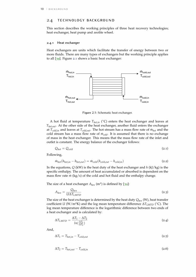
2.4.1 Heat exchanger
Heat exchangers are units which facilitate the transfer of energy between two ormore fluids. There are many types of exchangers but the working principle appliesto all [39]. Figure 2.1 shows a basic heat exchanger:
ṁcold,in
ṁcold,outṁhot,in
ṁhot,outTcold,in
Tcold,outThot,in
Thot,out
Figure 2.1: Schematic heat exchanger.
A hot fluid at temperature Thot,in (C) enters the heat exchanger and leaves atThot,out. At the other side of the heat exchanger, another fluid enters the exchangerat Tcold,in and leaves at Tcold,out. The hot stream has a mass flow rate of mhot and thecold stream has a mass flow rate of mcold. It is assumed that there is no exchangeof mass in the heat exchanger. This means that the mass flow rate of the inlet andoutlet is constant. The energy balance of the exchanger follows:
Qhot = Qcold (2.1)
Following,
mhot(hhot,in − hhot,out) = mcold(hcold,out − hcold,in) (2.2)
In the equations, Q (kW) is the heat duty of the heat exchanger and h (kJ/kg) is thespecific enthalpy. The amount of heat accumulated or absorbed is dependent on themass flow rate m (kg/s) of the cold and hot fluid and the enthalpy change.
The size of a heat exchanger Ahex (m2) is defined by [39]:
Ahex =Qhex
U∆TLMTD(2.3)
The size of the heat exchanger is determined by the heat duty Qhex (W), heat transfercoefficient U (W/m2K) and the log mean temperature difference ∆TLMTD (C). Thelog mean temperature difference is the logarithmic difference between two ends ofa heat exchanger and is calculated by:
∆TLMTD =∆T1 − ∆T2
ln( ∆T1∆T2
)(2.4)
And,
∆T1 = Thot,in − Tcold,out (2.5)
∆T2 = Thot,out − Tcold,in (2.6)

2.4 technology background 11
2.4.2 Vapor compression heat pump
There are several types of heat pumps. In this research the working principle of aclosed cycle vapor compression heat pump (VCHP) and an open cycle MVR will bedescribed. The VCHP is commonly used for industrial applications [29]. The basicset-up of the cycle is a good starting point to understand the working principle ofa heat pump. The VCHP has four components; a compressor, an evaporator, anexpansion valve and a condenser. A working fluid, usually ammonia or an ammo-nia/water mixture, runs through the thermodynamic cycle. The cycle is shown infigure 2.2.
The cycle for an VCHP has four important processes [40]:
• In the evaporator, heat is transferred from a thermal source (Qevap) to theworking fluid. The thermal source can be liquid, gas or ground-sourced. Asheat is transferred, the working fluid evaporates into a saturated vapor atconstant pressure. Both the evaporator and the condenser work as a heatexchanger.
• At low pressure, the saturated vapor enters the compressor. By work (Wel)done in the compressor, the vapor is compressed to a higher pressure andtemperature. It leaves the compressor outlet as superheated vapor.
• The vapor enters the condenser, where heat is rejected to a lower pressureand temperature thermal sink (Qcond). By doing so, the vapor condenses intoa saturated liquid at constant pressure.
• The expansion valve causes a pressure drop, resulting in a lower pressureand temperature of the working fluid. The working fluid usually enters theevaporator as a liquid/vapor mixture.
Evaporator
Condenser
Qevap
Qcond
Wel
compressor
expansion valve
Figure 2.2: Schematic vapor compression heat pump.
From the conservation of energy, the equation follows:
Qcond = Qevap + Wel (2.7)
Where heat output from the condenser Qcond (kW) is equal to the evaporation heatQevap (kW) and work input Wel (kW) [40].
The thermodynamic maximum COP of a heat pump cycle is defined by:
COPcarnot =Tc
Tc − Te(2.8)

12 background
Where COPcarnot (-) is determined by the temperature of the working fluid in thecondenser Tc (Kelvin) and in the evaporator Te (Kelvin).
The actual COP of a heat pump is defined by:
COP = ηTc
Tc − Te=
QcondWel
(2.9)
Where η is the efficiency of the heat pump cycle. The actual COP (-) is defined asthe ratio of heat output from the condenser Qcond to work input Wel. In general, theCOP of heat pumps is used to define performance and to compare this performancewith other heat pumps. A low COP means that the ratio of released heat and workinput is small. On the other hand, when a heat pump has a high COP, more heatis released in comparison with work input. If COP values are greater than 1, thismeans that for every kW of work required, more than 1 kW of heat is released fromthe working fluid in the condenser. A high COP indicates that work input is wortha lot in terms of thermal energy.
2.4.3 Mechanical vapor recompression
In contrast to an VCHP, an MVR is an open cycle heat pump. This means that theworking fluid is not reused. Like an VCHP, an MVR system often consists of acompressor, evaporator and condenser. Figure 2.3 shows a simple setup of an MVRevaporation system, in which a feed stream is concentrated. The only time the MVRrequires steam is at the start of evaporation. Start-up steam is used to evaporatethe first amount of feed. In the evaporator, moisture in the feed is evaporated byindirect contact with steam. Then the steam is condensed and leaves the evaporatoras condensate. The concentrate also leaves the evaporator. The evaporated moisturefrom the feed is used for the evaporation of the following batch. This stream leavesthe evaporator at lower pressure and temperature relative to the start-up steaminjection. A compressor raises pressure and temperature of the process steam. Thecompressed steam enters the evaporator and replaces the start-up steam in the firstround. After steam rejects its latent heat to the feed stream, it leaves as condensate.
Feed
Condensate
Process steam
Compressed steam
MVR
Evaporator
Concentrate
Start-up steam
Figure 2.3: Schematic mechanical vapor recompression unit.

2.4 technology background 13
2.4.4 Zeolite wheel
The energy consumption of spray dryers can be improved by integrating a zeoliteunit to the dryer. In spray drying, hot air is used to drive moisture from a concen-trate to vapor in hot air. The exhaust of the spray dryer is humid air, containingevaporated water from the liquid. As spray drying requires high temperatures, ex-haust air is usually in the range of 60-100
C. As discussed, recuperation of thisexhaust air is a way to recover heat. However, heat recovery is possible up to acertain temperature as condensed exhaust air can decrease the performance of heatexchangers due to sticky entrained particles. When humid exhaust air penetratesa zeolite layer, water molecules are taken up by zeolite molecules. Water uptakefrom the air and the increase in temperature is done by adsorption heat. This typeof heat is released by zeolite material in the wheel. This results in a reduction inenergy consumption, as high temperature dry air can be used in the spray dryer.A downside of the zeolite wheel is the high energy demand for the regenerationof the zeolite. Using hot air or steam as a regeneration medium, water is removedfrom the spent zeolite. The zeolite sorption system is illustrated in figure 2.4.
Figure 2.4: Zeolite wheel with adsorption, regeneration and heating/cooling [34].
The zeolite system has the shape of a wheel and consists of three components:adsorption, regeneration and heater/cooler. The exhaust air passes through theadsorption component, where the zeolite adsorbs the water vapor. The incominghumid air stream contains both sensible and latent heat. Sensible heat is increaseddue to adsorption heat. As the zeolite adsorbs water from the air, adsorption heatis released to the air stream. Additionally, latent heat is recovered due to moistureloss. In the zeolite bed, vapor is condensed, releasing heat to the air. After the ad-sorption section, the wheel turns to the regeneration part. Here, zeolite is heated upby a regeneration medium, accumulating moisture to the regeneration medium. Inindustrial applications, the zeolite leaving the regenerators has approximately 2-4%water content [30]. Before entering the adsorption section again, the dry zeolite iseither heated or cooled. Whether the solution is heated or cooled depends on theamount of heat released by the regeneration medium.
Figure 2.5 provides a schematic overview of the zeolite system. The flow of theexhaust air (EA) enters the adsorption unit of the zeolite wheel. Note that the EA isthe exhaust air of the spray dryer. Water is adsorbed by the zeolite, and processedair (PA) leaves the adsorption unit. After adsorption, the zeolite is regenerated bya regeneration medium. In the regeneration section, the zeolite is desorbed to aregeneration medium (RM). The regeneration medium (RMin) enters the regener-ation unit. In this unit, the zeolite accumulates moisture to the medium. Afterdesorption, the regenerative medium leaves the unit (RMout).

14 background
Adsorption
Regenerator
PAEA
RMout RMin
Figure 2.5: Schematic Zeolite Wheel
The mass and heat balances are based on the Moisture Removal Capacity (MRC)of the adsorption unit and the Moisture Removal Regeneration (MRR) of the regen-eration unit [41]. The MRC (kg/s) is calculated by:
MRC = mea(xea − xpa) (2.10)
With mea as mass flow rate of exhaust air (kg/s) and xea and xpa the moisture content(kg/kgda) of respectively exhaust air and processed air. The subscript ‘da’ refers todry air.
The MRR (kg/s) is calculated by:
MRR = mrm,in(xrm,out − xrm,in) (2.11)
With mrm,in as mass flow rate (kg/s) of the inlet regenerative medium and xrm,in andxrm,out the moisture content (kg/kgda) of the regenerative medium in and out.
The mass balance of the zeolite wheel is:
MRC = MRR (2.12)
This means that the moisture, which is adsorbed from the exhaust air, is equal tothe moisture which is desorbed to the regenerative medium.
The energy balance of the wheel is:
mea(hpa − hea) = mrm,in(hrm,in − hrm,out) (2.13)
With hpa, hea, hrm,in and hrm,out the specific enthalpy (kJ/kg) of processed air, exhaustair, and regeneration medium in and out.
The enthalpy H (kW) of the streams is calculated by:
Hea = mea((cp,a + xeacp,v)Tea + ∆Hvapxea) (2.14)
Hpa = mpa((cp,a + xpacp,v)Tpa + ∆Hvapxpa) (2.15)
Hrm,in = mrm,inhrm,in (2.16)
Hrm,out = mrm,outhrm,out (2.17)

2.4 technology background 15
The specific heat of air and water vapor is cp,a and cp,v (kJ/kgK). The enthalpy ofevaporation is denoted as ∆Hvap (kJ/kg). The reason why latent heat is included inthe enthalpy equation is that during adsorption by the zeolite, latent heat is released.This results in a temperature increase of the exhaust air. In this way, a zeolite wheelboth dehumidifies and increases temperature of exhaust air. Equations 2.16 and2.17 define the enthalpy of the regeneration medium. In this study, steam will beused as a regeneration medium.
As mentioned before, next to vaporization heat also adsorption heat is releasedby the zeolite. To determine the amount of heat from adsorbing moisture, the fol-lowing equation is used:
Hads = ∆Hads MRC (2.18)
The enthalpy of adsorption Hads (kW) is determined by the enthalpy change ofadsorption ∆Hads (kJ/kg) and the MRC. The amount of heat released is dependenton the amount of moisture adsorbed.


3 M E T H O D O LO GY
In the following section, the methodology of this research is described. The researchis based on modelling an SMP production facility in the Netherlands. In section 3.1,the case study will be described in detail. The central research method is the pinchanalysis. This analysis will be described in section 3.2. The results of the pinchanalysis will be used to pinpoint areas for heat recovery. Section 3.3 will describethe appropriate placement of heat exchangers in the SMP production line. Section3.5 and 3.4 elaborate on heat pump integration. The integration of the zeolite wheelis shortly described in section 3.6. In section 3.7 and 3.8 respectively the environ-mental and economic analyses will be explained. In section 3.9, the data retrievalwill be described. And in section 3.10, the mass and energy balances of differentprocess-units are unfolded.
In figure 3.1, the research flow diagram is shown. In here, the sub questions (SQ)and research question (RQ) are indicated. The first sub question is focused on cal-culating the heating and cooling demand of the SMP production. To answer SQ1,stream properties of the process must be known. Referring to figure 3.1, the streamproperties consist of mass flow rate, temperature and specific heat capacity. In sec-tion 3.9, there will be elaborated on retrieving these data. When the input data isknown, both mass and energy balances are constructed. By calculating the heatduty for heat exchangers and evaporators, the heating and cooling demand of thecase study will be known.
Additionally, the mass and energy balances of the process are used for the prepara-tion of the pinch analysis. The goal of SQ2 is to know which streams are relevant fordoing a pinch analysis. As will be explained, stream selection is an important taskand requires strict boundaries. Section 3.2.2 will elaborate on stream selection. Af-ter data is extracted and streams are selected, the pinch analysis can be conducted.
The results of the pinch analysis serve as input for SQ3. According to energy targets,the appropriate placement of heat exchangers, heat pumps and a zeolite wheel willbe researched. These energy targets are calculated by means of a pinch analysis.The answer of SQ3 will be in the form of temperature statements. More specifically,temperature ranges are constructed in which the heat recovery technologies can ap-propriately be installed. Consequently, certain process streams are selected whichcomply to the temperature statements. Furthermore, throughout this research, theoutcomes of the pinch analysis serve as a reference case.
To answer the RQ, both energy, environmental and economic data are used (Fig-ure 3.1: En-Ec-Env assessment). The energy data are in the form of mass flow rate,temperature and heat capacity. The environmental data consist of carbon dioxideemissions. Both direct and indirect emissions are used in this assessment. Directcarbon emissions are associated with emissions during operation time. These car-bon emissions are controllable by changing the operation of the SMP production.On the contrary, indirect carbon emissions are uncontrollable and are associatedwith activities outside the operation of the SMP production. Economic data consistof capital, utility and carbon costs.
17

18 methodology
Pinch analysis
mass flowrate/temperature
/specific heatcapacity
Scada database
Economic analysis Capital, utility andcarbon costs
Environmentalanalysis
Environmentaldata
Appropriateintegration ofhex/hp/zeolite
SQ2
SQ3
SQ1
RQ
mass and energybalances
= data
= method
= result
En-Ec-Envassessment of heat
recoverytechnologies
Stream selection
Heating/coolingdemand
Figure 3.1: Research flow diagram. The yellow blocks represent data, which serve as inputfor a certain methodology. The blue blocks represent methods. The results arerepresented by red blocks. The results are the answers to different sub questions(SQ) and the research question (RQ).
3.1 case studyThe case study is a production line of a milk processing factory in the Netherlands.SMP is one of the products which is produced in the factory. This product mustcomply to strict food safety standards. It consists of several processes which requireheat:
• Pasteurizing raw milk
• Evaporation of water in the skim milk
• Drying the concentrate
3.1.1 Milk treatment
The first stage of the process is the reception of raw milk. The milk is heated to de-stroy pathogen microorganisms. The pasteurized milk, i.e. skim milk, is then cooled
3.1 case study 19
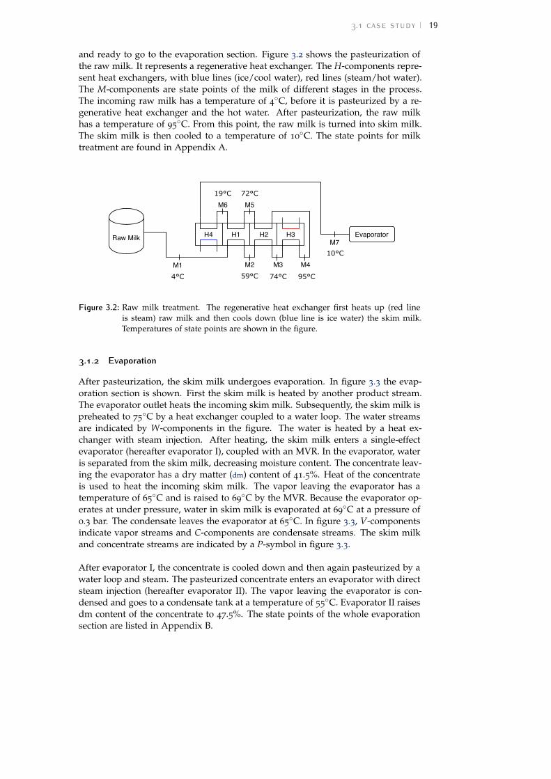
and ready to go to the evaporation section. Figure 3.2 shows the pasteurization ofthe raw milk. It represents a regenerative heat exchanger. The H-components repre-sent heat exchangers, with blue lines (ice/cool water), red lines (steam/hot water).The M-components are state points of the milk of different stages in the process.The incoming raw milk has a temperature of 4
C, before it is pasteurized by a re-generative heat exchanger and the hot water. After pasteurization, the raw milkhas a temperature of 95
C. From this point, the raw milk is turned into skim milk.The skim milk is then cooled to a temperature of 10
C. The state points for milktreatment are found in Appendix A.
EvaporatorH1 H2 H3H4
M1 M2 M3 M4
M5M6
M7Raw Milk
4°C 59°C 74°C 95°C
72°C19°C
10°C
Figure 3.2: Raw milk treatment. The regenerative heat exchanger first heats up (red lineis steam) raw milk and then cools down (blue line is ice water) the skim milk.Temperatures of state points are shown in the figure.
3.1.2 Evaporation
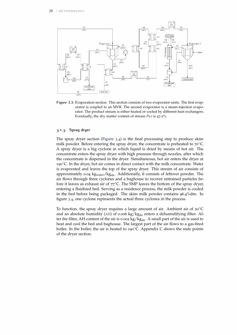
After pasteurization, the skim milk undergoes evaporation. In figure 3.3 the evap-oration section is shown. First the skim milk is heated by another product stream.The evaporator outlet heats the incoming skim milk. Subsequently, the skim milk ispreheated to 75
C by a heat exchanger coupled to a water loop. The water streamsare indicated by W-components in the figure. The water is heated by a heat ex-changer with steam injection. After heating, the skim milk enters a single-effectevaporator (hereafter evaporator I), coupled with an MVR. In the evaporator, wateris separated from the skim milk, decreasing moisture content. The concentrate leav-ing the evaporator has a dry matter (dm) content of 41.5%. Heat of the concentrateis used to heat the incoming skim milk. The vapor leaving the evaporator has atemperature of 65
C and is raised to 69C by the MVR. Because the evaporator op-
erates at under pressure, water in skim milk is evaporated at 69C at a pressure of
0.3 bar. The condensate leaves the evaporator at 65C. In figure 3.3, V-components
indicate vapor streams and C-components are condensate streams. The skim milkand concentrate streams are indicated by a P-symbol in figure 3.3.
After evaporator I, the concentrate is cooled down and then again pasteurized by awater loop and steam. The pasteurized concentrate enters an evaporator with directsteam injection (hereafter evaporator II). The vapor leaving the evaporator is con-densed and goes to a condensate tank at a temperature of 55
C. Evaporator II raisesdm content of the concentrate to 47.5%. The state points of the whole evaporationsection are listed in Appendix B.
20 methodology
Figure 3.3: Evaporation section. This section consists of two evaporator-units. The first evap-orator is coupled to an MVR. The second evaporator is a steam-injection evapo-rator. The product stream is either heated or cooled by different heat exchangers.Eventually, the dry matter content of stream P10 is 47.5%.
3.1.3 Spray dryer
The spray dryer section (Figure 3.4) is the final processing step to produce skimmilk powder. Before entering the spray dryer, the concentrate is preheated to 70
C.A spray dryer is a big cyclone in which liquid is dried by means of hot air. Theconcentrate enters the spray dryer with high pressure through nozzles, after whichthe concentrate is dispersed in the dryer. Simultaneous, hot air enters the dryer at190C. In the dryer, hot air comes in direct contact with the milk concentrate. Water
is evaporated and leaves the top of the spray dryer. This stream of air consists ofapproximately 0.04 kgwater/kgda. Additionally, it consists of leftover powder. Theair flows through three cyclones and a baghouse to recover entrained particles be-fore it leaves as exhaust air of 77
C. The SMP leaves the bottom of the spray dryer,entering a fluidized bed. Serving as a residence process, the milk powder is cooledin the bed before being packaged. The skim milk powder contains 96.4%dm. Infigure 3.4, one cyclone represents the actual three cyclones in the process.
To function, the spray dryer requires a large amount of air. Ambient air of 20C
and an absolute humidity (AH) of 0.006 kg/kgda enters a dehumidifying filter. Af-ter the filter, AH content of the air is 0.002 kg/kgda. A small part of the air is used toheat and cool the bed and baghouse. The largest part of the air flows to a gas-firedboiler. In the boiler, the air is heated to 190
C. Appendix C shows the state pointsof the dryer section.

3.2 pinch analysis 21
Spray Dryer
Heater
Fluidized Bed Dryer Product Out
Natural Gas
Air
A
A
A1A2
A4
A5 A6
A7
A8
A9
A10
A15
A11
A12
A13
A14
A16
A17
Exhaust Air
A3
N1
P11
P12
P13
P14
Product-in
Cyclone
FilterFilter powder
Baghouse
A19
P15
A18
Air toatmosphere
H15
H16
H17
H18
H14
P10
20°C
20°C
20°C
20°C
20°C
20°C
20°C
20°C
110°C
110°C
10°C
10°C
70°C
55°C
80°C
83°C
55°C
83°C
77°C
20°C
83°C
20°C
190°C
190°C 80°C
Figure 3.4: Spray drying section. This section includes a filter, heater, mixer, spray dryer,fluidized bed, cyclone, baghouse and multiple heat exchangers. The moisturecontent of the milk powder (P14 in the figure) is 3.6%.
3.2 pinch analysisAlready mentioned briefly in the literature review, the PM is a process integrationtechnique. It is a way to both visualize heat recovery options and calculate howmuch thermodynamically can be recovered. The following section will provide astep-by-step guide to do a pinch analysis.
3.2.1 Data extraction
The first step in the PM is to collect stream data. To obtain the heating and coolingrequirements for processes, the change in enthalpy must be calculated. The enthalpychange ∆H (kW) is determined by:
∆H = mh (3.1)
Where m (kg/s) is the mass flow rate and h (kJ/kg) is the specific enthalpy of aprocess stream. Enthalpy is always defined as a change, because a stream which ex-periences a reaction, either absorbs or accumulates energy. An important requisiteis that the mass flow rate stays constant. If this is not the case, the process streamis split and two reactions take place. The splitting and mixing of streams will bedescribed in section 3.2.4. For a constant mass flow rate, the formula for heating astream can be rewritten as:
∆H = mcp(Tt − Ts) (3.2)

22 methodology
The target temperature Tt (C) and supply temperature Ts (C) denote the differencein temperature change of a stream. The specific heat capacity cp (kJ/kgK) is amaterial-specific property. It is defined as the thermal energy requirement to raisethe temperature of 1 kg of material by 1 Kelvin. Although the specific heat capacityis temperature dependent, cp is assumed to be constant during reaction [42]. Forstreams which need to be cooled the target and supply temperature are switched inthe formula. When the previous equation is reformulated, it looks like:
∆H = CP∆T (3.3)
The heat capacity flowrate CP (kW/C) is the product of mass flow rate and specificheat capacity. Temperature difference ∆T (C) is the change in temperature beforeand after the reaction. This equation applies for heating and cooling processes. Itdoes not include evaporation and condensation processes. The evaporation andcondensation load are not calculated by temperature difference and heat capacityflowrate. Because a phase change occurs during evaporation and condensation atconstant temperature, only latent heat changes [43]. The heat load of evaporationand condensation is defined as:
∆H = m∆Hvap (3.4)
The heat of vaporization ∆H (kJ/kg) is the required energy to evaporate a liquid.
3.2.2 Stream selection
By identifying all the heat flows, a stream selection is made. Not all process streamsare included in the pinch analysis. Reason behind this logic lies in the definitionof a pinch analysis. Because heat recovery is the main purpose of this analysis,only streams which are eligible to be recovered, are included. Furthermore, whenrelevant streams are chosen, considerations must be made regarding intermediateprocess components. For example, how do you model a flow which is preheatedbefore an evaporator, then cooled by a heat exchanger and lastly heated by anotherheat exchanger?
There is no structured methodology for the selection of streams, but rather relies onthe considerations of the researcher. When there are intermediate components be-tween streams, i.e. (buffer)tanks, heat exchangers or other process units, the streamsshould be subdivided. There is a fine line in the subdivision of streams. Dividingstreams into too much little streams bares the risk of hiding potential recovery op-tions. To illustrate this, the following process flow is shown:
10°C 18°C 75°C
P1 P2 P3
Figure 3.5: Original process flow of preheating skim milk.
Figure 3.5 illustrates a basic process flow for preheating skim milk. The figureshows two process streams. In the first, skim milk is heated in a heat exchanger.The second stream is heated by another heat exchanger to its target temperature.When is decided to divide these streams in two separate streams, the temperaturesare too tightly specified. This implies that the temperature of P2, which is 18
C, isactually a target temperature which needs to be reached. In reality, this stream canbe any temperature according to the heat duty of the first heat exchanger. Dividingstreams in too many other streams increases complexity and produces constraintson recovery potential.

3.2 pinch analysis 23
To cope with the problem of subdividing streams, defining the soft and hard tem-perature of streams helps. Hard temperatures are invariable temperature, whichmust be met. On the other side, soft temperatures are variable temperatures. Softdata mean there is a window in which temperatures can vary without violating anyprocess standards.
When the soft and hard temperatures are defined, it becomes much easier to se-lect relevant streams for the pinch analysis. For instance, after defining soft andhard data for the process, it becomes clear how process streams must be modelledto be eligible for a pinch analysis. Recalling the example in figure 3.5, after definingsoft and hard data, this example must be modelled as one process stream. Thismeans that the supply temperature is 10
C and the target temperature is 75C. The
process stream for the pinch analysis now looks like figure 3.6. The heat duty ofthe two heat exchanger is now modelled as one heat exchanger with the same heatduty.
10°C 75°C
P1 P2
Figure 3.6: Data extraction for subdivided streams.
3.2.3 Intermediate and end-units
Another important consideration in selecting process streams, is the identificationof intermediate processes and end-units. For instance, how is a stream modelledthat passes a heat exchanger, vessel, evaporator or fluidized bed?
As the previous section showed, whether to include heat exchangers depends onsoft and hard temperatures. The same logic applies to vessels/tanks/evaporators.When both the composition, mass flow rate and the temperature of a stream, pass-ing a unit, stay constant, there is no reason to include the stream in a pinch analysis.However, a stream can be modelled if the stream temperature changes due to pass-ing a unit. When this is a hard temperature, the stream should be modelled in thepinch analysis.
When streams enter processes like evaporators, spray dryers and fluidized beds,the flow rate of the streams change. For instance, in an evaporator, the incomingstream is concentrated into a smaller flow. The same applies to a spray dryer andbed. A condition for a stream to be included in the pinch analysis is a constantflow rate. This means that streams passing process-units, in which the flow rate ischanged, are not included in a pinch analysis. An exemption exists when processstreams are mixed.
3.2.4 Mixing of streams
Another problem in stream selection is when streams are mixed. Especially mixedstreams with different temperatures may cause problems further in the analysis.When mixed streams are isothermal, the streams can be modelled as a single streamfor the pinch analysis. However, non-isothermal mixing can cause cross-pinch heattransfer. This is shown by the example in figure 3.7. Assume that the streamshave the same fluid composition. The mixer in the figure serves as a direct heatexchanger, reducing the temperature of the hot stream and increasing the tempera-ture of the cold stream. The hot air is being mixed with colder air to become air at80C. In terms of modelling for the pinch analysis, the process flow is considered as

24 methodology
one stream, i.e. the mixed stream A6. When the mixed stream is modelled as oneflow and the temperature is below pinch point, cooling capacity of the cold streamis gone. Stream A2 serves as a cold stream to cool down streams A5. When thepinch point is above 80
C, the pinch analysis shows that actually more cold utilityis required. In reality, no external cooling is required as stream A2 cools hot streamA5.
A5
A2
A6
190°C
20°C
80°C
Mixer
Figure 3.7: Original process flow diagram of mixed streams before entering spray dryer.
The right way to model mixed streams is isothermally. The multiple streamsbeing mixed, must have the same temperature. Figure 3.8 shows the right way formodelling mixed streams. As the target temperature of the stream is 80
C, the hotstream is being cooled to the target temperature and the cold stream is being heatedto the target temperature. In reality, the mixer serves as a heat exchanger. Now theprocess is seen as two streams because two imaginary heat exchangers bring thestreams to their target temperature.
A5b
A2b
A6
80°C
80°C
80°C
Mixer
A5a
A2a
190°C
20°C
Figure 3.8: Data extraction for mixed streams.
3.2.5 Composite curves
After all the data are extracted for the process streams, composite curves for hot andcold streams can be constructed. The composite curves are plotted on a temperature-enthalpy diagram. The hot and cold composite curves represent hot and coldstreams respectively. The first purpose of the curves is to graphically determinethe minimum external heating and cooling for a process. The second purpose is todefine the places for heat recovery by heat exchangers.
Figure 3.9 illustrates the method to plot the composite curves. Figure 3.9a repre-sents two hot streams which require cooling and figure 3.9b represents cold streams
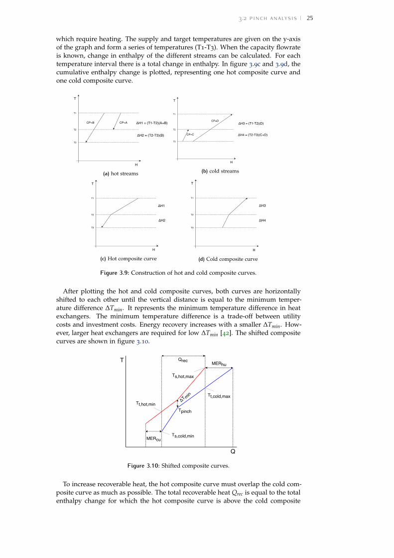
3.2 pinch analysis 25
which require heating. The supply and target temperatures are given on the y-axisof the graph and form a series of temperatures (T1-T3). When the capacity flowrateis known, change in enthalpy of the different streams can be calculated. For eachtemperature interval there is a total change in enthalpy. In figure 3.9c and 3.9d, thecumulative enthalpy change is plotted, representing one hot composite curve andone cold composite curve.
T
H
T1
T2
T3
CP=ACP=B ΔH1 = (T1-T2)(A+B)
ΔH2 = (T2-T3)(B)
(a) hot streams
T
H
T1
T2
T3
CP=D
CP=C
ΔH3 = (T1-T2)(D)
ΔH4 = (T2-T3)(C+D)
(b) cold streams
T
H
T1
T2
T3
ΔH1
ΔH2
(c) Hot composite curve
T
H
T1
T2
T3
ΔH3
ΔH4
(d) Cold composite curve
Figure 3.9: Construction of hot and cold composite curves.
After plotting the hot and cold composite curves, both curves are horizontallyshifted to each other until the vertical distance is equal to the minimum temper-ature difference ∆Tmin. It represents the minimum temperature difference in heatexchangers. The minimum temperature difference is a trade-off between utilitycosts and investment costs. Energy recovery increases with a smaller ∆Tmin. How-ever, larger heat exchangers are required for low ∆Tmin [42]. The shifted compositecurves are shown in figure 3.10.
Tpinch
MERhu
MERcu
Q
T
Ts,hot,max
Tt,hot,min
Ts,cold,min
Tt,cold,maxΔTmin
Qrec
Figure 3.10: Shifted composite curves.
To increase recoverable heat, the hot composite curve must overlap the cold com-posite curve as much as possible. The total recoverable heat Qrec is equal to the totalenthalpy change for which the hot composite curve is above the cold composite

26 methodology
curve. When placing heat exchangers, heat from the source (hot composite curve)can be transferred to the sink (cold composite curve). External heating and coolingis required where the composite curves do not overlap. The minimum energy re-quirement for cooling (MERcold) is necessary for the process below the pinch, whileminimum energy requirement for heating (MERhot) is necessary above the pinch. Thepoint where the temperature difference is smallest is called the pinch. The pinch isthe starting point for heat recovery as it represents a boundary. In section 3.2.6, therelevance of the pinch temperature will be explained.
An important rule for heat recovery applies to heat transfer. The rule states thatheat cannot be transferred across the pinch by a heat exchanger. Above the pinch,heat from the hot composite curve is transferred to the cold composite curve. Heat-ing is done by an external source (i.e. steam, hot air), making the area above thepinch a net heat sink. Below the pinch, the same logic is present. This area requiresexternal cooling duty (i.e. ice water), so heat flows out of the area. This area is a netheat source. When heat is transferred from the pinch, additional heat is requiredfor heating duty. Furthermore, because the area below the pinch is a heat source, itdoes not require external heating. Conversely, no external cooling is required abovethe pinch, as it is a heat sink [42].
Aside from defining minimum energy requirements, the composite curves showbetween which temperatures heat exchangers can recover heat. As discussed, thearea where the two curves overlap each other is eligible for recovery. Looking atthe hot composite curve, the supply temperature of hot streams can have a maxi-mum temperature of Ts,hot,max. The target temperature of hot streams can have aminimum temperature of Tt,hot,min. Following the same logic for the cold compos-ite curve, the minimum supply temperature for a cold stream is at Ts,cold,min. Themaximum target temperature for a cold stream is Tt,cold,max.
3.2.6 Grand Composite Curve
When the composite curves are plotted, the Grand Composite Curve (GCC) can beconstructed. Where the composite curves show two graphs for heat flows, the GCCshows the net heat flow in a single graph. The GCC is plotted by extracting the heatrequirement for cold streams from the heat available from hot streams for giventemperatures. The GCC is based on shifted temperatures instead of actual temper-atures. The reason behind this logic is that the GCC represents both hot and coldcomposite curves in a single curve. To modify temperatures, half of the minimumtemperature difference is added to cold stream temperatures and subtracted fromhot stream temperatures. A simple example of a GCC is shown in figure 3.11. Theheat requirement Qhu is the minimum heat flow which is needed by external utility.The heat requirement Qcu is the minimum cold utility which is required to cool hotstreams. The pinch temperature in the GCC is the point where the x-axis is zero.At this temperature, no external heating or cooling is required, as this is the pointwhere the hot and cold composite curves touch. The pinch temperature functionsas a boundary line, which divides the background process in two part; one partrequires external hot utility and one part which requires external cold utility.
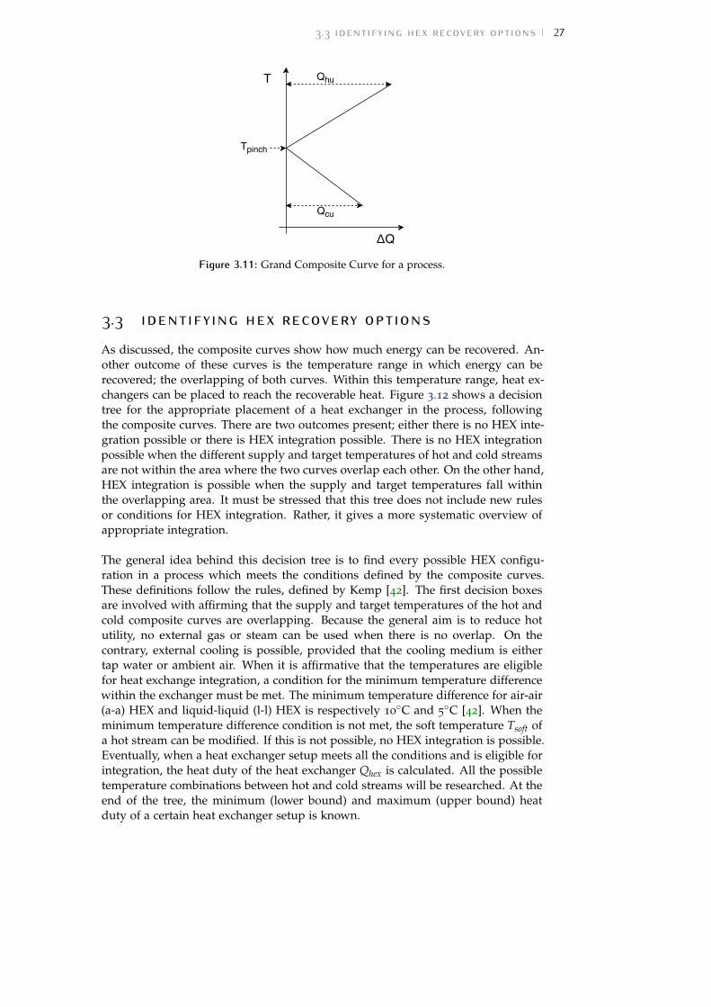
3.3 identifying hex recovery options 27
T
ΔQ
Qcu
Qhu
Tpinch
Figure 3.11: Grand Composite Curve for a process.
3.3 identifying hex recovery optionsAs discussed, the composite curves show how much energy can be recovered. An-other outcome of these curves is the temperature range in which energy can berecovered; the overlapping of both curves. Within this temperature range, heat ex-changers can be placed to reach the recoverable heat. Figure 3.12 shows a decisiontree for the appropriate placement of a heat exchanger in the process, followingthe composite curves. There are two outcomes present; either there is no HEX inte-gration possible or there is HEX integration possible. There is no HEX integrationpossible when the different supply and target temperatures of hot and cold streamsare not within the area where the two curves overlap each other. On the other hand,HEX integration is possible when the supply and target temperatures fall withinthe overlapping area. It must be stressed that this tree does not include new rulesor conditions for HEX integration. Rather, it gives a more systematic overview ofappropriate integration.
The general idea behind this decision tree is to find every possible HEX configu-ration in a process which meets the conditions defined by the composite curves.These definitions follow the rules, defined by Kemp [42]. The first decision boxesare involved with affirming that the supply and target temperatures of the hot andcold composite curves are overlapping. Because the general aim is to reduce hotutility, no external gas or steam can be used when there is no overlap. On thecontrary, external cooling is possible, provided that the cooling medium is eithertap water or ambient air. When it is affirmative that the temperatures are eligiblefor heat exchange integration, a condition for the minimum temperature differencewithin the exchanger must be met. The minimum temperature difference for air-air(a-a) HEX and liquid-liquid (l-l) HEX is respectively 10
C and 5C [42]. When the
minimum temperature difference condition is not met, the soft temperature Tsoft ofa hot stream can be modified. If this is not possible, no HEX integration is possible.Eventually, when a heat exchanger setup meets all the conditions and is eligible forintegration, the heat duty of the heat exchanger Qhex is calculated. All the possibletemperature combinations between hot and cold streams will be researched. At theend of the tree, the minimum (lower bound) and maximum (upper bound) heatduty of a certain heat exchanger setup is known.
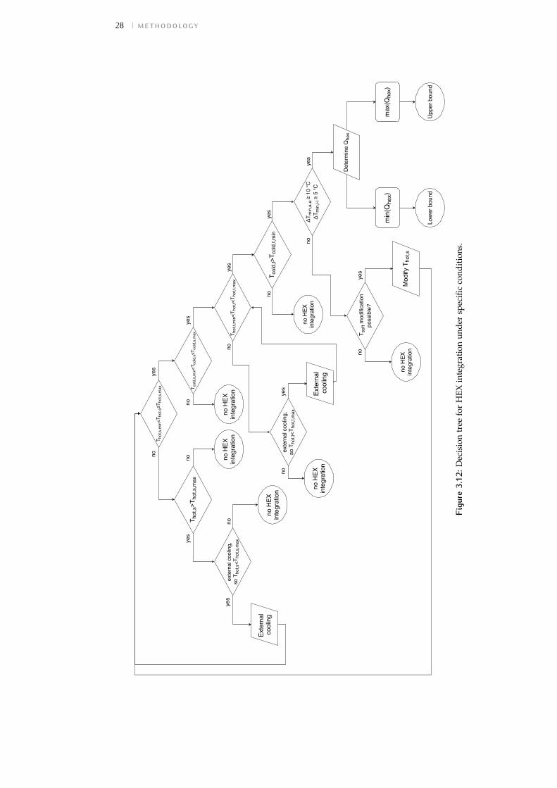
28 methodology
T hot,s,min<T
hot,s≤T
hot,s,max T c
old,s,min<T
cold,s≤T
cold,s,max T h
ot,t,min<T
hot,t<T
hot,t,max
T col
d,t>
T col
d,t,m
in
ΔT m
in,a-a
≥1
0 °C
ΔT m
in,l-l ≥5
°C
Det
erm
ine
Qhex
min(Q
hex)
max
(Qhe
x)
Low
er b
ound
Upp
er b
ound
no H
EXin
tegr
atio
n
T hot
,s>T
hot,s
,max
no
exte
rnal
coo
ling,
so Thot,s<T
hot,s,max
no H
EXin
tegr
atio
n
no
Exte
rnal
co
olin
g
no H
EXin
tegr
atio
n
yes
yes
yes
no
no
no H
EXin
tegr
atio
n
no
Tsoft
mod
ifica
tion
poss
ible
?
no H
EXin
tegr
atio
nM
odify
Tho
t,s
exte
rnal
coo
ling,
so Thot,t<T
hot,t,max
External
cooling
no H
EXin
tegr
atio
n
yes
yes
yes
yes
no
yes
no
no
no
yes
Figu
re3.
12:D
ecis
ion
tree
for
HEX
inte
grat
ion
unde
rsp
ecifi
cco
ndit
ions
.

3.4 graphical approach of heat pump integration 29
3.4 graphical approach of heat pump integrationThe GCC can be used to target energy requirements. Additionally, the curve helpsin the integration of different process units. For instance, using the GCC, appropri-ate placement of heat pumps can be identified. Kemp [42] introduced guidelines toplace heat pumps relative to the pinch temperature. Figure 3.13 shows an enthalpy-temperature graph, with a certain pinch temperature. Below the pinch temperature,there is heat surplus which requires cooling. This is seen in figure 3.13a. By placinga heat pump under the pinch temperature, heat (Qevap) is extracted and upgradedto a higher temperature (Qcond+Wel), by work input (Wel). The heat pump serves asa heater, while the surplus needs to cool down. Eventually, the system produceswaste heat (Qcu-Wel) to the environment. On 3.13b, the heat pump is placed abovethe pinch temperature. This area requires heating, as there is a heat deficit. Theheat pump serves as an electrical heater to the process, extracting low tempera-ture heat (Qevap) from the process and transferring it back to high temperature heat(Qcond+Wel).
Pinch Temp.
T
Q
Heat Surplus
Heat Deficit
Wel
Qcond+Wel
Qevap
Qcu + Wel
Qhu
(a) Inappropriate placement of an VCHP underPinch temperature.
Pinch Temp.
T
Q
Heat Surplus
Heat Deficit
Wel
Qcond+Wel
Qevap
Qcu
Qhu+ Wel
(b) Inappropriate placement of an VCHP above thePinch temperature.
Pinch Temp.
T
Q
Heat Surplus
Heat Deficit
Wel
Qcond+Wel
Qevap
Qcu-Qevap
Qhu-(Qcond+ Wel)
(c) Appropriate placement of a heat pump across thepinch temperature.
Figure 3.13: Placing an VCHP in the process using the GCC.
Net energy savings are only accomplished when a heat pump is placed acrossthe pinch temperature [42]. Figure 3.13c shows the appropriate placement of a heatpump. At the source, heat is in excess, while the sink requires heat. The heat pumptransfers heat surplus (Qevap) from the source across the pinch temperature to theheat sink (Qcond+Wel). A heat pump results in a decline of heating ((Qhu-(Qcond+Wel))and cooling (Qcu-Qevap).

30 methodology
Figure 3.14 shows the approach to integrate a heat pump system in a process, us-ing the GCC. The figure represents the integration of a heat pump in an exampleGCC. As shown in figure 3.14, the net heat flow at the pinch temperature is zero.The pinch is the dividing line that separates the streams which need cooling andheating. The task of a heat pump is to connect those two areas, i.e. transfer heatfrom lower temperature heat sources to higher temperature heat sinks. Because thepinch temperature is Tpinch, the heat source should be below Tpinch. On the contrary,the temperature of the heat sink should be higher than Tpinch. The heat below thepinch is used in the evaporator to vaporize a working fluid. Because hot streamsrelease heat to the fluid, external cooling is decreased. This heat is released to theheat sink in the condenser of the heat pump. This reduces external heating. Whatthe heat pump does, is transferring heat to an area where heat is required. The netheat flow at the pinch is zero. This point determines from which temperature theheat pump uses heat. The red line in the figure represents the evaporation heat.This must be as close to the pinch as possible. Closer to the pinch means that thetemperature lift is smaller. A smaller temperature lift results in a higher COP. Bymeans of work input, the heat pump releases condensation heat to a heat sink abovethe pinch. The amount of heat released to a sink is equal to the evaporation heatand the work input combined.
ΔQ
evaporation
condensation
Heat
Heat pump
work input
Tpinch
Figure 3.14: Heat pump integration using the GCC.
What can be learned from the GCC is whether it is viable to integrate a heatpump. A requisite for appropriate heat pump placement is the existence of a sharpnose at the pinch temperature in the GCC. When this is the case, the temperaturelift is also small. A smaller temperature lift means less work input and a higherCOP. When the nose is more convex, the temperature lift must be higher to releasethe same amount of heat to a sink. Figure 3.15 shows a graphical example of asharp (3.15a) and convex GCC nose (3.15b).
(a) Sharp nose integration. (b) Convex nose integration.
Figure 3.15: GGC’s with heat pump integration.

3.5 identifying hp heat recovery options 31
3.5 identifying hp heat recovery optionsLike the decision tree for placing a HEX in the process, figure 3.16 shows a decisiontree for the appropriate placement of an HP in the process. This decision tree isbased on the conditions of the GCC for appropriately placing an HP [42]. Thus,heat is extracted from below the pinch temperature and released above the pinchtemperature. Again, this tree illustrates a systematic overview of HP integration,composed of existing conditions [42].
The condition for placing an HP is that the heat source supply temperature Tsource,s isbelow the pinch temperature. Furthermore, the heat sink supply temperature Tsink,smust be above the pinch temperature. Another condition, regardless of the pinchanalysis, is defined by the minimum heat source target temperature Tsource,t,min. TheTsource,t,min is a process-bounded minimum temperature. An examples of such atemperature is the water discharge temperature into the environment. Additionally,the heat sink target requirement temperature Tsink,t,req is a process-bounded temper-ature. The requirement temperature is identical to a hard temperature. In order tooperate the process, hard temperatures must be met. In section 4.4, the differenttemperatures will be defined. Another condition is the minimum COP of a heatpump. In this research the COP of an HP must be at least 5 [44].
Similar to the HEX decision tree, the general idea behind this decision tree is tofind every possible HP configuration in a process that meets the conditions of theGCC. Eventually, when an HP setup meets all the conditions and is eligible for inte-gration, the condensation heat released to the heat sink Qcond is calculated. All thepossible setups, i.e. heat source and heat sink temperatures, will be researched. Atthe end, the minimum (lower bound) and maximum (upper bound) condensationheat of a certain HP setup are known.
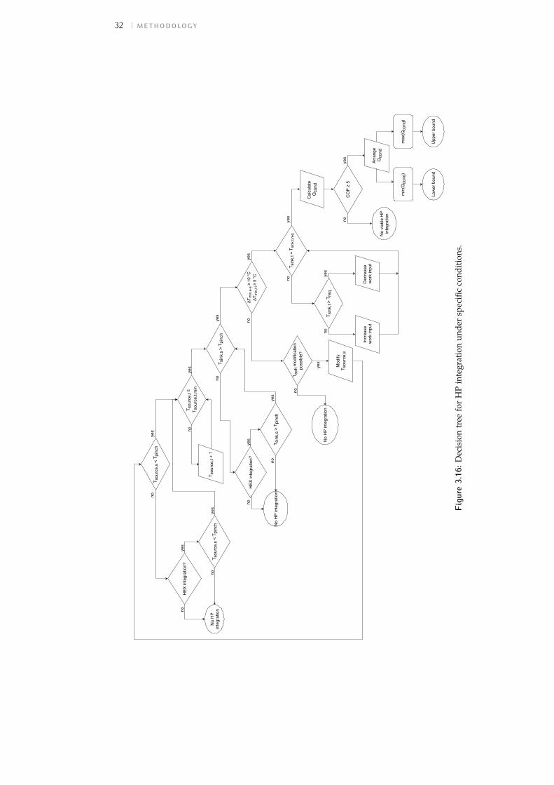
32 methodology
T sou
rce,
s <
T pin
ch
T sou
rce,
t ≥
T source,t,m
in
T sin
k,s
>T pinch
ΔT m
in,a-a ≥10 °C
ΔT m
in,l-l ≥5 °C
yes
yes
yes
yes
HEX
inte
grat
ion?
no
No
HP
inte
grat
ionno
yes
T sou
rce,
s <
T pin
chye
sno
T sou
rce,
t + 1
no
HEX
inte
grat
ion?
no
No
HP
inte
grat
ion
no
T sin
k,s
> T p
inch
yes
yes
no
Cal
cula
te
Qco
nd
Low
er b
ound
max
(Qco
nd)
Upp
er b
ound
T sin
k,t =
Tsink,t,req
CO
P ≥5
Arra
nge
Qco
nd
Tso
ft m
odifi
catio
npo
ssib
le?
No
HP
inte
grat
ion
no
Mod
ifyT s
ourc
e,s
yes
yes
yes
T sin
k,t >
Tre
q
no
Dec
reas
e w
ork
inpu
tIn
crea
se w
ork
inpu
t
yes
no
no
No
viab
le H
Pin
tegr
atio
n
min
(Qco
nd)
no
Figu
re3.
16:D
ecis
ion
tree
for
HP
inte
grat
ion
unde
rsp
ecifi
cco
ndit
ions
.

3.6 integration of zeolite wheel 33
3.6 integration of zeolite wheelSo far, heat sources and sinks can be identified using the small composite curvesand the GCC. The use of one of these curves to identify the placement of a zeoliteis unnecessary. A zeolite wheel is used to dehumidify air. So, there are two placesin the process where a zeolite wheel can be useful; at the air inlet and the air outletof a process. In the case study, there is one place where air comes in. This is theair inlet of the air heater in the spray drying section. At this point, there is alreadya sorption unit dehumidifying ambient air. The only point where air exits the casestudy, is the exhaust of the spray dryer. Therefore, the placement of a zeolite wheelat the spray dryer exhaust will be researched.
3.7 environmental analysisTo assess the environmental performance of different technologies, both the directand indirect carbon emissions are considered. Therefore, the total annual emissionsEtotal (kg CO2-e/yr) for a technology configuration j are:
Etotal,j = Eindirect,j − Edirect,j (3.5)
The indirect emissions Eindirect (kg CO2-e/yr) will be the emissions associated withthe manufacturing of technology configuration j. The direct emissions Edirect (kgCO2-e/yr) are the annual emissions saved by configuration j. The indirect emissionsEindirect,j are calculated by:
Eindirect,j = (Ere f
nj
Dj
Dre f)σ (3.6)
Where Eref (kg CO2-e) is the reference emission, n is the lifetime (years), D is adimension, Dref is the dimension from a reference and σ (-) is a scaling factor. Theunits of the dimensions D and Dref are technology specific. The direct emissionsEdirect,j are calculated by:
Edirect,j = ∑j
Qu,j Ie (3.7)
The direct emissions are calculated by the utility requirement Qu,j (kWh/yr) ofutility u and the carbon intensity I (kg CO2-e/kWh) of energy carrier e. Note thatthe electricity demand is a positive value and the heat savings are a negative value.
3.8 economic analysisTo fully understand the effect of different technologies, the economic savings oftechnology configurations are estimated. The total annual costs (TAC) (e/yr) aredetermined by:
TAC = ∑j
EACj + ∑j
Cu,j −∑j
EjPcarbon (3.8)
The total costs are dependent on the equivalent annual costs (EAC) (e/yr) for pro-cess j, the annual cost savings C (e/yr) for utility u and the carbon savings E (tCO2-e/yr) and price of carbon Pcarbon (e/tCO2-e). Note that the amount of carbon savedis an opportunity cost in the equation. The EAC is determined by:
EAC =∑j Cinv,jLFi
1− (1 + i)−n (3.9)

34 methodology
It is based on the capital investment Cinv (e) of process j, the Lang Factor (LF)(-), the discount rate i (%) and the lifetime of the technology n (years). The LFis a factor to include manufacturing and installing equipment. Furthermore, thecapital investments are based on many factors and are not similar. Therefore, twomethods are used to define capital investments. The investment for the zeolite Cinv,zis determined by the cost of a reference [34], so:
Cinv,z = Cre fDz
Dre f(3.10)
Where Cref (e) is the capital investment of the zeolite wheel in a reference, Dz(kgwater/s) is the dimension of the zeolite in this study and Dref (kgwater/s) is thedimension of the zeolite in the reference study.
The capital investments of a heat exchanger Cinv,hex are determined by the Hallmethod [45] for stainless steel shell-tube heat exchangers:
Cinv,hex = 8500 + 409A0.85 (3.11)
The total investment costs for a heat pump Cinv,hp are:
Cinv,hp = 2517W0.7849 + 2Cinv,hex (3.12)
The first part of the equation determines the investment cost of a screw compressor[46]. The variable W (kW) is the amount of work input of the compressor. Thesecond part of the equation represents the evaporator and condenser in the heatpump cycle. Investments for pipelines and expansion valves are neglected.
3.9 data
3.9.1 Mass flow rate and temperature
Process & Instrumentation Diagrams (P&ID) provide data to construct a process flowsheet. The P&ID’s are important for the origin and destination of pipelines, heatexchangers and unit processes, like evaporators and the spray dryer.
First, mass flow rate and temperature data are collected from a SCADA-system.Following the identification number of certain sensors, mass flow and temperaturecan be retrieved. Specific flows are metered, collected and visualized in a chart.Often such a chart is similar to figure 3.17:
Mas
s fl
ow
rat
e/te
mp
erat
ure
Time
CIP
Shutdown
Startup
CIP
Run
Figure 3.17: Schematic operations curve.
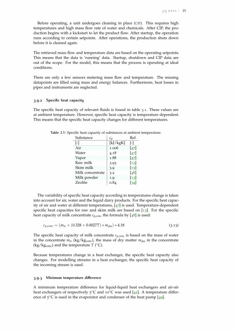
3.9 data 35
Before operating, a unit undergoes cleaning in place (CIP). This requires hightemperatures and high mass flow rate of water and chemicals. After CIP, the pro-duction begins with a kickstart to let the product flow. After startup, the operationruns according to certain setpoints. After operations, the production shuts downbefore it is cleaned again.
The retrieved mass flow and temperature data are based on the operating setpoints.This means that the data is ‘running’ data. Startup, shutdown and CIP data areout of the scope. For the model, this means that the process is operating at idealconditions.
There are only a few sensors metering mass flow and temperature. The missingdatapoints are filled using mass and energy balances. Furthermore, heat losses inpipes and instruments are neglected.
3.9.2 Specific heat capacity
The specific heat capacity of relevant fluids is found in table 3.1. These values areat ambient temperature. However, specific heat capacity is temperature dependent.This means that the specific heat capacity changes for different temperatures.
Table 3.1: Specific heat capacity of substances at ambient temperature.Substance cp Ref.[-] [kJ/kgK] [-]Air 1.006 [47]Water 4.18 [47]Vapor 1.88 [47]Raw milk 3.93 [13]Skim milk 3.9 [13]Milk concentrate 3.2 [48]Milk powder 1.9 [13]Zeolite 0.84 [34]
The variability of specific heat capacity according to temperatures change is takeninto account for air, water and the liquid dairy products. For the specific heat capac-ity of air and water at different temperatures, [47] is used. Temperature-dependentspecific heat capacities for raw and skim milk are based on [13]. For the specificheat capacity of milk concentrate cp,conc the formula by [48] is used:
cp,conc = (mw + (0.328 + 0.0027T) ∗mdm) ∗ 4.18 (3.13)
The specific heat capacity of milk concentrate cp,conc is based on the mass of waterin the concentrate mw (kg/kgconc), the mass of dry matter mdm in the concentrate(kg/kgconc) and the temperature T (C).
Because temperatures change in a heat exchanger, the specific heat capacity alsochanges. For modelling streams in a heat exchanger, the specific heat capacity ofthe incoming stream is used.
3.9.3 Minimum temperature difference
A minimum temperature difference for liquid-liquid heat exchangers and air-airheat exchangers of respectively 5
C and 10C was used [42]. A temperature differ-
ence of 5C is used in the evaporator and condenser of the heat pump [49].
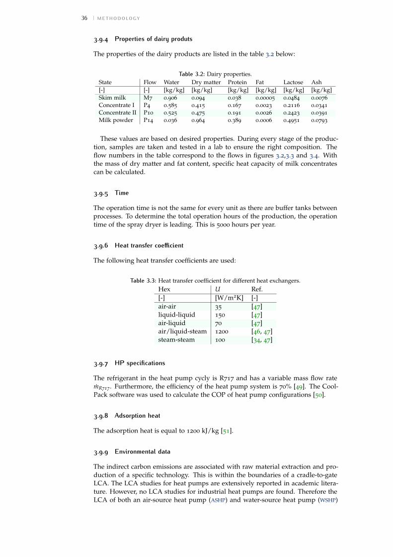
36 methodology
3.9.4 Properties of dairy produts
The properties of the dairy products are listed in the table 3.2 below:
Table 3.2: Dairy properties.State Flow Water Dry matter Protein Fat Lactose Ash[-] [-] [kg/kg] [kg/kg] [kg/kg] [kg/kg] [kg/kg] [kg/kg]Skim milk M7 0.906 0.094 0.038 0.00005 0.0484 0.0076
Concentrate I P4 0.585 0.415 0.167 0.0023 0.2116 0.0341
Concentrate II P10 0.525 0.475 0.191 0.0026 0.2423 0.0391
Milk powder P14 0.036 0.964 0.389 0.0006 0.4951 0.0793
These values are based on desired properties. During every stage of the produc-tion, samples are taken and tested in a lab to ensure the right composition. Theflow numbers in the table correspond to the flows in figures 3.2,3.3 and 3.4. Withthe mass of dry matter and fat content, specific heat capacity of milk concentratescan be calculated.
3.9.5 Time
The operation time is not the same for every unit as there are buffer tanks betweenprocesses. To determine the total operation hours of the production, the operationtime of the spray dryer is leading. This is 5000 hours per year.
3.9.6 Heat transfer coefficient
The following heat transfer coefficients are used:
Table 3.3: Heat transfer coefficient for different heat exchangers.Hex U Ref.[-] [W/m2K] [-]air-air 35 [47]liquid-liquid 150 [47]air-liquid 70 [47]air/liquid-steam 1200 [46, 47]steam-steam 100 [34, 47]
3.9.7 HP specifications
The refrigerant in the heat pump cycly is R717 and has a variable mass flow ratemR717. Furthermore, the efficiency of the heat pump system is 70% [49]. The Cool-Pack software was used to calculate the COP of heat pump configurations [50].
3.9.8 Adsorption heat
The adsorption heat is equal to 1200 kJ/kg [51].
3.9.9 Environmental data
The indirect carbon emissions are associated with raw material extraction and pro-duction of a specific technology. This is within the boundaries of a cradle-to-gateLCA. The LCA studies for heat pumps are extensively reported in academic litera-ture. However, no LCA studies for industrial heat pumps are found. Therefore theLCA of both an air-source heat pump (ASHP) and water-source heat pump (WSHP)

3.9 data 37
are used as a reference [52]. With regard to the indirect carbon emissions of heatexchangers, one cradle-to-grave LCA is found [53]. The emissions for extractionand manufacturing are used as a reference.
Unfortunately, there are no LCA studies regarding zeolite/desiccant wheels. There-fore, another method for calculating the indirect carbon emissions for the desiccantwheel is chosen. The material requirements of a specific dimension are used as baseto calculate the indirect carbon emissions. Table 3.4 shows the material requirementfor a zeolite wheel, together with the carbon intensity of the specific material.
Table 3.4: Mass composition of a zeolite wheel. The material requirement of the wheel isfrom [54].
Material Mass Eindirect Ref.[-] [kg] [kg CO2-eq/kg] [-]Aluminium 190 3.94 [55]Zeolite 310 2.523 [56]Steel 120 2.459 [57]Rubber 2 0.7 [58]
The indirect carbon emissions of the different materials are retrieved from vari-ous LCA studies. The emissions are associated with raw material extraction andprocessing to a final product. This means that these carbon emission values do notinclude the manufacturing of an actual zeolite wheel. Additional energy is requiredto process and assemble the materials into a wheel. Therefore, a scaling factor σ isintroduced. The value is arbitrarily chosen.
The environmental input variables for the different technologies are shown in ta-ble 3.5:
Table 3.5: Environmental data for heat recovery technologies.Technology Eref Dref n σ Ref.[-] [kg CO2-e] [-] [years] [-] [-]HEX 32000 274 m2
20 1.5 [53]ASHP 0.014 1 kWht 20 1 [52]WSHH 0.009 1 kWht 20 1 [52]ZW 1830 0.012 kgwater/s 5 2.5 [54, 55, 56, 57, 58]
The reference dimensions for the heat exchanger, heat pumps and zeolite wheelare respectively HEX area, condensation heat and MRC. The chosen scaling factorsare based on the boundary of the relevant LCA studies.
The carbon intensity per energy source is listed in table 3.6. The carbon inten-sity varies for different studies as researchers set different boundaries. For example,a distinction can be made between carbon intensity of downstream, upstream andconsumption processes of natural gas and/or electricity. The data in table 3.6 fornatural gas are based on various studies and an appropriate deviation is chosen[13, 59]. Regarding the energy mix for the generation of electricity; in the futurethe case study will consume electricity generated from renewable sources from af-filiated farms. Without considering indirect carbon emissions, the carbon intensityof electricity is then zero. However, following different sources, when gas or coalis used for the generation of electricity, the carbon intensity may reach 0.6 kg/kWh[60, 61]. Therefore, a range of 0 to 0.6 kg/kWh for electricity generation is chosen.
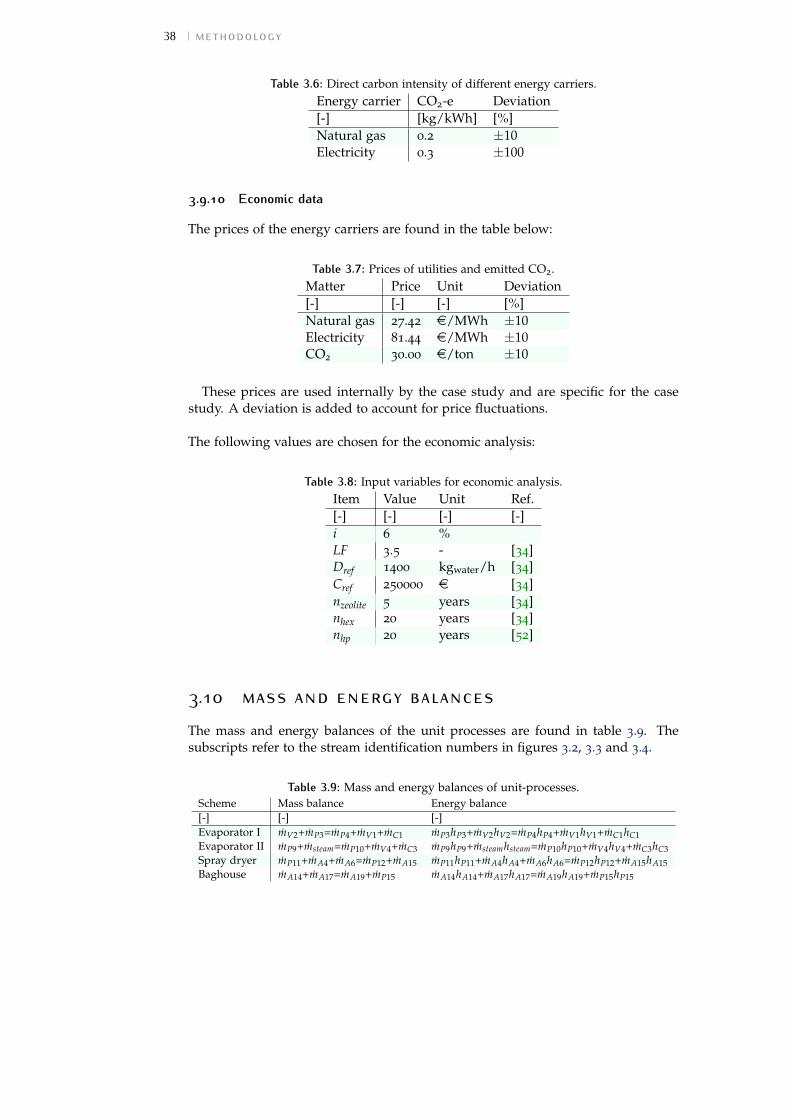
38 methodology
Table 3.6: Direct carbon intensity of different energy carriers.Energy carrier CO2-e Deviation[-] [kg/kWh] [%]Natural gas 0.2 ±10Electricity 0.3 ±100
3.9.10 Economic data
The prices of the energy carriers are found in the table below:
Table 3.7: Prices of utilities and emitted CO2.Matter Price Unit Deviation[-] [-] [-] [%]Natural gas 27.42 e/MWh ±10Electricity 81.44 e/MWh ±10CO2 30.00 e/ton ±10
These prices are used internally by the case study and are specific for the casestudy. A deviation is added to account for price fluctuations.
The following values are chosen for the economic analysis:
Table 3.8: Input variables for economic analysis.Item Value Unit Ref.[-] [-] [-] [-]i 6 %LF 3.5 - [34]Dref 1400 kgwater/h [34]Cref 250000 e [34]nzeolite 5 years [34]nhex 20 years [34]nhp 20 years [52]
3.10 mass and energy balancesThe mass and energy balances of the unit processes are found in table 3.9. Thesubscripts refer to the stream identification numbers in figures 3.2, 3.3 and 3.4.
Table 3.9: Mass and energy balances of unit-processes.Scheme Mass balance Energy balance[-] [-] [-]Evaporator I mV2+mP3=mP4+mV1+mC1 mP3hP3+mV2hV2=mP4hP4+mV1hV1+mC1hC1Evaporator II mP9+msteam=mP10+mV4+mC3 mP9hP9+msteamhsteam=mP10hP10+mV4hV4+mC3hC3Spray dryer mP11+mA4+mA6=mP12+mA15 mP11hP11+mA4hA4+mA6hA6=mP12hP12+mA15hA15Baghouse mA14+mA17=mA19+mP15 mA14hA14+mA17hA17=mA19hA19+mP15hP15
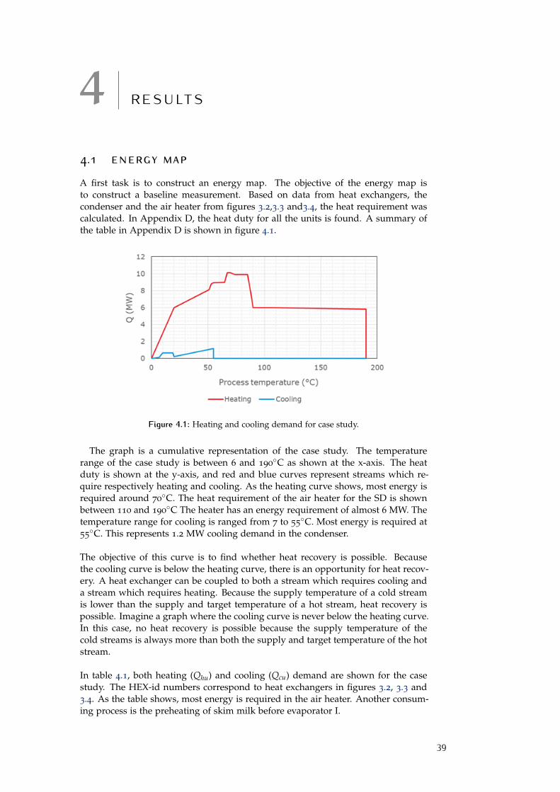
4 R E S U LT S
4.1 energy mapA first task is to construct an energy map. The objective of the energy map isto construct a baseline measurement. Based on data from heat exchangers, thecondenser and the air heater from figures 3.2,3.3 and3.4, the heat requirement wascalculated. In Appendix D, the heat duty for all the units is found. A summary ofthe table in Appendix D is shown in figure 4.1.
Figure 4.1: Heating and cooling demand for case study.
The graph is a cumulative representation of the case study. The temperaturerange of the case study is between 6 and 190
C as shown at the x-axis. The heatduty is shown at the y-axis, and red and blue curves represent streams which re-quire respectively heating and cooling. As the heating curve shows, most energy isrequired around 70
C. The heat requirement of the air heater for the SD is shownbetween 110 and 190
C The heater has an energy requirement of almost 6 MW. Thetemperature range for cooling is ranged from 7 to 55
C. Most energy is required at55C. This represents 1.2 MW cooling demand in the condenser.
The objective of this curve is to find whether heat recovery is possible. Becausethe cooling curve is below the heating curve, there is an opportunity for heat recov-ery. A heat exchanger can be coupled to both a stream which requires cooling anda stream which requires heating. Because the supply temperature of a cold streamis lower than the supply and target temperature of a hot stream, heat recovery ispossible. Imagine a graph where the cooling curve is never below the heating curve.In this case, no heat recovery is possible because the supply temperature of thecold streams is always more than both the supply and target temperature of the hotstream.
In table 4.1, both heating (Qhu) and cooling (Qcu) demand are shown for the casestudy. The HEX-id numbers correspond to heat exchangers in figures 3.2, 3.3 and3.4. As the table shows, most energy is required in the air heater. Another consum-ing process is the preheating of skim milk before evaporator I.
39

40 results
Table 4.1: Overview of utility consuming units.Section HEX-id Qhu HEX-id Qcu[-] [-] [kW] [-] [kW]Milk treatment H3 1087 H4 452
Evaporation I preheating H7 2133 - -Evaporation II preheating H12 682 H9 146
H13 61 - -Spray dryer preheating H14 151 - -Air heater Heater 5827 - -FB & BH H15 98 H17 28
H16 50 H18 28
4.2 process flow sheet for pinch analysisBefore selecting relevant streams, a process flow diagram is drawn. Figure 4.2shows this process flow diagram. From the diagram, the streams can be selectedwhich are relevant for a pinch analysis. The numbers at the streams in the figurecorrespond to supply and target temperatures. The H- and C-components are re-spectively heaters and coolers. The heat duty of the heat exchangers is shown nearthe exchangers. The Cond.-component is the condenser for evaporator II, in whichvapor from the evaporator is condensed. The flow diagram is based on figures 3.2,3.3 and 3.4. Note that the mixed streams A2 and A5 in figure 4.2 are individuallyheated or cooled so isothermal mixing take place. This is done by heat exchangersH6 and C5.
As stated before, only streams which require heating/cooling are considered in thepinch analysis. From the process flow sheet, stream data can be extracted. Table 4.2shows the process stream data. Note that evaporation is excluded from the pinchanalysis. The streams are divided in one of the three sections: milk treatment (MT),evaporation (EV) and spray drying. The heat exchanger numbers (HEX-id) in thetable correspond to the numbers in the process flow sheet. The supply and targettemperatures Ts and Tt are extracted from the sheet. The heat capacity flow rate CPis based on the mass flow rate and specific heat capacity of a flow. These parameterscan be found in Appendix A-C. When knowing the temperature difference and theheat capacity flow rate, the heat duty Q of the heat exchanger is calculated. Thetarget temperatures with an asterisk (*) are based on soft data.
The condenser was modelled different from the heat exchangers. In the heat ex-changers, only sensible heat is transferred. Because there is a phase-change in thecondenser, the latent heat duty is relevant only. Vapor at 55
C is condensed andleaves the condenser at 55
C. Thus, no sensible heat is released. The heat of vapor-ization of heat of water at 55
C is approximately 2370 kJ/kg. With a flow of 0.8kg/s, the latent heat duty of the condenser is 1185 kW.
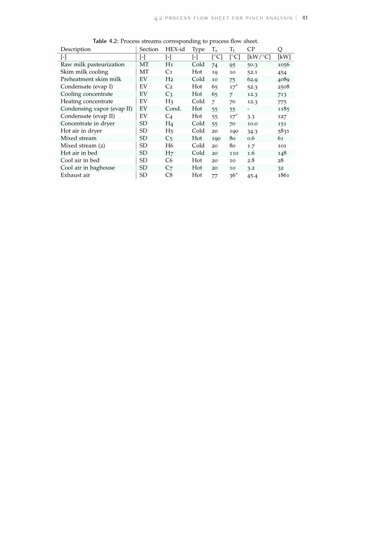
4.2 process flow sheet for pinch analysis 41
Table 4.2: Process streams corresponding to process flow sheet.Description Section HEX-id Type Ts Tt CP Q[-] [-] [-] [-] [C] [C] [kW/C] [kW]Raw milk pasteurization MT H1 Cold 74 95 50.3 1056
Skim milk cooling MT C1 Hot 19 10 52.1 454
Preheatment skim milk EV H2 Cold 10 75 62.9 4089
Condensate (evap I) EV C2 Hot 65 17∗
52.3 2508
Cooling concentrate EV C3 Hot 65 7 12.3 713
Heating concentrate EV H3 Cold 7 70 12.3 775
Condensing vapor (evap II) EV Cond. Hot 55 55 - 1185
Condensate (evap II) EV C4 Hot 55 17∗
3.3 127
Concentrate in dryer SD H4 Cold 55 70 10.0 151
Hot air in dryer SD H5 Cold 20 190 34.3 5831
Mixed stream SD C5 Hot 190 80 0.6 61
Mixed stream (2) SD H6 Cold 20 80 1.7 101
Hot air in bed SD H7 Cold 20 110 1.6 148
Cool air in bed SD C6 Hot 20 10 2.8 28
Cool air in baghouse SD C7 Hot 20 10 3.2 32
Exhaust air SD C8 Hot 77 36∗
45.4 1861
42 results
Spra
y dr
yer
Flui
dize
d be
d
Cyclone
202020
2019
019
0
190
80
80
80
55 70
110
10
2010
8020
2077
5583
83
83
Tank
Tank
70
657
65 17
7510
459
7495
72
19
Atm
osph
ere
1056
kW
H1
C1
H2
454
kW40
89 k
W C2
2508
kW
C3 71
3 kW
775
kWH
3
17
127
kWC
4
H4
151
kW
H5
C5
H6
5831
kW
H7 14
8 kW
28 k
WC
6
32 k
WC
7
36
C8
1856
kW
101
kW
61 k
WCon
d.
55 55
1185
kW
Baghouse
Atm
osph
ere
Atm
osph
ere Pack
agin
g
Pack
agin
g
Milk
rece
ptio
n
Evap
orat
orEv
apor
ator
Figu
re4.
2:Pr
oces
sflo
wsh
eet.

4.2 process flow sheet for pinch analysis 43
With the exception of the temperatures with an asterisk, all temperatures in thetable are hard temperatures. This means that in order to produce milk powderaccording to its process standards, hard temperatures must be met. The tempera-tures with an asterisk are soft temperatures. These temperature can vary withoutdeteriorating the process quality. The streams based on soft target temperatures arethe condensate flows from evaporator I and II and the exhaust from the spray dryer.
In reality, the two condensate streams are being discharged at respectively 37 and55C as shown by streams C2 and C4 in figure 4.2. After leaving evaporator I at
65C, some heat of the condensate is recovered by incoming skim milk. Eventually
the condensate leaves the process at 37C. Condensate from evaporator II leaves the
process at 55C, without heat recovery. To know how much heat can be recovered
from the condensate, the target temperatures of both streams are different from theactual temperature at which they are discharged. A suitable target temperaturecould be the coldest supply temperature plus the minimum temperature differencein the pinch analysis. This would result in a target temperature of 17
C. At thistarget temperature, condensate could hypothetically be integrated with the coldestsupply temperature by a heat exchanger.
Another target temperature based on soft data is the exhaust of the spray dryer.The exhaust has a temperature of 77
C. This stream is not recovered yet. Processengineers are restrained in recovering the exhaust stream because of milk powderparticles in the air stream. When the air drops in temperature, the flow is closer tosaturation with vapor. When the stream is completely saturated, air is at its dewpoint. When this happens, entrained particles in the exhaust become slurry andsticky. This means that when the exhaust is recovered close to its dew point, stickyair could affect the performance of a heat exchanger. Sticky milk powder can stickto the tube-wall of a heat exchanger. In the pinch analysis, the dew point is takenas target temperature for the exhaust to see what the maximum recoverable heat isbefore saturation. However, in reality, recovering exhaust heat until dew point willbe less favorable.
Figure 4.3 shows a Mollier chart of the exhaust air from the spray dryer. Theambient air has a temperature of 20
C with an AH of 0.006 kg/kgda (Tamb). Af-ter dehumidifying and heating, the inlet air is 190
C and the AH is 0.002 kg/kgda(Texh). As the air takes up moisture from the concentrate, the exhaust air has an AHof 0.04 kg/kgda at 77
C (Texh). At this AH level, the dew point is the point wherethe air is saturated (at 100% relative humidity (RH)). From the graph, the RH ofthe exhaust is around 10%. The dew point (Tdp) is at 36
C. When the exhaust airis approaching dew point it is saturated with vapor. The target temperature of thespray dryer exhaust will be equal to the dew point, i.e. 36
C.

44 results
Tamb Tin
TexhTDP
Heater
SD
0
0,02
0,04
0,06
0,08
0,1
0,12
0 50 100 150 200
AH
(kg
w/k
g da)
Temperature (°C)
Figure 4.3: Mollier chart of SD exhaust. The temperature of ambient air is heated to theSD inlet temperature (indicated by ‘Heater’ in the figure). In the SD, the airtemperature is decreased to 77
C (indicated by ‘SD’).
4.3 composite curves
The hot and cold composite curves for the process have been drawn according to thedata from table 4.2. Figure 4.4 shows the curves. The red and blue curve representrespectively the hot and cold streams. The pinch temperature Tpinch is 50
C. Atthat temperature, the process is split into an area which requires cooling and anarea which requires heating. The total external hot utility demand Qhu is 6.8 MW.The total cold utility demand Qcu is 1.7 MW. This means that the total recoverableheat Qrec is 5.3 MW. Important to note, the composite curves serve as a referencecase. This means that proposed configurations are compared against the resultsof the pinch analysis. The outcomes of a new HEX configuration are comparedagainst Qrec. This means that 5.3 MW serves as a base case to compare with HEXconfigurations. With regard to HP and zeolite configurations, the Qhu, i.e. 6.8 MWserves as reference.
32 °C
77 °C
60 °C
Qhu = 6.8 MW
Qcu = 1.7 MW
Tpinch = 50°C
Qrec = 5.3 MW
0
20
40
60
80
100
120
140
160
180
200
0 2 4 6 8 10 12 14
T (°C)
Q (MW)
Hot composite curve Cold composite curve
Figure 4.4: Composite curves.

4.3 composite curves 45
Starting with the hot composite curve; it begins at 7C and ends at 190
C. Thevertical line from 80 to 190
C represents the mixed stream which needs to be cooleddown. This stream is ignored, because in reality this stream does not exist. The tem-perature range which is eligible for heat recovery is then 32-77
C. This means thatall the hot stream supply temperatures within this range can be used to recover heatby a heat exchanger.
Looking at the cold composite curve, this line also starts at 7C. Most energy is
used to heat ambient air to 190C as this is the end temperature of the curve. The
temperature range where the cold composite curve is overlapped by the hot com-posite curve is 7-60
C. All the cold streams with a supply temperature within thisrange are eligible for heating by a hot stream. This means that hot streams canheat up cold streams from 7 to maximum 60
C. So, to identify suitable steams forHEX recovery, the temperatures of the hot and cold streams must comply to thefollowing rules:
• 32C<Thot,s<77
C
• 7C<Tcold,s<60
C
• 17C<Thot,t<77
C
• 7C<Tcold,t<60
C
The hot stream supply temperature Thot,s must be between 32 and 77C. The range
of the cold stream supply temperature Tcold,s is 7-60C. The coldest cold stream sup-
ply temperature and the minimum temperature difference determine the coldesthot stream target temperature. This results in a temperature range of 17-77
C forthe hot stream target temperature Thot,t. The target temperature of the cold streamsTcold,t has the same range as the supply temperature, which is 7-60
C.
After temperature statements are defined in accordance with the hot and compositecurves, eligible streams can be selected. Streams that are suitable for heat recoverycan be identified based on the process flow sheet and the temperature statements.The eligible heat sources based on above mentioned rules are found in the followingtable:
Table 4.3: Suitable heat sources for heat recovery based on hot stream rules.Heat source HEX-id Description Thot,s Thot,t[-] [-] [C] [C]C2 Condensate evaporator I 65 17
C3 Concentrate (after evaporator I) 75 7∗
C4 Condensate evaporator II 55 17
Cond. Vapor evaporator II 55 55
C8 Spray dryer exhaust 77 36
The streams can be found in the process flow sheet in figure 4.2, when lookingfor the heat exchanger identification number. The concentrate after evaporation Iis included although its target temperature is smaller than 17
C (the temperaturewith an asterisk (*)). This stream can therefore recover heat until 17
C instead of7C. The supply and target temperatures of the remaining heat sources fully com-
ply to the hot stream rules. Based on these rules, the sources are eligible. However,for practical reasons some sources must be excluded from recovery. For instance,the vapor from evaporator II is not suitable for recovery, as the condenser is partof the evaporator. Thus, for practical reasons this option is cancelled. Anotherconsideration is based on food safety regulations. In general product-product heatexchangers are only possible when the pressures of the two product streams areequal. When there is a leak in one of the product streams, the fluids do not mix

46 results
if the pressure is the same. However, because pressure specifications are not re-searched in this study, stream C3 will not be used. This means that there are threestreams remaining to function as a heat source. These are the waste streams leavingthe process; C2, C4 and C8. Thermal energy from the spray dryer exhaust (C8) andthe condensate from evaporator II (C4) are not yet used for recovery. On the con-trary, the condensate from evaporator I is already used for recovery. Recalling theprocess flow diagram in figure 3.3, the condensate heats up a water loop, until thecondensate reaches its actual target temperature of 37
C. At this temperature, thecondensate leaves the process. However, there is still much energy to recover at atemperature of 37
C. Assuming a target temperature of 17C and a flow rate of 12
kg/s, 1 MW of energy can be recovered.
In addition to hot streams, potential cold streams, which can function as heat sink,need to be identified. Following the temperature statements of the cold stream tem-peratures, the heat sinks are selected. Based on these rules, table 4.4 shows theoptions:
Table 4.4: Suitable heat sinks for heat recovery based on hot stream rules.Heat sink HEX-id Description Tcold,s Tcold,t[-] [-] [C] [C]H2 Skim milk 10 75
∗
H3 Concentrate after evaporator I 7 70∗
H4 Concentrate after evaporator II 55 70∗
H5 Air heater 20 190∗
H7 Hot air for fluidized bed 20 110∗
The table shows the process streams, which can function as heat sink. There arethree product streams eligible for heat recovery, i.e. preheating skim milk and heat-ing concentrate leaving evaporator I and II. The target temperatures with an asterisk(*) do not comply to the heat source target temperature rule (7C<Tcold,t<60
C). Ascan be seen, this accounts for every heat sink. However, this does not mean thatthe streams are not eligible for heat exchanger recover. It only implies that thosestreams can be heated up until 60
C by a heat source. Eventually, the target temper-ature of the heat sink must be reached by external hot utility.

4.4 grand composite curve 47
4.4 grand composite curve
The GCC of the process is shown in figure 4.5. As shown by the composite curves,the minimum energy requirement for heating MERhot and cooling MERcold is re-spectively 6.8 and 1.7 MW.
MERcold = 1.7 MW
MERhot = 6.8 MW
0
50
100
150
200
250
0 1 2 3 4 5 6 7
T (°
C)
ΔQ (MW)
Heat pocket
Figure 4.5: Grand Composite Curve.
Below the pinch temperature, 1.7 MW of cooling is required. Note that thisalso represents non-essential cooling. Non-essential cooling implies the imaginarycooling of the spray dryer exhaust and the condensate streams. In reality, thesestreams do not require any cooling utility. Therefore, the cooling utility of 1.7 MWis larger than the actual cooling demand. Furthermore, below the pinch there is aheat pocket, or self-sufficient pocket. Usually only heat sources are below the pinchpoint. A heat pocket appears when there is a heat sink below the pinch point. In thepocket, no external cooling is required because heat recovery can take place fromtwo process streams. Above the pinch, external heating is required. Heating of 6.8MW is either provided by steam or natural gas. Most energy is required for heatingair to 190
C.
Figure 4.6 shows the integration of a heat pump by using the GCC of the process.The pinch temperature is 50
C. So, the heat source must have a temperature below50C. Streams below the pinch point can be used to drive the heat pump.
HP
Qevap
Qcond
Wel
Qhu
Qcu
0102030405060708090
100110120130140150160170180190200
0 1 2 3 4 5 6 7
T (°
C)
ΔQ (MW)
Figure 4.6: GCC and heat pump integration.

48 results
The figure shows what a single heat pump can theoretically do. It shows theintegration of a heat pump on a system level. Instead of looking at individual op-portunities to place a heat pump, this analysis considers heat pump integration onthe complete industrial process, following [62]. To be most profitable, a heat pumpmust lift the temperature from the lowest evaporation temperature to the highestcondensation temperature. Unfortunately, no systematic approach exist what thetemperature lift of the heat pump must be and thus where to place it [63].
So, the general rules for heat pump integration are:
• Ts,sink>50C
• Ts,source<50C
Looking at the process flow sheet of figure 4.2, the following heat sinks can beidentified:
Table 4.5: Heat sink identification for heat pump integration.Heat sink HEX-id Description Ts,sink Tt,sink[-] [-] [C] [C]H1 Raw milk pasteurization 74 95
H4 Concentrate before spray dryer 55 70
The first stream is the raw milk high-temperature pasteurization in the milk treat-ment section. The supply temperature of this stream is 74
C and its target tem-perature is 95
C. The other stream is the concentrate entering the spray dryer. Thissupply temperature is 55
C. Note that this supply temperature is closer to the pinchtemperature than the supply temperature of the raw milk. Closer to the pinch re-sults in better performance of a heat pump.
Based on the heat source temperature rule, the following heat sources are identi-fied:
Table 4.6: Heat source identification following the GCC.Heat source HEX-id Description Ts,source Tt,source[-] [-] [C] [C]C1 Skim milk cooling 19 10
C6 Cool air in bed 20 10
C7 Cool air in bag house 20 10
The table shows all hot streams with a supply temperature below the pinch tem-perature. This results in target temperatures of approximately 20
C. Because thesetemperatures are rather low, they are most possibly not eligible for recovery bymeans of a heat pump. An evaporation temperature of 20
C in a heat pump cycleis low. Therefore, other ways to find eligible streams for heat pump integrationmust be found.
There are other hot streams in the process. Although their supply temperaturesare above 50
C, these hot streams can be used as heat source for a heat pump.Their temperatures can be reduced below 50
C either by mixing with another fluidor by first recovering heat by a heat exchanger. For instance, the spray dryer exhaustis 77
C. By mixing this stream with ambient air, the temperature of the exhaust re-duces. Another possibility for the exhaust is to first recover heat by means of a heatexchanger. If the new supply temperature is below 50
C after the heat exchanger,this stream is suitable as heat source for the heat pump. This can also be appliedto the condensate waste flows, as their supply temperatures are 55 and 65
C. Fol-lowing this logic, waste streams from table 4.3 are used as a heat source for a heat

4.4 grand composite curve 49
pump. These streams only become suitable when partially releasing heat until theyreach a temperature below and close to the pinch. It must comply to:
• 30C≤Ts,source,hp<50
C
The new heat pump supply temperature Ts,source,hp should be below 50C and above
or equal to 30C. This temperature range is chosen arbitrarily. Table 4.7 shows the
conditions for applying a heat pump into the process. This table is input for thedecision tree for appropriate heat pump integration.
Table 4.7: Conditions for appropriate placement of heat pump in process.Temperature Condensate I Condensate II SD exhaust[-] [C] [C] [C]Tpinch 50 50 50
Tsource,s ≤30 <50 ≤30 < 50 ≤30 <50
Tsource,t <Tsource,s <Tsource,s <Tsource,sTsink,s >50 >50 >50
Tsink,t <Tsink,s <Tsink,s <Tsink,sTsource,t,min 11 11 36
Tsource,t,min 75 70 >Tsink,s
Explained in section 3.4, the integration of a heat pump follows the statementsof a decision tree. The temperatures in table 4.7 show the input temperatures forthe tree. A Tsource,t,min is chosen arbitrarily and set at 11
C for the condensate andat 36
C for the exhaust air. Regarding the condensate, the target temperature mustbe below 28
C to comply to environmental regulations. As described earlier, thetarget temperature of condensate is 17
C. This is the sum of the coldest supplytemperature and the minimum temperature difference of a heat exchanger. Usingthis target temperature makes sense when a new heat exchanger network must bedesigned. However, when setting the target at 17
C, you would not be makingfull use of the opportunity to recover heat with a heat pump. Therefore, a targettemperature of 11
C is chosen arbitrarily. This temperature is based on the meantemperature of the seawater in which the condensate is discharged [64]. Regardingthe spray dryer exhaust, the heat source target temperature is equal to its dew point.
The heat sink target requirement temperatures Tsink,t,req, i.e. hard temperatures,of the evaporator I and II are respectively 75 and 70
C. These are the setpointsof the evaporator inlet temperatures and must be met to operate optimally. Thismeans that the heat sink target temperature for any heat pump configuration at theevaporation I and II section should be either 75 or 70
C.

50 results
4.5 energy assessment of hex, hp and zeolitewheel
The pinch analysis helps to identify possible heat sinks and sources. Until nowthe way to reach this recoverable heat has not been discussed. This section pro-poses three technologies to recover heat in seven different ways. The strategies arebased on steady-state models and the conditions formulated in the previous section.Figure 4.7 lists the proposed strategies.
Option 4Option 2Option 1
SD inlet
SD exhaust
SD inlet
SD exhaust
Option 3
condensate
evaporatorfeed
SD inletSD exhaust
Option 5
evaporator Ifeed
condensate
Option 6
evaporator IIfeed
condensate
Option 7
steam
SD exhaustSD inlet
Figure 4.7: Heat recovery configurations. The blue lines requiring heating and the red linesprovide heating.
The first three options are based on the recovery by heat exchangers. Option 1 isthe indirect heat recovery of the SD exhaust. Indirect means that an intermediateliquid loop transfers the heat from the heat source to the heat sink. In this case, theheat sink is the SD inlet. Option 2 is direct heat of the SD exhaust. Option 3 is directheat recovery of the condensate from evaporator II. The heat sink is the evaporatorII inlet. Options 4 to 6 are based on either a combination of heat exchangers anda heat pump or only a heat pump. Option 4 is the indirect heat recovery of theSD exhaust. It is a combination of option 1 and a heat pump. After heat from theSD exhaust is recovered, this stream functions as heat source for a heat pump. Theheat sink is the SD inlet. Option 5 is a heat pump recovering heat from evaporatorI condensate. The heat sink is the evaporator I inlet. Option 6 is the same as option5, but then for evaporator II. Option 7 is the zeolite wheel, recovering heat from theSD exhaust.
All the options are divided in a lower and an upper case. The upper case is char-acterized by the thermodynamic maximum, considering the minimum temperaturedifference in heat exchangers. The lower case is based on the thermodynamic min-imum. The lower case is more or less based on arbitrary choices. Per strategy, thecases will be defined.
4.5.1 Spray dryer exhaust indirect HEX heat recovery (option 1)
Figure 4.8 shows a schematic flow diagram of the spray dryer with a closed liquidloop coupled to heat exchangers integrating inlet and exhaust air. The exhaustair usually has a temperature between 70-100
C. The sensible heat can be usedfor different heat sinks. For instance, the exhaust air can be used to preheat theincoming ambient air. The reason why it is indirect, i.e. with a liquid loop, isbecause the spray dryer exhaust is distant from other process streams. Therefore, a

4.5 energy assessment of hex, hp and zeolite wheel 51
practical solution is a liquid loop between exhaust and inlet air. This loop functionsas an intermediate fluid energy carrier. In figure 4.8, the liquid loop is indicated bythe colored square. The state points are tabled in Appendix E.
Spray Dryer
Heater
Exhaust Air
HEX2
Ambient air
HEX1
AX1 AX2 AX3
AX4AX5
67°C 37°C
77°C49°C
20°C 57°C 190°C
Figure 4.8: Process flow diagram of option 1. A spray dryer with closed-loop heat exchangerfrom exhaust to inlet. This diagram represents the upper case.
The supply temperature of the exhaust air is set at 77C. When considering a
minimum temperature difference for air-to-air heat exchangers of 10C, the hot
temperature of the water loop is set at 67C. Furthermore, the water mass flow was
set at 10 kg/s. The water loop is integrated to the inlet air stream via another heatexchanger. Then the outlet air can have a maximum temperature of 57
C.
Ambient air has a temperature of 20C. This means that the heat exchanger HEX2
requires a heat duty of 1258 kW to increase the ambient air to its target temperatureof 57
C. This also means that the cold temperature of the loop is 37C. This is fea-
sible as it is beyond the minimum temperature difference. When the hot and coldtemperatures of the water loop are known, the target temperature of the exhaust aircan be calculated. This is the optimal case and the target temperature is 49
C. Thetemperatures of the streams are found in figure 4.8. When the target temperatureof the exhaust is 49
C, the heat duty is known. The heat duty of heat exchangerHEX1 is 1260 kW. This means that the duty of heat exchangers HEX1 and HEX2 arethe same. The target temperature of the lower case is set at 60
C. This results in anambient temperature increase of 22
C and a heat savings of 765 kW.
Referring to the outcome of the pinch analysis, the amount of recoverable heat is5300 kW. Therefore, this option results in savings (Qsave) of 24 and 14%, for respec-tively the upper and lower case. Table 4.8 shows the results of option 1 on energy,environment and costs. In Appendix H, all parameters are shown. The TAC are anegative value, meaning that this option saves capital over its lifetime.
Table 4.8: Results of option 1
Parameter Upper Lower UnitTtarget 49 60
CQrec 1260 765 kWQsave 24 14 %Total CO2 savings 1234 671 ton/yrTAC -88 -46 ke/yr

52 results
4.5.2 Spray dryer exhaust direct HEX heat recovery (option 2)
Another option to recover heat from the spray dryer exhaust, is via direct integrationof the exhaust with a process stream. Figure 4.9 shows the flow diagram for directheat recovery of the SD exhaust air and the inlet SD air.
Heater
Exhaust Air
HEX1
Ambient airAX1 AX2 AX3
AX4AX5
77°C
67°C20°C
41°C
190°C
Spray dryer
Figure 4.9: Process flow diagram of option 2 Direct heat recovery of spray dryer exhaust air.This option represents the upper case.
In this setup, there is no intermediate energy carrier, but heat is directly ex-changed between process and exhaust stream. The supply temperatures of theexhaust and ambient air are the same as in the first setup. Also, the minimumtemperature difference of the heat exchanger is 10
C. The maximum possible targettemperature of the inlet is 67
C. This means the heat duty of the heat exchangeris 1620 kW. To recover this amount, the temperature difference of the hot and coldtemperature of the exhaust air must be 36
C, resulting in an exhaust target tempera-ture of 41
C. The temperatures of the streams can be found in figure 4.9. The targettemperature of the lower case is set at 60
C. This results in an ambient temperatureincrease of 42
C and a heat savings of 765 kW. The state points are tabled in Ap-pendix E.
Table 4.9 shows the results of option 2 on energy, environment and costs.
Table 4.9: Results of option 2
Parameter Upper Lower UnitTtarget 41 60
CQrec 1620 765 kWQsave 31 14 %Total CO2 savings 1593 683 ton/yrTAC -143 -79 ke/yr
4.5.3 Evaporator II condensate HEX recovery (option 3)
Besides the spray dryer exhaust, another process stream with a high temperature isdischarged without integration. The condensate, leaving evaporator II, has a poten-tial to be recovered. Due to its low mass flow rate, the possibility of heat recoverywas neglected. However, this stream contains potential thermal energy to reducehot utility use. The condensate leaves the evaporator/condenser at 55
C and is dis-charged without recovering any heat.
Figure 4.10 shows the setup for integrating the condensate stream from evapora-tor II. Without recovery, stream C5 in the figure would be discharged. In the newsetup, the heat sink is the concentrate entering evaporator II. This is stream P6 infigure 4.10. This stream has a temperature of 7
C and needs to be heated to 70C
before entering evaporator II. The proposed heat exchanger is indicated by HEX1in the figure. The state points are tabled in Appendix E.
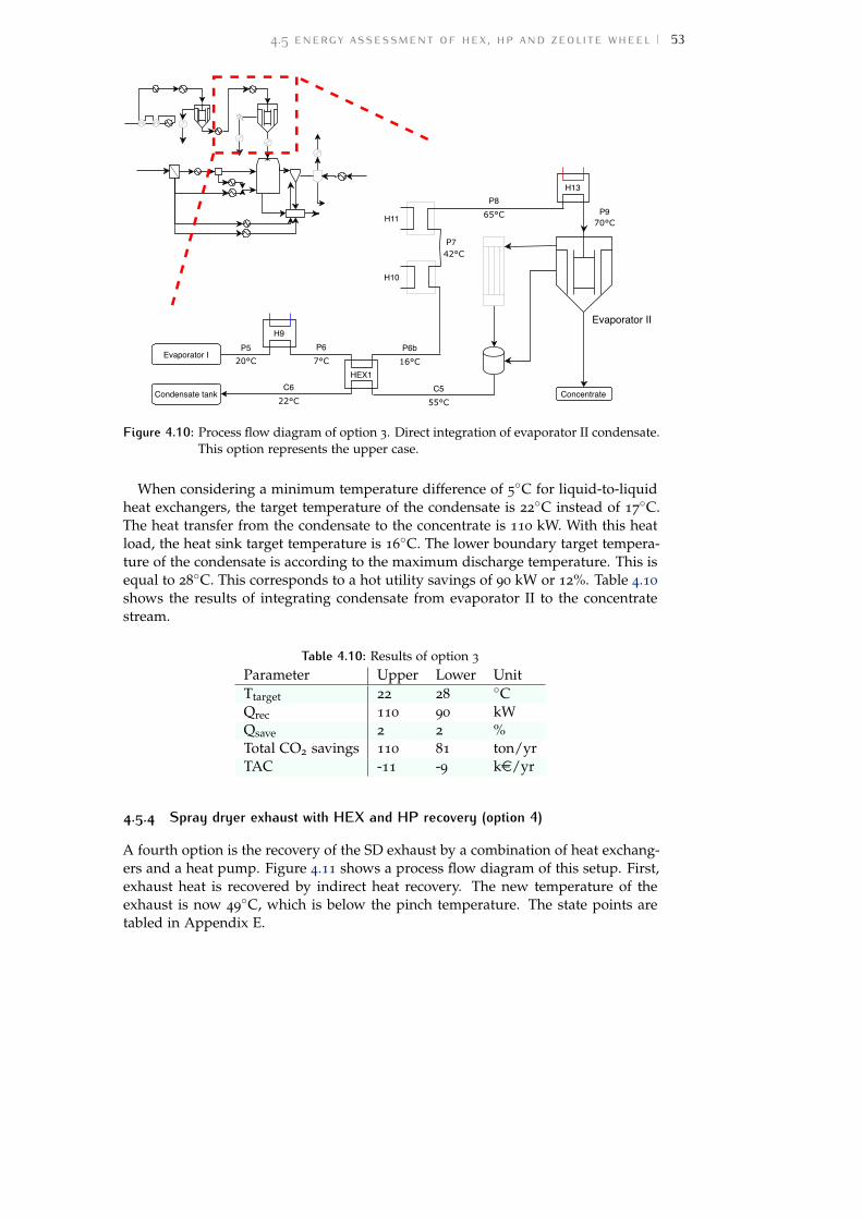
4.5 energy assessment of hex, hp and zeolite wheel 53
Concentrate
P6 P6b
H13
H9Evaporator II
C5HEX1
C6Condensate tank
Evaporator I
P865°C P9
70°C
16°C
55°C22°C
7°CP520°C
P742°C
H11
H10
Figure 4.10: Process flow diagram of option 3. Direct integration of evaporator II condensate.This option represents the upper case.
When considering a minimum temperature difference of 5C for liquid-to-liquid
heat exchangers, the target temperature of the condensate is 22C instead of 17
C.The heat transfer from the condensate to the concentrate is 110 kW. With this heatload, the heat sink target temperature is 16
C. The lower boundary target tempera-ture of the condensate is according to the maximum discharge temperature. This isequal to 28
C. This corresponds to a hot utility savings of 90 kW or 12%. Table 4.10
shows the results of integrating condensate from evaporator II to the concentratestream.
Table 4.10: Results of option 3
Parameter Upper Lower UnitTtarget 22 28
CQrec 110 90 kWQsave 2 2 %Total CO2 savings 110 81 ton/yrTAC -11 -9 ke/yr
4.5.4 Spray dryer exhaust with HEX and HP recovery (option 4)
A fourth option is the recovery of the SD exhaust by a combination of heat exchang-ers and a heat pump. Figure 4.11 shows a process flow diagram of this setup. First,exhaust heat is recovered by indirect heat recovery. The new temperature of theexhaust is now 49
C, which is below the pinch temperature. The state points aretabled in Appendix E.

54 results
Spray Dryer
Heater
HEX 2
Ambient air
HEX1
AX1 AX2 AX3 AX4
AX5
67°C 37°C
77°C49°C
20°C 57°C 190°C
Ambient air
AX6
AX7
72°C
40°C
Figure 4.11: Process flow diagram of option 4. Integration of heat pump combined withliquid loop indirect heat recovery of spray dryer. This option represents theupper case.
After indirect heat recovery, the stream enters the evaporator of the heat pump.This stream serves as the heat source. Target temperatures of 40 and 45
C are cho-sen as respectively upper and lower cases.
In the upper case, which is represented in figure 4.11, the heat sink target tem-perature is 72
C, with a COP of 5.1. In comparison, the target temperature in thelower case is 63
C, with a COP of 7.8. The curves in figure 4.12 represent differentheat source target temperatures, when the heat source supply temperature is con-stant. Most energy is saved when the target temperature is at the upper boundaryof 40
C. This is indicated by the solid line in figure 4.12.
0
2
4
6
8
10
12
14
16
60 65 70 75 80 85
CO
P
Tt,sink (°C)
Upper @40°C
Lower @45°C
Figure 4.12: Heat sink target temperature for upper and lower heat source target tempera-tures. The supply temperatures remain constant at 49 and 57
C.
The specifications of the heat pump design are shown in table 4.11. For givenupper and lower scenarios, the associated heat duty and temperatures are listed.There exists an energy balance in the evaporator and the condenser. This meansthat the heat, which is absorbed and accumulated by the refrigerant, is the same asheat from the heat sink and to the heat source.
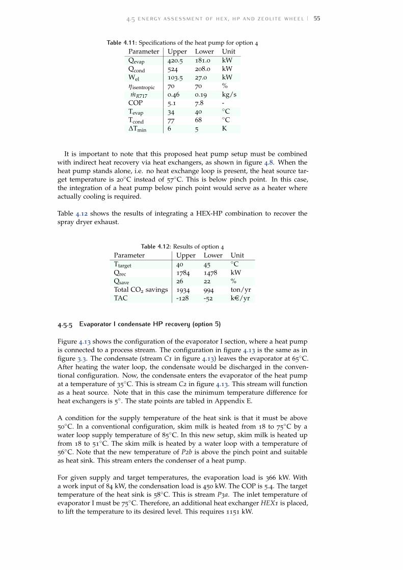
4.5 energy assessment of hex, hp and zeolite wheel 55
Table 4.11: Specifications of the heat pump for option 4
Parameter Upper Lower UnitQevap 420.5 181.0 kWQcond 524 208.0 kWWel 103.5 27.0 kWηisentropic 70 70 %mR717 0.46 0.19 kg/s
COP 5.1 7.8 -Tevap 34 40
CTcond 77 68
C∆Tmin 6 5 K
It is important to note that this proposed heat pump setup must be combinedwith indirect heat recovery via heat exchangers, as shown in figure 4.8. When theheat pump stands alone, i.e. no heat exchange loop is present, the heat source tar-get temperature is 20
C instead of 57C. This is below pinch point. In this case,
the integration of a heat pump below pinch point would serve as a heater whereactually cooling is required.
Table 4.12 shows the results of integrating a HEX-HP combination to recover thespray dryer exhaust.
Table 4.12: Results of option 4
Parameter Upper Lower UnitTtarget 40 45
CQrec 1784 1478 kWQsave 26 22 %Total CO2 savings 1934 994 ton/yrTAC -128 -52 ke/yr
4.5.5 Evaporator I condensate HP recovery (option 5)
Figure 4.13 shows the configuration of the evaporator I section, where a heat pumpis connected to a process stream. The configuration in figure 4.13 is the same as infigure 3.3. The condensate (stream C1 in figure 4.13) leaves the evaporator at 65
C.After heating the water loop, the condensate would be discharged in the conven-tional configuration. Now, the condensate enters the evaporator of the heat pumpat a temperature of 35
C. This is stream C2 in figure 4.13. This stream will functionas a heat source. Note that in this case the minimum temperature difference forheat exchangers is 5
. The state points are tabled in Appendix E.
A condition for the supply temperature of the heat sink is that it must be above50C. In a conventional configuration, skim milk is heated from 18 to 75
C by awater loop supply temperature of 85
C. In this new setup, skim milk is heated upfrom 18 to 51
C. The skim milk is heated by a water loop with a temperature of56C. Note that the new temperature of P2b is above the pinch point and suitable
as heat sink. This stream enters the condenser of a heat pump.
For given supply and target temperatures, the evaporation load is 366 kW. Witha work input of 84 kW, the condensation load is 450 kW. The COP is 5.4. The targettemperature of the heat sink is 58
C. This is stream P3a. The inlet temperature ofevaporator I must be 75
C. Therefore, an additional heat exchanger HEX1 is placed,to lift the temperature to its desired level. This requires 1151 kW.

56 results
Skim milk
P1
P2a
P4
P5
W1W2
W3W4
C1
C2
H7
H5
H6 H8
Evaporator I
Condensatetank
P2b
C3
Evaporator II
65°C
20°C10°C
18°C
65°C
35°C
48°C56°C
23°C23°C
28°C
51°C
P3a58°C
HEX1
P3b75°C
Figure 4.13: Process flow diagram of option 5. Heat pump integration in evaporation I sec-tion. This diagram represents the upper case
Figure 4.14 shows the COP curves for the upper and lower case. At an optimalcase, the supply temperature is 35
C and the target temperature is 28C. The COP
is 5.4. The lower case is at a supply temperature of 39C and a target temperature
of 35C. The COP is 9.8.
0
2
4
6
8
10
12
14
16
52 54 56 58 60 62 64
CO
P
Tt,sink (°C)
Upper @35°C
Lower @39°C
Figure 4.14: COP curves for supply temperature of 35 and 39C. Heat source target temper-
atures were 28C (35
C) and 35C (39
C).
The specifications for the heat pump design are shown in figure 4.13.
Table 4.13: Specifications of the heat pump for option 5
Parameter Upper Lower UnitQevap 366 210 kWQcond 450 244 kWWel 84 34 kWηisentropic 70 70 %mR717 0.37 0.21 kg/s
COP 5.4 7.2 -Tevap 23 30
CTcond 63 60
C∆Tmin 5 5 K
The upper and lower case are based on heat surplus of stream C3 and heat de-mand of heat exchangers H7 and HEX1. Regarding the heat surplus, the targettemperatures in these cases are 28 and 35
C. This is far above the minimum dis-charge temperature of 11
C. When the streams in the upper and lower case arerecovered until this temperature, respectively 888 and 1254 kW is available. Regard-

4.5 energy assessment of hex, hp and zeolite wheel 57
ing heat exchanger H7, this is a steam heat exchanger which partly heats a waterloop. Both the upper and lower case are based on heat demand of heat exchangerH7. When more heat from the condensate, immediately leaving the evaporator, canbe recovered by heat exchanger H8, less hot utility is required. Compared to theconventional water loop, which requires 2133 kW (see Appendix B at H7), the newwater loop requires 517 and 726 kW in respectively the upper and lower case. Ad-ditionally, heat exchanger HEX1 requires in this new setup 1074 and 1283 kW forrespectively the upper and lower case. Taking into account both the new demandof H7 and HEX1 and the possibility of recovering heat from stream C3
, 1430 (uppercase) and 1378 (lower case) kW can be recovered. It must be emphasized that option5 is only beneficial to energy savings when heat from C3 is recovered.
Table 4.14 summarizes the results of heat pump recovery of condensate from evap-orator I.
Table 4.14: Results of option 5
Parameter Upper Lower UnitTsupply 35 39
CQrec 1430 1378 kWQsave 21 20 %Total CO2 savings 1569 902 ton/yrTAC -145 -86 ke/yr
4.5.6 Evaporator II condensate HP recovery (option 6)
A sixth option is the heat pump integration at the condensate stream of evaporatorII. In the evaporator II section, condensate leaves the process and is dischargedwithout any heat recovery. Referring to figure 3.3, in reality the condensate streamdirectly flows to a tank after being discharged at a temperature of 55
C. Figure 4.15
shows a setup of the integration of the heat pump. The state points are tabled inAppendix E.
P10
Concentrate
Condensatetank
P5 P6
P7
P9
P8
V3
W5
W6
W7
C3
H9
H10
H11
H12
C4
Evaporator II
C5
7°C
42°C
66°C
70°C
55°C
55°C
55°C
55°C
49°C
45°C
81°C
77°C
20°C
C637°C
Evaporator I
Figure 4.15: Process flow diagram of option 6. Flow diagram of heat pump integration inevaporator II section. This figure represents the upper case.
In this new setup, the condensate streams C3 and C4 are collected in a tank. Thisoccurs at a temperature of 55
C. The stream leaving the tank will be the heat sourcein the heat pump. A prerequisite is that this stream is below 50
C. For this analysisit is assumed that the stream will leave the tank at 49
C. An option for cooling is toindirectly cool the tank with tap water or ambient air.

58 results
The concentrate entering evaporator II functions as a heat sink. This stream isfirst cooled down to 7
C, indicated by heat exchanger H9 in figure 4.15. In the basecase, the concentrate is heated to 70
C by a water loop and a steam heat exchanger.In this new setup, the heat pump replaces the steam injected heat exchanger. Nowthe concentrate is heated by both the water loop and the heat pump as shown inthe figure. A prerequisite is that the heat sink target temperature is 70
C, shown bystream P9 in figure 4.15.
This option has only one setup, i.e. no lower and upper boundary. The reasonfor this is the prerequisite of a COP of 5 and the evaporation and condensationtemperatures in the heat pump. The only setup which meets the statements of theHP decision tree is shown in figure 4.15. The COP graph is shown in figure 4.16.
0
2
4
6
8
10
12
14
16
69,0 69,5 70,0 70,5 71,0 71,5 72,0 72,5 73,0
COP
Tt,sink (°C)
Figure 4.16: COP curve for supply temperature of 66C. Option 6 has one case
The specifications of the heat pump design are shown in table 4.15:
Table 4.15: Specifications of the heat pump for option 6
Parameter Optimal UnitQevap 38 kWQcond 47 kWWel 9 kWηisentropic 70 %mR717 0.04 kg/s
COP 5.05 -Tevap 32
CTcond 75
C∆Tmin 5.6 K
Table 4.16 shows the results of option 6. Note that the setup is divided in a upperand lower case.
Table 4.16: Results of option 6
Parameter Upper Lower UnitTsupply 66 66
CQrec 133 133 kWQsave 2 2 %Total CO2 savings 146 92 ton/yrTAC -5 -5 ke/yr

4.5 energy assessment of hex, hp and zeolite wheel 59
4.5.7 Spray dryer exhaust zeolite wheel recovery (option 7)
Figure 4.17 shows a schematic flow diagram with temperatures of a zeolite wheelcoupled to a spray dryer and a super-heated steam (SHS) loop.
Dryer Adsorber Regenerator Steam surplus
Concentrate
Milk powder
A20
A21
HEX2
Ambient air
A22
A23
Ambient air
SHS-loop
S1
S2
S3S4
A24
A25HEX1
A26150°C190°C
55°C
77°C20°C
77°C
77°C
3014 kJ/kg
1120 kJ/kg
1120 kJ/kg
1120 kJ/kg
Figure 4.17: Process flow diagram of option 7. A spray dryer with integrated zeolite system.
The left part of figure 4.17 represents the spray dryer. First, the exhaust air leavesthe spray dryer, denoted by A20 in figure 4.17. This stream has an AH of 0.04
kg/kgda, a temperature of 77C and a mass flow rate of 45 kg/s. The mass flow
rate must be reduced to be equal to the spray dryer inlet mass flow rate. To pro-duce skim milk powder, the spray dryer requires an inlet mass flow rate of 34
kgda/s. Stream A21 represents the discharge of surplus air, resulting in streamA22. Subsequently, this stream is mixed with ambient air, so the flow rate of streamA24 is 34 kgda/s This stream is mixed with ambient air, to reduce the AH to 0.026
kg/kgda. The AH level must be reduced because of the maximum water loadingof zeolite. This will be described further on in this section. However, mixing thestream with ambient air also reduces the temperature of air to 55
C. After mixing,the air enters the adsorption unit of the zeolite wheel and leaves as dehumidifiedprocessed air. The state points of the zeolite configuration are found in Appendix G.
The zeolite adsorbs 0.024 kg/kg moisture from the exhaust air. The MRC of theadsorption unit is then 0.82 kg/s. By knowing the MRC, the total amount of heatreleased from the zeolite to the air is calculated. Table 4.17 shows the energy bal-ance of the adsorption unit. In Appendix F, the input variables for the zeolite wheelare shown. The total heat transferred to the air is negative because heat is extractedfrom the adsorption unit.
Table 4.17: Energy balance of adsorption unitParameter Value UnitMRC 0.82 kg/sHeat of adsorption -979 kWHeat inlet 4155 kWHeat outlet 5134 kW
The adsorption outlet temperature of air is 150C. This stream (A25 in figure 4.17)
is heated up by HEX1 to the desirable inlet temperature, i.e. 190C. The heat duty
of the heat exchanger is 1348 kW to heat the airflow from 150 to 190C. Figure 4.18
shows a Mollier chart of the airside of the zeolite wheel with state points, whichcorrespond to figure 4.17. This setup is an open cycle, where both surplus air isdischarged and exhaust is mixed with ambient air. Although not shown in thefigure, ambient air is mixed with the exhaust (A20). This results in a movement toadsorption inlet flow (A24). The zeolite decreases humidity in the exhaust air andthe temperature of the air increases due to latent and adsorption heat (A25). A final

60 results
heat exchanger (HEX1) increased the temperature to a desirable level (A26). In thespray dryer, temperature of the air decreases and AH increases (A20).
A26
A20
A24
A25
HEX1
ZW
SD
Tamb
Mixer
0
0,02
0,04
0,06
0,08
0,1
0,12
0 20 40 60 80 100 120 140 160 180 200
AH
(kg
w/k
g da)
Temperature (°C)
Figure 4.18: Mollier chart of the airside of an open loop zeolite wheel configuration.
Referring to table 4.17, the MRC is 0.82 kg/s. This means that the steam surplusis also 0.82 kg/s. The regeneration temperature of the regeneration steam inlet is270C with a mass flow of 1 kg/s. The mass flow is chosen as an illustrative reason.
Steam enters the regenerator with a heat load of 2790 kW. The steam provides thedesorption heat for the release of moisture from the zeolite. The desorption heatis equal to the adsorption heat. In this case 0.024 kgw/kg is desorbed to steam.Additionally, heat of vaporization is released to the regeneration medium.
With an inlet mass flow rate of 1 kg/s, the steam leaves the regenerator with 1.82
kg/s. This stream has a heat load of 1810 kW. This enthalpy is the difference ofthe steam inlet and the desorption heat. After regeneration, steam surplus leavesthe sorption system. This is stream S2 in figure 4.17. Valorization of this streamresults in additional useful heat with a heat load of 914 kW. Stream S3 in figure4.17, now has a mass flow rate of 1 kg/s and is ready to be heated to 270
C. Theheat exchanger HEX2 needs 1793 kW to raise the steam temperature to 270
C.
Although the regeneration of zeolite requires high temperatures, a zeolite wheelmay decrease spray drying energy consumption. In the regeneration section, steamneeds to be heated by a heat exchanger. With a mass flow rate of 1 kg/s, heatexchanger HEX2 in figure 4.17 requires 1893 kW. However, when steam surplus isused in another part of the process, the net energy demand of the regenerator maybe 1893-914=979 kW. To research the effect of SHS mass flow rate, different valueswere used. However, net energy demand will not change for different steam massflow rates.
In total, the spray dryer with zeolite wheel has a net energy demand of 1372+979=2351
kW. Table 4.18 shows the results. A conventional spray dryer needs 5831 kW to heatambient air to 190
C. Therefore, a zeolite wheel can have a net hot utility saving of3480 kW.
Table 4.18: Zeolite heat requirement overview.Process Q[-] [kW]HEX1 1372
HEX2 1893
Steam surplus -914
SD net energy demand 2351

4.5 energy assessment of hex, hp and zeolite wheel 61
Table 4.19 shows the results of the zeolite wheel.
Table 4.19: Results of option 7
Parameter Upper Lower UnitQrec 3480 3480 kWQsave 51 51 %Total CO2 savings 3806 3110 ton/yrTAC -123 -15 ke/yr

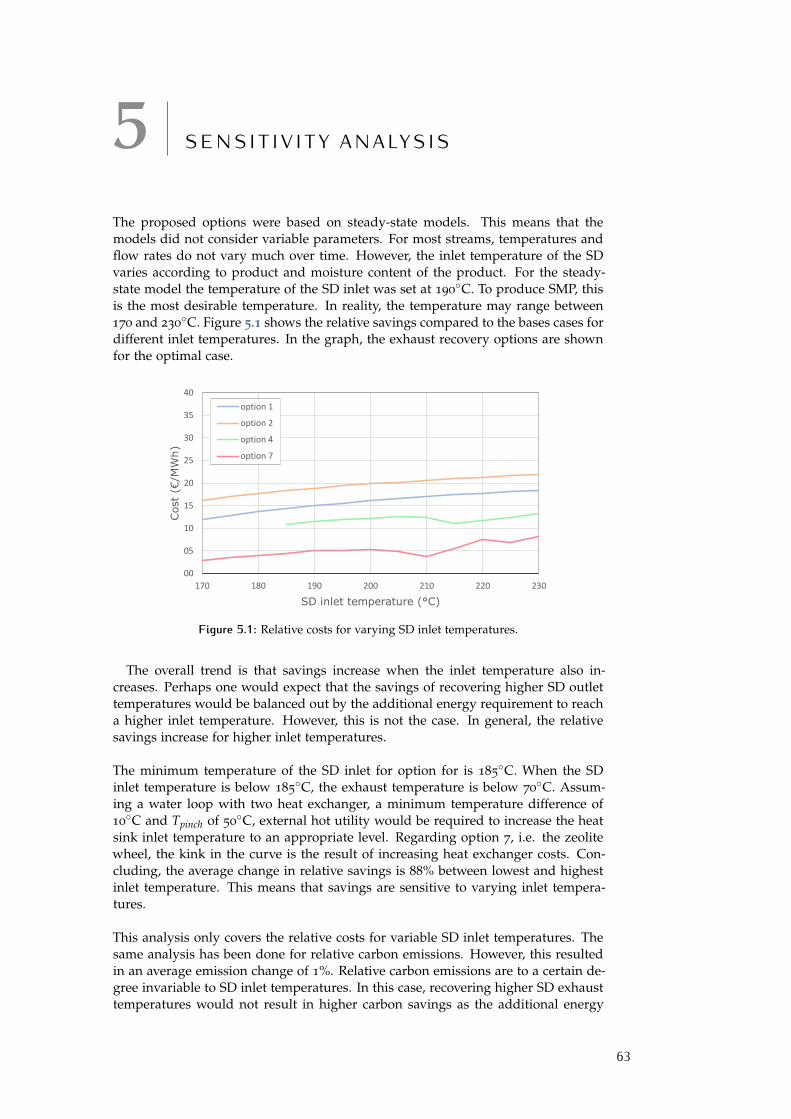
5 S E N S I T I V I T Y A N A LY S I S
The proposed options were based on steady-state models. This means that themodels did not consider variable parameters. For most streams, temperatures andflow rates do not vary much over time. However, the inlet temperature of the SDvaries according to product and moisture content of the product. For the steady-state model the temperature of the SD inlet was set at 190
C. To produce SMP, thisis the most desirable temperature. In reality, the temperature may range between170 and 230
C. Figure 5.1 shows the relative savings compared to the bases cases fordifferent inlet temperatures. In the graph, the exhaust recovery options are shownfor the optimal case.
00
05
10
15
20
25
30
35
40
170 180 190 200 210 220 230
Cost
(€/M
Wh)
SD inlet temperature (°C)
option 1
option 2
option 4
option 7
Figure 5.1: Relative costs for varying SD inlet temperatures.
The overall trend is that savings increase when the inlet temperature also in-creases. Perhaps one would expect that the savings of recovering higher SD outlettemperatures would be balanced out by the additional energy requirement to reacha higher inlet temperature. However, this is not the case. In general, the relativesavings increase for higher inlet temperatures.
The minimum temperature of the SD inlet for option for is 185C. When the SD
inlet temperature is below 185C, the exhaust temperature is below 70
C. Assum-ing a water loop with two heat exchanger, a minimum temperature difference of10C and Tpinch of 50
C, external hot utility would be required to increase the heatsink inlet temperature to an appropriate level. Regarding option 7, i.e. the zeolitewheel, the kink in the curve is the result of increasing heat exchanger costs. Con-cluding, the average change in relative savings is 88% between lowest and highestinlet temperature. This means that savings are sensitive to varying inlet tempera-tures.
This analysis only covers the relative costs for variable SD inlet temperatures. Thesame analysis has been done for relative carbon emissions. However, this resultedin an average emission change of 1%. Relative carbon emissions are to a certain de-gree invariable to SD inlet temperatures. In this case, recovering higher SD exhausttemperatures would not result in higher carbon savings as the additional energy
63

64 sensitivity analysis
requirement in the boilers balances out the emission savings.
Another parameter which is variable is the heat sink target temperature of heatpump configurations. In the case of HP integration in the evaporator I and II sec-tion, the heat sink target temperature is fixed. This is because the inlet temperatureof the evaporators is fixed. Because of fixed target temperatures, there is little roomto vary the COP. On the contrary, the heat sink target temperature is not fixed forthe HP, recovering SD exhaust. Figure 5.2 shows the effect of changing the COP onthe total cost and carbon savings for option 4.
1130
1230
1330
1430
1530
1630
1730
0
50
100
150
200
250
300
0 5 10 15 20
CO
2-e
(to
n)
Savi
ngs
(k€)
COP
Figure 5.2: The effect of varying COP values on annual savings and CO2-e savings for option4.
Low COP values result in high work input. This in turn, results in high thermalenergy savings. However, shown in figure 5.2, both cost and carbon savings arerelatively low when the COP is low. When the COP increases, savings are higher.The same applies to carbon savings. Interesting to note, most carbon is saved whenthe COP is highest. Simultaneously, when the COP is highest, the heat sink targettemperature is lowest. One would assume that lower target temperatures result inlower carbon savings, as more external hot utility is required. However, a higherCOP means more electricity input. The large amount of electricity, combined withits carbon intensity, cancels out the advantage of a high heat sink target temperaturein terms of carbon savings. The graph shows that both cost and carbon savings aresensitive to change in COP.

6 D I S C U S S I O N
6.1 discussion of the model and input data
The basis for all the results is the data process sheet in figure 4.2. To some extent,both drawing the process flow and retrieving process data is done at a degree ofuncertainty. For instance, it is assumed that only SMP is produced. In reality, twelvedifferent products are produced. Every product has its unique setpoints at whichthe process operates. Furthermore, the case study is part of a larger factory withmultiple production lines. In addition to the case study, two similar productionlines and a cheese factory are present at the site. Clearly, including every setpointand production line, would add major complexity to the model. Besides complex-ity, another reason for focusing on one process was present. The evaporators andthe spray dryer in the case study are recently installed. Assuming a lifetime of 20
years, these installations will still be operational for a long period of time. On thecontrary, the two other production lines, which are not included in the model, willbe replaced in the near future. Researching heat recovery for these production linesis a waste of time as they will be replaced soon. It becomes a more compelling rec-ommendation to convince decision-makers when the lifetime of operational units islonger. When the two production lines will be replaced, the findings of this studycan function as a blueprint for assessing heat recovery options. Future study aboutthe applicability of heat recovery technologies for different milk powder productsmay then be interesting.
The model in this study is based on a continuous process. This means that startup,shutdown, batch and CIP procedures are not considered. Incorporating these pro-cedures in this model, could mean including a time-dependent pinch analysis. Re-garding CIP, this is a significant part of heating demand in the milk powder process[24]. The consideration of whether or not to include CIP in the model is based onthe occurrence of the CIP stream. A concern is the availability of this stream. Forexample, cleaning a spray dryer occurs every four weeks. Although the energy de-mand is high when this happens, including such an incidental stream in a pinchanalysis is unnecessary. On the contrary, cleaning evaporators is done daily. How-ever, the availability of proper heat sources or sink to connect with a CIP streamis a problem. Clearly, during CIP, the production process is down. Therefore, non-operational procedures are excluded. Despite the simplification of the model, thefindings in this study do say something about recovering heat when the process isoperating.
An implication for excluding above-mentioned processes is monotone data. Massflow rates and temperatures are based on continuous flows. In reality flow rates andtemperatures differ according to product and process. Another aspects which sim-plifies the model but also affects stream properties, is the exclusion of (buffer)tanks.In reality there are (buffer)tanks between every section. The flow and temperaturechange before and after a tank. Because tanks are excluded, this results in disparityof flow rates and temperatures. In such cases, the leading stream specifications arethe ones from the inlet stream. Furthermore, heat loss is neglected. Reason for thisis to reduce workload and complexity. Adding unit-specific heat loss data wouldrequire detailed information.
65

66 discussion
The environmental analysis is based on data which are subject to a degree of uncer-tainty. The indirect carbon emissions of the three technologies is based on both LCAstudies, the performance of technologies and a scaling factor. Heat pump LCA stud-ies are overrepresented in academic literature. The abundance of studies resulted inthe problem for which LCA study to select for calculating indirect carbon emissionsfor the heat pump. By specifying boundary and functional unit, one study was se-lected. On the contrary, only one LCA about heat exchangers was found. As thereare no other LCA studies to compare with, the findings of indirect carbon emis-sions from heat exchangers is less substantiated. Regarding the zeolite wheel, noLCA studies or other environmental assessments studies are available. In absenceof these studies, the nearest approach for defining indirect carbon emissions, is tobreak down the wheel into multiple material components. Although this is not afounded method to calculate indirect carbon emissions, it gives an indication of theamount of carbon emitted during its manufacturing process. Other doubtful param-eters in estimating indirect carbon emissions, are the scaling factor and dimensionfactor. The idea behind the scaling factor is to balance the LCA boundary of thereference with the case study. The problem with this is that it assigns the samecarbon intensity to different processes. For instance, the indirect carbon emissionsfor the zeolite wheel are based on the carbon intensity of mining and processing theraw materials from which the wheel is composed. This carbon intensity number isthen multiplied by a factor to also include assembling, transportation etc. However,assembling, transportation etc. may have different carbon intensities. To put thescaling factor in perspective though, increasing the factor 1000% still only results ina share of 5% of direct carbon emissions relative to total emissions. Another param-eter which raises uncertainty is the dimension factor. This factor is added to balancethe carbon intensity of the reference technology with the case study technology bycomparing their performances. A problem with this approach is the assumptionthat the relationship between performance, i.e. HEX area, condensation heat orMRC, and indirect carbon emissions is linear. A recommendation for future studyis to conduct an LCA for the zeolite wheel, to research the relation between car-bon emissions and functional unit. In addition to indirect carbon emission, directcarbon emissions are calculated. Due to a more straightforward approach, directcarbon emissions have higher degree of certainty.
Regarding the economic analysis the same challenge arises. The capital costs of thetechnologies are based on both the Lang Factor and the dimensions of references.For the Lang Factor a reasonable value was chosen [34]. However, the dimensionfactor for investment costs has the same implication as in the environmental analy-sis; a linear relation between technology performance and capital costs. Especiallyfor estimating costs of the zeolite wheel, information is less available. Although theinvestment costs are subject to uncertainty, the utility and carbon costs are estimatedwith more confidence.
6.2 discussion of resultsThis study assesses heat recovery technologies on thermal, environmental and eco-nomic performance. Figure 6.1 shows the results of the different technologies onenergy use (6.1a), environment (6.1b) and economy (6.1c). The figures show bothupper and lower cases. In terms of thermal energy savings, four configurationsperform above average. First, the zeolite wheel has the most gain in energy savings,i.e. 3480 kW. This is caused by the recovery of latent heat from the exhaust. Otheroptions which have a significant effect on energy savings are option 2, 4 and 5. Re-garding option 2, directly recovering the SD exhaust, results in more saved energy.From an energy standpoint, direct energy recovery is more desirable than indirect
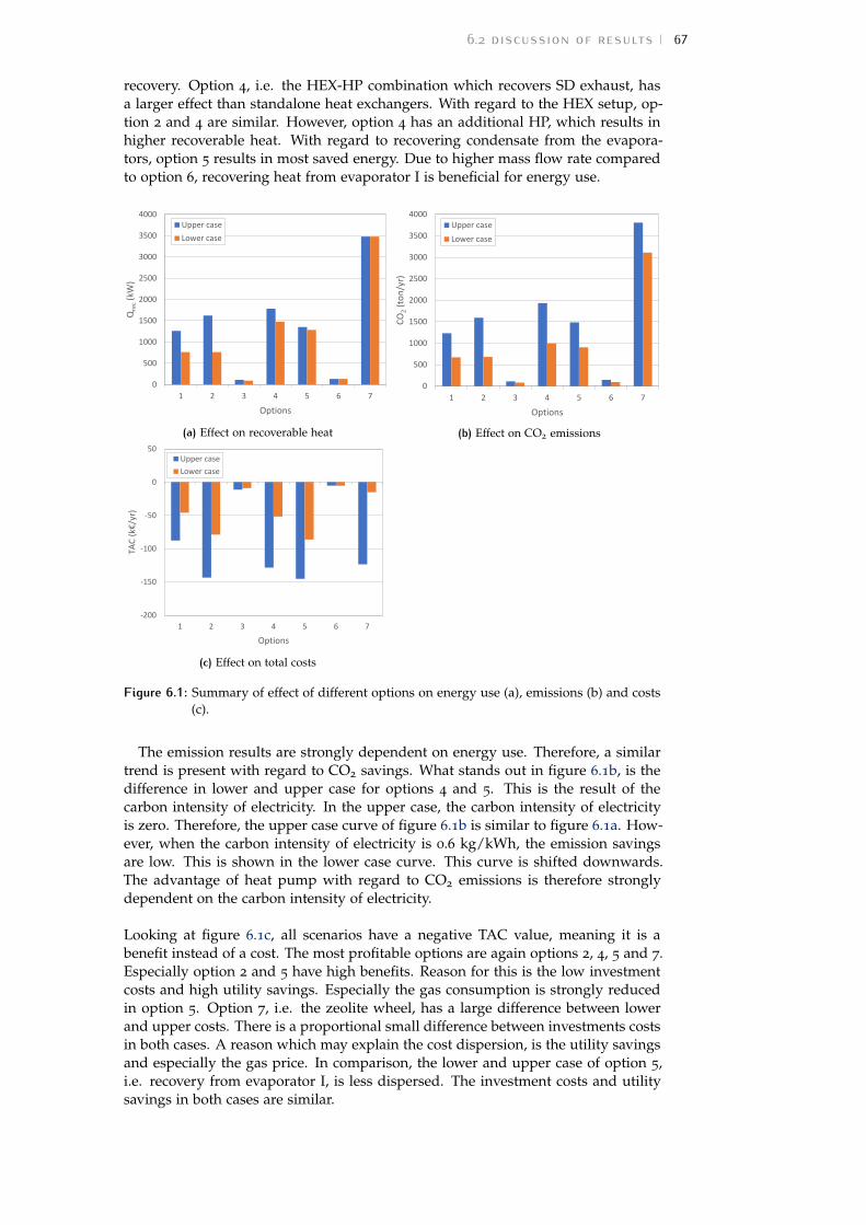
6.2 discussion of results 67
recovery. Option 4, i.e. the HEX-HP combination which recovers SD exhaust, hasa larger effect than standalone heat exchangers. With regard to the HEX setup, op-tion 2 and 4 are similar. However, option 4 has an additional HP, which results inhigher recoverable heat. With regard to recovering condensate from the evapora-tors, option 5 results in most saved energy. Due to higher mass flow rate comparedto option 6, recovering heat from evaporator I is beneficial for energy use.
0
500
1000
1500
2000
2500
3000
3500
4000
1 2 3 4 5 6 7
Qre
c(k
W)
Options
Upper case
Lower case
(a) Effect on recoverable heat
0
500
1000
1500
2000
2500
3000
3500
4000
1 2 3 4 5 6 7C
O2
(to
n/y
r)
Options
Upper case
Lower case
(b) Effect on CO2 emissions
-200
-150
-100
-50
0
50
1 2 3 4 5 6 7
TAC
(k€
/yr)
Options
Upper case
Lower case
(c) Effect on total costs
Figure 6.1: Summary of effect of different options on energy use (a), emissions (b) and costs(c).
The emission results are strongly dependent on energy use. Therefore, a similartrend is present with regard to CO2 savings. What stands out in figure 6.1b, is thedifference in lower and upper case for options 4 and 5. This is the result of thecarbon intensity of electricity. In the upper case, the carbon intensity of electricityis zero. Therefore, the upper case curve of figure 6.1b is similar to figure 6.1a. How-ever, when the carbon intensity of electricity is 0.6 kg/kWh, the emission savingsare low. This is shown in the lower case curve. This curve is shifted downwards.The advantage of heat pump with regard to CO2 emissions is therefore stronglydependent on the carbon intensity of electricity.
Looking at figure 6.1c, all scenarios have a negative TAC value, meaning it is abenefit instead of a cost. The most profitable options are again options 2, 4, 5 and 7.Especially option 2 and 5 have high benefits. Reason for this is the low investmentcosts and high utility savings. Especially the gas consumption is strongly reducedin option 5. Option 7, i.e. the zeolite wheel, has a large difference between lowerand upper costs. There is a proportional small difference between investments costsin both cases. A reason which may explain the cost dispersion, is the utility savingsand especially the gas price. In comparison, the lower and upper case of option 5,i.e. recovery from evaporator I, is less dispersed. The investment costs and utilitysavings in both cases are similar.
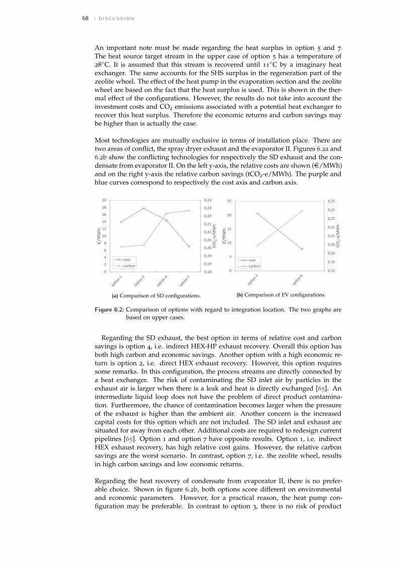
68 discussion
An important note must be made regarding the heat surplus in option 5 and 7.The heat source target stream in the upper case of option 5 has a temperature of28C. It is assumed that this stream is recovered until 11
C by a imaginary heatexchanger. The same accounts for the SHS surplus in the regeneration part of thezeolite wheel. The effect of the heat pump in the evaporation section and the zeolitewheel are based on the fact that the heat surplus is used. This is shown in the ther-mal effect of the configurations. However, the results do not take into account theinvestment costs and CO2 emissions associated with a potential heat exchanger torecover this heat surplus. Therefore the economic returns and carbon savings maybe higher than is actually the case.
Most technologies are mutually exclusive in terms of installation place. There aretwo areas of conflict, the spray dryer exhaust and the evaporator II. Figures 6.2a and6.2b show the conflicting technologies for respectively the SD exhaust and the con-densate from evaporator II. On the left y-axis, the relative costs are shown (e/MWh)and on the right y-axis the relative carbon savings (tCO2-e/MWh). The purple andblue curves correspond to respectively the cost axis and carbon axis.
0,18
0,19
0,19
0,20
0,20
0,21
0,21
0,22
0,22
0,23
0
2
4
6
8
10
12
14
16
18
20
tCO2-e/MWh
€/MWh
cost
carbon
(a) Comparison of SD configurations.
0,19
0,19
0,20
0,20
0,21
0,21
0,22
0,22
0,23
0
5
10
15
20
25
tCO2-e/M
Wh
€/MWh
cost
carbon
(b) Comparison of EV configurations.
Figure 6.2: Comparison of options with regard to integration location. The two graphs arebased on upper cases.
Regarding the SD exhaust, the best option in terms of relative cost and carbonsavings is option 4, i.e. indirect HEX-HP exhaust recovery. Overall this option hasboth high carbon and economic savings. Another option with a high economic re-turn is option 2, i.e. direct HEX exhaust recovery. However, this option requiressome remarks. In this configuration, the process streams are directly connected bya heat exchanger. The risk of contaminating the SD inlet air by particles in theexhaust air is larger when there is a leak and heat is directly exchanged [65]. Anintermediate liquid loop does not have the problem of direct product contamina-tion. Furthermore, the chance of contamination becomes larger when the pressureof the exhaust is higher than the ambient air. Another concern is the increasedcapital costs for this option which are not included. The SD inlet and exhaust aresituated for away from each other. Additional costs are required to redesign currentpipelines [65]. Option 1 and option 7 have opposite results. Option 1, i.e. indirectHEX exhaust recovery, has high relative cost gains. However, the relative carbonsavings are the worst scenario. In contrast, option 7, i.e. the zeolite wheel, resultsin high carbon savings and low economic returns.
Regarding the heat recovery of condensate from evaporator II, there is no prefer-able choice. Shown in figure 6.2b, both options score different on environmentaland economic parameters. However, for a practical reason, the heat pump con-figuration may be preferable. In contrast to option 3, there is no risk of product

6.3 discussion of results in comparison with existing literature 69
contamination with a heat pump because the product streams are not directly con-nected to each other.
6.3 discussion of results in comparison with ex-isting literature
In terms of absolute energy savings, the zeolite wheel is preferred with a savingsof 2.3 MJ/kgsmp. This is a reduction of 60% of thermal energy in the SD. This wasin line with expectations, as other studies found a thermal energy reduction of 60%[34], 59% [31] and 50% [35]. Another option with a high impact on hot utility use,is the HEX-HP combination recovering heat from the SD exhaust. This resulted ina savings of 1.2 MJ/kgsmp, or 30% thermal energy reduction in the SD. For similarinput temperatures, exhaust temperatures and minimum temperature differences,other studies found a hot utility reduction of 40% [26] or 47% [27]. A first reasonwhich may explain the discrepancy in results between this study and existing stud-ies, is the COP value of the HP. There is a trade-off between COP and heat recovery.When the COP is low, thus proportionally more work input, the heat recovery ishigh. And vice versa. The studies in [26] and [27] used COP values between 1.5and 4.5. The minimum COP value in this study was set at 5. Another explanationfor the difference in heat recovery percentage is the evaporator outlet temperatures.The two studies show heat recovery options until an evaporator outlet temperatureof 20
C [26, 27]. On the contrary, this study shows recovery until its dew point.Future research can focus on the effect of working fluid in HP configuration for SDexhaust recovery.
Academic studies about carbon savings of SD heat recovery technologies is lessabundant. However, [28] found a carbon reduction of 43% for HP-HEX exhaustrecovery. In this study, HP-HEX exhaust recovery results in a carbon reductionof 27% compared to the base case. Regarding [28], the energy savings are largercompared to this study, resulting in higher direct carbon savings. Another factorwhich may explain the difference in carbon savings is the chosen value of specificcarbon emission of natural gas and electricity. This study focused on assessing thecarbon emissions for the whole life cycle of different technologies, without conduct-ing an LCA. In particular for heat exchangers and zeolite wheels, rigorous carbonassessments are required. To fully understand the carbon emissions of these twotechnologies, future studies may look at doing an LCA.
No similar economic assessments were available for comparison. In contrast, an-other cost assessment was done by [34] for the zeolite wheel. The EAC of thezeolite wheel are similar. Regarding the heat pump configuration, option 5, i.e. HPcondensate I recovery, is most profitable in terms of costs. This option can save 108
ke/year. Other heat pump cost assessments found a maximum potential savingsof 440 ke/year [29] and 942 ke/year [24]. The difference can be explained by typeof heat pump. For instance, [24] selected a MVR to decrease energy consumptionof the evaporator. This heat pump setting saves more energy, and thus utility andcarbon costs.


7 C O N C L U S I O N
With a growing world population, pressure on food production is an inevitableconsequence. The responsible sector for feeding the world is the agricultural sec-tor. A big contributor within agriculture is the dairy industry. Zooming in on theEU, the dairy industry accounts for 28% of total food consumption [6]. Most ofthese dairy products is also produced in the EU, as it is one of the largest globalproducers of dairy products. Approximately 20% of global dairy output originatesfrom the EU [2]. The character and magnitude of the agricultural sector, and specifi-cally the dairy industry, result in a large demand of energy. Big part of this energy isprovided by fossil fuels and eventually used for the industrial production of agricul-tural products. A combination of increased production and fossil fuel dependenceresults in a large impact on the environment by the dairy processing industry. Totackle climate mitigation, the EU set targets to reduce carbon emissions. To com-ply to these targets, the dairy processing industry has some possibilities. One ofthese options is the reduction of energy consumption. This research addressed theproblem of environmental impact on a production-site level. The objective of thisstudy was to assess the effect of technologies on carbon dioxide emission. Severalenergy reduction possibilities by means of heat recovery were introduced for theredesign of dairy processing sites. Using an individual dairy processing site as casestudy, different heat recovery technologies were proposed to lower energy consump-tion, and thus environmental impact. Heat exchangers, heat pumps and a zeolitewheel were selected as technologies. The pinch analysis provided the methodologi-cal framework onto which this research was based. The heat recovery technologieswere assessed based on energy, environmental and economic parameters.
The first task was to map the process in terms of energy use. The total heatingand cooling demand for the dairy processing site were respectively 10 and 1.8 MW.The largest energy consumers in the process were the skim milk preheating and theair heating for the spray dryer. This basic analysis formed the basis for compari-son with heat recovery technologies. Furthermore, this energy analysis providedfor the data extraction of the pinch analysis. After the pinch analysis, it was foundthat the pinch temperature was 50
C and that 5.3 MW could be recovered by heatexchangers. The composite curves served as guide for placing heat recovery tech-nologies. After selecting three waste streams for recovering heat, the potential ofheat recovery technologies was calculated. In terms of energy savings, the zeolitewheel seemed most effective. Annually, this configuration could save 3.5 MW of en-ergy. Another well performing configuration was the HEX-HP combination at theSD exhaust. This setup saved 1.8 MW of energy. Besides calculating the effect onthermal energy use, the technologies were assessed on the basis of (in)direct CO2
emissions and capital, utility and carbon costs. Regarding the carbon savings, thiswas strongly aligned with energy savings. Again, the zeolite wheel and the HEX-HP configuration achieved the highest savings of respectively 3806 and 1934 tonCO2 per year. Regarding the TAC, the HP recovery of the condensate performedbest. This option had annual returns of 145 ke. Another well-performing optionwas the direct HEX SD exhaust recovery, with 143 ke of annual savings.
For decision-makers on a dairy plant-level, this study provides recommendations.A first deliverable is the assessment of heat recovery technologies for different pa-rameters. On the basis of energy, environmental and economic parameters, decision-
71

72 conclusion
makers can assess their preferred technology and/or place of implementation. Thisstudy provides a clear overview of heat recovery technologies for comparison. Asecond deliverable is the practical example of the pinch analysis. This study hasfocused on the pinch analysis for one production line. When decision makers wantto calculate the MER for other production facilities, this research can serve as ablueprint. A third deliverable is the methodology for appropriately placing heatrecovery technologies using the pinch analysis. The methodologies are in the formof decision trees for placing heat exchanger and heat pump in an industrial process.According to temperature statements formulated in accordance with the pinch anal-ysis, heat recovery technologies can be implemented. When using pinch analysis,such decision trees can also be used outside of the dairy industry.
There is a clear will for sustainability in the industry sector. However, in prac-tice, it often seems hard to push for sustainable solutions if there are other inter-ests involved as well. The food industry is obliged to strict laws and regulationsto secure food safety. Especially for milk powder products, partly used to feedinfants, even a minor mistake in product composition must be prevented at allcosts. Therefore, a clear-cut risk assessment is required before implementing heatrecovery technologies. Another aspect which may hamper sustainable solutions iseconomically grounded. Besides high capital costs of heat recovery technologies,the opportunity costs for installing new units is high. The costs for not producing,during installation time, are a serious challenge for the implementation for heat re-covery technologies. To cope with this a problem, both a change in mindset in theboardroom plus government allowances are a good start.

B I B L I O G R A P H Y
[1] FAOSTAT. url: http://www.fao.org/faostat/en/#data/FBS.
[2] FAO. Dairy Market Review - Overview of global dairy market developments in 2018.Tech. rep.
[3] OECD-FAO Agricultural Outlook 2018-2027 : DAIRY - OECD-FAO AgriculturalOutlook 2018-2027. url: https://stats.oecd.org/index.aspx?queryid=84955.
[4] (No Title). url: https://www.nzo.nl/wp-content/uploads/2019/01/Factbook-
Sustainable-dairy-in-Europe.pdf .
[5] “Energy roadmap 2050 Energy”. In: (2012). doi: 10 .2833/10759. url: http :
//europa.eu.
[6] F. Monforti-Ferrario and I. Pinedo Pascua. “Energy use in the EU food sector:State of play and opportunities for improvement”. In: (2015). doi: 10.2790/
158316. url: https://ec.europa.eu/jrc.
[7] C. A. Ramırez, M. Patel, and K. Blok. “From fluid milk to milk powder: Energyuse and energy efficiency in the European dairy industry”. In: Energy 31.12
(Sept. 2006), pp. 1984–2004. issn: 03605442. doi: 10.1016/j.energy.2005.10.014.
[8] Pierre Schuck, Romain Jeantet, Gaelle Tanguy, Serge Mejean, Armelle Gac,Thomas Lefebvre, Etienne Labussiere, Christophe Martineau, and EtienneLabussie. “Energy Consumption in the Processing of Dairy and Feed Pow-ders by Evaporation and Drying, Drying Technology”. In: 33.2 (2015), pp. 176–184. issn: 1532-2300. doi: 10.1080/07373937.2014.942913. url: https://www.
tandfonline.com/action/journalInformation?journalCode=ldrt20.
[9] Bodo Linnhoff, David R. Mason, and Ian Wardle. “Understanding heat ex-changer networks”. In: Computers and Chemical Engineering 3.1-4 (Jan. 1979),pp. 295–302. issn: 00981354. doi: 10.1016/0098-1354(79)80049-6.
[10] Nurdan Yildirim and Seda Genc. “Energy and exergy analysis of a milk pow-der production system”. In: Energy Conversion and Management 149 (Oct. 2017),pp. 698–705. issn: 01968904. doi: 10.1016/j.enconman.2017.01.064. url: https:
//linkinghub.elsevier.com/retrieve/pii/S0196890417300808.
[11] Esra Sorguven and Mustafa Ozilgen. “Energy utilization, carbon dioxide emis-sion, and exergy loss in flavored yogurt production process”. In: Energy 40.1(Apr. 2012), pp. 214–225. issn: 03605442. doi: 10.1016/j.energy.2012.02.003.
[12] Jose Antonio Quijera and Jalel Labidi. “Pinch and exergy based thermoso-lar integration in a dairy process”. In: Applied Thermal Engineering. Vol. 50. 1.Pergamon, Jan. 2013, pp. 464–474. doi: 10.1016/j.applthermaleng.2012.06.044.
[13] Fabian Buhler, Tuong Van Nguyen, Jonas Kjær Jensen, Fridolin Muller Holm,and Brian Elmegaard. “Energy, exergy and advanced exergy analysis of a milkprocessing factory”. In: Energy 162 (Nov. 2018), pp. 576–592. issn: 03605442.doi: 10.1016/j.energy.2018.08.029.
[14] Martin J. Atkins, Michael R.W. Walmsley, and James R. Neale. “Process inte-gration between individual plants at a large dairy factory by the applicationof heat recovery loops and transient stream analysis”. In: Journal of CleanerProduction 34 (Oct. 2012), pp. 21–28. issn: 09596526. doi: 10.1016/j . jclepro.
2012.01.026.
[15] S. N. Sapali, S. M. Pise, A. T. Pise, and D. V. Ghewade. “Investigations of wasteheat recovery from bulk milk cooler”. In: Case Studies in Thermal Engineering 4
(Nov. 2014), pp. 136–143. issn: 2214157X. doi: 10.1016/j.csite.2014.09.003.
73

74 bibliography
[16] Timothy G. Walmsley, Michael R.W. Walmsley, Martin J. Atkins, and James R.Neale. “Improving energy recovery in milk powder production through softdata optimisation”. In: Applied Thermal Engineering 61.1 (Oct. 2013), pp. 80–87.issn: 13594311. doi: 10.1016/j.applthermaleng.2013.01.051.
[17] Martin J. Atkins, Michael R.W. Walmsley, and James R. Neale. “Integratingheat recovery from milk powder spray dryer exhausts in the dairy indus-try”. In: Applied Thermal Engineering 31.13 (Sept. 2011), pp. 2101–2106. issn:13594311. doi: 10.1016/j.applthermaleng.2011.03.006.
[18] Boris Golman and Wittaya Julklang. “Analysis of heat recovery from a spraydryer by recirculation of exhaust air”. In: Energy Conversion and Management88 (2014), pp. 641–649. issn: 01968904. doi: 10.1016/j.enconman.2014.09.012.
[19] Tobias Kockel. “Heat recovery from spray dryer exhaust air: An examplefrom an infant formula factory installation Heat recovery from spray dryerexhaust air: An example from an infant formula factory installation”. In: Dry-ing Technology 37.5 (2019), pp. 623–631. issn: 1532-2300. doi: 10.1080/07373937.
2019.1591741. url: https://www.tandfonline.com/action/journalInformation?
journalCode=ldrt20.
[20] Florian Schlosser, Cordin Arpagaus, and Timothy G Walmsley. “Heat PumpIntegration by Pinch Analysis for Industrial Applications: A Review”. In:CHEMICAL ENGINEERING TRANSACTIONS. Vol. 76. 2019, pp. 7–12. isbn:978-88-95608-73-0. doi: 10.3303/CET1976002. url: www.aidic.it/cet.
[21] Jan A. Stampfli, Martin J. Atkins, Donald G. Olsen, Beat Wellig, Michael R.W.Walmsley, and James R. Neale. “Industrial heat pump integration in non-continuous processes using thermal energy storages as utility-A graphicalapproach”. In: Chemical Engineering Transactions 70 (Aug. 2018), pp. 901–906.issn: 22839216. doi: 10.3303/CET1870151.
[22] D Olsen, Y Abdelouadoud, P Liem, S Hoffmann, and B Wellig. Integration ofHeat Pumps in Industrial Processes with Pinch Analysis. Tech. rep. 2017.
[23] Peng Yen Liew and Timothy G. Walmsley. “Heat pump integration for to-tal site waste heat recovery”. In: Chemical Engineering Transactions 52 (2016),pp. 817–822. issn: 22839216. doi: 10.3303/CET1652137.
[24] Timothy G. Walmsley, Martin J. Atkins, Michael R.W. Walmsley, and James R.Neale. “Appropriate placement of vapour recompression in ultra-low energyindustrial milk evaporation systems using Pinch Analysis”. In: Energy 116
(Dec. 2016), pp. 1269–1281. issn: 03605442. doi: 10.1016/j.energy.2016.04.026.
[25] Simarpreet Singh and M.S. Dasgupta. “CO2 heat pump for waste heat recov-ery and utilization in dairy industry with ammonia based refrigeration”. In:International Journal of Refrigeration 78 (June 2017), pp. 108–120. issn: 01407007.doi: 10 .1016/j . ijrefrig .2017 .03 .009. url: https :// linkinghub.elsevier .com/
retrieve/pii/S0140700717301044.
[26] M. K. Krokida and G. I. Bisharat. “Heat recovery from dryer exhaust air”.In: Drying Technology 22.7 (Aug. 2004), pp. 1661–1674. issn: 07373937. doi:10.1081/DRT-200025626.
[27] J. F. Wang, C. Brown, and D. J. Cleland. “Heat pump heat recovery options forfood industry dryers”. In: International Journal of Refrigeration 86 (Feb. 2018),pp. 48–55. issn: 01407007. doi: 10.1016/j.ijrefrig.2017.11.028.
[28] Timothy G. Walmsley, Jirı J. Klemes, Michael R.W. Walmsley, Martin J. Atkins,and Petar S. Varbanov. “Innovative hybrid heat pump for dryer Process Inte-gration”. In: Chemical Engineering Transactions 57 (2017), pp. 1039–1044. issn:22839216. doi: 10.3303/CET1757174.
[29] D. M. van de Bor, C. A. Infante Ferreira, and Anton A. Kiss. “Low grade wasteheat recovery using heat pumps and power cycles”. In: Energy 89 (Sept. 2015),pp. 864–873. issn: 03605442. doi: 10.1016/j.energy.2015.06.030.

bibliography 75
[30] Antonius J.B. Van Boxtel, Moniek A. Boon, Henk C. Van Deventer, and PaulJ.T. Bussmann. “Zeolites for Reducing Drying Energy Usage”. In: ModernDrying Technology. Vol. 4-4. Weinheim, Germany: Wiley Blackwell, Apr. 2014,pp. 163–197. isbn: 9783527631728. doi: 10.1002/9783527631728.ch25. url: http:
//doi.wiley.com/10.1002/9783527631728.ch25.
[31] J. C. Atuonwu, G. van Straten, H. C. van Deventer, and A. J.B. van Boxtel. “AMixed Integer Formulation for Energy-efficient Multistage Adsorption DryerDesign”. In: Drying Technology 30.8 (June 2012), pp. 873–883. issn: 07373937.doi: 10.1080/07373937.2012.674996.
[32] J. C. Atuonwu, G. van Straten, H. C. van Deventer, and A. J.B. van Boxtel.“Improving adsorption dryer energy efficiency by simultaneous optimizationand heat integration”. In: Drying Technology 29.12 (Jan. 2011), pp. 1459–1471.issn: 07373937. doi: 10.1080/07373937.2011.591516.
[33] Diego Pineda Quijano, Michel van der Pal, Carlos Infante Ferreira, Robert deBoer, and Jasper Vollenbroek. Heat recovery in milk powder drying by using aliquid sorption process. Tech. rep. 2017, p. 4.
[34] S. N. Moejes, Q. Visser, J. H. Bitter, and A. J.B. van Boxtel. “Closed-loop spraydrying solutions for energy efficient powder production”. In: Innovative FoodScience and Emerging Technologies 47 (June 2018), pp. 24–37. issn: 14668564. doi:10.1016/j.ifset.2018.01.005.
[35] M. Djaeni, P. Bartels, J. Sanders, G. van Straten, and A. J.B. van Boxtel. “Multi-ple zeolite drying for energy-efficient drying”. In: Drying Technology 25.6 (June2007), pp. 1053–1067. issn: 07373937. doi: 10.1080/07373930701396535.
[36] M. Djaeni, P. Bartels, J. Sanders, G. van Straten, and A. J.B. van Boxtel. “Pro-cess integration for food drying with air dehumidified by zeolites”. In: Dry-ing Technology 25.1 (Jan. 2007), pp. 225–239. issn: 07373937. doi: 10 . 1080 /
07373930601161096.
[37] J. C. Atuonwu, G. van Straten, H. C. van Deventer, and A. J. B. van Boxtel.“Model-Based Energy Efficiency Optimization of a Low-Temperature Adsorp-tion Dryer”. In: Chemical Engineering & Technology 34.10 (Oct. 2011), pp. 1723–1732. issn: 09307516. doi: 10.1002/ceat.201100145. url: http://doi.wiley.com/
10.1002/ceat.201100145.
[38] Thanid Madhiyanon, Sermpong Adirekrut, Prasan Sathitruangsak, and Som-chart Soponronnarit. “Integration of a rotary desiccant wheel into a hot-airdrying system: Drying performance and product quality studies”. In: Chemi-cal Engineering and Processing: Process Intensification 46.4 (Apr. 2007), pp. 282–290. issn: 02552701. doi: 10.1016/j.cep.2006.06.008.
[39] Peter von Bockh and Thomas Wetzel. “Heat exchangers”. In: Heat Transfer.Berlin, Heidelberg: Springer Berlin Heidelberg, 2012, pp. 215–244. doi: 10 .
1007/978-3-642-19183-1\ 8. url: http://link.springer.com/10.1007/978-3-
642-19183-1 8.
[40] Walter. Grassi. Heat Pumps : fundamentals and applications. SPRINGER INTER-NATIONAL PU, 2018. isbn: 9783319872551.
[41] Napoleon Enteria, Hiroshi Yoshino, Akira Satake, Akashi Mochida, Rie Takaki,Ryuichiro Yoshie, Tiruaki Mitamura, and Seizo Baba. “Experimental heat andmass transfer of the separated and coupled rotating desiccant wheel and heatwheel”. In: Experimental Thermal and Fluid Science 34.5 (July 2010), pp. 603–615.issn: 08941777. doi: 10.1016/j.expthermflusci.2009.12.001.
[42] Ian Kemp. Pinch Analysis and Process Integration. Elsevier Ltd, 2006. isbn: 9780750682602.doi: 10.1016/B978-0-7506-8260-2.X5001-9.
[43] D. L. Westphalen and M. R. Wolf Maciel. “Pinch analysis of evaporation sys-tems”. In: Brazilian Journal of Chemical Engineering 17.4 (2000), pp. 525–537.issn: 01046632. doi: 10.1590/s0104-66322000000400017.
76 bibliography
[44] Ibrahim Dincer and Marc A. Rosen. “Exergy Analysis of Heat Pump Systems”.In: Exergy. Elsevier, Jan. 2013, pp. 101–113. doi: 10.1016/b978-0-08-097089-
9.00007-3.
[45] Marcel Taal, Igor Bulatov, Jiri Klemes, and Petr Stehlık. “Cost estimation andenergy price forecasts for economic evaluation of retrofit projects”. In: AppliedThermal Engineering 23.14 (Oct. 2003), pp. 1819–1835. issn: 13594311. doi: 10.
1016/S1359-4311(03)00136-4.
[46] D. M. Van De Bor and C. A. Infante Ferreira. “Quick selection of industrialheat pump types including the impact of thermodynamic losses”. In: (2013).doi: 10.1016/j.energy.2013.02.065. url: http://dx.doi.org/10.1016/j.energy.
2013.02.065.
[47] R.H. Perry and D.W. Green. Perry’s chemical engineers’ handbook. Seventh. McGraw-Hill, 1997. url: https://pubs.acs.org/doi/pdf/10.1021/ed027p533.1.
[48] H.G. Kessler. Food Engineering and Dairy Technology. Vol. 34. 4. Wiley-Blackwell,Oct. 1981, pp. 171–171. doi: 10.1111/j.1471-0307.1981.tb01519.x. url: http:
//doi.wiley.com/10.1111/j.1471-0307.1981.tb01519.x.
[49] S. Nielsen, S. W. Christensen, S. Thorsen, and R. Elmegaard. “Comparisonof Heat Pump Design and Performance for Modern Modern Refrigerants”.In: Citation 1 (2018), pp. 307–314. doi: 10.18462/iir.gl.2018.1149. url: https:
//doi.org/10.18462/iir.gl.2018.1149.
[50] CoolPack - IPU. url: https://www.ipu.dk/products/coolpack/.
[51] Jun Fukai and Agung Tri Wijayanta. “Potential ability of zeolite to gener-ate high-temperature vapor using waste heat”. In: AIP Conference Proceed-ings. Vol. 1931. American Institute of Physics Inc., Feb. 2018, p. 020001. isbn:9780735416239. doi: 10.1063/1.5024055. url: http://aip.scitation.org/doi/abs/
10.1063/1.5024055.
[52] Benjamin Greening and Adisa Azapagic. “Domestic heat pumps: Life cycleenvironmental impacts and potential implications for the UK”. In: Energy 39.1(2012), pp. 205–217. issn: 03605442. doi: 10.1016/j.energy.2012.01.028.
[53] Marcus Adolfsson and Shivan Rashid. Life Cycle Assessment and Life Cycle Costof Heat Exchangers. A Case for Inter Terminals Sweden AB Located in Port of Gothen-burg. Tech. rep.
[54] Marco Beccali, Maurizio Cellura, Sonia Longo, Pietro Finocchiaro, and TimSelke. 53) Solar Heat for Industrial or Agricultural Processes (Tasks 29, 33, 49)Solar District Heating (Tasks 7, 45) Solar Buildings/Architecture/Urban Planning(Tasks 8. Tech. rep. url: http://task48.iea-shc.org.
[55] Marshall Jinlong Wang. The Environmental Footprint of Semi-Finished AluminumProducts in North America A Life Cycle Assessment Report. Tech. rep. 2013.
[56] Yuna Seo, Masaya Suzuki, Tetsuichi Takagi, and Kiyoshi Dowaki. “Life-CycleAssessment of Adsorbents for Biohydrogen Production”. In: Resources 8.1 (Mar.2019), p. 52. issn: 2079-9276. doi: 10.3390/resources8010052. url: https://www.
mdpi.com/2079-9276/8/1/52.
[57] Dorota Burchart-Korol. “Life cycle assessment of steel production in Poland:A case study”. In: Journal of Cleaner Production 54 (Sept. 2013), pp. 235–243.issn: 09596526. doi: 10.1016/j.jclepro.2013.04.031.
[58] Warit Jawjit, Carolien Kroeze, and Suwat Rattanapan. “Greenhouse gas emis-sions from rubber industry in Thailand”. In: Journal of Cleaner Production 18.5(Mar. 2010), pp. 403–411. issn: 09596526. doi: 10.1016/j.jclepro.2009.12.003.
[59] The Netherlands: list of fuels and standard CO 2 emission factors. Tech. rep. url:www.broeikasgassen.nl.
[60] Emissions – Global Energy & CO2 Status Report 2019 – Analysis - IEA. url: https:
//www.iea.org/reports/global-energy-co2-status-report-2019/emissions.

bibliography 77
[61] Alberto Moro and Laura Lonza. “Electricity carbon intensity in EuropeanMember States: Impacts on GHG emissions of electric vehicles”. In: Trans-portation Research Part D: Transport and Environment 64 (Oct. 2018), pp. 5–14.issn: 13619209. doi: 10.1016/j.trd.2017.07.012.
[62] D. W. Townsend and Bodo Linnhoff. “Heat and power networks in process de-sign. Part I: Criteria for placement of heat engines and heat pumps in processnetworks”. In: AIChE Journal 29.5 (Sept. 1983), pp. 742–748. issn: 0001-1541.doi: 10.1002/aic.690290508. url: http://doi.wiley.com/10.1002/aic.690290508.
[63] Helen Carla Becker, Francois Marechal, and Daniel Favrat. “Methodology andThermo-Economic Optimization for Integration of Industrial Heat Pumps”.In: 5341 (2012). doi: 10.5075/epfl-thesis-5341. url: http://infoscience.epfl.ch/
record/175150.
[64] Watertemperatuur - Rijkswaterstaat Waterinfo. url: https://waterinfo.rws.nl/#!
/kaart/watertemperatuur/.
[65] Timothy G Walmsley. Heat Integrated Milk Powder Production. Tech. rep. 2014.

A M I L K T R E AT M E N T
Table A.1: State points of the milk treatment section. The state points correspond to figure3.2.
Process flow m T cp Fat h[-] [kg/s] [C] [kJ/kgK] [kg/kg] [kJ/kg]M1 13.0 4 3.87 0.035 15.5M2 13.0 59 3.95 0.001 233.1M3 13.0 74 3.98 0.001 320.8M4 13.0 95 4.01 0.001 381.0M5 13.0 72 3.98 0.001 286.6M6 13.0 19 3.88 0.001 73.6M7 13.0 6 3.88 0.001 23.3

B E VA P O R AT I O N
Table B.1: State points of the evaporation section. The state points correspond to figure 3.3.The symbol x refers to water content (kg/kg) of the product.
Process flow m T cp h x Fat[-] [kg/s] [C] [kJ/kgK] [kJ/kg] [kg/kg] [kg/kg]P1 16.2 10 3.88 39 0.906 0.0001
P2 16.2 18 3.89 70 0.906 0.0001
P3 16.2 75 3.98 299 0.906 0.0001
P4 3.7 65 3.32 216 0.585 0.0023
P5 3.7 20 3.06 61 0.585 0.0023
P6 3.7 7 3.05 21 0.585 0.0023
P7 3.7 42 3.21 135 0.585 0.0023
P8 3.7 65 3.32 216 0.585 0.0026
P9 3.7 70 3.34 234 0.585 0.0026
P10 3.2 55 3.14 173 0.525 0.0026
V1 12.5 65 1.88 2617 - -V2 12.5 69 1.88 2625 - -V3 0.5 55 1.87 2600 - -C1 12.5 65 4.18 272 - -C2 12.5 37 4.18 155 - -C3 0.3 55 4.18 230 - -C4 0.5 55 4.18 230 - -C5 0.8 55 4.18 230 - -W1 15.1 51 4.19 216 - -W2 15.1 85 4.20 357 - -W3 15.1 28 4.18 117 - -W4 15.1 28 4.18 117 - -W5 4.7 53 4.18 222 - -W6 4.7 88 4.21 370 - -W7 4.7 74 4.20 312 - -W8 8.5 22 4.18 92 - -W9 8.5 53 4.18 222 - -
79

C S P R AY D R Y I N G
Table C.1: State points of the spray drying section. The state points correspond to figure3.4.The symbol x refers to water content (kg/kg) of the product.
Process flow m T cp h x[-] [kg/s] [C] [kJ/kgK] [kJ/kg] [kg/kg]A1 69.9 20 1.006 20 0.006
A2 1.1 20 1.006 20 0.002
A3 34.4 20 1.006 20 0.002
A4 34.1 190 1.024 195 0.002
A5 0.6 190 1.024 195 0.002
A6 1.7 80 1.008 81 0.002
A7 1.1 20 1.006 20 0.002
A8 0.6 20 1.006 20 0.002
A9 2.8 20 1.006 20 0.002
A10 3.2 20 1.006 20 0.002
A11 1.1 110 1.013 111 0.002
A12 0.6 110 1.013 111 0.002
A13 2.8 10 1.005 10 0.002
A14 3.2 10 1.005 10 0.002
A15 37.4 83 1.009 83 0.045
A16 4.4 55 1.007 55 0.002
A17 41.8 83 1.009 83 0.043
A18 23.8 20 1.005 20 0.013
A19 45 77 1.009 78 0.040
N1 0.2 11 - 52200 -P11 3.2 70 3.14 220 0.525
P12 1.5 80 1.80 144 0.038
P13 0.1 83 1.80 149 0.036
P14 1.5 20 1.80 36 0.036
P15 0.03 20 1.80 36 0.036

DH
EA
TIN
GA
ND
CO
OLI
NG
Tabl
eD
.1lis
tsth
ehe
atin
g(H
T)an
dco
olin
g(C
L)de
man
dof
the
refe
renc
eca
se.T
hehe
attr
ansf
ereq
uipm
enti
sfu
eled
byei
ther
hotw
ater
(HW
),st
eam
(ST)
,gas
(G),
ice
wat
er(IW
)or
cold
wat
er(C
W).
The
stre
aman
dH
EX-i
dent
ifica
tion
num
bers
corr
espo
ndto
figur
es3
.2,3
.3an
d3
.4.
Tabl
eD
.1:T
hehe
atin
gan
dco
olin
gde
man
dof
the
conv
enti
onal
case
.D
uty
Proc
ess
Equi
pmen
tM
ediu
mSt
ream
c pT i
nT o
utm
QU
tilit
yH
EX-i
d[-
][-
][-
][-
][-
][k
J/kg
K]
[C
][
C]
[kg/
s][k
W]
[-]
[-]
HT
MT
HEX
Raw
milk
M3
3.9
87
49
51
3.0
10
87
HW
H3
HT
EVH
EXW
ater
W2
4.1
85
18
51
5.1
21
33
STH
7
HT
EVH
EXW
ater
W6
4.1
85
38
84
.76
82
STH
12
HT
EVH
EXC
once
ntra
teP8
3.3
26
57
03.7
61
STH
13
HT
EV/S
DH
EXC
once
ntra
teP1
03
.14
55
70
3.2
15
1ST
H1
4
HT
SDH
EXA
irA
71
.01
20
11
01.1
98
STH
15
HT
SDH
EXA
irA
81
.01
20
11
00
.65
0ST
H1
6
HT
SDBo
iler
Air
A3
1.0
12
01
90
34.1
58
27
G-
CL
MT
HEX
Raw
milk
M6
3.8
81
91
01
3.0
45
2IW
H4
CL
EVC
onde
nser
Wat
erV
44
.19
55
55
0.8
11
85
CW
Con
d.C
LEV
HEX
Con
cent
rate
P53
.06
20
73
.71
46
IWH
9
CL
SDH
EXA
irA
91
.01
20
10
2.8
28
IWH
17
CL
SDH
EXA
irA
10
1.0
12
01
02
.82
8IW
H1
8
81

E S TAT E P O I N T S O F O P T I O N S
Table E.1: State points of option 1
State m T cp h[-] [kg/s] [C] [kJ/kgK] [kJ/kg]AX1 34.1 20 1.006 20
AX2 34.1 57 1.006 57
AX3 34.1 190 1.006 191
AX4 45.0 77 1.006 77
AX5 45.0 49 1.006 49
Table E.2: State points of option 2
State m T cp h[-] [kg/s] [C] [kJ/kgK] [kJ/kg]AX1 34.1 20 1.006 20
AX2 34.1 67 1.006 67
AX3 34.1 190 1.006 191
AX4 45.0 77 1.006 77
AX5 45.0 41 1.006 41
Table E.3: State points of option 3
State m T cp h[-] [kg/s] [C] [kJ/kgK] [kJ/kg]P5 3.7 20 3.06 61
P6 3.7 7 3.05 21
P6b 3.7 16 3.09 49
P7 3.7 42 3.21 135
P8 3.7 65 3.32 216
P9 3.7 70 3.34 234
C5 0.8 55 4.18 230
C6 0.8 22 4.18 92
Table E.4: State points of option 4
State m T cp h[-] [kg/s] [C] [kJ/kgK] [kJ/kg]AX1 34.1 20 1.006 20
AX2 34.1 57 1.006 57
AX3 34.1 72 1.006 72
AX4 34.1 190 1.006 191
AX5 45.0 77 1.006 77
AX6 45.0 49 1.006 49
AX7 45.0 40 1.006 40

state points of options 83
Table E.5: State points of option 5
State m T cp h[-] [kg/s] [C] [kJ/kgK] [kJ/kg]P1 16.2 10 3.88 39
P2a 16.2 18 3.89 70
P2b 16.2 51 3.89 198
P3a 16.2 58 3.98 231
P3b 16.2 75 3.98 299
P4 3.7 65 3.32 216
P5 3.7 20 3.06 61
C1 12.5 65 4.18 272
C2 12.5 35 4.18 146
C3 12.5 28 4.18 117
W1 15.1 48 4.18 201
W2 15.1 56 4.18 234
W3 15.1 23 4.18 96
W4 15.1 23 4.18 96
Table E.6: State points of option 6
State m T cp h[-] [kg/s] [C] [kJ/kgK] [kJ/kg]P5 3.7 20 3.06 61
P6 3.7 6 3.05 18
P7 3.7 42 3.21 135
P8 3.7 66 3.32 219
P9 3.7 70 3.34 234
P10 3.2 55 3.14 173
V3 0.3 55 1.87 103
C3 0.5 55 4.18 230
C4 0.3 55 4.18 230
C5 0.8 49 4.18 205
C6 0.8 37 4.18 155
W5 4.7 45 4.18 188
W6 4.7 81 4.18 339
W7 4.7 77 4.18 322

F I N P U T PA R A M E T E R S F O R T H EZ E O L I T E W H E E L
Table F.1: Zeolite wheel input parameters.Input parameters Value UnitFlow of dry air to adsorber 34 kg/sTemperature of air to adsorber 55
CAbsolute humidity of air to adsorber 0.026 kg/kgdaAbsolute humidity of air to dryer 0.002 kg/kgdaTemperature of steam to regenerator 270
CAbsolute humidity of ambient air 0.006 kg/kgdaSpecific heat of dry air 1 kJ/kgKSpecific heat of water 4.18 kJ/kgKSpecific heat of water vapor 1.88 kJ/kgKHeat of adsorption -1200 kJ/kgHeat of desorption 1200 kJ/kgHeat of vaporization 2500 kJ/kg

G Z E O L I T E S TAT E P O I N T S
Table G.1: State points of the zeolite wheel configuration. The state points correspond tofigure 4.17.
State m T AH cp h[-] [kgda/s] [C] [kgw/kgair] [kJ/kgK] [kJ/kg]A20 43.2 77 0.040 1.075 183
A21 23.2 77 0.040 1.075 183
A22 20.0 77 0.040 1.075 183
A23 14.0 20 0.006 1.011 20
A24 34.0 55 0.026 1.052 122
A25 34.0 150 0.002 1.000 151
A26 34.0 190 0.002 1.000 190
S1 1.82 - - - 2421
S2 0.82 - - - 2421
S3 1.00 - - - 2421
S4 1.00 270 - - 3014
85
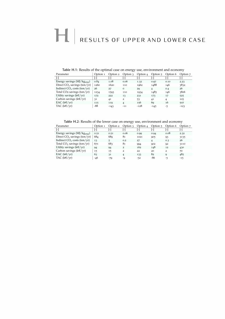
H R E S U LT S O F U P P E R A N D LO W E R C A S E
Table H.1: Results of the optimal case on energy use, environment and economyParameter Option 1 Option 2 Option 3 Option 4 Option 5 Option 6 Option 7
[-] [-] [-] [-] [-] [-] [-] [-]Energy savings (MJ/kgsmp) 0.84 1.08 0.06 1.32 0.97 0.10 2.23
Direct CO2 savings (ton/yr) 1260 1620 110 1962 1488 146 3832
Indirect CO2 costs (ton/yr) 26 27 0 29 4 0.4 26
Total CO2 savings (ton/yr) 1234 1593 110 1934 1485 146 3806
Utility savings (ke/yr) 172 222 13 231 173 17 525
Carbon savings (ke/yr) 31 41 2 53 41 4 105
EAC (ke/yr) 115 119 4 156 69 16 507
TAC (ke/yr) -88 -143 -11 -128 -145 -5 -123
Table H.2: Results of the lower case on energy use, environment and economyParameter Option 1 Option 2 Option 3 Option 4 Option 5 Option 6 Option 7
[-] [-] [-] [-] [-] [-] [-] [-]Energy savings (MJ/kgsmp) 0.51 0.51 0.06 0.99 0.94 0.08 2.32
Direct CO2 savings (ton/yr) 684 689 81 1021 905 93 3135
Indirect CO2 costs (ton/yr) 13 5 0.2 27 4 0.3 26
Total CO2 savings (ton/yr) 671 683 81 994 902 92 3110
Utility savings (ke/yr) 94 94 2 162 148 12 430
Carbon savings (ke/yr) 15 15 2 22 20 2 70
EAC (ke/yr) 63 31 4 133 82 9 485
TAC (ke/yr) -46 -79 -9 -52 -86 -5 -15

colophonThis document was typeset using LATEX. The document layout was generated usingthe arsclassica package by Lorenzo Pantieri, which is an adaption of the originalclassicthesis package from Andre Miede.