Validation of Xpatch Computer Models for Human Body … · Validation of Xpatch Computer Models for ... Validation of Xpatch Computer Models for Human Body Radar ... Xpatch as an

Validation of Xpatch Computer Models for Human Body

Radar Signature

by Traian Dogaru and Calvin Le

ARL-TR-4403 March 2008 Approved for public release; distribution unlimited.

NOTICES

Disclaimers The findings in this report are not to be construed as an official Department of the Army position unless so designated by other authorized documents. Citation of manufacturer’s or trade names does not constitute an official endorsement or approval of the use thereof. Destroy this report when it is no longer needed. Do not return it to the originator.

Army Research Laboratory Adelphi, MD 20783-1197

ARL-TR-4403 March 2008

Validation of Xpatch Computer Models for Human Body Radar Signature

Traian Dogaru and Calvin Le

Sensors and Electron Devices Directorate, ARL Approved for public release; distribution unlimited.

ii

REPORT DOCUMENTATION PAGE Form Approved OMB No. 0704-0188

Public reporting burden for this collection of information is estimated to average 1 hour per response, including the time for reviewing instructions, searching existing data sources, gathering and maintaining the data needed, and completing and reviewing the collection information. Send comments regarding this burden estimate or any other aspect of this collection of information, including suggestions for reducing the burden, to Department of Defense, Washington Headquarters Services, Directorate for Information Operations and Reports (0704-0188), 1215 Jefferson Davis Highway, Suite 1204, Arlington, VA 22202-4302. Respondents should be aware that notwithstanding any other provision of law, no person shall be subject to any penalty for failing to comply with a collection of information if it does not display a currently valid OMB control number. PLEASE DO NOT RETURN YOUR FORM TO THE ABOVE ADDRESS. 1. REPORT DATE (DD-MM-YYYY)

March 2008 2. REPORT TYPE

Final 3. DATES COVERED (From - To)

2005 to 2007 5a. CONTRACT NUMBER

5b. GRANT NUMBER

4. TITLE AND SUBTITLE

Validation of Xpatch Computer Models for Human Body Radar Signature

5c. PROGRAM ELEMENT NUMBER

5d. PROJECT NUMBER

5e. TASK NUMBER

6. AUTHOR(S)

Traian Dogaru and Calvin Le

5f. WORK UNIT NUMBER

7. PERFORMING ORGANIZATION NAME(S) AND ADDRESS(ES)

U.S. Army Research Laboratory ATTN: AMSRD ARL SE RU 2800 Powder Mill Road Adelphi, MD 20783-1197

8. PERFORMING ORGANIZATION REPORT NUMBER

ARL-TR-4403

10. SPONSOR/MONITOR'S ACRONYM(S)

9. SPONSORING/MONITORING AGENCY NAME(S) AND ADDRESS(ES)

11. SPONSOR/MONITOR'S REPORT NUMBER(S)

12. DISTRIBUTION/AVAILABILITY STATEMENT

Approved for public release; distribution unlimited.

13. SUPPLEMENTARY NOTES

14. ABSTRACT

This technical report compares the radar signatures of a human body as computed by the Finite Difference Time Domain (FDTD) and Xpatch modeling techniques. Our main purpose is to validate the Xpatch (approximate) models with an exact electromagnetic solver (FDTD). We achieve this by comparing the radar cross section (RCS), range profiles and synthetic aperture radar (SAR) images of the human body, as computed by the two methods. This work is important in validating Xpatch as an accurate tool for modeling general STTW radar scenarios, where a major goal consists in detecting and identifying humans enclosed in building structures.

15. SUBJECT TERMS

Radar signature, computational electromagnetics, human body

16. SECURITY CLASSIFICATION OF: 19a. NAME OF RESPONSIBLE PERSON

Traian Dogaru a. REPORT

U b. ABSTRACT

U c. THIS PAGE

U

17. LIMITATION OF ABSTRACT

SAR

18. NUMBER OF PAGES

28 19b. TELEPHONE NUMBER (Include area code)

301-394-1482 Standard Form 298 (Rev. 8/98) Prescribed by ANSI Std. Z39.18

iii

Contents

Lisa of Figures iv

Acknowledgments vii

1. Introduction 1

2. Modeling Techniques 2

3. Numerical Results 2 3.1. The Uniform Dielectric Model of a Human Body ..........................................................2

3.2. Human Body Radar Cross Section..................................................................................6

3.3. Human Body Radar Range Profiles ................................................................................9

3.4. Synthetic Aperture Images of a Human Body...............................................................12

4. Conclusions 14

5. References 16

Acronyms 17

Distribution List 18

iv

Lisa of Figures

Figure 1. Computational meshes for (a) the fat man model and (b) the fit man model................. 3 Figure 2. RCS comparison between the complete fat man body model and other simplified

human body models with identical exterior geometry, at 0° azimuth (front view) and 0° elevation, V-V polarization..................................................................................................... 4

Figure 3. RCS of the fat man body model with tissue dielectric constants computed at two different frequencies, at 0° azimuth (front view) and 0° elevation, V-V polarization........... 6

Figure 4. RCS of the fit man body model versus frequency as computed by FDTD and Xpatch, at 0° azimuth (front view) and 0° elevation, showing (a) V-V polarization and (b) H-H polarization. ............................................................................................................................ 7

Figure 5. RCS of the fit man body model versus azimuth angle as computed by FDTD and Xpatch, at 1 GHz and 0° elevation, showing (a) V-V polarization and (b) H-H polarization.8




Figure 9. Two walking snapshots of the fit man body model, as obtained by Maya software animation............................................................................................................................... 10

Figure 10. Range profiles of the fit man body model in figure 9a, as computed by FDTD (red line) and Xpatch (black line), at 0° elevation and V-V polarization for (a) 0° azimuth, (b) 30° azimuth, (c) 60° azimuth and (d) 90° azimuth. NOTE: a top view of the mesh (as seen by the radar) was overlaid onto the range profiles........................................................ 11

Figure 11. Range profiles of the fit man body model in figure 9b, as computed by FDTD (red line) and Xpatch (black line), at 0° elevation and V-V polarization for (a) 0° azimuth, (b) 30° azimuth, (c) 60° azimuth and (d) 90° azimuth. NOTE: a top view of the mesh (as seen by the radar) was overlaid onto the range profiles........................................................ 12

Figure 12. SAR image of the fit man (as shown in figure 1b), at 2 GHz center frequency, 3 GHz bandwidth, V-V polarization, with 400 aperture modulated by a Hanning window, showing (a) the image obtained by FDTD simulations and (b) the image obtained by Xpatch simulations. NOTES: The down-range is along the y axis, whereas the cross-range is along the x axis, with distance units in meters; the pixel intensities (in dB) are mapped onto a pseudocolor scale. ................................................................................................................. 13

v

Figure 13. SAR image of the fit man (as shown in figure 1b), at 2 GHz center frequency, 3 GHz bandwidth, H-H polarization, with 400 aperture modulated by a Hanning window, showing (a) the image obtained by FDTD simulations and (b) the image obtained by Xpatch simulations. NOTES: The down-range is along the y axis, whereas the cross-range is along the x axis, with distance units in meters; the pixel intensities (in dB) are mapped onto a pseudocolor scale. ................................................................................................................. 14

vi

INTENTIONALLY LEFT BLANK.

vii

Acknowledgments

This study was partially funded by the Communications-Electronics Research Development and Engineering Center (CERDEC), Intelligence and Information Warfare Directorate (I2WD) at Ft. Monmouth, NJ. The synthetic aperture radar images in section 3.4 were created by Lam Nguyen.

viii

INTENTIONALLY LEFT BLANK.

1

1. Introduction

The radar signature of the human body is currently a research topic of great interest to defense agencies. The detection, identification and tracking of humans constitute essential components of sensor systems operating in a battlefield environment characterized by asymmetric threats. The low-frequency ultra-wideband (UWB) radar has proved great potential for detecting concealed targets, such as in foliage penetration (FOPEN) or sensing through the wall (STTW) scenarios. For all these applications, operating the radar in the low frequency microwave range (200 MHz to 3 GHz) has the advantage of good penetration through both natural and man-made structures that conceal the target.

In previous studies (1,2), we investigated the radar signature of the human body from a computer modeling perspective. In that work, we used two different modeling techniques: the Finite Difference Time Domain (FDTD) and Xpatch. All the radar modeling at low frequencies (under 3 GHz) was performed with FDTD, which is an exact electromagnetic (EM) solver. Xpatch was only used for high-frequency models (Ku- and Ka-bands [2]), since that code employs modeling techniques that work better in that regime. However, there is great interest in applying Xpatch modeling to many low-frequency radar problems, such as STTW scenarios. The main reason is that, although accurate, the FDTD algorithm is very computationally intensive. In consequence, trying to model geometries involving large rooms and building structures may become prohibitive for an FDTD code, even when large High Performance Computing (HPC) systems are available. On the other hand, Xpatch can achieve vastly superior speed in modeling radar problems (typically 100 to 1000 times faster) compared to FDTD, while using significantly less memory. Nevertheless, before we can confidently apply Xpatch to these low frequency scenarios, we need to understand its accuracy and limitations. This study performs a comparison between Xpatch and FDTD for human body radar signature prediction and represents an important step in validating Xpatch as an efficient and accurate tool for complex STTW radar problems.

This report is organized as follows. We start by presenting a short overview of the modeling methods used in this study (section 2). The modeling results are presented in section 3. We first discuss the uniform dielectric model of the human body for radar signature prediction in section 3.1. We then compare the FDTD and Xpatch simulation results on the human body radar return, as radar cross section (RCS) in section 3.2, radar range profiles in section 3.3, and synthetic aperture radar (SAR) images in section 3.4. We finalize with conclusions in section 4.

2

2. Modeling Techniques

For this study we employ two widely used computational electromagnetics (CEM) modeling techniques, namely FDTD and ray-tracing combined with physical optics (PO). The FDTD implementation we used for this work is called AFDTD and was entirely developed at the U.S. Army Research Laboratory (ARL) for radar signature modeling. We also used Xpatch (4), which is a ray-tracing-based code, developed by Science Applications International Corporation (SAIC) under a grant from the U.S. Air Force. Since these codes were presented in previous reports (1 through 3), we refer the reader to that work. Also, a number of excellent books treat these CEM modeling techniques in detail (5 through 7).

The main purpose of this investigation is to validate the Xpatch models of the human body radar signature by comparing these results with FDTD simulations. A detailed account of the human body radar signature as computed by FDTD was given in (1), including a code validation for this type of problems by a completely independent CEM technique. The FDTD method accuracy is not surprising, given the fact that it has been the method of choice in most modeling studies involving the interaction of EM fields with the human body. However, it is not clear whether Xpatch can be successfully applied to the same type of problems, especially in a relatively low frequency band (1-5 GHz), where most STTW radars operate. As a reminder, Xpatch implements a ray tracing technique combined with PO (7) (both approximate EM field computation methods), which work more accurately at high frequencies (when the wavelength is much smaller than the target size). Limitations of the Xpatch code include: PO errors for scattering at angles off the specular direction, and the inability to account for diffraction from dielectric wedges, surface, creeping, or traveling waves. Since these issues can become important for low frequencies and relatively small target sizes, we need to investigate how accurately Xpatch can predict the human body radar signature before we can apply this code to more complex STTW radar scenarios.

We have performed the simulations in this study at the U.S. Army Major Shared Resource Center (MSRC) (8) on Linux Networx Evolocity II clusters. All the graphics in this report were done with MATLAB. The pre- and post-processing were performed on Dell workstations running Windows XP.

3. Numerical Results

3.1. The Uniform Dielectric Model of a Human Body

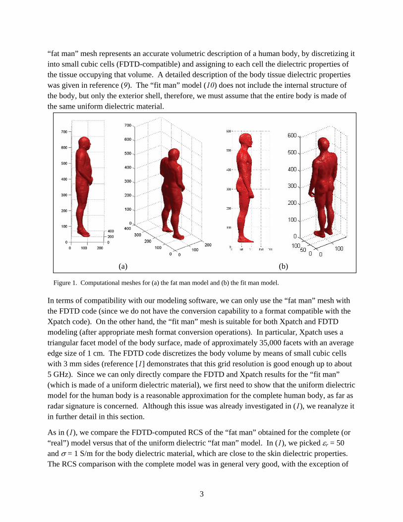
In reference (1) we performed a detailed analysis of the human body RCS. For that modeling work, we used two different body meshes, called the “fat man” and the “fit man” (figure 1). The

3

“fat man” mesh represents an accurate volumetric description of a human body, by discretizing it into small cubic cells (FDTD-compatible) and assigning to each cell the dielectric properties of the tissue occupying that volume. A detailed description of the body tissue dielectric properties was given in reference (9). The “fit man” model (10) does not include the internal structure of the body, but only the exterior shell, therefore, we must assume that the entire body is made of the same uniform dielectric material.

(a) (b)

Figure 1. Computational meshes for (a) the fat man model and (b) the fit man model.

In terms of compatibility with our modeling software, we can only use the “fat man” mesh with the FDTD code (since we do not have the conversion capability to a format compatible with the Xpatch code). On the other hand, the “fit man” mesh is suitable for both Xpatch and FDTD modeling (after appropriate mesh format conversion operations). In particular, Xpatch uses a triangular facet model of the body surface, made of approximately 35,000 facets with an average edge size of 1 cm. The FDTD code discretizes the body volume by means of small cubic cells with 3 mm sides (reference [1] demonstrates that this grid resolution is good enough up to about 5 GHz). Since we can only directly compare the FDTD and Xpatch results for the “fit man” (which is made of a uniform dielectric material), we first need to show that the uniform dielectric model for the human body is a reasonable approximation for the complete human body, as far as radar signature is concerned. Although this issue was already investigated in (1), we reanalyze it in further detail in this section.

As in (1), we compare the FDTD-computed RCS of the “fat man” obtained for the complete (or “real”) model versus that of the uniform dielectric “fat man” model. In (1), we picked εr = 50 and σ = 1 S/m for the body dielectric material, which are close to the skin dielectric properties. The RCS comparison with the complete model was in general very good, with the exception of

4

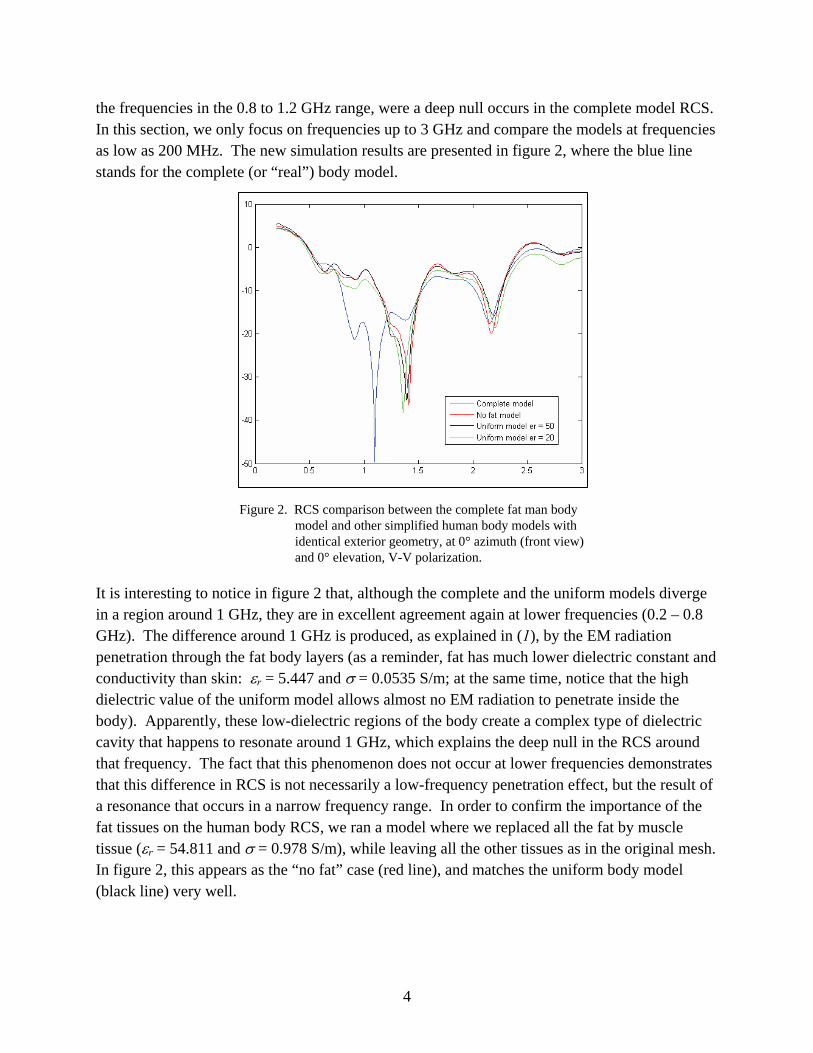
the frequencies in the 0.8 to 1.2 GHz range, were a deep null occurs in the complete model RCS. In this section, we only focus on frequencies up to 3 GHz and compare the models at frequencies as low as 200 MHz. The new simulation results are presented in figure 2, where the blue line stands for the complete (or “real”) body model.

Figure 2. RCS comparison between the complete fat man body model and other simplified human body models with identical exterior geometry, at 0° azimuth (front view) and 0° elevation, V-V polarization.

It is interesting to notice in figure 2 that, although the complete and the uniform models diverge in a region around 1 GHz, they are in excellent agreement again at lower frequencies (0.2 – 0.8 GHz). The difference around 1 GHz is produced, as explained in (1), by the EM radiation penetration through the fat body layers (as a reminder, fat has much lower dielectric constant and conductivity than skin: εr = 5.447 and σ = 0.0535 S/m; at the same time, notice that the high dielectric value of the uniform model allows almost no EM radiation to penetrate inside the body). Apparently, these low-dielectric regions of the body create a complex type of dielectric cavity that happens to resonate around 1 GHz, which explains the deep null in the RCS around that frequency. The fact that this phenomenon does not occur at lower frequencies demonstrates that this difference in RCS is not necessarily a low-frequency penetration effect, but the result of a resonance that occurs in a narrow frequency range. In order to confirm the importance of the fat tissues on the human body RCS, we ran a model where we replaced all the fat by muscle tissue (εr = 54.811 and σ = 0.978 S/m), while leaving all the other tissues as in the original mesh. In figure 2, this appears as the “no fat” case (red line), and matches the uniform body model (black line) very well.

5

This result underscores the importance of the fat body layers on the human radar signature at certain frequencies. We infer that a different body size with different fat content may resonate at different frequencies than our “fat man” model. In fact, a body that contains very little fat (such as the “fit man”) should produce a radar signature much closer to the “no fat” case in figure 2. Therefore, we think that the complete “fat man” model (with its body type particularities) is not entirely representative for our modeling work on STTW scenarios. In this context, an “all muscle fit man” (such as the uniform dielectric model that we consider in this report) should be at least as representative as the “fat man” in our scenarios of interest.

Since the dielectric constant of 50 that we picked for the uniform body model seems somewhat arbitrary, we tried other values (both for the dielectric constant and the conductivity) and compared the RCS in the same frequency range. For values as low as εr = 20 and σ = 0.5 S/m (green line in figure 2), we noticed very little difference among the various uniform dielectric models. This is easy to explain by the fact that a dielectric material with high εr and σ (such as in our models) reflects the EM radiation almost entirely, allowing very little penetration inside the structure. In fact, we obtained fairly similar results for a human body made entirely of perfect electric conductor (PEC) (however, in that case, surface waves are excited along the body (7), producing some deviations from the high dielectric constant, high loss material model, which does not support surface wave phenomena). The conclusion is that, as long as we pick large dielectric constant and conductivity for the human body material, the RCS is not very sensitive to their particular values.

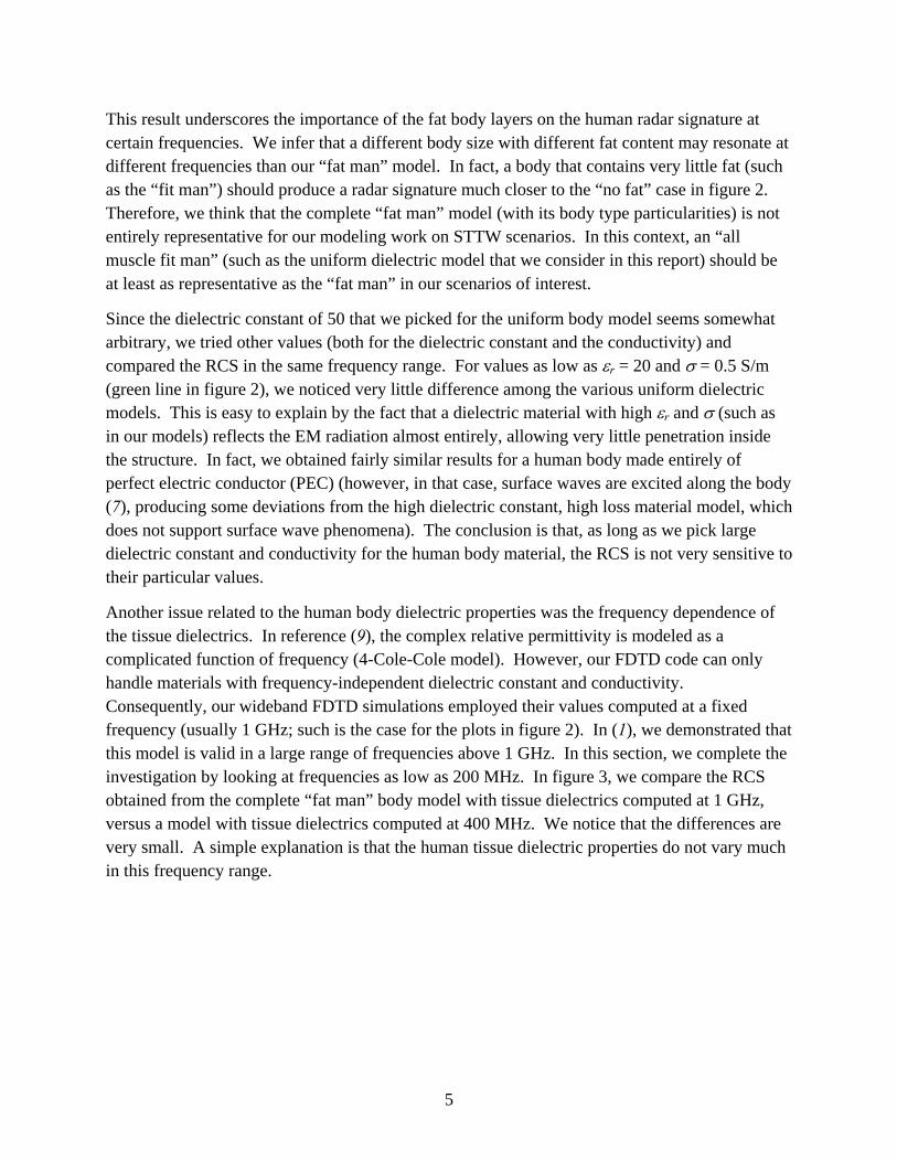
Another issue related to the human body dielectric properties was the frequency dependence of the tissue dielectrics. In reference (9), the complex relative permittivity is modeled as a complicated function of frequency (4-Cole-Cole model). However, our FDTD code can only handle materials with frequency-independent dielectric constant and conductivity. Consequently, our wideband FDTD simulations employed their values computed at a fixed frequency (usually 1 GHz; such is the case for the plots in figure 2). In (1), we demonstrated that this model is valid in a large range of frequencies above 1 GHz. In this section, we complete the investigation by looking at frequencies as low as 200 MHz. In figure 3, we compare the RCS obtained from the complete “fat man” body model with tissue dielectrics computed at 1 GHz, versus a model with tissue dielectrics computed at 400 MHz. We notice that the differences are very small. A simple explanation is that the human tissue dielectric properties do not vary much in this frequency range.

6

Figure 3. RCS of the fat man body model with tissue dielectric constants computed at two different frequencies, at 0° azimuth (front view) and 0° elevation, V-V polarization.

To complete the analysis we mention that, although the results presented here were obtained for vertical-vertical (V-V) polarization and front incidence (0° azimuth), similar results were obtained for horizontal-horizontal (H-H) polarization and other aspect angles. We conclude that the uniform dielectric human body model with εr = 50 and σ = 1 S/m is representative for RCS modeling in a large range of frequencies (from 200 MHz up to at least 9 GHz), especially for a body type such as the “fit man”. Certain particular body types (such as the “fat man”) may present specific deviations from this model (related, for instance, to the fat body layers); however, we think that these deviations are not necessarily representative for all body types.

3.2. Human Body Radar Cross Section

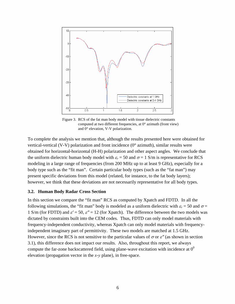
In this section we compare the “fit man” RCS as computed by Xpatch and FDTD. In all the following simulations, the “fit man” body is modeled as a uniform dielectric with εr = 50 and σ = 1 S/m (for FDTD) and ε′ = 50, ε″ = 12 (for Xpatch). The difference between the two models was dictated by constraints built into the CEM codes. Thus, FDTD can only model materials with frequency-independent conductivity, whereas Xpatch can only model materials with frequency-independent imaginary part of permittivity. These two models are matched at 1.5 GHz. However, since the RCS is not sensitive to the particular values of σ or ε″ (as shown in section 3.1), this difference does not impact our results. Also, throughout this report, we always compute the far-zone backscattered field, using plane-wave excitation with incidence at 00 elevation (propagation vector in the x-y plane), in free-space.

7

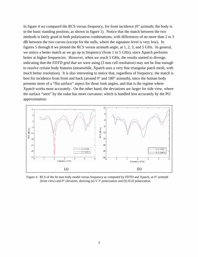
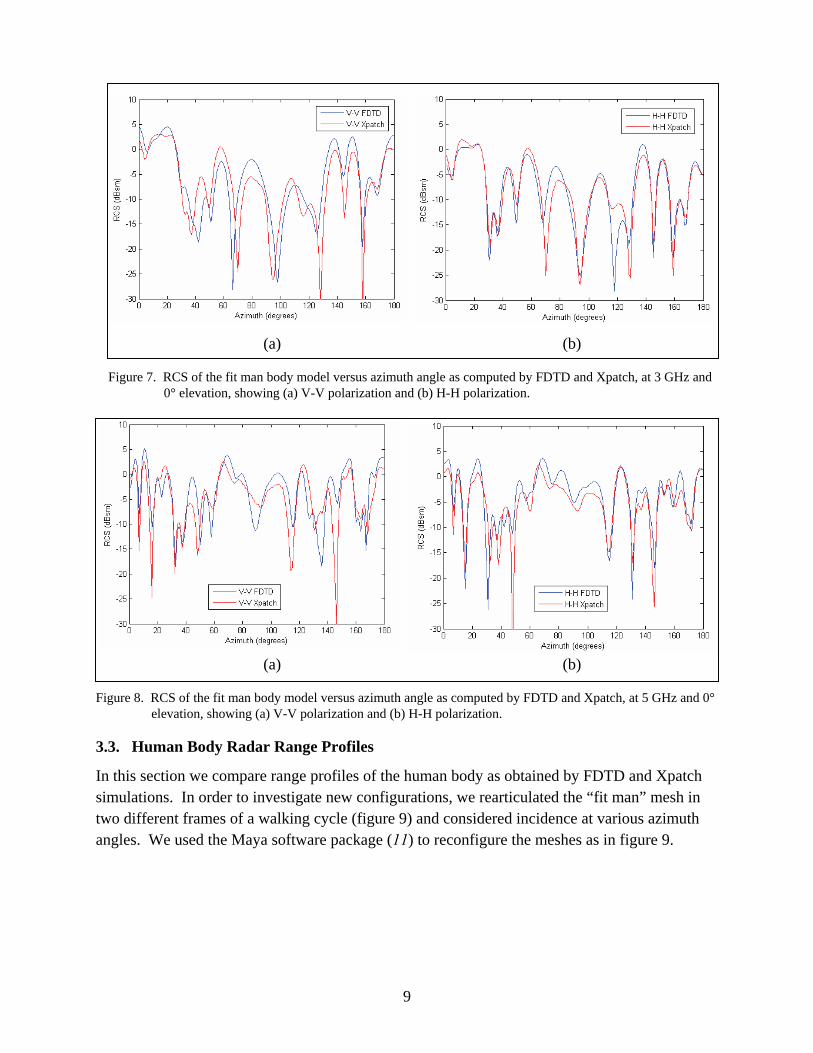
In figure 4 we compared the RCS versus frequency, for front incidence (0° azimuth; the body is in the basic standing position, as shown in figure 1). Notice that the match between the two methods is fairly good in both polarization combinations, with differences of no more than 2 to 3 dB between the two curves (except for the nulls, where the signature level is very low). In figures 5 through 8 we plotted the RCS versus azimuth angle, at 1, 2, 3, and 5 GHz. In general, we notice a better match as we go up in frequency (from 1 to 5 GHz), since Xpatch performs better at higher frequencies. However, when we reach 5 GHz, the results started to diverge, indicating that the FDTD grid that we were using (3 mm cell resolution) may not be fine enough to resolve certain body features (meanwhile, Xpatch uses a very fine triangular patch mesh, with much better resolution). It is also interesting to notice that, regardless of frequency, the match is best for incidence from front and back (around 0° and 180° azimuth), since the human body presents more of a “flat surface” aspect for those look angles, and that is the regime where Xpatch works most accurately. On the other hand, the deviations are larger for side view, where the surface “seen” by the radar has more curvature, which is handled less accurately by the PO approximation.

(a) (b)

Figure 4. RCS of the fit man body model versus frequency as computed by FDTD and Xpatch, at 0° azimuth (front view) and 0° elevation, showing (a) V-V polarization and (b) H-H polarization.

8

(a) (b)

Figure 5. RCS of the fit man body model versus azimuth angle as computed by FDTD and Xpatch, at 1 GHz and 0° elevation, showing (a) V-V polarization and (b) H-H polarization.

(a) (b)


9

(a) (b)


(a) (b)


3.3. Human Body Radar Range Profiles

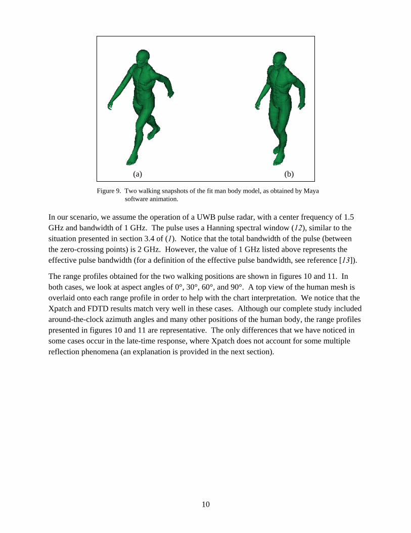
In this section we compare range profiles of the human body as obtained by FDTD and Xpatch simulations. In order to investigate new configurations, we rearticulated the “fit man” mesh in two different frames of a walking cycle (figure 9) and considered incidence at various azimuth angles. We used the Maya software package (11) to reconfigure the meshes as in figure 9.

10

(a) (b)

Figure 9. Two walking snapshots of the fit man body model, as obtained by Maya software animation.

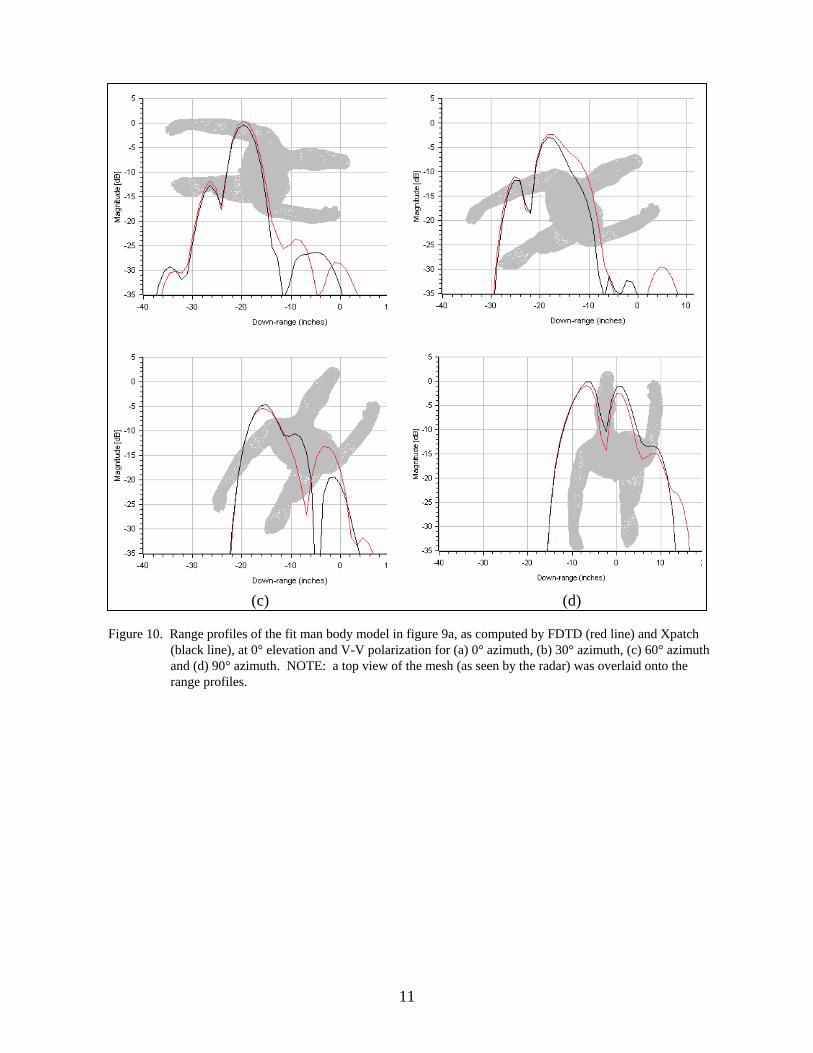
In our scenario, we assume the operation of a UWB pulse radar, with a center frequency of 1.5 GHz and bandwidth of 1 GHz. The pulse uses a Hanning spectral window (12), similar to the situation presented in section 3.4 of (1). Notice that the total bandwidth of the pulse (between the zero-crossing points) is 2 GHz. However, the value of 1 GHz listed above represents the effective pulse bandwidth (for a definition of the effective pulse bandwidth, see reference [13]).

The range profiles obtained for the two walking positions are shown in figures 10 and 11. In both cases, we look at aspect angles of 0°, 30°, 60°, and 90°. A top view of the human mesh is overlaid onto each range profile in order to help with the chart interpretation. We notice that the Xpatch and FDTD results match very well in these cases. Although our complete study included around-the-clock azimuth angles and many other positions of the human body, the range profiles presented in figures 10 and 11 are representative. The only differences that we have noticed in some cases occur in the late-time response, where Xpatch does not account for some multiple reflection phenomena (an explanation is provided in the next section).

11

(a) (b) (c) (d)

Figure 10. Range profiles of the fit man body model in figure 9a, as computed by FDTD (red line) and Xpatch (black line), at 0° elevation and V-V polarization for (a) 0° azimuth, (b) 30° azimuth, (c) 60° azimuth and (d) 90° azimuth. NOTE: a top view of the mesh (as seen by the radar) was overlaid onto the range profiles.

12

(a) (b) (c) (d)

Figure 11. Range profiles of the fit man body model in figure 9b, as computed by FDTD (red line) and Xpatch (black line), at 0° elevation and V-V polarization for (a) 0° azimuth, (b) 30° azimuth, (c) 60° azimuth and (d) 90° azimuth. NOTE: a top view of the mesh (as seen by the radar) was overlaid onto the range profiles.

3.4. Synthetic Aperture Images of a Human Body

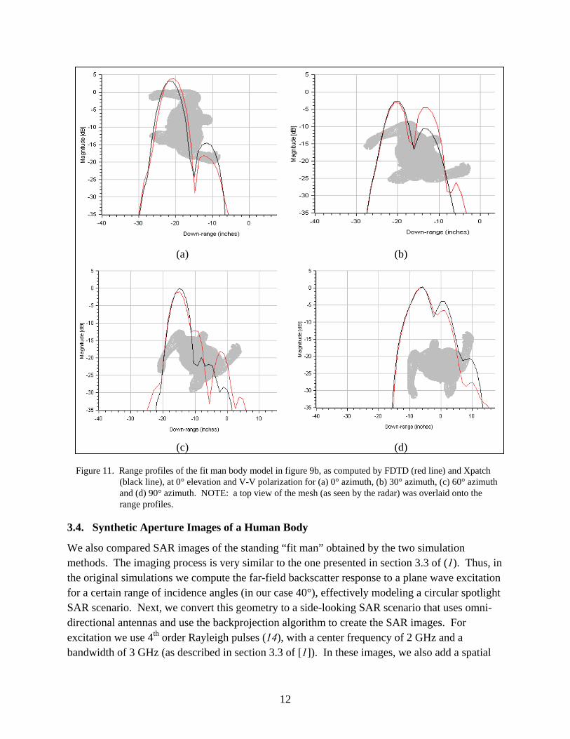
We also compared SAR images of the standing “fit man” obtained by the two simulation methods. The imaging process is very similar to the one presented in section 3.3 of (1). Thus, in the original simulations we compute the far-field backscatter response to a plane wave excitation for a certain range of incidence angles (in our case 40°), effectively modeling a circular spotlight SAR scenario. Next, we convert this geometry to a side-looking SAR scenario that uses omni-directional antennas and use the backprojection algorithm to create the SAR images. For excitation we use 4th order Rayleigh pulses (14), with a center frequency of 2 GHz and a bandwidth of 3 GHz (as described in section 3.3 of [1]). In these images, we also add a spatial

13

Hanning window taper to the contribution of each point on the aperture (equivalent to a window in the angular domain), in order to reduce the sidelobes (this procedure also reduces the cross-range resolution as compared to a no-window scenario).

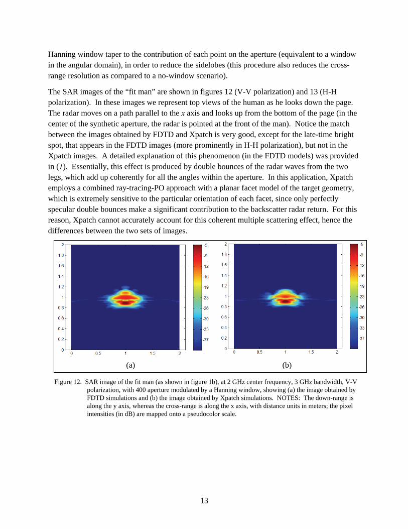
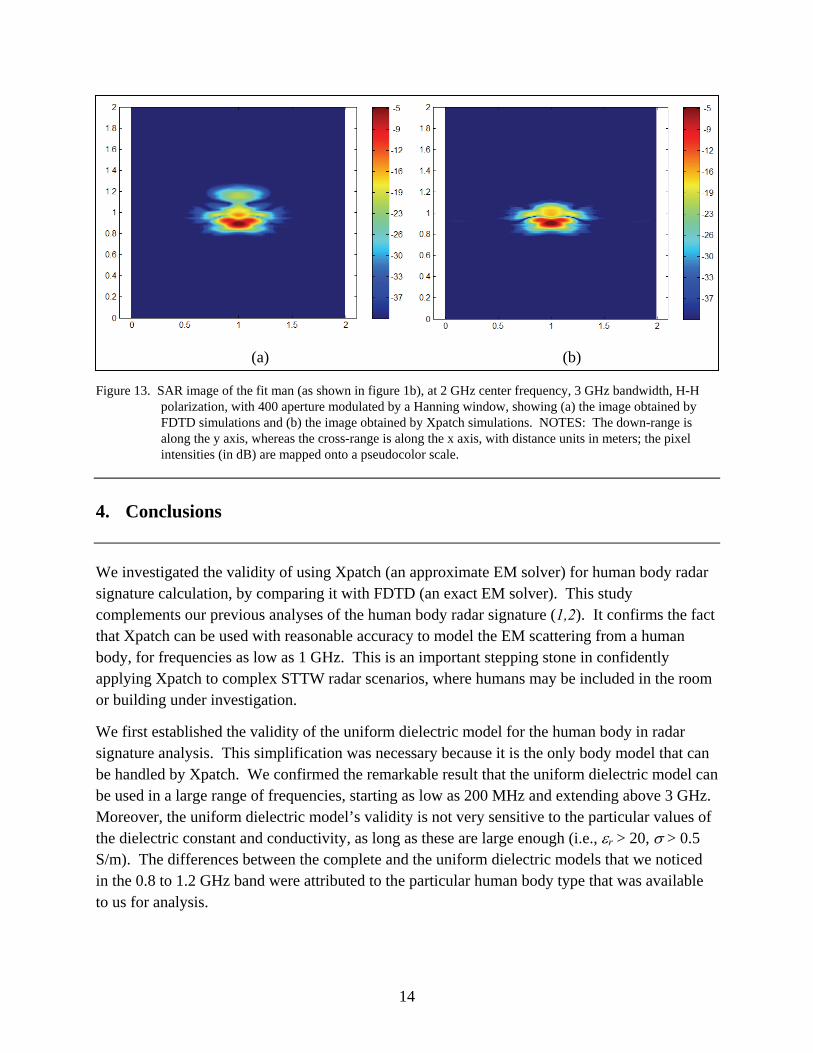
The SAR images of the “fit man” are shown in figures 12 (V-V polarization) and 13 (H-H polarization). In these images we represent top views of the human as he looks down the page. The radar moves on a path parallel to the x axis and looks up from the bottom of the page (in the center of the synthetic aperture, the radar is pointed at the front of the man). Notice the match between the images obtained by FDTD and Xpatch is very good, except for the late-time bright spot, that appears in the FDTD images (more prominently in H-H polarization), but not in the Xpatch images. A detailed explanation of this phenomenon (in the FDTD models) was provided in (1). Essentially, this effect is produced by double bounces of the radar waves from the two legs, which add up coherently for all the angles within the aperture. In this application, Xpatch employs a combined ray-tracing-PO approach with a planar facet model of the target geometry, which is extremely sensitive to the particular orientation of each facet, since only perfectly specular double bounces make a significant contribution to the backscatter radar return. For this reason, Xpatch cannot accurately account for this coherent multiple scattering effect, hence the differences between the two sets of images.

(a) (b)

Figure 12. SAR image of the fit man (as shown in figure 1b), at 2 GHz center frequency, 3 GHz bandwidth, V-V polarization, with 400 aperture modulated by a Hanning window, showing (a) the image obtained by FDTD simulations and (b) the image obtained by Xpatch simulations. NOTES: The down-range is along the y axis, whereas the cross-range is along the x axis, with distance units in meters; the pixel intensities (in dB) are mapped onto a pseudocolor scale.

14

(a) (b)

Figure 13. SAR image of the fit man (as shown in figure 1b), at 2 GHz center frequency, 3 GHz bandwidth, H-H polarization, with 400 aperture modulated by a Hanning window, showing (a) the image obtained by FDTD simulations and (b) the image obtained by Xpatch simulations. NOTES: The down-range is along the y axis, whereas the cross-range is along the x axis, with distance units in meters; the pixel intensities (in dB) are mapped onto a pseudocolor scale.

4. Conclusions

We investigated the validity of using Xpatch (an approximate EM solver) for human body radar signature calculation, by comparing it with FDTD (an exact EM solver). This study complements our previous analyses of the human body radar signature (1,2). It confirms the fact that Xpatch can be used with reasonable accuracy to model the EM scattering from a human body, for frequencies as low as 1 GHz. This is an important stepping stone in confidently applying Xpatch to complex STTW radar scenarios, where humans may be included in the room or building under investigation.

We first established the validity of the uniform dielectric model for the human body in radar signature analysis. This simplification was necessary because it is the only body model that can be handled by Xpatch. We confirmed the remarkable result that the uniform dielectric model can be used in a large range of frequencies, starting as low as 200 MHz and extending above 3 GHz. Moreover, the uniform dielectric model’s validity is not very sensitive to the particular values of the dielectric constant and conductivity, as long as these are large enough (i.e., εr > 20, σ > 0.5 S/m). The differences between the complete and the uniform dielectric models that we noticed in the 0.8 to 1.2 GHz band were attributed to the particular human body type that was available to us for analysis.

15

Next, we compared the “fit man” radar signature as computed by FDTD and Xpatch and presented under various formats. We analyzed the RCS versus frequency at a given aspect angle, and the RCS versus azimuth angle at particular frequencies. We also looked at the range profiles obtained for the “fit man” in various walking positions for a UWB radar excitation. Finally, we created SAR images from the UWB scattering data obtained for a wide range of aspect angles. In all cases, the match between the two modeling methods was surprisingly good, given the expected Xpatch limitations in the low frequency regime. These results increase our confidence in Xpatch as an indispensable tool for modeling complex STTW radar scenarios, where a major goal consists in detecting and identifying humans enclosed in building structures.

16

5. References

1. Dogaru, T.; Nguyen, L.; Le, C. Computer Models of the Human Body Signature for Sensing Through the Wall Radar Applications; ARL-TR-4290; U.S. Army Research Laboratory: Adelphi, MD, September 2007.

2. Le, C.; Dogaru, T. Numerical Modeling of the Airborne Radar Signature of Dismount Personnel in the UHF-, L-, Ku- and Ka-Bands; ARL-TR-4336; U.S. Army Research Laboratory: Adelphi, MD, December 2008.

3. Dogaru, T.; Le, C. Xpatch and Finite-Difference Time-Domain Modeling of the M1 Tank Radar Signature in the L-band; ARL-TR-4291; U.S. Army Research Laboratory: Adelphi, MD, September 2007.

4. XPATCH User’s Manual, SAIC/DEMACO, Champaign, IL. (This document is export controlled, available to U.S. Government users and DoD Contractors only).

5. Taflove, A.; Hagness, S. C. Computational Electrodynamics: The Finite-Difference Time-Domain, Artech House, Boston, MA, 2000.

6. Kunz, K.; Luebbers, R. The Finite-Difference Time-Domain Method for Electromagnetics, CRC Press, Boca Raton, FL, 1993.

7. Knott E.; Shaeffer J.; Tuley, M. Radar Cross Section, Artech House, Boston, MA, 1993.

8. ARL MSRC Web page: http://www.arl.hpc.mil (accessed August 2007).

9. Gabriel, C. Compilation of the dielectric properties of body tissue at RF and microwave frequencies. USAF School Aerospace Med., Brooks AFB, TX, AL/OE-TR-1996-0037, 1996.

10. 3D CAD Browser Web page: http://3dcadbrowser.com (accessed July 2005).

11. Autodesk Web page. http://www.autodesk.com/maya (accessed June 2007).

12. Oppenheim, A. V.; Schafer, R. W. Discrete-Time Signal Processing, Prentice Hall, Englewood Cliffs, NJ, 1989.

13. Shaeffer, J. F.; Hom, K. W.; Baucke, R. C.; Cooper, B. A.; Talcott, N. A. Bistatic k-space imaging for electromagnetic prediction codes for scattering and antennas; Technical Paper NASA-TP-3569; National Aeronautics and Space Administration: Langley, VA, July 1996.

14. Hubral P.; Tygel, M. Analysis of the Rayleigh pulse. Geophysics 1989, 54, 654–658.

17

Acronyms

ARL U.S. Army Research Laboratory

CEM computational electromagnetics

CERDEC Communications-Electronics Research Development and Engineering Center

EM electromagnetic

FDTD Finite Difference Time Domain

FOPEN foliage penetration

H-H horizontal-horizontal

HPC High-Performance Computing

I2WD Intelligence and Information Warfare Directorate

MSRC Major Shared Resource Center

PEC perfect electric conductor

PO physical optics

RCS radar cross section

SAIC Science Applications International Corporation

SAR synthetic aperture radar

STTW sensing through the wall

UWB ultra-wideband

V-V vertical-vertical

18

Distribution List

No. of Copies Organization 1 ADMNSTR PDF DEFNS TECHL INFO CTR ATTN DTIC OCP (ELECTRONIC COPY) 8725 JOHN J KINGMAN RD STE 0944 FT BELVOIR VA 22060-6218

1 DARPA ATTN IXO S WELBY 3701 N FAIRFAX DR ARLINGTON VA 22203-1714

1 OFC OF THE SECY OF DEFNS ATTN ODDRE (R&AT) THE PENTAGON WASHINGTON DC 20301-3080

1 US ARMY RSRCH DEV & ENGRG CMND ARMAMENT RSRCH DEV & ENGRG CTR ARMAMENT ENGRG & TECHNLGY CTR ATTN AMSRD AAR AEF T J MATTS BLDG 305 APG MD 21005-500 1 US ARMY TRADOC BATTLE LAB INTEGRATION & TECHL DIRCTRT ATTN ATCD B 10 WHISTLER LANE FT MONROE VA 23651-5850

2 US ARMY RDECOM CERDEC I2WD ATTN AMSRD CER IW IM W CHIN BLDG 600 MCAFEE CENTER FT MONMOUTH NJ 07703

1 PM TIMS PROFILER (MMS P) AN/TMQ 52 ATTN B GRIFFIES BUILDING 563 FT MONMOUTH NJ 07703

1 US ARMY INFO SYS ENGRG CMND ATTN AMSEL IE TD F JENIA FT HUACHUCA AZ 85613-5300

1 COMMANDER US ARMY RDECOM ATTN AMSRD AMR W C MCCORKLE 5400 FOWLER RD REDSTONE ARSENAL AL 35898-5000

No. of Copies Organization 1 US ARMY RSRCH LAB ATTN AMSRD ARL CI OK TP TECHL LIB T LANDFRIED BLDG 4600 APG MD 21005-5066 1 US GOVERNMENT PRINT OFF DEPOSITORY RECEIVING SECTION ATTN MAIL STOP IDAD J TATE 732 NORTH CAPITOL ST NW WASHINGTON DC 20402

1 DIRECTOR US ARMY RSRCH LAB ATTN AMSRD ARL RO EV W D BACH PO BOX 12211 RESEARCH TRIANGLE PARK NC 27709

12 US ARMY RSRCH LAB ATTN AMSRD ARL CI OK T TECHL PUB ATTN AMSRD ARL CI OK TL TECHL LIB ATTN AMSRD ARL SE RM W O COBURN ATTN AMSRD ARL SE RU A SULLIVAN ATTN AMSRD ARL SE RU C LE ATTN AMSRD ARL SE RU G GAUNAURD ATTN AMSRD ARL SE RU J SICHINA ATTN AMSRD ARL SE RU K KAPPRA ATTN AMSRD ARL SE RU M RESSLER ATTN AMSRD ARL SE RU T DOGARU (2 COPIES) ATTN IMNE ALC IMS MAIL & RECORDS MGMT ADELPHI MD 20783-1197

25 TOTAL (1 elec, 24 hard copies)

Documents

Validation of Xpatch Computer Models for Human Body … · Validation of Xpatch Computer Models for ... Validation of Xpatch Computer Models for Human Body Radar ... Xpatch as an