Validation of three on-line flow simulations for injection molding

Validation of Three On-Line Flow Simulations forInjection Molding

David O. Kazmer, Ranjan Nageri, Vijay KudchakarDepartment of Plastics Engineering, University of Massachusetts Lowell, Lowell, Massachusetts 01854

Bingfeng FanDelphi Research Labs, 51786 Shelby Parkway, Shelby Township, Michigan 48315

Robert GaoDepartment of Mechanical and Industrial Engineering, Engineering Laboratory Building,University of Massachusetts Amherst, Amherst, Massachusetts 01003

Polymer process control is limited by a lack of observabil-ity of the distributed and transient polymer states. Threesimulations of varying complexity are validated for on-linesimulation of an injection molding process with a two drophot runner system to predict the state of the polymer meltin real time and thereby improve product quality in situ. Thesimplest simulation is a Newtonian model, which predictsflow rates given the inlet and outlet pressures. An interme-diate non-Newtonian and nonisothermal simulation utilizesa modified Ellis model that expresses the viscosity as afunction of the shear stress in which the modeling of theheat transfer utilizes a Bessel series expansion to includeeffects of heat conduction, heat convection, and internalshear heating. A numerical simulation was also developedthat utilizes a hybrid finite difference and finite elementscheme to simultaneously solve the mass, momentum,and heat equations. Numerical verification indicates thatthe flow rate predictions of the described simulationscompare well with the results from a commercial moldfilling simulation. However, empirical validation utilizing adesign of experiments indicates that the described analy-ses are qualitatively useful, but do not possess sufficientaccuracy for quantitative process and quality control. Spe-cifically, off-line validation using optimal transducer cali-bration with well characterized materials provided a coef-ficient of regression, R2, of �0.8. However, blind validationwith previously untested materials and no transducer re-calibration provided a regression coefficient of �0.4. While

the direction of the main effects was usually correct, themagnitudes of the effects were frequently outside the con-fidence interval of the observed behavior. Several sourcesof variance are discussed, including sensor calibration,constitutive modeling of the polymer melt, and numericalanalysis. POLYM. ENG. SCI., 46:274–288, 2006. © 2006 Society ofPlastics Engineers

INTRODUCTION

A fundamental difficulty in injection molding and otherdynamic polymer processing operations is the lack of ob-servability and controllability of the polymer melt. Becauseof the presence of an opaque and rigid steel mold to confinethe melt, it is not normally possible to “see” the state of themelt as it is formed during the process. This lack of observ-ability precludes the direct control of the melt flow duringpolymer processing. Accordingly, it would be a significantadvancement if process controllers could utilize simulationsin real time to estimate and control unobservable processstates (such as flow rate, shear stress, and other polymerstates) from other available process data. If successfullydeveloped and validated, such on-line simulations couldimprove the control of polymer processing to automaticallyadjust for external variations (such as material or environ-ment changes), maximize the quality to cost ratio of theprocess, and assist the operator in diagnosing and correctingthe root sources of defects.

Sophisticated numerical simulations have been devel-oped to model the non-Newtonian, nonisothermal flow inpolymer processing [1–4]. These simulations often utilizethe finite element method to model the flow conductanceacross the domain, and the finite difference method toestimate the shear rate and temperature distribution throughthe thickness. The flow conductance of each element in the

This work does not represent the opinions of Mold-Masters, the NationalScience Foundation, nor the United States government.Correspondence to: David O. Kazmer; e-mail: [email protected] grant sponsor: Mold-Masters Ltd.; contract grant sponsor: Man-ufacturing Machines and Equipment Program of the National ScienceFoundation; contract grant number: DMI-0428669.DOI 10.1002/pen.20463Publishedonline inWileyInterScience (www.interscience.wiley.com).© 2006 Society of Plastics Engineers

POLYMER ENGINEERING AND SCIENCE—2006

domain is typically estimated through the integration of themass and momentum equations across the thickness withrespect to the non-Newtonian viscosity. While advances inflow modeling, numerical methods, and computer technol-ogy have reduced computational times, numerical simula-tions require extended processing times compared with thesweep times of most process controllers. Accordingly, sim-ulations have not been incorporated into process controllers.

This research is directed to providing real time estimatesof melt flow rates and pressures at varying locations in aninjection mold given the feedback of the melt pressures inthe mold during the molding cycle. This approach can alsobe used to provide estimates of the output part weight, inputmelt viscosity, and other measures related to process con-sistency. To assess the feasibility of on-line simulationtechnology, several simulations of varying complexity havebeen developed and validated.

ANALYSIS

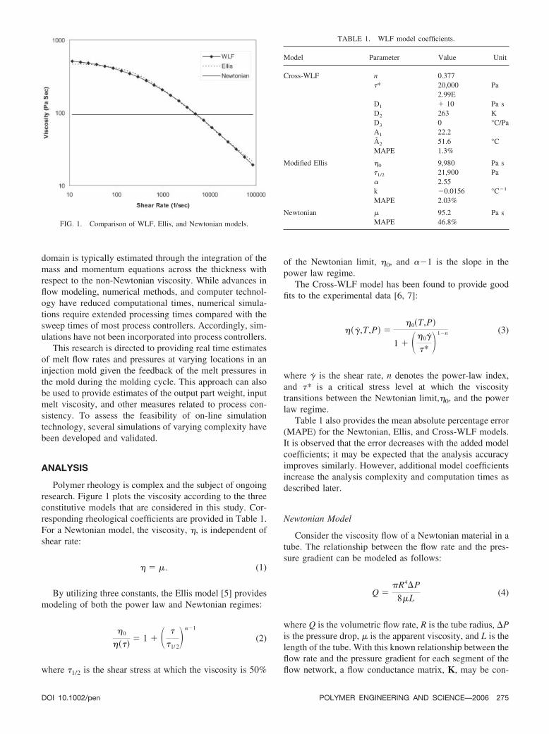
Polymer rheology is complex and the subject of ongoingresearch. Figure 1 plots the viscosity according to the threeconstitutive models that are considered in this study. Cor-responding rheological coefficients are provided in Table 1.For a Newtonian model, the viscosity, �, is independent ofshear rate:

� � �. (1)

By utilizing three constants, the Ellis model [5] providesmodeling of both the power law and Newtonian regimes:

�0

�� 1 � � �

�1/ 2��1

(2)

where �1/2 is the shear stress at which the viscosity is 50%

of the Newtonian limit, �0, and ��1 is the slope in thepower law regime.

The Cross-WLF model has been found to provide goodfits to the experimental data [6, 7]:

��,T,P� ��0�T,P�

1 � ��0�

�* � 1�n (3)

where � is the shear rate, n denotes the power-law index,and �* is a critical stress level at which the viscositytransitions between the Newtonian limit,�0, and the powerlaw regime.

Table 1 also provides the mean absolute percentage error(MAPE) for the Newtonian, Ellis, and Cross-WLF models.It is observed that the error decreases with the added modelcoefficients; it may be expected that the analysis accuracyimproves similarly. However, additional model coefficientsincrease the analysis complexity and computation times asdescribed later.

Newtonian Model

Consider the viscosity flow of a Newtonian material in atube. The relationship between the flow rate and the pres-sure gradient can be modeled as follows:

Q ��R4�P

8�L(4)

where Q is the volumetric flow rate, R is the tube radius, �Pis the pressure drop, � is the apparent viscosity, and L is thelength of the tube. With this known relationship between theflow rate and the pressure gradient for each segment of theflow network, a flow conductance matrix, K, may be con-

FIG. 1. Comparison of WLF, Ellis, and Newtonian models.

TABLE 1. WLF model coefficients.

Model Parameter Value Unit

Cross-WLF n 0.377�* 20,000 Pa

D1

2.99E� 10 Pa s

D2 263 KD3 0 °C/PaA1 22.2A2 51.6 °CMAPE 1.3%

Modified Ellis �0 9,980 Pa s�1/2 21,900 Pa� 2.55k �0.0156 °C�1

MAPE 2.03%

Newtonian � 95.2 Pa sMAPE 46.8%

DOI 10.1002/pen POLYMER ENGINEERING AND SCIENCE—2006 275

structed to relate the vector of flow rates, Q, to the vector ofpressures, P:

Q�KP. (5)

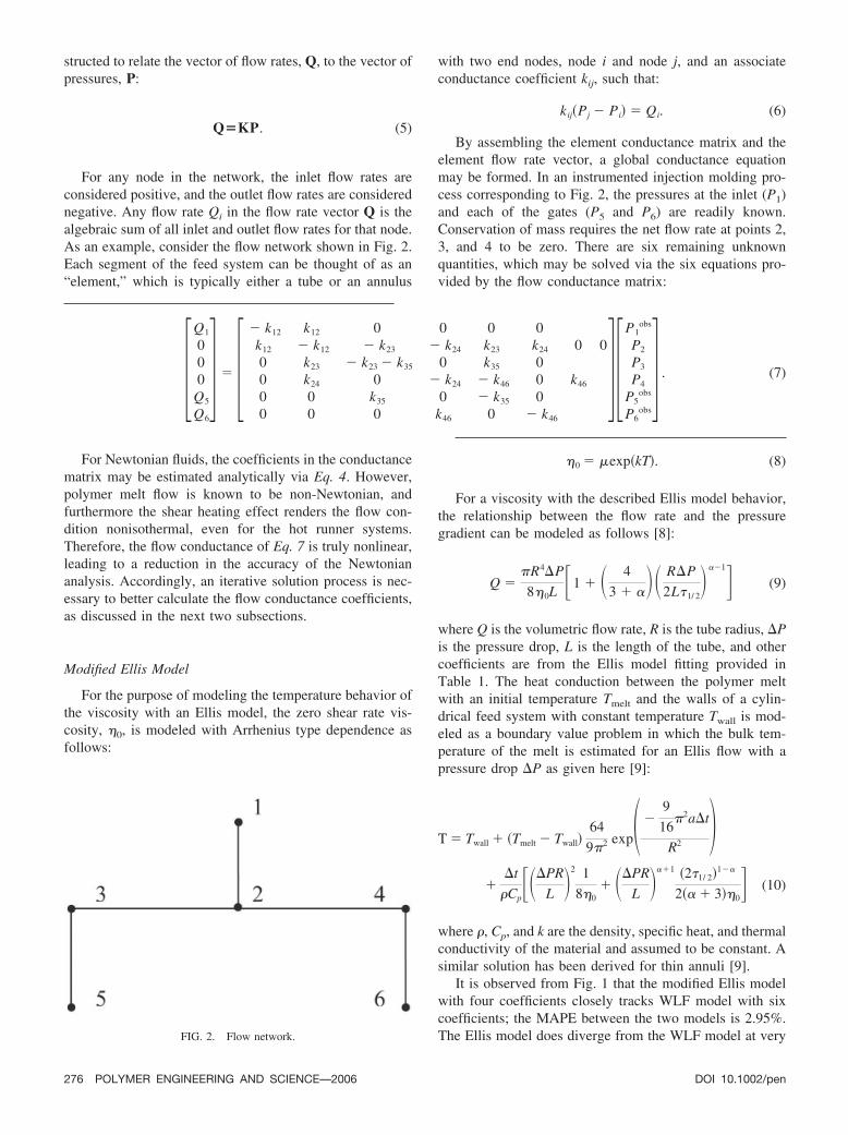
For any node in the network, the inlet flow rates areconsidered positive, and the outlet flow rates are considerednegative. Any flow rate Qi in the flow rate vector Q is thealgebraic sum of all inlet and outlet flow rates for that node.As an example, consider the flow network shown in Fig. 2.Each segment of the feed system can be thought of as an“element,” which is typically either a tube or an annulus

with two end nodes, node i and node j, and an associateconductance coefficient kij, such that:

kij�Pj Pi� � Qi. (6)

By assembling the element conductance matrix and theelement flow rate vector, a global conductance equationmay be formed. In an instrumented injection molding pro-cess corresponding to Fig. 2, the pressures at the inlet (P1)and each of the gates (P5 and P6) are readily known.Conservation of mass requires the net flow rate at points 2,3, and 4 to be zero. There are six remaining unknownquantities, which may be solved via the six equations pro-vided by the flow conductance matrix:

�Q1

000

Q5

Q6

� � � k12 k12 0 0 0 0k12 k12 k23 k24 k23 k24 0 00 k23 k23 k35 0 k35 00 k24 0 k24 k46 0 k46

0 0 k35 0 k35 00 0 0 k46 0 k46

��P1

obs

P2

P3

P4

P5obs

P6obs

� . (7)

For Newtonian fluids, the coefficients in the conductancematrix may be estimated analytically via Eq. 4. However,polymer melt flow is known to be non-Newtonian, andfurthermore the shear heating effect renders the flow con-dition nonisothermal, even for the hot runner systems.Therefore, the flow conductance of Eq. 7 is truly nonlinear,leading to a reduction in the accuracy of the Newtoniananalysis. Accordingly, an iterative solution process is nec-essary to better calculate the flow conductance coefficients,as discussed in the next two subsections.

Modified Ellis Model

For the purpose of modeling the temperature behavior ofthe viscosity with an Ellis model, the zero shear rate vis-cosity, �0, is modeled with Arrhenius type dependence asfollows:

�0 � �exp�kT�. (8)

For a viscosity with the described Ellis model behavior,the relationship between the flow rate and the pressuregradient can be modeled as follows [8]:

Q ��R4�P

8�0L�1 � � 4

3 � �� R�P

2L�1/ 2��1� (9)

where Q is the volumetric flow rate, R is the tube radius, �Pis the pressure drop, L is the length of the tube, and othercoefficients are from the Ellis model fitting provided inTable 1. The heat conduction between the polymer meltwith an initial temperature Tmelt and the walls of a cylin-drical feed system with constant temperature Twall is mod-eled as a boundary value problem in which the bulk tem-perature of the melt is estimated for an Ellis flow with apressure drop �P as given here [9]:

T � Twall � �Tmelt Twall�64

9�2 exp� 9

16�2a�t

R2 ��

�t

Cp��PR

L �2 1

8�0� ��PR

L ��1 �2�1/ 2�1��

2�� 3��0� (10)

where , Cp, and k are the density, specific heat, and thermalconductivity of the material and assumed to be constant. Asimilar solution has been derived for thin annuli [9].

It is observed from Fig. 1 that the modified Ellis modelwith four coefficients closely tracks WLF model with sixcoefficients; the MAPE between the two models is 2.95%.The Ellis model does diverge from the WLF model at veryFIG. 2. Flow network.

276 POLYMER ENGINEERING AND SCIENCE—2006 DOI 10.1002/pen

low shear rates (too abruptly transitioning to the Newtonianregime), at very high shear rates (underestimating the shearthinning effect of the polymer melt), and for very broadtemperature ranges (across which the Arrhenius temperaturedependence and constant �1/2 can induce significant errors).For this processing regime (spanning 20°C and 10,000sec�1), however, the modified Ellis model is a close ap-proximation to the rheological models used in sophisticatednumerical simulations and should provide very fast andreasonably accurate predictions. Even so, the assumption ofconstant thermal properties and bulk temperature across thethickness direction should result in less accurate results thanthose of numerical simulation, which is next described.

Numerical Simulation

The continuity equation, momentum equation, andenergy equation for nonisothermal polymer viscous flowin cylindrical coordinates are given by the followingequation:

�

�t�

�

� z(u) � 0 (11)

1

r

�

�r�r��u

�r� ��p

� z(12)

Cp��T

�t� u

�T

� z� �1

r

�

�r�rk�T

�r� � ��2 (13)

where u is the velocity in the flow direction, T is thetemperature, � is the viscosity predicted by the Cross-WLFmodel [6]. The boundary conditions for flow in tubes are asfollows:

u � 0 T � Tw2 at r � R2 (14)

�u

�r�

�T

�r� 0 at r � 0 (15)

where R2 is the outer radius and Tw2 is the wall temperature.Integrating Eq. 12 twice and applying the boundary

conditions of Eqs. 14 and 15 results in:

u � R2

�p

� z

r

2�dr. (16)

A similar solution can be derived for flow in thin annuli.The volumetric flow rate is given by

Q � 2�R1

R2

urdr � 2�� p

� z� S (17)

where for tubes,

S � 0

R2

� R2rdr

2� �rdr. (18)

The numerical solution proceeds as follows. At each timestep, the temperature field is calculated by the finite differ-ence method from the energy equation, Eq. 13. Then, theviscosity is calculated with the temperature field and theshear rate information from the previous time step. Theglobal conductance matrix K is then assembled. The knownpressures and flow rates can be given in arbitrary combina-tions of Pi and Qi, as long as the number of unknowns isequal to the number of nodes. With the estimated coeffi-cients, the unknown pressure variables are calculated fromthe flow conductance equation, Eq. 7. When all pressuresare known, the coefficients of the flow conductance matrixis updated by

kij � 2�S/L. (19)

With the new coefficients, the simulation recalculates thepressure and flow rate unknowns. This process proceedsuntil the change of the pressure unknowns is negligible,typically less than 0.01% of the previously calculated val-ues.

VALIDATION

Experimental Design

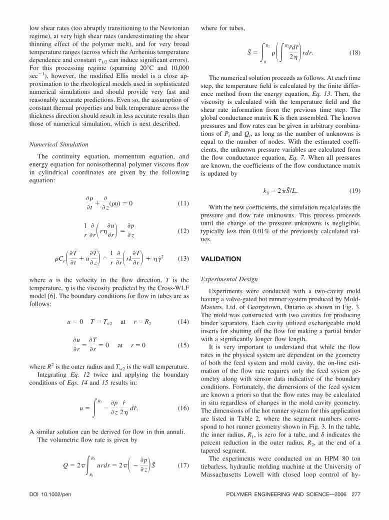
Experiments were conducted with a two-cavity moldhaving a valve-gated hot runner system produced by Mold-Masters, Ltd. of Georgetown, Ontario as shown in Fig. 3.The mold was constructed with two cavities for producingbinder separators. Each cavity utilized exchangeable moldinserts for shutting off the flow for making a partial binderwith a significantly longer flow length.

It is very important to understand that while the flowrates in the physical system are dependent on the geometryof both the feed system and mold cavity, the on-line esti-mation of the flow rate requires only the feed system ge-ometry along with sensor data indicative of the boundaryconditions. Fortunately, the dimensions of the feed systemare known a priori so that the flow rates may be calculatedin situ regardless of changes in the mold cavity geometry.The dimensions of the hot runner system for this applicationare listed in Table 2, where the segment numbers corre-spond to hot runner geometry shown in Fig. 3. In the table,the inner radius, R1, is zero for a tube, and � indicates thepercent reduction in the outer radius, R2, at the end of atapered segment.

The experiments were conducted on an HPM 80 tontiebarless, hydraulic molding machine at the University ofMassachusetts Lowell with closed loop control of hy-


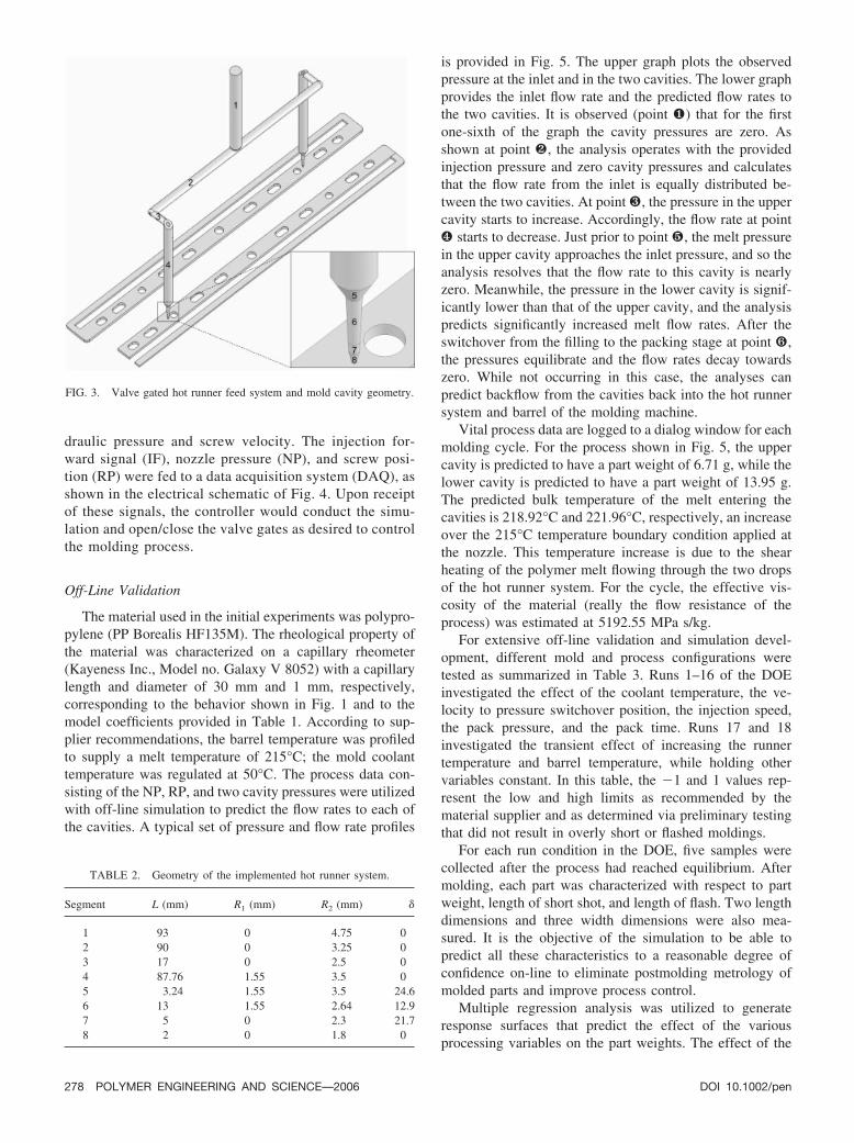
draulic pressure and screw velocity. The injection for-ward signal (IF), nozzle pressure (NP), and screw posi-tion (RP) were fed to a data acquisition system (DAQ), asshown in the electrical schematic of Fig. 4. Upon receiptof these signals, the controller would conduct the simu-lation and open/close the valve gates as desired to controlthe molding process.

Off-Line Validation

The material used in the initial experiments was polypro-pylene (PP Borealis HF135M). The rheological property ofthe material was characterized on a capillary rheometer(Kayeness Inc., Model no. Galaxy V 8052) with a capillarylength and diameter of 30 mm and 1 mm, respectively,corresponding to the behavior shown in Fig. 1 and to themodel coefficients provided in Table 1. According to sup-plier recommendations, the barrel temperature was profiledto supply a melt temperature of 215°C; the mold coolanttemperature was regulated at 50°C. The process data con-sisting of the NP, RP, and two cavity pressures were utilizedwith off-line simulation to predict the flow rates to each ofthe cavities. A typical set of pressure and flow rate profiles

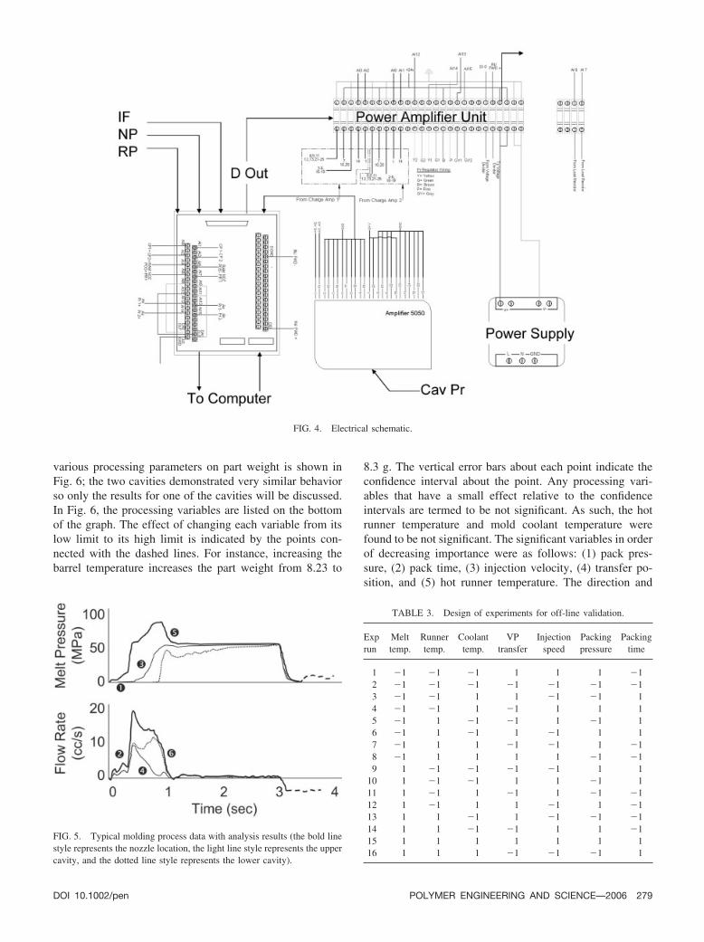
is provided in Fig. 5. The upper graph plots the observedpressure at the inlet and in the two cavities. The lower graphprovides the inlet flow rate and the predicted flow rates tothe two cavities. It is observed (point ) that for the firstone-sixth of the graph the cavity pressures are zero. Asshown at point , the analysis operates with the providedinjection pressure and zero cavity pressures and calculatesthat the flow rate from the inlet is equally distributed be-tween the two cavities. At point , the pressure in the uppercavity starts to increase. Accordingly, the flow rate at point

starts to decrease. Just prior to point , the melt pressurein the upper cavity approaches the inlet pressure, and so theanalysis resolves that the flow rate to this cavity is nearlyzero. Meanwhile, the pressure in the lower cavity is signif-icantly lower than that of the upper cavity, and the analysispredicts significantly increased melt flow rates. After theswitchover from the filling to the packing stage at point ,the pressures equilibrate and the flow rates decay towardszero. While not occurring in this case, the analyses canpredict backflow from the cavities back into the hot runnersystem and barrel of the molding machine.

Vital process data are logged to a dialog window for eachmolding cycle. For the process shown in Fig. 5, the uppercavity is predicted to have a part weight of 6.71 g, while thelower cavity is predicted to have a part weight of 13.95 g.The predicted bulk temperature of the melt entering thecavities is 218.92°C and 221.96°C, respectively, an increaseover the 215°C temperature boundary condition applied atthe nozzle. This temperature increase is due to the shearheating of the polymer melt flowing through the two dropsof the hot runner system. For the cycle, the effective vis-cosity of the material (really the flow resistance of theprocess) was estimated at 5192.55 MPa s/kg.

For extensive off-line validation and simulation devel-opment, different mold and process configurations weretested as summarized in Table 3. Runs 1–16 of the DOEinvestigated the effect of the coolant temperature, the ve-locity to pressure switchover position, the injection speed,the pack pressure, and the pack time. Runs 17 and 18investigated the transient effect of increasing the runnertemperature and barrel temperature, while holding othervariables constant. In this table, the �1 and 1 values rep-resent the low and high limits as recommended by thematerial supplier and as determined via preliminary testingthat did not result in overly short or flashed moldings.

For each run condition in the DOE, five samples werecollected after the process had reached equilibrium. Aftermolding, each part was characterized with respect to partweight, length of short shot, and length of flash. Two lengthdimensions and three width dimensions were also mea-sured. It is the objective of the simulation to be able topredict all these characteristics to a reasonable degree ofconfidence on-line to eliminate postmolding metrology ofmolded parts and improve process control.

Multiple regression analysis was utilized to generateresponse surfaces that predict the effect of the variousprocessing variables on the part weights. The effect of the

FIG. 3. Valve gated hot runner feed system and mold cavity geometry.

TABLE 2. Geometry of the implemented hot runner system.

Segment L (mm) R1 (mm) R2 (mm) �

1 93 0 4.75 02 90 0 3.25 03 17 0 2.5 04 87.76 1.55 3.5 05 3.24 1.55 3.5 24.66 13 1.55 2.64 12.97 5 0 2.3 21.78 2 0 1.8 0


various processing parameters on part weight is shown inFig. 6; the two cavities demonstrated very similar behaviorso only the results for one of the cavities will be discussed.In Fig. 6, the processing variables are listed on the bottomof the graph. The effect of changing each variable from itslow limit to its high limit is indicated by the points con-nected with the dashed lines. For instance, increasing thebarrel temperature increases the part weight from 8.23 to

8.3 g. The vertical error bars about each point indicate theconfidence interval about the point. Any processing vari-ables that have a small effect relative to the confidenceintervals are termed to be not significant. As such, the hotrunner temperature and mold coolant temperature werefound to be not significant. The significant variables in orderof decreasing importance were as follows: (1) pack pres-sure, (2) pack time, (3) injection velocity, (4) transfer po-sition, and (5) hot runner temperature. The direction and

FIG. 4. Electrical schematic.

FIG. 5. Typical molding process data with analysis results (the bold linestyle represents the nozzle location, the light line style represents the uppercavity, and the dotted line style represents the lower cavity).

TABLE 3. Design of experiments for off-line validation.

Exprun

Melttemp.

Runnertemp.

Coolanttemp.

VPtransfer

Injectionspeed

Packingpressure

Packingtime

1 �1 �1 �1 1 1 1 �12 �1 �1 �1 �1 �1 �1 �13 �1 �1 1 1 �1 �1 14 �1 �1 1 �1 1 1 15 �1 1 �1 �1 1 �1 16 �1 1 �1 1 �1 1 17 �1 1 1 �1 �1 1 �18 �1 1 1 1 1 �1 �19 1 �1 �1 �1 �1 1 1

10 1 �1 �1 1 1 �1 111 1 �1 1 �1 1 �1 �112 1 �1 1 1 �1 1 �113 1 1 �1 1 �1 �1 �114 1 1 �1 �1 1 1 �115 1 1 1 1 1 1 116 1 1 1 �1 �1 �1 1


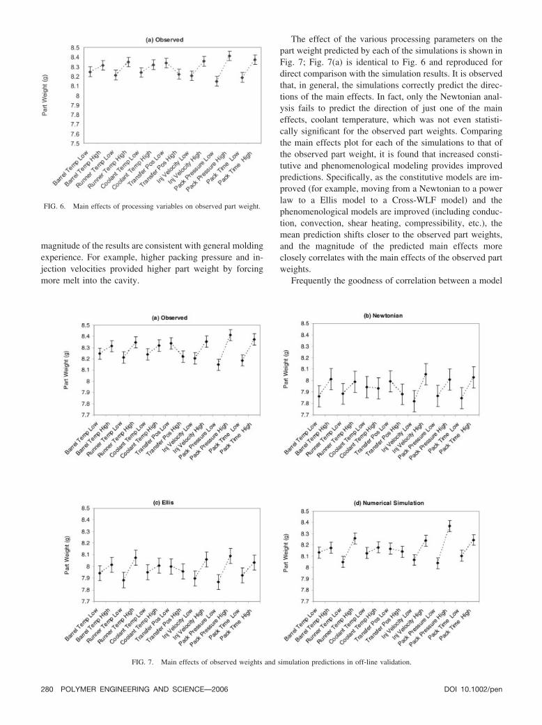
magnitude of the results are consistent with general moldingexperience. For example, higher packing pressure and in-jection velocities provided higher part weight by forcingmore melt into the cavity.

The effect of the various processing parameters on thepart weight predicted by each of the simulations is shown inFig. 7; Fig. 7(a) is identical to Fig. 6 and reproduced fordirect comparison with the simulation results. It is observedthat, in general, the simulations correctly predict the direc-tions of the main effects. In fact, only the Newtonian anal-ysis fails to predict the direction of just one of the maineffects, coolant temperature, which was not even statisti-cally significant for the observed part weights. Comparingthe main effects plot for each of the simulations to that ofthe observed part weight, it is found that increased consti-tutive and phenomenological modeling provides improvedpredictions. Specifically, as the constitutive models are im-proved (for example, moving from a Newtonian to a powerlaw to a Ellis model to a Cross-WLF model) and thephenomenological models are improved (including conduc-tion, convection, shear heating, compressibility, etc.), themean prediction shifts closer to the observed part weights,and the magnitude of the predicted main effects moreclosely correlates with the main effects of the observed partweights.

Frequently the goodness of correlation between a model

FIG. 6. Main effects of processing variables on observed part weight.

FIG. 7. Main effects of observed weights and simulation predictions in off-line validation.


and observed data is often expressed in terms of the coef-ficient of regression, R2:

R2 �SSR

SSR � SSE(20)

where SSE is the sum of square error between the modeloutput and the observed data and SSR is the sum of squaredresidual between the model output and the mean. The R2

value is a percentage of how well the model explains thevariability observed. Although a high R2 value means thatthe model closely matches the data, it is important to notethat high R2 values do not necessarily mean that the modelwill yield accurate predictions. Adding more terms to themodel will increase the value of R2, but not necessarilyincrease the accuracy of prediction. This is referred to as“over fitting” the data, and can be checked by calculatingother regression statistics such as the Radj

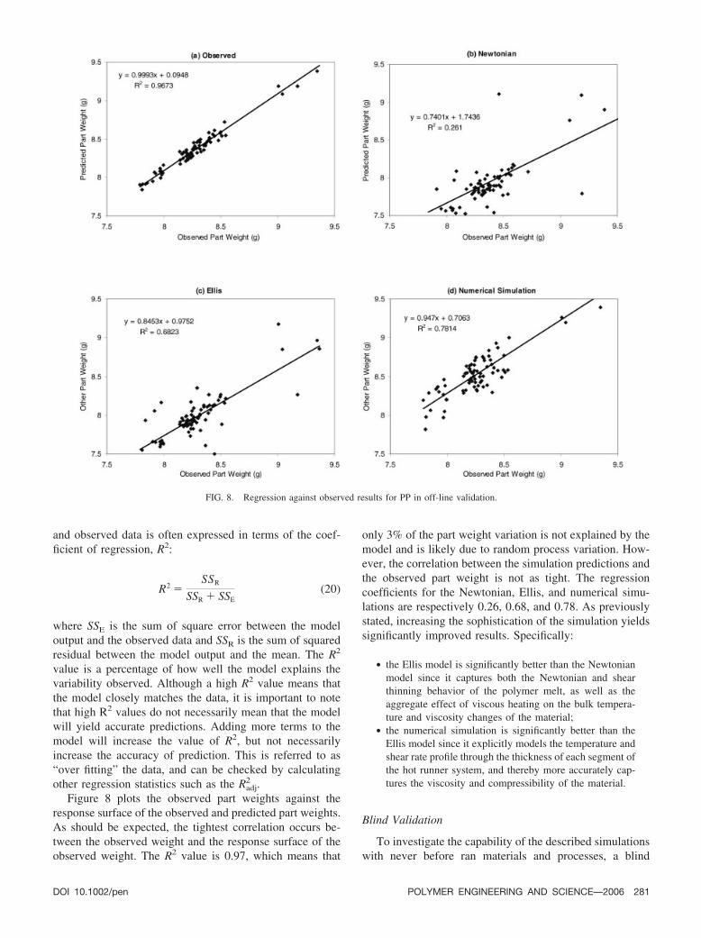
2 .Figure 8 plots the observed part weights against the

response surface of the observed and predicted part weights.As should be expected, the tightest correlation occurs be-tween the observed weight and the response surface of theobserved weight. The R2 value is 0.97, which means that

only 3% of the part weight variation is not explained by themodel and is likely due to random process variation. How-ever, the correlation between the simulation predictions andthe observed part weight is not as tight. The regressioncoefficients for the Newtonian, Ellis, and numerical simu-lations are respectively 0.26, 0.68, and 0.78. As previouslystated, increasing the sophistication of the simulation yieldssignificantly improved results. Specifically:

● the Ellis model is significantly better than the Newtonianmodel since it captures both the Newtonian and shearthinning behavior of the polymer melt, as well as theaggregate effect of viscous heating on the bulk tempera-ture and viscosity changes of the material;

● the numerical simulation is significantly better than theEllis model since it explicitly models the temperature andshear rate profile through the thickness of each segment ofthe hot runner system, and thereby more accurately cap-tures the viscosity and compressibility of the material.

Blind Validation

To investigate the capability of the described simulationswith never before ran materials and processes, a blind

FIG. 8. Regression against observed results for PP in off-line validation.


validation study was performed. In this program, four dif-ferent materials listed in Table 4 were investigated. Thematerials were chosen for their varying processing temper-atures, rheological properties, and thermal properties. Noneof the materials had been previously molded or otherwisetested, and the material properties were extracted directlyfrom a standard material database. Before molding, each ofthe material’s rheology was fit to the Newtonian and mod-ified Ellis models to minimize the variance across the ex-pected shear rate and temperature regime.

A half-factorial design of experiments (DOE [10]), pro-vided in Table 5, was conducted for each of the resins tocharacterize the effect of critical processing parameters onpart weight. This DOE was designed to capture four of thefive effects that were found significant in the off-line vali-dation, while avoiding undesirable transient effects associ-ated with changes in processing temperature. For each ma-terial, the molding process was operated at steady state for1 h before collecting samples. For each run in the DOE, aset of five parts was collected and analyzed with the threedescribed simulations. The simulation results were gener-ated before any metrology of the molded parts.

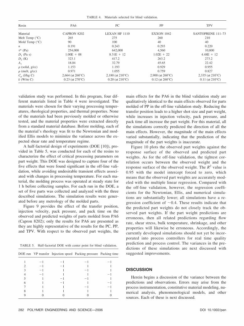
Figure 9 provides the effect of the transfer position,injection velocity, pack pressure, and pack time on theobserved and predicted weights of parts molded from PA6(Capron 8202); only the results for PA6 are presented asthey are highly representative of the results for the PC, PP,and TPV. With respect to the observed part weights, the

main effects for the PA6 in the blind validation study arequalitatively identical to the main effects observed for partsmolded of PP in the off-line validation study. Reducing thetransfer position leads to a higher shot size and part weight,while increases in injection velocity, pack pressure, andpack time all increase the part weight. For this material, allthe simulations correctly predicted the direction of all themain effects. However, the magnitude of the main effectsvaried substantially, indicating that the prediction of themagnitude of the part weights is inaccurate.

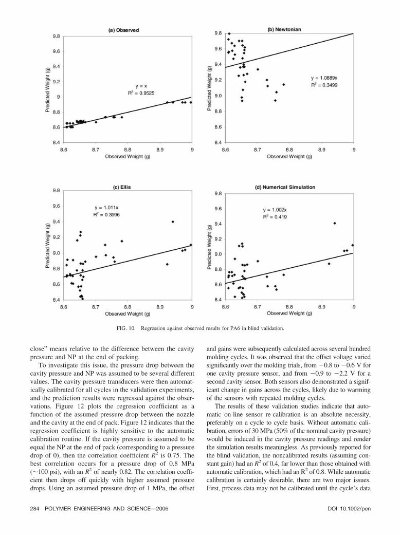
Figure 10 plots the observed part weights against theresponse surface of the observed and predicted partweights. As for the off-line validation, the tightest cor-relation occurs between the observed weight and theresponse surface of the observed weight. The R2 value is0.95 with the model intercept forced to zero, whichmeans that the observed part weights are accurately mod-eled with the multiple linear regression. Compared withthe off-line validation, however, the regression coeffi-cients for the Newtonian, Ellis, and numerical simula-tions are substantially lower; all simulations have a re-gression coefficient of �0.4. These results indicate thatthe predicted part weights do not closely track the ob-served part weights. If the part weight predictions areerroneous, then all related predictions regarding flowrate, shear stress, bulk temperature, shrinkage, and otherproperties will likewise be erroneous. Accordingly, thecurrently developed simulations should not yet be incor-porated into process controllers for real time qualityprediction and process control. The variances in the pre-dictions of these simulations are next discussed withsuggested improvements.

DISCUSSION

Herein begins a discussion of the variance between thepredictions and observations. Errors may arise from theprocess instrumentation, constitutive material modeling, nu-merical analysis, phenomenological models, and othersources. Each of these is next discussed.

TABLE 4. Materials selected for blind validation.

Resin PA6 PC PP TPV

Material CAPRON 8202 LEXAN HF 1110 EXXON 1042 SANTOPRENE 111–73Melt Temp (°C) 265 275 260 210Mold Temp (°C) 90 100 40 40n 0.191 0.243 0.293 0.220�* (Pa) 254,000 642,000 4,560 10,800D1 (Pa s) 1.00E � 08 8.31E � 12 1.02E � 22 4.48E � 12D2 (K) 323.1 417.2 263.2 273.2A1 18.04 32.79 45.65 22.42 (solid, g/cc) 1.153 1.193 0.929 0.955 (melt, g/cc) 0.971 1.055 0.759 0.827Cp (J/kg C) 2,664 (at 260°C) 2,180 (at 210°C) 2,900 (at 260°C) 2,335 (at 210°C)k (W/m C) 0.23 (at 270°C) 0.20 (at 210°C) 0.12 (at 260°C) 0.11 (at 210°C)

TABLE 5. Half-factorial DOE with center point for blind validation.

DOE run VP transfer Injection speed Packing pressure Packing time

1 �1 �1 �1 �12 �1 �1 1 13 �1 1 �1 14 �1 1 1 �15 1 �1 �1 16 1 �1 1 �17 1 1 �1 �18 1 1 1 19 0 0 0 0


Cavity Pressure Instrumentation and Calibration

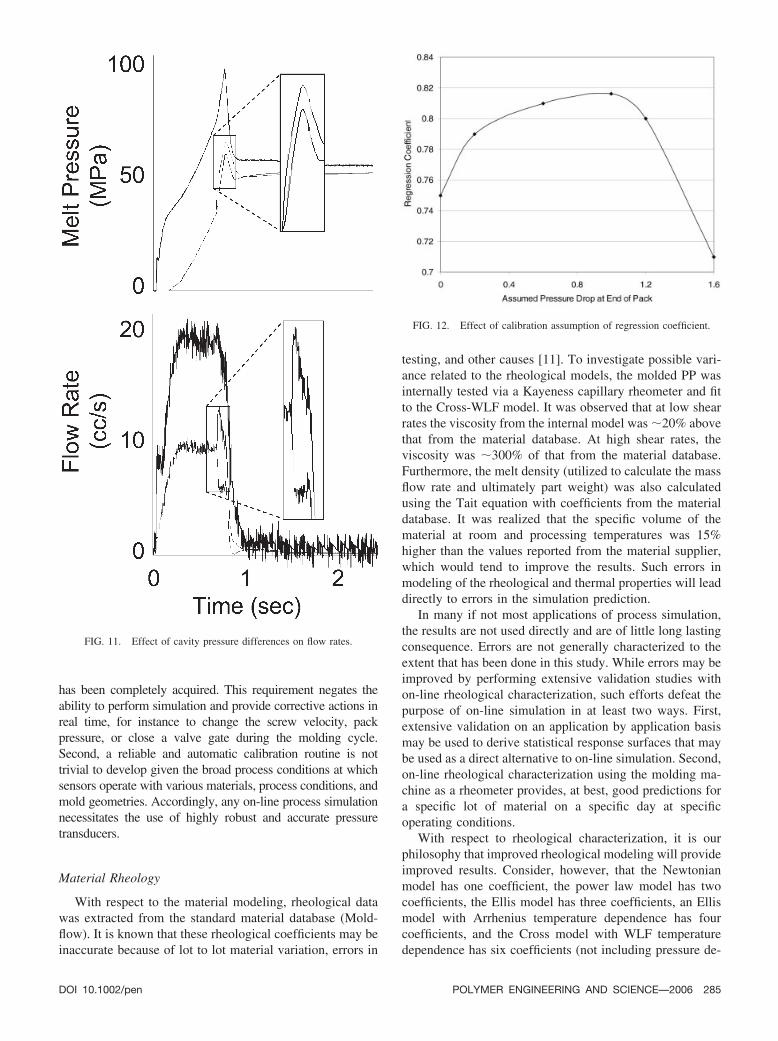
Real time process data are needed to perform on-lineprocess simulation. In particular, the simulation relies on thedifference between the cavity pressures and the NP tocalculate the flow rate of the melt going to each of thecavities. The key word in the previous sentence is differ-ence, which implies that very small differences in pressurescan lead to large differences in flow rate predictions. Thisrelationship is shown in Fig. 11. As shown in the figure, afew percent change in the cavity pressure can lead to a 40%change in the flow rates. This behavior may very well be areal occurrence that the simulation is correctly predicting. Ifthe pressure readings are erroneous by even one percent,however, very significant prediction errors will occur.

Upon investigation, both the off-line and the blind vali-dation studies showed very poor results when a constant setof signal conditioning values was used to relate outputvoltages from the pressure transducers to the melt pressuresin the cavities. To improve the simulation performance andto characterize the dependence of the simulation results onthe calibration of the cavity pressures, an automatic calibra-tion routine was developed to relate the output voltage, V,

from a transducer to the cavity pressure, P, according to theequation:

P � mV � b (21)

where b is the offset pressure when the voltage is zero andm is the pressure change per volt. For automatic calibration,some assumptions have to be made that relate the voltagesto the pressures. First, it is assumed that the nozzle andcavity pressures at the start of the cycle are zero. The offsetvoltage, b, can then be calculated by averaging a few of thereadings at the start of each cycle to reduce dependence ona single reading. Second, it is assumed that the cavitypressure at the end of the packing stage is “very close” tothe NP. This assumption may be valid since the flow ratesare very low at the end of the packing stage and the hotrunner system remains molten allowing nearly full trans-mission of the NP to the cavity. If this second assumptionholds, then the gain, m, for the cavity pressure transducersmay be calculated based on the NP at the end of packing foreach cycle. However, it is necessary to define what “very

FIG. 9. Main effects of observed weights and simulation predictions in blind validation.


close” means relative to the difference between the cavitypressure and NP at the end of packing.

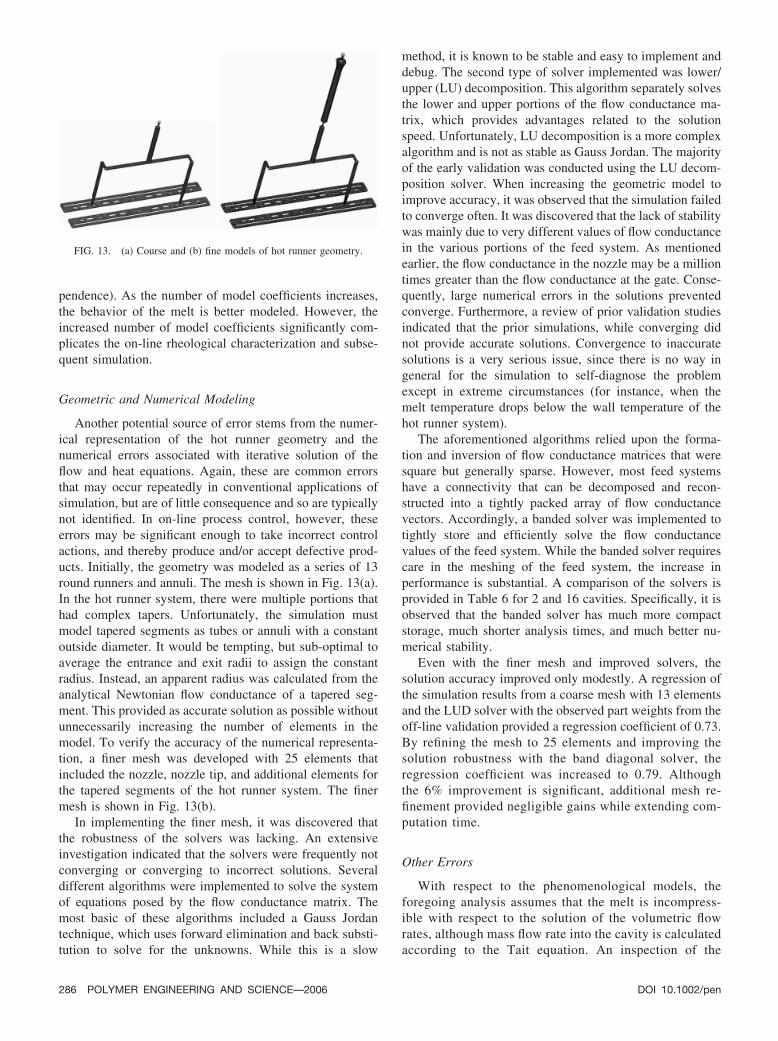
To investigate this issue, the pressure drop between thecavity pressure and NP was assumed to be several differentvalues. The cavity pressure transducers were then automat-ically calibrated for all cycles in the validation experiments,and the prediction results were regressed against the obser-vations. Figure 12 plots the regression coefficient as afunction of the assumed pressure drop between the nozzleand the cavity at the end of pack. Figure 12 indicates that theregression coefficient is highly sensitive to the automaticcalibration routine. If the cavity pressure is assumed to beequal the NP at the end of pack (corresponding to a pressuredrop of 0), then the correlation coefficient R2 is 0.75. Thebest correlation occurs for a pressure drop of 0.8 MPa(�100 psi), with an R2 of nearly 0.82. The correlation coeffi-cient then drops off quickly with higher assumed pressuredrops. Using an assumed pressure drop of 1 MPa, the offset

and gains were subsequently calculated across several hundredmolding cycles. It was observed that the offset voltage variedsignificantly over the molding trials, from �0.8 to �0.6 V forone cavity pressure sensor, and from �0.9 to �2.2 V for asecond cavity sensor. Both sensors also demonstrated a signif-icant change in gains across the cycles, likely due to warmingof the sensors with repeated molding cycles.

The results of these validation studies indicate that auto-matic on-line sensor re-calibration is an absolute necessity,preferably on a cycle to cycle basis. Without automatic cali-bration, errors of 30 MPa (50% of the nominal cavity pressure)would be induced in the cavity pressure readings and renderthe simulation results meaningless. As previously reported forthe blind validation, the noncalibrated results (assuming con-stant gain) had an R2 of 0.4, far lower than those obtained withautomatic calibration, which had an R2 of 0.8. While automaticcalibration is certainly desirable, there are two major issues.First, process data may not be calibrated until the cycle’s data

FIG. 10. Regression against observed results for PA6 in blind validation.


has been completely acquired. This requirement negates theability to perform simulation and provide corrective actions inreal time, for instance to change the screw velocity, packpressure, or close a valve gate during the molding cycle.Second, a reliable and automatic calibration routine is nottrivial to develop given the broad process conditions at whichsensors operate with various materials, process conditions, andmold geometries. Accordingly, any on-line process simulationnecessitates the use of highly robust and accurate pressuretransducers.

Material Rheology

With respect to the material modeling, rheological datawas extracted from the standard material database (Mold-flow). It is known that these rheological coefficients may beinaccurate because of lot to lot material variation, errors in

testing, and other causes [11]. To investigate possible vari-ance related to the rheological models, the molded PP wasinternally tested via a Kayeness capillary rheometer and fitto the Cross-WLF model. It was observed that at low shearrates the viscosity from the internal model was �20% abovethat from the material database. At high shear rates, theviscosity was �300% of that from the material database.Furthermore, the melt density (utilized to calculate the massflow rate and ultimately part weight) was also calculatedusing the Tait equation with coefficients from the materialdatabase. It was realized that the specific volume of thematerial at room and processing temperatures was 15%higher than the values reported from the material supplier,which would tend to improve the results. Such errors inmodeling of the rheological and thermal properties will leaddirectly to errors in the simulation prediction.

In many if not most applications of process simulation,the results are not used directly and are of little long lastingconsequence. Errors are not generally characterized to theextent that has been done in this study. While errors may beimproved by performing extensive validation studies withon-line rheological characterization, such efforts defeat thepurpose of on-line simulation in at least two ways. First,extensive validation on an application by application basismay be used to derive statistical response surfaces that maybe used as a direct alternative to on-line simulation. Second,on-line rheological characterization using the molding ma-chine as a rheometer provides, at best, good predictions fora specific lot of material on a specific day at specificoperating conditions.

With respect to rheological characterization, it is ourphilosophy that improved rheological modeling will provideimproved results. Consider, however, that the Newtonianmodel has one coefficient, the power law model has twocoefficients, the Ellis model has three coefficients, an Ellismodel with Arrhenius temperature dependence has fourcoefficients, and the Cross model with WLF temperaturedependence has six coefficients (not including pressure de-

FIG. 11. Effect of cavity pressure differences on flow rates.

FIG. 12. Effect of calibration assumption of regression coefficient.


pendence). As the number of model coefficients increases,the behavior of the melt is better modeled. However, theincreased number of model coefficients significantly com-plicates the on-line rheological characterization and subse-quent simulation.

Geometric and Numerical Modeling

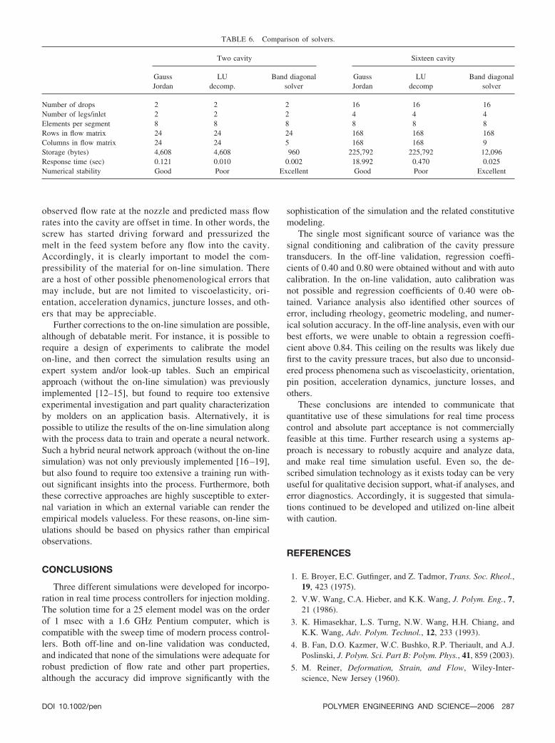
Another potential source of error stems from the numer-ical representation of the hot runner geometry and thenumerical errors associated with iterative solution of theflow and heat equations. Again, these are common errorsthat may occur repeatedly in conventional applications ofsimulation, but are of little consequence and so are typicallynot identified. In on-line process control, however, theseerrors may be significant enough to take incorrect controlactions, and thereby produce and/or accept defective prod-ucts. Initially, the geometry was modeled as a series of 13round runners and annuli. The mesh is shown in Fig. 13(a).In the hot runner system, there were multiple portions thathad complex tapers. Unfortunately, the simulation mustmodel tapered segments as tubes or annuli with a constantoutside diameter. It would be tempting, but sub-optimal toaverage the entrance and exit radii to assign the constantradius. Instead, an apparent radius was calculated from theanalytical Newtonian flow conductance of a tapered seg-ment. This provided as accurate solution as possible withoutunnecessarily increasing the number of elements in themodel. To verify the accuracy of the numerical representa-tion, a finer mesh was developed with 25 elements thatincluded the nozzle, nozzle tip, and additional elements forthe tapered segments of the hot runner system. The finermesh is shown in Fig. 13(b).

In implementing the finer mesh, it was discovered thatthe robustness of the solvers was lacking. An extensiveinvestigation indicated that the solvers were frequently notconverging or converging to incorrect solutions. Severaldifferent algorithms were implemented to solve the systemof equations posed by the flow conductance matrix. Themost basic of these algorithms included a Gauss Jordantechnique, which uses forward elimination and back substi-tution to solve for the unknowns. While this is a slow

method, it is known to be stable and easy to implement anddebug. The second type of solver implemented was lower/upper (LU) decomposition. This algorithm separately solvesthe lower and upper portions of the flow conductance ma-trix, which provides advantages related to the solutionspeed. Unfortunately, LU decomposition is a more complexalgorithm and is not as stable as Gauss Jordan. The majorityof the early validation was conducted using the LU decom-position solver. When increasing the geometric model toimprove accuracy, it was observed that the simulation failedto converge often. It was discovered that the lack of stabilitywas mainly due to very different values of flow conductancein the various portions of the feed system. As mentionedearlier, the flow conductance in the nozzle may be a milliontimes greater than the flow conductance at the gate. Conse-quently, large numerical errors in the solutions preventedconverge. Furthermore, a review of prior validation studiesindicated that the prior simulations, while converging didnot provide accurate solutions. Convergence to inaccuratesolutions is a very serious issue, since there is no way ingeneral for the simulation to self-diagnose the problemexcept in extreme circumstances (for instance, when themelt temperature drops below the wall temperature of thehot runner system).

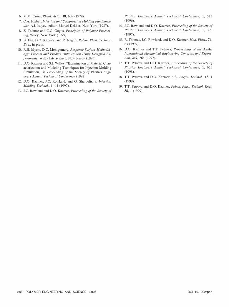
The aforementioned algorithms relied upon the forma-tion and inversion of flow conductance matrices that weresquare but generally sparse. However, most feed systemshave a connectivity that can be decomposed and recon-structed into a tightly packed array of flow conductancevectors. Accordingly, a banded solver was implemented totightly store and efficiently solve the flow conductancevalues of the feed system. While the banded solver requirescare in the meshing of the feed system, the increase inperformance is substantial. A comparison of the solvers isprovided in Table 6 for 2 and 16 cavities. Specifically, it isobserved that the banded solver has much more compactstorage, much shorter analysis times, and much better nu-merical stability.

Even with the finer mesh and improved solvers, thesolution accuracy improved only modestly. A regression ofthe simulation results from a coarse mesh with 13 elementsand the LUD solver with the observed part weights from theoff-line validation provided a regression coefficient of 0.73.By refining the mesh to 25 elements and improving thesolution robustness with the band diagonal solver, theregression coefficient was increased to 0.79. Althoughthe 6% improvement is significant, additional mesh re-finement provided negligible gains while extending com-putation time.

Other Errors

With respect to the phenomenological models, theforegoing analysis assumes that the melt is incompress-ible with respect to the solution of the volumetric flowrates, although mass flow rate into the cavity is calculatedaccording to the Tait equation. An inspection of the

FIG. 13. (a) Course and (b) fine models of hot runner geometry.


observed flow rate at the nozzle and predicted mass flowrates into the cavity are offset in time. In other words, thescrew has started driving forward and pressurized themelt in the feed system before any flow into the cavity.Accordingly, it is clearly important to model the com-pressibility of the material for on-line simulation. Thereare a host of other possible phenomenological errors thatmay include, but are not limited to viscoelasticity, ori-entation, acceleration dynamics, juncture losses, and oth-ers that may be appreciable.

Further corrections to the on-line simulation are possible,although of debatable merit. For instance, it is possible torequire a design of experiments to calibrate the modelon-line, and then correct the simulation results using anexpert system and/or look-up tables. Such an empiricalapproach (without the on-line simulation) was previouslyimplemented [12–15], but found to require too extensiveexperimental investigation and part quality characterizationby molders on an application basis. Alternatively, it ispossible to utilize the results of the on-line simulation alongwith the process data to train and operate a neural network.Such a hybrid neural network approach (without the on-linesimulation) was not only previously implemented [16–19],but also found to require too extensive a training run with-out significant insights into the process. Furthermore, boththese corrective approaches are highly susceptible to exter-nal variation in which an external variable can render theempirical models valueless. For these reasons, on-line sim-ulations should be based on physics rather than empiricalobservations.

CONCLUSIONS

Three different simulations were developed for incorpo-ration in real time process controllers for injection molding.The solution time for a 25 element model was on the orderof 1 msec with a 1.6 GHz Pentium computer, which iscompatible with the sweep time of modern process control-lers. Both off-line and on-line validation was conducted,and indicated that none of the simulations were adequate forrobust prediction of flow rate and other part properties,although the accuracy did improve significantly with the

sophistication of the simulation and the related constitutivemodeling.

The single most significant source of variance was thesignal conditioning and calibration of the cavity pressuretransducers. In the off-line validation, regression coeffi-cients of 0.40 and 0.80 were obtained without and with autocalibration. In the on-line validation, auto calibration wasnot possible and regression coefficients of 0.40 were ob-tained. Variance analysis also identified other sources oferror, including rheology, geometric modeling, and numer-ical solution accuracy. In the off-line analysis, even with ourbest efforts, we were unable to obtain a regression coeffi-cient above 0.84. This ceiling on the results was likely duefirst to the cavity pressure traces, but also due to unconsid-ered process phenomena such as viscoelasticity, orientation,pin position, acceleration dynamics, juncture losses, andothers.

These conclusions are intended to communicate thatquantitative use of these simulations for real time processcontrol and absolute part acceptance is not commerciallyfeasible at this time. Further research using a systems ap-proach is necessary to robustly acquire and analyze data,and make real time simulation useful. Even so, the de-scribed simulation technology as it exists today can be veryuseful for qualitative decision support, what-if analyses, anderror diagnostics. Accordingly, it is suggested that simula-tions continued to be developed and utilized on-line albeitwith caution.

REFERENCES

1. E. Broyer, E.C. Gutfinger, and Z. Tadmor, Trans. Soc. Rheol.,19, 423 (1975).

2. V.W. Wang, C.A. Hieber, and K.K. Wang, J. Polym. Eng., 7,21 (1986).

3. K. Himasekhar, L.S. Turng, N.W. Wang, H.H. Chiang, andK.K. Wang, Adv. Polym. Technol., 12, 233 (1993).

4. B. Fan, D.O. Kazmer, W.C. Bushko, R.P. Theriault, and A.J.Poslinski, J. Polym. Sci. Part B: Polym. Phys., 41, 859 (2003).

5. M. Reiner, Deformation, Strain, and Flow, Wiley-Inter-science, New Jersey (1960).

TABLE 6. Comparison of solvers.

Two cavity Sixteen cavity

GaussJordan

LUdecomp.

Band diagonalsolver

GaussJordan

LUdecomp

Band diagonalsolver

Number of drops 2 2 2 16 16 16Number of legs/inlet 2 2 2 4 4 4Elements per segment 8 8 8 8 8 8Rows in flow matrix 24 24 24 168 168 168Columns in flow matrix 24 24 5 168 168 9Storage (bytes) 4,608 4,608 960 225,792 225,792 12,096Response time (sec) 0.121 0.010 0.002 18.992 0.470 0.025Numerical stability Good Poor Excellent Good Poor Excellent


6. M.M. Cross, Rheol. Acta., 18, 609 (1979).

7. C.A. Hieber, Injection and Compression Molding Fundamen-tals, A.I. Isayev, editor, Marcel Dekker, New York (1987).

8. Z. Tadmor and C.G. Gogos, Principles of Polymer Process-ing, Wiley, New York (1979).

9. B. Fan, D.O. Kazmer, and R. Nageri, Polym. Plast. Technol.Eng., in press.

10. R.H. Myers, D.C. Montgomery, Response Surface Methodol-ogy: Process and Product Optimization Using Designed Ex-periments, Wiley Interscience, New Jersey (1995).

11. D.O. Kazmer and S.J. Willey, “Examination of Material Char-acterization and Modeling Techniques for Injection MoldingSimulation,” in Proceeding of the Society of Plastics Engi-neers Annual Technical Conference (1992).

12. D.O. Kazmer, J.C. Rowland, and G. Sherbelis, J. InjectionMolding Technol., 1, 44 (1997).

13. J.C. Rowland and D.O. Kazmer, Proceeding of the Society of

Plastics Engineers Annual Technical Conference, 1, 513(1996).

14. J.C. Rowland and D.O. Kazmer, Proceeding of the Society ofPlastics Engineers Annual Technical Conference, 1, 399(1997).

15. R. Thomas, J.C. Rowland, and D.O. Kazmer, Mod. Plast., 74,83 (1997).

16. D.O. Kazmer and T.T. Petrova, Proceedings of the ASMEInternational Mechanical Engineering Congress and Exposi-tion, 249, 264 (1997).

17. T.T. Petrova and D.O. Kazmer, Proceeding of the Society ofPlastics Engineers Annual Technical Conference, 1, 655(1998).

18. T.T. Petrova and D.O. Kazmer, Adv. Polym. Technol., 18, 1(1999).

19. T.T. Petrova and D.O. Kazmer, Polym. Plast. Technol. Eng.,38, 1 (1999).


Documents

Validation of three on-line flow simulations for injection molding