Validation of High-Fidelity CFD Simulations for Rocket Injector Design … · 2013-04-10 · Validation of High-Fidelity CFD Simulations for Rocket Injector Design P. Kevin Tucker1

Validation of High-Fidelity CFD Simulations for Rocket Injector Design

P. Kevin Tucker1 NASA Marshall Space Fight Center, Huntsville, AL, 35812

Suresh Menon2

Georgia Institute of Technology, Atlanta, GA, 30332

Charles L. Merkle3

Purdue University, West Lafayette, IN, 47907

Joseph C. Oefelein4

Sandia National Laboratories, Livermore, CA, 94551

and

Vigor Yang5

The Pennsylvania State University, University Park, PA, 16802

Computational fluid dynamics (CFD) has the potential to improve the historical rocket injector design process by evaluating the sensitivity of performance and injector-driven thermal environments to the details of the injector geometry and key operational parameters. Methodical verification and validation efforts on a range of coaxial injector elements have shown the current production CFD capability must be improved in order to quantitatively impact the injector design process. This paper documents the status of a focused effort to compare and understand the predictive capabilities and computational requirements of a range of CFD methodologies on a set of single element injector model problems. The steady Reynolds-Average Navier-Stokes (RANS), unsteady Reynolds-Average Navier-Stokes (URANS) and three different approaches using the Large Eddy Simulation (LES) technique were used to simulate the initial model problem, a single element coaxial injector using gaseous oxygen and gaseous hydrogen propellants. While one high-fidelity LES result matches the experimental combustion chamber wall heat flux very well, there is no monotonic convergence to the data with increasing computational tool fidelity. Systematic evaluation of key flow field regions such as the flame zone, the head end recirculation zone and the downstream near wall zone has shed significant, though as of yet incomplete, light on the complex, underlying causes for the performance level of each technique.

1 Aerospace Engineer and Combustion CFD Team Leader, MS ER42, NASA MSFC, AL 35812, Senior Member,

AIAA. 2 Professor and Director, Computational Combustion Laboratory, School of Aerospace Engineering, 270 Ferst Dr.,

Atlanta, GA 30332, Associate Fellow, AIAA. 3 Reilly Professor of Engineering, School of Mechanical Engineering, 585 Purdue Mall, West Lafayette, IN 47907,

Fellow, AIAA. 4 Principal Member of Technical Staff, Combustion Research Facility, 7011 East Avenue, MS9051, Livermore, CA

94550, Associate Fellow, AIAA. 5 J. L. and G. H. McCain Endowed Chair, Mechanical Engineering, 104 Research Building East, University Park,

PA 16802, Fellow, AIAA.

American Institute of Aeronautics and Astronautics

1

https://ntrs.nasa.gov/search.jsp?R=20080048109 2020-03-23T04:41:54+00:00Z

I. Introduction This paper documents the status of the first phase of an in-depth effort to evaluate CFD methodologies for

simulating rocket engine injectors. The overall effort, more fully documented contextually in Reference 1, consists of evaluating a hierarchy of methodologies using experimental data from three coaxial injector elements with hydrogen and oxygen propellants operating at supercritical conditions. There are two shear coaxial elements; Element 1 using gaseous oxygen and gaseous hydrogen with Element 2 using liquid oxygen and gaseous hydrogen. Element 3 is a swirl coaxial element using liquid oxygen and gaseous hydrogen propellants. This paper deals with the results from Element 1. It is the simplest of the group in terms of geometry, thermodynamics and physical processes.

The CFD methodologies evaluated range from RANS to LES. The current state of the practice in most injector design environments is axisymmetric RANS simulations of a single element due largely to the short turn around time imposed by the design cycle. This simulation fidelity has been shown to yield useful results for the shear coaxial element with gaseous propellants. 2 This is Element 1 of the current study. However, previous effort have shown results degrade to the point of little use as the complexity increases from Element 1 to Element 3.3 The objective of this part of the overall effort is to begin to understand what level of simulation fidelity is required to simulate the injector flow field with the combination of sufficient accuracy and affordable computational cost to be useful in the production computing environment inherent in the injector design process.

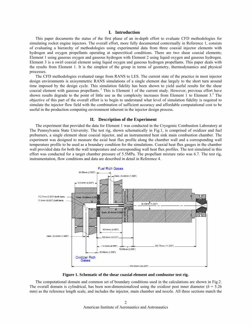
II. Description of the Experiment The experiment that provided the data for Element 1 was conducted in the Cryogenic Combustion Laboratory at

The Pennsylvania State University. The test rig, shown schematically in Fig.1, is comprised of oxidizer and fuel preburners, a single element shear coaxial injector, and an instrumented heat sink main combustion chamber. The experiment was designed to measure the axial heat flux profile along the chamber wall and a corresponding wall temperature profile to be used as a boundary condition for the simulations. Coaxial heat flux gauges in the chamber wall provided data for both the wall temperature and corresponding wall heat flux profiles. The test simulated in this effort was conducted for a target chamber pressure of 5.5MPa. The propellant mixture ratio was 6.7. The test rig, instrumentation, flow conditions and data are described in detail in Reference 4.

Figure 1. Schematic of the shear coaxial element and combustor test rig.

The computational domain and common set of boundary conditions used in the calculations are shown in Fig.2. The overall domain is cylindrical, has been non-dimensionalized using the oxidizer post inner diameter (δ = 5.26 mm) as the reference length scale, and includes the injector, main chamber and nozzle. All three sections match the


2

geometric profiles of the actual experimental apparatus. The injector section is 152 mm long, which provides appropriate entry lengths required for development of the turbulent boundary layers in the fuel and oxidizer streams. The total length of the combustion chamber and nozzle is 337 mm (286 and 51.0 mm, respectively). The inlet diameter of the central oxidizer jet is 7.92 mm. The exit diameter is 5.26 mm, and the oxidizer post is recessed 0.430 mm behind the chamber face. The inner and outer diameters at the inlet of the annular fuel jet are 12.7 and 25.4 mm, respectively. The corresponding exit diameters are 6.30 and 7.49 mm, respectively. The diameters of the combustion chamber, nozzle throat, and nozzle exit are 38.1, 8.17, and 12.0 mm, respectively. The composition, key reference properties, and flow characteristics of the oxidizer and fuel streams are listed in Table 1. The oxidizer stream

Figure 2. Computational domain and boundary conditions.

Table 1: Stream composition, reference properties, and flow characteristics of the oxidizer and fuel streams.

Oxidizer Stream Fuel Stream

Stream Composition:

Composition by Mass 0.945 (O2) / 0.0550 (H2O) 0.402 (H2) / 0.598 (H2O)

Composition by Volume 0.906 (O2) / 0.0940 (H2O) 0.857 (H2) / 0.143 (H2O)

Total Mass Flow Rate, kg/s 9.04 x 10-2 3.31 x 10-2

Reference Properties:

Pressure, MPa 5.2

Temperature, K 711 800

Density, kg/m3 26.8 3.33

Specific Heat (Cp), J/kg·K 1110

Ratio of Specific Heats 1.34 1.38

Dynamic Viscosity, Pa·s 3.62 x 10-5 1.81 x 10-5

Thermal Conductivity, W/m·K 0.0602 0.260

Kinematic Viscosity, m2/s 1.35 x 10-6 5.44 x 10-6

Thermal Diffusivity, m2/s 2.03 x 10-6 10.8 x 10-6

Sound Speed, m/s 513 1470

Flow Characteristics:

Bulk Velocity, m/s 68.0 (inlet) / 154 (exit) 25.9 (inlet) / 764 (exit)

Friction Velocity, m/s 2.77 (inlet) / 6.07 (exit) 1.31 (inlet) / 35.5 (exit)

Reynolds Number† 401,000(inlet) / 604,000 (exit) 60,000 (inlet) / 169,000 (exit)

Reynolds Number‡ 8170 (inlet) / 11900 (exit) 770 (inlet) / 1960 (exit) †Based on hydraulic diameter. ‡Based on friction velocity.


3

contains 0.906 moles of oxygen, 0.0940 moles of water, and is injected at a temperature of 711 K. The fuel stream contains 0.857 moles of hydrogen, 0.143 moles of water, and is injected at 800 K. Calculations were performed by applying constant flow rates of 0.0904 kg/s (oxidizer) and 0.0331 kg/s (fuel) at respective inlets. Supersonic boundary conditions are applied at the nozzle exit. No-slip conditions are applied at all wall surfaces. All of the injector wall surfaces are assumed to be adiabatic. The face of the combustion chamber and oxidizer post tip are assumed to be fixed at 755 K. The axial temperature distribution along the radial wall of the combustion chamber is obtained using available experimental measurements. A least squares fit of these data is used to approximate this distribution, as shown in Fig.2. The nozzle temperature is assumed to be fixed at 510 K. This value is consistent with the curve-fit, which by design provides a value of 510 K at the end of the combustion chamber with a gradient of zero. The reference pressure for the current calculations was set at 5.2 MPa. At this pressure the bulk exit velocities of the injector are 154 m/s for the oxidizer stream and 764 m/s for the fuel stream. The corresponding Reynolds numbers based on the hydraulic diameter (i.e., δ for the oxidizer stream and do – di for the fuel stream) are 604,000 and 169,000 respectively.

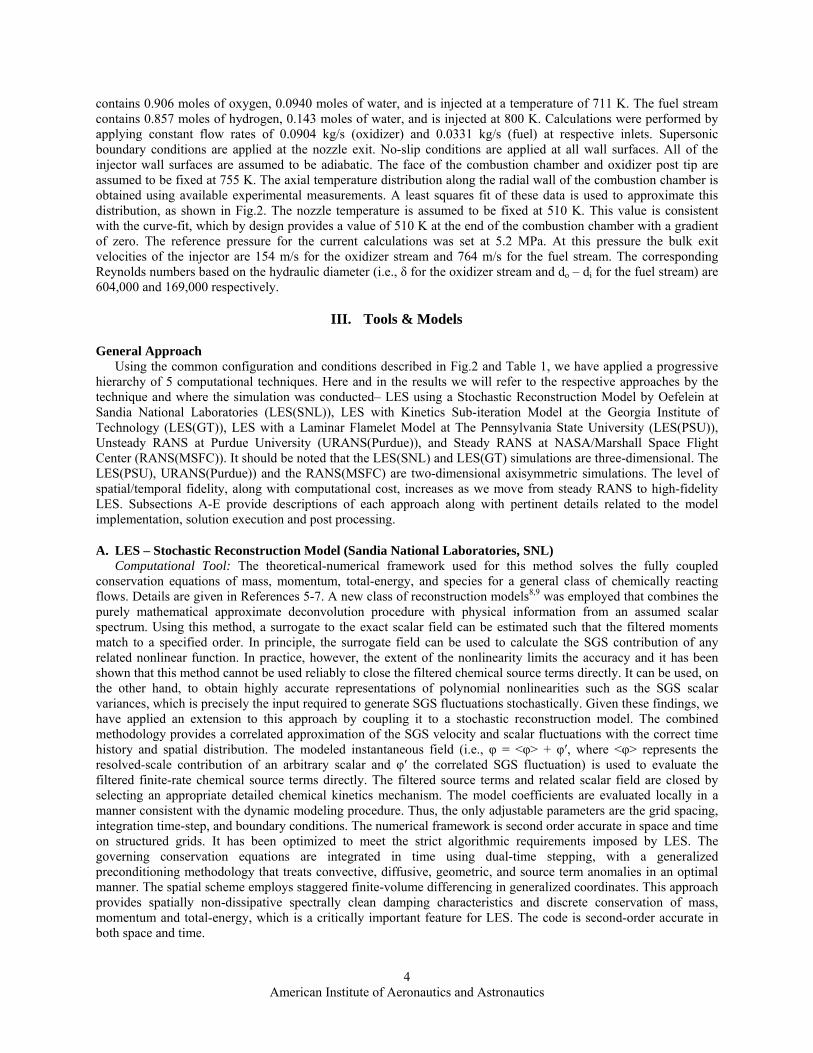
III. Tools & Models

General Approach Using the common configuration and conditions described in Fig.2 and Table 1, we have applied a progressive

hierarchy of 5 computational techniques. Here and in the results we will refer to the respective approaches by the technique and where the simulation was conducted– LES using a Stochastic Reconstruction Model by Oefelein at Sandia National Laboratories (LES(SNL)), LES with Kinetics Sub-iteration Model at the Georgia Institute of Technology (LES(GT)), LES with a Laminar Flamelet Model at The Pennsylvania State University (LES(PSU)), Unsteady RANS at Purdue University (URANS(Purdue)), and Steady RANS at NASA/Marshall Space Flight Center (RANS(MSFC)). It should be noted that the LES(SNL) and LES(GT) simulations are three-dimensional. The LES(PSU), URANS(Purdue)) and the RANS(MSFC) are two-dimensional axisymmetric simulations. The level of spatial/temporal fidelity, along with computational cost, increases as we move from steady RANS to high-fidelity LES. Subsections A-E provide descriptions of each approach along with pertinent details related to the model implementation, solution execution and post processing.

A. LES – Stochastic Reconstruction Model (Sandia National Laboratories, SNL) Computational Tool: The theoretical-numerical framework used for this method solves the fully coupled

conservation equations of mass, momentum, total-energy, and species for a general class of chemically reacting flows. Details are given in References 5-7. A new class of reconstruction models8,9 was employed that combines the purely mathematical approximate deconvolution procedure with physical information from an assumed scalar spectrum. Using this method, a surrogate to the exact scalar field can be estimated such that the filtered moments match to a specified order. In principle, the surrogate field can be used to calculate the SGS contribution of any related nonlinear function. In practice, however, the extent of the nonlinearity limits the accuracy and it has been shown that this method cannot be used reliably to close the filtered chemical source terms directly. It can be used, on the other hand, to obtain highly accurate representations of polynomial nonlinearities such as the SGS scalar variances, which is precisely the input required to generate SGS fluctuations stochastically. Given these findings, we have applied an extension to this approach by coupling it to a stochastic reconstruction model. The combined methodology provides a correlated approximation of the SGS velocity and scalar fluctuations with the correct time history and spatial distribution. The modeled instantaneous field (i.e., φ = <φ> + φ′, where <φ> represents the resolved-scale contribution of an arbitrary scalar and φ′ the correlated SGS fluctuation) is used to evaluate the filtered finite-rate chemical source terms directly. The filtered source terms and related scalar field are closed by selecting an appropriate detailed chemical kinetics mechanism. The model coefficients are evaluated locally in a manner consistent with the dynamic modeling procedure. Thus, the only adjustable parameters are the grid spacing, integration time-step, and boundary conditions. The numerical framework is second order accurate in space and time on structured grids. It has been optimized to meet the strict algorithmic requirements imposed by LES. The governing conservation equations are integrated in time using dual-time stepping, with a generalized preconditioning methodology that treats convective, diffusive, geometric, and source term anomalies in an optimal manner. The spatial scheme employs staggered finite-volume differencing in generalized coordinates. This approach provides spatially non-dissipative spectrally clean damping characteristics and discrete conservation of mass, momentum and total-energy, which is a critically important feature for LES. The code is second-order accurate in both space and time.


4

Model Implementation: Finite-rate chemical kinetics are modeled using the hydrogen-oxygen mechanism developed and optimized by Ó Conaire et al.10 A structured grid consisting of 255x106 cells was used to model the full three-dimensional computational domain with 31% of the cells in the injector and the remaining 69% in the chamber and nozzle. Even with such a large grid, some compromises were made with respect to strict resolution requirements because of the extremely high-Reynolds numbers associated with the case. Accordingly, the grid was optimized by maximizing the relative spacing in key sections while insuring that the near-wall boundary layer dynamics and peaks in the Reynolds-stress tensor are resolved to an acceptable level. The chamber grid was comprised of 1536 cells axially, 368 cells radially and 256 cells azimuthally. The injector post tip was modeled using 96 cells radially. The propellant inlet flow boundary was modeled using characteristic inflow with imposed mass flux. The nozzle exit flow boundary was modeled using a supersonic outflow boundary condition. The chamber was initialized with the theoretical combustion products and temperature for the experimental mixture ratio and chamber pressure. The initial chamber velocity was set using the density of the theoretical combustion products, while the nozzle velocity was initialized with a one-dimensional solution for converging-diverging nozzles. Simulation Execution & Post Processing: The solution was obtained using an integration time step of 0.068 μs over 720,000 time-steps to simulate six chamber flow-through times. This amounts to approximately 50 ms of injector operation. In this work, a flow through time of 8.3 ms was defined using the bulk mass flow in the chamber, theoretical combustion products and chamber diameter. Using this definition, the simulation ran for four flow-through times to reach a statistically steady solution, after which it was run for another two flow-through times to obtain time-averaged data. The time-averaged solutions shown later are also spatially averaged over the 256 azimuthal planes. The entire simulation required approximately 2 million cumulative CPU hours using an average of 2000 processors.

B. LES – Kinetics with Sub-iteration Model (Georgia Institute of Technology, GT) Computational Tool: The simulation software LESLIE3D is a fully compressible, finite-volume solver

developed at Georgia Tech that is second-order accurate in space and time. It employs a hybrid approach that combines a predictor-corrector scheme in smooth flow regions and a 3rd-order MUSCL upwind-biased flux extrapolation scheme with a Harten-Lax-Leer (HLL) type limiter in regions of very high gradients and/or contact discontinuities. A monotonized central limiter is used to enforce the total variation diminishing condition. Switching between the two algorithms is dynamic and local.11 The SGS closure employs a transport model for the subgrid kinetic energy to determine the sub-grid eddy viscosity used to close the sub-grid stresses and energy flux, as well as to determine the sub-grid eddy diffusivity used to close the sub-grid scalar flux. The 21-step; 8-species mechanism of Ó Conaire et al.10 is employed for a thermally perfect gas. For this simulation, as a compromise between the cost and the accuracy of the numerical integration, a simple Euler time-integration with 20 sub-iterations was used instead of exactly solving the system of differential equations. This method was chosen because of the relative fast chemistry coupled with the relatively low levels of subgrid kinetic energy in the shear layer. Analysis of the reaction and mixing time scales showed that the current closure captures reaction kinetics within each LES cell at a time-step small enough to resolve the critical elementary reactions using the sub-iteration approach12. Effects of subgrid diffusion and turbulent stirring as in the LEM approach11,12 will be considered in the future.

Model Development: A structured body conforming grid is used to model the full 3D computational domain. The multi-block grid is cylindrical with dimensions of 611x87x65 with an inner “butterfly” Cartesian section of dimensions 611x17x17 to eliminate the centerline singularity. Overall, the total number of cells where computation is performed is 3.16x106 since some cells in the inlet portion of the domain were blanked out. The injector portion of the geometry was limited to a region 50.0 mm upstream of the injector face to reduce the over-all grid size. Approximately 10% of the cells were used to model the inlets upstream of the injector face and 8% are used in the nozzle, with the remaining 2.5x106 cells used to model the cylindrical part of the combustion chamber. Clustering is employed in the shear layer and in the post region, with very small stretching factors in the regions of interest. The oxidizer post tip is resolved with 11 points in the radial direction, which results in a 0.043 mm grid spacing. The radial grid distribution in the oxygen and hydrogen streams is approximately similar in resolution. The axial grid is clustered near the injector tip and then stretches slowly to the beginning of the nozzle, after which the grid is maintained uniform. The grid resolution near the injector post is able to capture a clear inertial range and therefore, shows adequate resolution for a LES. However, the grid is not densely clustered along the chamber wall where the heat transfer is calculated; this is considered a limitation of the current simulation.

The propellant inlet flow boundary is modeled using characteristic inflow with imposed mass flux. Injector inflow conditions are chosen based on a separate simulation of the full injector region and applied using characteristic inflow conditions. The nozzle exit flow boundary is modeled using a supersonic outflow boundary condition. The combustion chamber is initialized using a volumetric composition of 90% (H2O), 10% (OH), and a


5

temperature of 3000 K. The initial chamber pressure is set to 5.2 MPa, and the calculation is started with a reduced 2-step mechanism and run for approximately two flow-through times to flush out the initial transient. Afterwards, the full kinetics mechanism is employed.

Simulation Execution & Post Processing: The simulation is carried out using an integration time step of 0.010 μs for over four million iterations to simulate approximately five chamber flow-through times (8.3 ms each). Overall, an equivalent of over 500,000 single processor hours was required on an Intel Xeon PC cluster for the entire simulation, and a typical run employed 256 processors. The choice of the number of processors was limited by current resource availability. However, the code shows over 85% scalability up to 1024 processors. The initial two flow-through time transient was discarded and then the simulation data was time-averaged over three flow-through times. The time-averaged solutions shown later are also spatially averaged over the 64 azimuthal planes.

C. LES – Flamelet Model (The Pennsylvania State University, PSU) Computational Tool: The basis of this approach is the general theoretical-numerical framework described in

References 13-15. The formulation accommodates the full conservation laws for a multicomponent chemically reacting system. Full account is taken of real-fluid thermodynamics and transport over the entire temperature and pressure regimes of concern. Thermodynamic properties, such as internal energy, enthalpy, and constant-pressure specific heat, are obtained directly from fundamental thermodynamics theories.16 Transport properties are estimated using an extended corresponding-state theory. SGS turbulence-chemistry interactions are treated by means of a mixture-fraction based flamelet model. The approach assumes that chemical scales are shorter than the Kolmogorov scales of turbulent flows. Consequently, a turbulent flame can be envisioned as a synthesis of thin reaction zones embedded in an otherwise inert turbulent flow field and the inner structure of the flame can be handled separately from turbulent flow simulations. Instead of directly treating reactive scalars, the focus of the flamelet model is placed on the identification of the flame surface in the flow field, which can be obtained by solving the conservation equation of the mixture fraction in a coupled manner with the mass, momentum, and energy equations. Because the flame thickness is typically smaller than the grid size, the influence of the SGS mixture fraction variance on the flame behavior is modeled either by a presumed δ- or a β-shaped probability density function (PDF). Once the solution of the mixture fraction and its variance are acquired, the species mass fractions are evaluated using a pre-established flamelet library based on a series of numerical solutions of counterblow hydrogen/oxygen diffusion flames.17 The flame solutions were carried over a wide range of flow strain rates with a detailed reaction mechanism including 8 species (i.e., H2, O2, H, O, OH, HO2, H2O, and H2O2) and 19 reversible reactions. The numerical implementation is fourth-order accurate in space and second-order accurate in time. It incorporates general-fluid thermodynamics and transport theories into a preconditioning scheme along with a dual time-stepping integration algorithm.18,19 All the numerical properties, including the preconditioning matrix, Jacobian matrices, and eigenvalues, are derived directly from fundamental thermodynamics theories, rendering a self-consistent and robust algorithm. A multiblock domain decomposition technique, along with static load balancing, was employed to facilitate efficient parallel computations using MPI. The parallelization methodology is robust and the speedup is almost linear.

Model Implementation: The structured grid used for the two-dimensional axisymmetric simulation was 750x350 cells in the axial and radial directions, respectively. The 262,500 cell mesh was decomposed into 71 blocks for parallel execution. Forty cells were used to radially resolve the injector post tip. Special attention was paid to the grid resolution close to the chamber wall in order to facilitate an accurate prediction of the wall heat flux. The initial grid stretching ratio is 1.02. For both propellant inlets, the bulk axial velocities of oxygen and hydrogen streams are selected to match the mean mass flow rates. The temperatures of both streams were fixed and pressure was obtained through a one-dimensional approximation to the axial momentum equation. A supersonic outlet boundary was employed at the downstream boundary. The simulation was initialized using a RANS approximation to provide a reasonable initial condition for the LES calculation. The combustor was preconditioned with a mixture of oxygen (0.3 by mass), hydrogen (0.3), and water vapor (0.4). The chamber pressure was set at 5.2 MPa. The steady-state solution obtained from the RANS calculation was then interpolated and mapped onto the LES grid as the initial condition for the LES simulation.

Model Execution & Post Processing: The validity of the flamelet model under the present simulation conditions was confirmed through a careful comparison of the characteristic chemical and turbulent time scales over the entire flowfield.20 Specifically, the Kolmogorov time scale evaluated based on the LES simulation results was 1.2 x 10-6 s at the axial location 5 mm downstream of the injector faceplate. The characteristic chemical time scale of 5.48 x 10-7 s obtained from flame calculation was over two times smaller than this value.

Temporal integration was obtained through a dual-time step integration technique. The physical time step was 0.1 μs, and the maximum CFL number for the inner loop integration in pseudo-time was 0.7. Approximately five


6

flow-through times were simulated, requiring about 400,000 iterations to simulate 40 ms of combustor operation. The simulation required approximately 100,000 CPU hours on 71 2.2 GHz Pentium IV processors.

The initial transient of one flow-through time was discarded. The simulation data was time-averaged over the last four flow-through times. The integration time step was fixed, so all mean flow properties were evaluated by a simple arithmetic average using the number of time steps. Since the simulation is two-dimensional, no spatial averaging was required in the azimuthal direction.

D. Unsteady RANS (Purdue University, Purdue) Computational Tool: The General Equation and Mesh Solver (GEMS) code solves the Navier-Stokes, energy

and species continuity equations in coupled fashion. GEMS is an unstructured solver with parallel capability. The code is implicit and second order accurate in both space and time on structured grids. GEMS uses an upwind approximate Riemann solver in space and a dual time procedure. Thermodynamic and transport properties of all species are expressed as arbitrary functions of pressure and temperature with appropriate mixing relations used to obtain mixture properties. Enthalpies, viscosity and thermal conductivity for each species are taken from polynomial expressions. Species diffusivities are obtained from a Chapman-Enskog expression. Turbulence was incorporated by means of the Spalart-Allmaras model with integration to the wall. To control the levels of eddy viscosity in the free-stream, the dissipation term in the turbulence model was reduced in regions far from the walls. A 9 species, 17 reaction step chemical kinetics model was used to represent the combustion of hydrogen and oxygen. Additional details are given in References 21 and 22.

Model Implementation: A two-dimensional axisymmetric representation of the injector and combustor was discretized using a structured mesh consisting of approximately 250,000 cells. The grid was resolved to y+ = 1 at all walls with geometric stretching toward the free stream such that approximately 15 points were placed within y+ = 30. The injector post tip was resolved with 70 grid points. The upstream boundary conditions for both propellants were specified mass flow rate and specified stagnation enthalpy. A short divergent nozzle in conjunction with a back pressure boundary condition low enough to insure choking at the throat provided the downstream boundary condition.

The URANS simulation employed a unique initialization and flow initiation process. The first three-fourths of the fuel passage were filled with fuel at the appropriate temperature from the experiment. Likewise, the first three-fourths of the fuel passage were filled with oxidizer at the appropriate temperature. The remainder of the propellant inlet passages and the chamber were filled with a specially defined fluid (‘nitrogen’) that was distinct from any of the other eight species. The ‘nitrogen’ temperature was set to 1500K. All velocity components were set to zero throughout the domain. The initial pressure was set to 3.24 MPa, which corresponds to pressure generated in the chamber with 1500 K nitrogen passing through the choked throat at the same mass flow rate as the incoming propellants. Flow was initiated by breaking ‘diaphragms’ at the fuel and oxidizer inlets and the nozzle exit. Resulting compression waves in injector passages initiates propellant flows and starts the flow into chamber. The resulting expansion wave from exit plane rapidly chokes nozzle and allows chamber pressure to increase with time. Ignition occurs spontaneously when initial hydrogen and oxygen come into contact upon mixing. The heated inert fluid in the chamber provides sufficient pre-heat to initial portions of incoming fluid to allow ignition.

The initial ‘nitrogen’ in the chamber and inlet tubes served two purposes. First, since neither the incoming fuel nor oxygen contain nitrogen, the amount of residual nitrogen in the computational domain immediately indicates the degree to which the initial condition still impacts the predictions. Unambiguous results clearly require that the nitrogen concentration be reduced to a negligible magnitude at every point throughout the domain. The second function of the nitrogen was to prevent combustion between hydrogen and oxygen until mixing started, with the 1500K initial temperature being chosen to ensure spontaneous ignition as soon as fuel and oxidizer came together so that no amount of pre-mixing would be tolerated. This resulted in a very smooth and well controlled ignition process that avoided large acoustic oscillations caused by ignition of a finite mass of propellant. Model Execution and Post Processing: The solution was obtained using an integration time step of 0.1 μs over 550,000 time-steps to simulate almost seven chamber flow-through times. This amounts to approximately 55 ms of injector operation. The simulation ran on 30 processors consuming about 25,000 CPU hours. The time averaging processes commenced after 45 ms when all initial ‘nitrogen’ had been flushed out of the chamber. The averaging was done by summing results of individual time steps over 3 ms intervals.

E. Steady RANS (Marshall Space Flight Center, MSFC) Computational Tool: Loci-CHEM is a finite-volume flow solver for generalized grids developed at Mississippi

State University in part through NASA and NSF funded efforts. Loci-CHEM is second- order accurate in both space and time. It uses high resolution approximate Riemann solvers to solve turbulent flows with finite-rate chemistry.


7

Preconditioning23 is available for low Mach number applications. Details of the numerical formulation are given in the Loci-CHEM user guide.24 Loci-CHEM is comprised entirely of C and C++ code and is supported on all popular UNIX variants and compilers. Efficient parallel operation is facilitated by the Loci25 framework which exploits multi-threaded and MPI libraries. The Mentor Shear Stress Transport26 (SST) was used in the current effort. The model used for finite-rate hydrogen-oxygen chemistry was a 6 species 28 reaction scheme.27 Thermodynamic properties are obtained using a standard partition function formulation which calculates the specific heats, internal energies and entropies of each individual perfect gas species.

Model Implementation: The hybrid two-dimensional axisymmetric mesh was generated using GRIDGEN Version 15 from Pointwise Corporation.28 The hybrid mesh was generated by extruding connectors representing the axisymmetric solid surfaces normal to the solid surface into the computational domain with an initial spacing and stretch rate defined. The extrusion was terminated at the location where the extruded cells possessed an aspect ratio of approximately unity. This allowed a good quality transition from structured to unstructured cell types. The remainder of the computational domain was meshed using unstructured cells with a boundary decay factor of approximately 0.995. The hybrid mesh used for this simulation contained approximately 400,000 cells. The injector post tip was modeled using 43 cells radially. Solutions on numerous finer and coarser grid variations were obtained to confirm grid convergence.

The propellant inflow boundary conditions were fixed mass flow rate with the temperatures fixed at the experimental values. The nozzle exit boundary condition was a supersonic outflow. Inlet boundary values for turbulence quantities, k and omega, were specified as 5x10-6 m2/s2 and 500 1/s respectively. While these values are lower than those recommended,34 the turbulent field develops in the injector inlets and previous experience has shown that the injector inlet distances in this case allow no sensitivity of the chamber solution to the injector inlet turbulence quantities specification. The computational domain was initialized with quiescent steam at 780 K to start the steady state simulation. The steam provided a high enough initial temperature such that when the reactant streams reached the post-tip region and mixed self-ignition occurred.

Model Execution and Post Processing: The model was executed in local time stepping mode with a physical time step of 100 μs. This time step was dynamically reduced locally to not exceed a maximum CFL number of 10,000 or a change in temperature, pressure or density variables of more than 10 percent per time step. With these settings, the model ignited relatively smoothly and ignition did not cause any sustained reverse flow of propellants into either the fuel or oxidizer inlet tubes. The simulation required about 10,000 time steps to achieve steady state convergence. A typical calculation using 16 AMD Opteron 246 processors required approximately 1,600 CPU hours. As long as the number of cells per processor remains similar to that described above, the Loci-CHEM is nearly perfectly scalable.

Solution convergence was evaluated by a combination of residual drop, total mass flow convergence in terms of integrated mass at inlet verses integrated mass at outlet, species stored mass convergence integrated over the entire domain volume, and temperature and pressure iteration history at selected probe point locations throughout the flow-field. In addition the chamber wall heat flux was monitored until convergence was confirmed. Three orders of magnitude of residual drop were observed. Computational domain mass conservation was achieved to with 0.1 percent of the total mass flow. The species stored masses were also driven down to less than 0.1 percent of the total stored mass of that species. The probe point pressure and temperature variations are driven down to less than 0.1 percent of the steady state average.

No spatial or temporal averaging was required for this steady axisymmetric simulation.

IV. Results The five methodologies described in Section III represent a hierarchy in terms of fidelity and computational

expense, with the highest fidelity tools being the most expensive to use. Thus, we refer to these in the discussion below from high fidelity/expense to low fidelity/expense as LES(SNL), LES(GT), LES(PSU), URANS(Purdue) and RANS(MSFC). LES(SNL) and LES(GT) are the simulations by Oefelein and Menon and are both three-dimensional (3D) LES. LES(PSU) is the simulation by Yang and is a two-dimensional (2D) axisymmetric LES. Finally, the URANS(Purdue) and RANS(MSFC) are the simulations performed by Merkle and Tucker et al. and are 2D axisymmetric unsteady and steady RANS implementations, respectively. Recall that the objectives of the overall effort on the three coaxial elements are to determine the trades between simulation accuracy and expense represented by this hierarchy of methodologies and to determine how to use this information to provide results with sufficient accuracy but are computationally affordable in a design environment.


8

Figure 3. Heat flux predictions from respective calculations compared with

corresponding experimental data.

The heat flux predictions from each of the five simulations are plotted in Fig. 3 along with the experimental data. The experimental data is indicated with symbols and the simulation results are noted by lines. The experimental data shows that the heat flux rises very rapidly in the head end of the chamber as the propellants begin to react. The heat flux has an almost flat peak from 0.03 meters to 0.09 meters downstream of the injector face at a value of approximately 16 MW/m2. From the peak, the heat flux value gradually decreases with axial distance until the last measured value of just over 5 MW/m2 near the chamber exit. The heat flux rise rate and the peak heat flux value are important injector design considerations when considering thermal compatibility with the combustion chamber. Also, the heat flux rise rate can be used to make qualitative inferences about the rate of combustion and thus, element efficiency. To facilitate the discussion of results, the chamber is divided into two sections; a head-end section, 0 ≤ x ≤ 0.1 meters, where x is the axial distance and a downstream section from 0.1 meters to about 0.26 meters, which is the end of the constant area section of the chamber.

Some general observations can be made by looking at Fig. 3. First, there is clearly no monotonic convergence of the results to the data with respect to increasing model fidelity. This, in a sense, is not surprising since there are many complexities and details in both the modeling assumptions and implementation requirements in all five of the approaches. It does, however, significantly complicate the analysis of the results. Second, the two 3D time-averaged predictions are smoother than the other three results. This is due to additional averaging in the azimuthal direction (i.e., a much larger sample space was used to construct the average). Third, the LES(SNL) result provides by far the best match to the experimental data over the entire length of the chamber. This was expected since it was the highest fidelity simulation. Last, the other four calculations match the data fairly well over discrete portions of the chamber wall, but none as consistently as LES(SNL).

Looking at more detailed trends in Fig. 3, the RANS(MSFC) prediction, representing the current state of production injector analysis, under predicts in the head-end, slightly under-predicts the peak, but over predicts the heat flux by approximately 50% in the downstream region. The RANS(MSFC) is the only calculation that uniformly over predicted the heat flux in the downstream region. Interestingly, the URANS(Purdue) prediction exhibits the opposite trend. The initial head-end heat flux is over predicted by approximately 30% and then slightly under predicted near the peak, but is essentially identical to the LES(SNL) prediction downstream.

The LES(PSU) predictions under predict in the head-end region by approximately 20%, similar to the RANS(MSFC) result, and under predicts the peak value by about 12%. The LES(PSU) result is essentially constant in the downstream region, first under-predicting, then over-predicting the heat flux. Given the similarities between the URANS(Purdue) and LES(PSU) calculations (i.e., they are both 2D axisymmetric unsteady calculations), the following observations can be made. The major similarity is that they both exhibit the same general trend in terms of shape if we assume the head end results are being shifted, possibly by differences in the recirculation zone. The major difference is that the LES(PSU) calculation generally under predicts the heat flux relative to the URANS(Purdue) case, except in the far downstream region.

The LES(GT) prediction exhibits a much more pronounced peak heat flux in the head end relative to the other four simulation results shown in Fig. 3. For this calculation, the heat flux is under predicted everywhere by approximately 25-35%, except near the peak, where it over predicts the data by about 35%. The level of under prediction in the downstream region is similar to the LES(PSU) and URANS(Purdue) calculations.

Due to the apparent inconsistencies in the heat flux trends, more detailed analysis of the complex flow field is required to progress toward actionable conclusions that impact the production computing environment. However, there is no detailed experimental flow field data to support this analysis. So, to facilitate the analysis, two “relative” standards are adopted for comparison. First, since the LES(SNL) simulation represents the state of the art and matched the available data extremely well, it will be used to gauge the other results. Second, since the MSFC (RANS) simulation represents the state of production, comparison to this result on the opposite end of the fidelity spectrum is necessary as well.

The calculated heat flux is the time-averaged product of the thermal conductivity, k, and radial temperature gradient, dT/dr, at the wall. Since the wall temperature is fixed with data from the experiment, the two variables required from the simulation are k and Tgas, the near the wall gas temperature. Both of these are strong functions of


9

the near wall gas composition, which, in the injector problem, is governed by the propellant mixing and combustion process. Starting by trying to understand Tgas, the time-averaged temperature fields for each calculation are shown in Fig. 4. As expected from the heat flux results, there are major differences in the results. First, the flame structures are very different, indicating the mechanisms and rates of mixing and combustion are significantly different among the five simulations. Secondly, the recirculation zones in the head end are markedly different in terms of size, shape and temperature. This has a major effect on the results, especially in the head end. Third, the downstream radial temperature distributions vary considerably from the core to the chamber wall. This too will impact the corresponding heat flux results.

LES(SNL)

LES(GT)

LES(PSU)

URANS(Purdue)

RANS(MSFC)

Figure 4. Time-averaged distributions of temperature.

The differences in the gas temperature fields are shown in more detail in Fig. 5, which compares the radial

temperature profiles for each simulation result at axial locations of 0.0125, 0.025, 0.05 and 0.15 meters downstream of the injector. The first three sets of curves represent the head end region which is dominated by the recirculation region. The last set of curves at x = 0.15 meters provides quantitative comparisons in the downstream portion of the chamber. Several observations can be made regarding the details of the gas temperature distributions. In the extreme head end (x= 0.0125 meters), the centerline temperatures are all essentially identical to the gaseous oxygen core temperature. This similarity among the results begins to change with increasing axial distance. The centerline


10

temperature shown by the two 3-D LES solutions begins to increase rapidly up to approximately 3000 K at x=0.05 meters. The three 2-D solutions still have centerline temperatures of 700-1200 K. Downstream, at x=0.15 meters, the 3-D LES centerline temperatures have increased slightly to 3200-3400 K. The RANS(MSFC) centerline temperature has increased dramatically to almost 3400 K. However, the other 2-D solutions, LES(PSU) and URANS(Purdue), still have comparatively very low centerline temperatures of approximately 2000 K.

In terms of the flame zone in the head end, the RANS(MSFC) calculation exhibits a very pronounced temperature peak compared to all the other calculations. The two 3-D LES calculations, i.e., LES(SNL) and LES(GT), exhibit less prominent, broader peaks in the radial direction resulting in much lower flame temperatures relative to the RANS (MFSC) results. At x = 0.0125 meters, for example, the RANS(MSFC) calculation produces a peak temperature of almost 3600 K. The LES(SNL) and LES(GT) calculations produce peak temperatures of 2100 and 2600, respectively. Just outside of the flame zone, the RANS (MFSC) temperature drops quickly to about 1300 K then recovers back to 1700 K. In contrast, the LES(SNL) calculation exhibits a gradual drop and flattens out to 1700 K. The LES(GT) calculation, on the other hand, exhibits a slightly more pronounced drop, then a relatively flat temperature of approximately 1900 K in the recirculation zone. This is only slightly higher than the RANS(MSFC) and LES(SNL) cases.

In contrast to the observations above, the unsteady 2D axisymmetric calculations, i.e., LES(PSU) and URANS(Purdue), show markedly different trends. Neither produces a temperature peak in the flame zone. Instead, the temperature distributions rise quickly from the cold centerline and then rise more gradually across the chamber into the recirculation zones. Very near the wall, the gas temperatures quickly fall back to the prescribed wall temperature. A second observation is that both solutions produce markedly higher temperatures in the recirculation zone compared to the other three cases. At x = 0.0125 meters, for example, temperatures in the recirculation zone are approximately 2400-2700 K for the LES(PSU) calculation and 2800-3000 K for the URANS(Purdue) calculation.

Downstream, as shown at x=0.15 meters in Fig. 5, the temperature profiles across the chamber are relatively flat from the centerline to the near-wall, with two notable exceptions. First, as noted earlier, the centerline temperature from the LES(PSU) and URANS(Purdue) simulations are still much lower than the temperatures radially outboard.

x = 0.0125 meters

x = 0.025 meters

x = 0.05 meters

x = 0.15 meters

Figure 5. Radial temperature profiles at axial locations of 0.0125, 0.025, 0.05 and 0.15 m.


11

Secondly, the LES(SNL) gas temperature begins to decrease at r=0.08 meters from about 3350 K to approximately 2000 K. This is 800-1400 K lower than the near-wall temperature from the other four solutions.

Even though more details could be extracted, it is clear that this fairly high level evaluation of the gas temperature field does not completely explain the differences in the heat flux predictions. For example, in the chamber downstream region at x=0.15 meters, the LES(SNL) solution has the lowest near-wall gas temperature, while the URANS(Purdue) has the highest near-wall gas temperature. Fig. 3 shows both solutions yield essentially the same heat flux at this location, each matching the data well.

Since the gas temperature field is strongly influenced by the mixing and combustion processes and the resultant flame, the OH radical distribution provides additional useful information on the time-averaged flame characteristics. Contour plots from the five calculations are provided in Fig. 6, while Fig. 7 shows representative radial profiles of OH radical concentration for each calculation at axial locations of 0.0125, 0.025, 0.05 and 0.15 meters, respectively.

LES(SNL)

LES(GT)

LES(PSU)

URANS(Purdue)

RANS(MSFC)

Figure 6. Time-averaged distributions of OH mass fraction.

Again, there are significant differences among the five results. Compared to the others, the RANS (MFSC)

calculation produces a much more distinct flame zone, which produces a higher concentration of OH radical, about 10%, in the flame itself. The LES(SNL) calculation, for example, produces peak OH radical levels of approximately


12

2% at x = 0.0125 meters, with a much broader distribution radially. Similarly, the other 3 unsteady calculations produce relatively diffuse zones, with peak OH levels of approximately 3%. Downstream, the RANS(MSFC) OH radical peak has broadened considerably. Like the LES(SNL) calculation, burning in the RANS(MSFC) case takes place along and outboard of the centerline portion of the chamber. Fig. 6 shows the OH radical level to be significantly lower for the LES(SNL) case again indicating a more dispersed combustion process. The RANS(MSFC) case stops burning at about x=0.20 meters, while the LES(SNL) case continues to burn somewhat weakly to the end of the chamber. The RANS(MSFC) simulation is axisymmetric and steady, so there is no mechanism for the outboard hydrogen to mix with the oxygen that is along the centerline. The other four unsteady simulations have a more realistic mixing mechanism that does not allow the coherent flame sheet shear layer between the hydrogen and oxygen streams as the RANS(MSFC) simulations does.

x = 0.0125 meters

x = 0.025 meters

x = 0.05 meters

x = 0.15 meters

Figure7. Radial OH mass fraction profiles at axial locations of 0.0125, 0.025, 0.05 and 0.15 m.

In the chamber head end, the LES(GT) calculation produces a flame zone similar to the LES(SNL). Downstream, the LES(GT) OH radical concentration is fairly flat across the chamber. The URANS(Purdue) calculation produces what appears to be the most distributed flame zone. The LES(PSU) calculation produces a flame zone almost as distributed as the URANS(Purdue) simulation except along the downstream centerline where the LES(PSU) solution has significant levels of OH radical through he end of the domain. The marked differences in the flame structures have a profound effect on the spatial evolution of the flow.

The time-averaged structure of the recirculation zones, with superimposed streamlines on the hydrogen concentration distributions on the interval 0 ≤ x ≤ 0.10 meters, is shown in Fig. 8. The recirculation zone structure, in terms of size, shape and location, has a major impact on the gas specie concentration in the head end region and is a significant factor in the head end heat flux. Each recirculation zone has multiple recirculation bubbles. Each solution has a corner recirculation bubble although there is a large variation in size and strength. Downstream of the corner bubble in each solution is one or more additional bubbles. Figure 8 shows that the LES(SNL) and RANS(MSFC) recirculation zones have similar levels of hydrogen that are considerably higher than those shown in the LES(GT), LES(PSU) and URANS(Purdue) solutions. It appears that the head end gas specie concentration is very sensitive to the inboard location of the recirculation zone. The recirculation zones in the LES(SNL) and RANS(MSFC) solutions extend slightly more inboard toward the hydrogen inlet and capture more hydrogen than


13

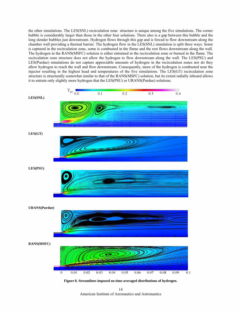
the other simulations. The LES(SNL) recirculation zone structure is unique among the five simulations. The corner bubble is considerably larger than those in the other four solutions. There also is a gap between this bubble and the long slender bubbles just downstream. Hydrogen flows through this gap and is forced to flow downstream along the chamber wall providing a thermal barrier. The hydrogen flow in the LES(SNL) simulation is split three ways. Some is captured in the recirculation zone, some is combusted in the flame and the rest flows downstream along the wall. The hydrogen in the RANS(MSFC) solution is either entrained in the recirculation zone or burned in the flame. The recirculation zone structure does not allow the hydrogen to flow downstream along the wall. The LES(PSU) and LES(Purdue) simulations do not capture appreciable amounts of hydrogen in the recirculation zones nor do they allow hydrogen to reach the wall and flow downstream. Consequently, more of the hydrogen is combusted near the injector resulting in the highest head end temperatures of the five simulations. The LES(GT) recirculation zone structure is structurally somewhat similar to that of the RANS(MSFC) solution, but its extent radially inboard allows it to entrain only slightly more hydrogen that the LES(PSU) or URANS(Purdue) solutions.

LES(SNL)

LES(GT)

LES(PSU)

URANS(Purdue)

RANS(MSFC)

Figure 8. Streamlines imposed on time-averaged distributions of hydrogen.


14

To look more closely at these head end differences, profiles of hydrogen fraction are plotted in Fig. 9 at three axial locations across the recirculation zone (x = 0.0125, 0.025 and 0.05 meters) and at one axial location in the downstream region at x = 0.15 meters. At x = 0.0125 meters, the LES(SNL) and RANS(MSFC) have comparable levels of hydrogen, in the 20% and 15% ranges, respectively. The other three calculations produce significantly lower levels of hydrogen in the 5-9% range. The RANS(MSFC) calculation also exhibits a peak in the hydrogen mass fraction of approximately 26% on the radially outboard side of the flame zone. This is consistent with the observation noted above that the temperature was low here for RANS(MSFC). The similarities in composition and temperature in the recirculation zone (i.e., head end) as the wall is approached for the LES(SNL) and RANS(MSFC) calculations are consistent with the fact that both produced fairly similar predictions for the heat flux in this region. However, the LES(PSU) result has very low hydrogen concentrations in the recirculation zone and the second hottest gas temperatures (as shown in Figs. 3 and 4), yet produces head end heat fluxes similar to the LES(SNL) and RANS(MSFC) results.

x = 0.0125 meters

x = 0.025 meters

x = 0.05 meters

x = 0.15 meters

Figure 9. Radial hydrogen mass fraction profiles at axial locations of 0.0125, 0.025, 0.05 and 0.15 m.

The distributions of hydrogen mass fraction in the entire domain are plotted in Fig. 10. Again, downstream, the

observed over-prediction in the RANS(MSFC) heat flux prediction in region starting at x = 0.1 meters is also consistent with the fact that the hydrogen distribution is markedly different compared to the LES(SNL) result. Figs. 9 and 10 show that the composition of the near wall region downstream at x = 0.15 meters is approximately 16% for the LES(SNL) calculation and this persists along the entire length of the chamber. The RANS(MSFC) case (along with the other three simulations), on the other hand, exhibits levels of hydrogen of less than 3%. The near wall hydrogen in the LES(SNL) case obviously provides a thermal barrier of sorts. However, the URANS(Purdue) calculation has the lowest levels of hydrogen near the wall in the downstream region, but produces a heat flux prediction that is comparable to the LES(SNL) result in this area. While the RANS(MSFC) calculation over predicts the heat flux in the downstream region, the other three calculations with similarly low near-wall hydrogen concentrations under predict the downstream heat flux. These apparent inconsistencies imply the deviations in the heat flux cannot be explained based on the gas temperature fluid composition alone


15

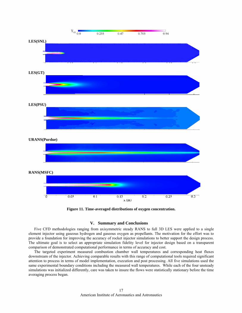
We complete the analysis of the time-average characteristics by examining the distribution of oxygen. To determine the degree to which the oxygen core persists, we have defined an arbitrary cut-off of 10% mass fraction

LES(SNL)

LES(GT)

LES(PSU)

URANS(Purdue)

RANS(MSFC)

Figure 10. Time-averaged distributions of hydrogen mass fraction.

We complete the analysis of the time-average characteristics by examining the distribution of oxygen. To

determine the degree to which the oxygen core persists, we have defined an arbitrary cut-off of 10% mass fraction so that relative comparisons can be made with respect to the core length. Using this definition and Fig. 11, we can identify approximate core lengths of 0.04, 0.06, 0.21, 0.30 and 0.16 meters for the LES(SNL), LES(GT), LES(PSU), URANS(Purdue) and RANS(MSFC) calculations, respectively. The two full 3D LES calculations produce considerably shorter oxygen cores compared to the two 2D axisymmetric calculations. Surprisingly, the URANS(Purdue) calculation produces the longest core, with oxygen exiting through the nozzle, and the 2D LES(PSU) oxygen core is the next longest. The RANS(MSFC) calculation produces a core length of 0.16 meters, which is 50% shorter than the URANS(Purdue) calculation and 30% shorter than the LES(PSU) calculation.


16

LES(SNL)

LES(GT)

LES(PSU)

URANS(Purdue)

RANS(MSFC)

Figure 11. Time-averaged distributions of oxygen concentration.

V. Summary and Conclusions Five CFD methodologies ranging from axisymmetric steady RANS to full 3D LES were applied to a single

element injector using gaseous hydrogen and gaseous oxygen as propellants. The motivation for the effort was to provide a foundation for improving the accuracy of rocket injector simulations to better support the design process. The ultimate goal is to select an appropriate simulation fidelity level for injector design based on a transparent comparison of demonstrated computational performance in terms of accuracy and cost.

The targeted experiment measured combustion chamber wall temperatures and corresponding heat fluxes downstream of the injector. Achieving comparable results with this range of computational tools required significant attention to process in terms of model implementation, execution and post processing. All five simulations used the same experimental boundary conditions including the measured wall temperatures. While each of the four unsteady simulations was initialized differently, care was taken to insure the flows were statistically stationary before the time averaging process began.


17

The results of each simulation were compared to the experimental heat flux data. This LES(SNL) result compared very well with the data. In the context of this effort, the fact the LES(SNL) result yielded the best comparison to the data was not surprising since it was the product of the highest fidelity simulation. In a broader context, it represents the best comparison of all attempts known by the authors. It provides encouraging evidence that these complex injector flow fields can be accurately simulated. However, the enthusiasm is tempered by the fact this simulation was done on a grid with 255x106 cells and required approximately 2 million CPU hours. This level of fidelity is obviously not possible in a production environment. Each of the other four results matched the data reasonably well in certain regions of the chamber, but less well in other regions. There was no monotonic convergence to the experimental data with respect to model fidelity.

This uneven performance of the computational tools required more detailed analysis of the solutions. Since there was no flow field data available front the experiment, two “relative” standards were chosen to facilitate the additional analysis. First, the LES(SNL) simulation represents the state of the art and matched the available data extremely well, so it was used to help gauge the other results. Second, since the MSFC (RANS) simulation represents the state of production, comparison to this result at the opposite end of the fidelity spectrum was useful in understanding its deficiencies. The additional analysis to date consists of examining the details of the temperature fields, OH radical concentration fields, the recirculation zones and the hydrogen and oxygen concentration fields.

The temperature field comparison provided some insight into the heat flux results. First, it showed very different flame structures indicating the mechanisms and rates of mixing and combustion vary significantly among the five simulations. Second, it showed the recirculation zones in the head end were markedly different in terms of size, shape, composition and temperature. Third, it showed the downstream radial temperature distributions varied considerably from the core to the chamber wall. The remaining portion of this section is organized around, and focused on, these three critical areas.

The OH radical and oxygen concentration fields provided additional information on the structure of the flame zone. The OH field showed the RANS(MSFC) had by far the most distinct flame zone which was defined by a continuous flame sheet that bounded the oxygen core ending about two-thirds of the way down the chamber. The other four solutions exhibited much more diffuse flame zones. The LES(SNL) simulation burned much less intensely, but continued to burn through the end of the chamber. The LES(GT) result showed slightly more intense burning than the LES(SNL) solution, but in a very localized region along the centerline in the head end. The 2D unsteady simulations, LES(PSU) and URANS(Purdue), had the most diffuse flame zones as evidenced by the high temperatures across the chamber starting in the far head end. They were also unique in that the centerline temperatures stayed relatively cool down the entire chamber. The oxygen core information supports these observations. Notably, the centerline oxygen concentration in the LES(PSU) and URANS(Purdue) solutions extended very far down the chamber; even through the chamber exit in the case of URANS(Purdue).

The distinct, intense RANS(MSFC) flame was almost certainly caused by the assumptions that the flow is steady and axisymmetric. Given these two assumptions, the vortical mixing mechanism seen in the four unsteady solutions is impossible. The very diffuse flame zones and the persistence of oxygen on the centerline downstream shown by the LES(PSU) and URANS(Purdue) solutions were likely the product of the 2D axisymmetric assumption. The 3D LES solutions produced smaller structures but had less disperse flame zones than the other unsteady simulations.

The recirculation zone structure, in terms of size, shape and location has a very significant impact on the head end heat gas composition, and thus, heat flux. The LES(SNL) recirculation zone was distinct in that it not only captured hydrogen, but also pulled some of the hydrogen outboard to the wall where it flowed down the entire chamber length. The RANS(MSFC) recirculation zone had approximately the same hydrogen concentration, but, since it was larger, actually contained more hydrogen mass. The LES(GT), LES(PSU) and URANS(Purdue) recirculation zone capture very little hydrogen. The amount of hydrogen entrained in the recirculation zone seems to be a function of the proximity of the inboard boundary of the bubble relative to the hydrogen inlet. The LES(GT), LES(PSU) and URANS(Purdue) recirculation zones have similar low hydrogen concentrations in their respective recirculation zones, but the URANS(Purdue) solution over predicts the head end heat flux while the other two solutions under predict it. This observation provides another seeming conflict at this level of analysis.

Finally, looking at the downstream region of the combustion chamber, the LES(SNL) solution was significantly cooler in the near wall region due to hydrogen concentrations that were 5-10 times higher than those in the other four solutions. However, the downstream heat flux values here were inconsistent in that the LES(SNL) and URANS(Purdue) solutions compared very well with the data, the LES(GT) solution under predicted the data and the LES(PSU) solution under predicted and then over predicted the data. The RANS(MSFC) hydrogen-rich recirculation zone ended at about x=0.10 meters coinciding with the subsequent over prediction of the downstream heat flux.


18

There are significant inconsistencies in the evaluation of the five simulations that are not reconcilable with this level of analysis. However, at a higher level, the answer to the question of how to affordably improve the accuracy of CFD simulations for injector design is becoming somewhat clearer. First, this effort has shown that the steady assumption for injector flows precludes critical mixing mechanisms. Since injector flows are mixing dominated, this is a very serious limitation. In terms of accurate heat flux predictions, it seems that any credible simulation must be time accurate. Relative to the RANS(MSFC) simulation, the first progression in fidelity is represented by the URANS(Purdue) simulation. This step increases the computational cost by a factor of approximately 15, based on a comparison of the RANS(MSFC) and URANS(Purdue) CPU times. If four weeks is set as the maximum turn around time to support the design cycle, the URANS(Purdue) simulation requires just under 40 CPUs. At this level, a limited set of parametric analyses could be executed during the design cycle.

This work has also identified some apparent shortcomings of the time accurate simulations using the 2D axisymmetric assumption. Unsteady flows are inherently three dimensional. Although worrisome, it is not yet totally clear how limiting the symmetry constraint is in the injector problem. If it is shown that the accuracy of 3D simulations is required to support injector design, that represents at least another factor of 10 increase in computational cost. Today, this is problematic in the design environment.

Future Work In terms of the overall effort, more detailed analysis of the Element 1 results is required along with completion

of similar work on Elements 2 and 3. For Element 1, the required additional work consists of 1) evaluation of the axial distribution of thermal conductivity and wall temperature gradients, 2) assessment of the velocity, thermal and mass boundary layers to understand differences in both the steady and unsteady boundary layer characteristics and 3) understanding the requirements and methods used by each tool to determine heat flux.

Acknowledgments This work is a result of a large group of co-workers including Doug Westra, Jeff Lin and Jeff West at NASA

Marshall Space Flight Center; Matthieu Masquelet and Orcun Kozaka at the Georgia Institute of Technology; Chenzhou Lian and Guoping Xia at Purdue University; and Nan Zong at The Pennsylvania State University. The authors would like to acknowledge financial support from the Constellation University Institutes Program (CUIP). CUIP is funded by NASA Headquarters and managed at NASA Glenn Research Center by Claudia Meyer and Jeff Rybak. Funding was also supplied from the Space Shuttle Main Engine Office at NASA Marshall Space Flight Center by Carol Jacobs.

References 1Tucker, P. K., Menon, S., Merkle, C. L., Oefelein, J. C. And Yang, V.,”An Approach to Improved Credibility of CFD

Simulations fro Rocket Injector Design,” AIAA Paper No. 2007-5572, July, 2007. 2West, J., Westra, D., Lin, J. and Tucker, K., “Accuracy Quantification of the Loci-CHEM Code for Chamber Wall Heat

Fluxes in a GO2/GH2 Single Element Injector Model Problem,” Third International Workshop on Rocket Combustion Modeling, Paris, France, March 13-15, 2006.

3West, J., Lin, J., Tucker, K. and Chenoweth, J., “Steady State Combustion CFD Analysis of Local Heat Transfer for Liquid Oxygen/Gaseous Hydrogen Injectors,” 53rd JANNAF Propulsion Meeting/2nd Liquid Propulsion Subcommittee Meeting, December 5-8, 2005.

4Pal, S., Marshall, W., Woodward, R. and Santoro, R., “Wall Heat Flux Measurements for a Uni-element GO2/GH2 Shear Coaxial Injector,” Third International Workshop on Rocket Combustion Modeling, Paris, France, March 13-15, 2006.

5Oefelein, J. C., “Large eddy simulation of turbulent combustion processes in propulsion and power systems,” Progress in Aerospace Sciences, Vol. 42, 2006, pp. 2-37.

6Oefelein, J. C., “Mixing and combustion of cryogenic oxygen-hydrogen shear-coaxial jet flames at supercritical pressure,” Combustion Science and Technology, Vol. 178, No. 1-3, 2006, pp. 229-252.

7Oefelein, J. C., “Thermophysical characteristics of LOX-H2 flames at supercritical pressure,” Proceedings of the Combustion Institute, Vol. 30, 2005, pp. 2929-2937.

8Pantano, C. and Sarkar, S., “A subgrid model for nonlinear functions of a scalar,” Physics of Fluids, Vol. 13, No. 12, 2001, pp. 3803-3819.

9Mellado, J. P., Sarkar, S., and Pantano, C., “Reconstruction subgrid models for nonpremixed combustion,” Physics of Fluids, Vol. 15, No. 11, 2003, pp. 3280-3307.

10Ó Conaire, M., Curran, H. J., Simmie, J. M., Pitz, W. J. and Westbrook, C. K., “A comprehensive modeling study of hydrogen oxidation,” International Journal of Chemical Kinetics, Vol. 36, 2004, pp. 603-622.


19

11Genin, F., Fryxell, B. and Menon, S., “Hybrid Large-Eddy Simulation of Detonation in Reactive Mixtures,” Proceedings of the 20th International Conference on Detonations, Explosions and Shock Waves, Montreal CA, August 1-4, 2005.

12Masquelet, M. and Menon, S., “Large Eddy Simulation of Flame-Turbulence Interactions in a GH2-GO2 Shear Coaxial Injector,” AIAA-2008-5030, 44th AIAA/ASME/SAE/ASEE Joint Propulsion Conference and Exhibit, 2008.

13Meng, H., and Yang, V., “A Unified Treatment of General Fluid Thermodynamics and Its Application to a Preconditioning Scheme,” J. Comput. Phys., Vol. 189, 2003, pp. 277-304.

14Meng, H., Hsiao, G.C., Yang, V., and Shuen, J. S., “Transport and Dynamics of Liquid Oxygen Droplets in Supercritical Hydrogen Streams,” J. Fluid Mech., Vol. 527, 2005, pp. 115-139.

15Zong, N., Meng, H., Hsieh, S.Y., and Yang, V., “A Numerical Study of Cryogenic Fluid Injection and Mixing under Supercritical Conditions,” Phys. Fluids, Vol. 16, 2004, pp. 4248-4261.

16Yang V., “Modeling of Supercritical Vaporization, Mixing and Combustion Processes in Liquid-Fueled Propulsion Systems. Proc. Combust. Inst., Vol. 28, 2000, pp. 925–942.

17Ribert, G., Zong, N., and Yang, V., “Counterflow Diffusion Flames of General Fluids: Oxygen/Hydrogen Mixtures,” AIAA Paper No. 2007-1427, 2007.

18Hsieh, S.Y., and Yang, V., “A Preconditioned Flux-Differencing Scheme for Chemically Reacting Flows at All Mach Numbers,” Int. J. Comput. Fluid Dyn., Vol. 8, 1997, pp. 31-49.

19Zong, N., and Yang, V., “A efficient preconditioning scheme for real fluid mixtures using primitive pressure-temperature variables,” submitted to Int. J. Comput. Fluid Dyn., 2007.

20Zong, N., Ribert, G., and Yang, V., “Supercritical Combustion of Liquid Oxygen (LOX) and Methane Stabilized by a Splitter Plate” AIAA Paper No. 2007-0575, 2007.

21Venkateswaran, S., Merkle, C. L., Zeng, X and Li, D., “Influence of Large-Scale Pressure Changes on Pre-Conditioned Solutions at Low Speeds,” AIAA Journal, Vol. 42, No. 12, 2004, pp 2490-2498.

22Li, D., Xia, G. and Merkle, C. L., “Analysis of Real Fluid Flows in Converging Diverging Nozzles,” AIAA Paper 2003-4132, 33rd AIAA Fluid Dynamics Conference and Exhibit, Orlando, Florida, June 23-26, 2003.

23Luke, E. A., Tong, X.-L. and Cinnella, P. “Numerical Simulations of Fluids with a General Equation of State”, AIAA 2006-12951 44th Aerospace Sciences Meeting, January 9-12, 2006, Reno, NV.

24Luke, E. A., Tong, X.-L., Wu, J. and Cinella, P., “CHEM 2: A Finite-Rate Viscous Chemistry Solver – The User Guide,” MSSU-COE-ERC-04-07, Mississippi State University, September, 2004.

25Luke, E. A., “A Rule-Based Specification System for Computational Fluid Dynamics,” Ph.D. Dissertation, Mississippi State University, Starkville, MS, 1999.

26Menter, F. R., “Two-Equation Eddy-Viscosity Turbulence Models for Engineering Applications,” AIAA Journal, Vol. 32, No. 8, 1994, pp. 1598-1605.

28Evans. J. S. and Schexnayder, C. J., “Influence of Chemical Kinetics and Unmixedness on Burning in Supersonic Hydrogen Flames,” AIAA Journal, Vol 18, No 2, 1980, pp. 188-193.

29Gridgen, Software Package, Version 15, Pointwise, Inc., Bedford, Texas, 2005.


20

Documents

Validation of High-Fidelity CFD Simulations for Rocket Injector Design … · 2013-04-10 · Validation of High-Fidelity CFD Simulations for Rocket Injector Design P. Kevin Tucker1