Validation of GOES-R Satellite Land Surface Temperature Algorithm Using SURFRAD Ground Measurements and Statistical Estimates of Error Properties

704 IEEE TRANSACTIONS ON GEOSCIENCE AND REMOTE SENSING, VOL. 50, NO. 3, MARCH 2012

Validation of GOES-R Satellite Land SurfaceTemperature Algorithm Using SURFRAD

Ground Measurements and StatisticalEstimates of Error Properties

Yunyue Yu, Dan Tarpley, Jeffrey L. Privette, Lawrence E. Flynn, Hui Xu,Ming Chen, Konstantin Y. Vinnikov, Donglian Sun, and Yuhong Tian

Abstract—Validation of satellite land surface temperature(LST) is a challenge because of spectral, spatial, and temporalvariabilities of land surface emissivity. Highly accurate in situ LSTmeasurements are required for validating satellite LST productsbut are very hard to obtain, except at discrete points or for veryshort time periods (e.g., during field campaigns). To comparethese field-measured point data with moderate-resolution (∼1 km)satellite products requires a scaling process that can introduce er-rors that ultimately exceed those in the satellite-derived LST prod-ucts whose validation is sought. This paper presents a new methodof validating the Geostationary Operational Environmental Satel-lite (GOES) R-Series (GOES-R) Advanced Baseline Imager (ABI)LST algorithm. It considers the error structures of both groundand satellite data sets. The method applies a linear fitting modelto the satellite data and coregistered “match-up” ground data forestimating the precisions of both data sets. In this paper, GOES-8Imager data were used as a proxy of the GOES-R ABI data forthe satellite LST derivation. The in situ data set was obtained fromthe National Oceanic and Atmospheric Administration’s SURFaceRADiation (SURFRAD) budget network using a stringentmatch-up process. The data cover one year of GOES-8 Imagerobservations over six SURFRAD sites. For each site, more than1000 cloud-free match-up data pairs were obtained for day andnight to ensure statistical significance. The average precision overall six sites was found to be 1.58 K, as compared to the GOES-RLST required precision of 2.3 K. The least precise comparison atan individual SURFRAD site was 1.8 K. The conclusion is that, for

Manuscript received December 9, 2010; revised March 11, 2011 and June 20,2011; accepted June 27, 2011. Date of publication August 22, 2011; date ofcurrent version February 24, 2012. This work was supported by the ApplicationWorking Group, Geostationary Operational Environmental Satellite R-Series,National Oceanic and Atmospheric Administration.

Y. Yu and L. E. Flynn are with the Center for Satellite Applications andResearch, National Environmental Satellite, Data, and Information Service,National Oceanic and Atmospheric Administration, Camp Springs, MD 20746USA (e-mail: [email protected]; [email protected]).

D. Tarpley is with Short and Associates, Camp Springs, MD 20746 USA(e-mail: [email protected]).

J. L. Privette is with the National Climatic Data Center, National En-vironmental Satellite, Data, and Information Service, National Oceanic andAtmospheric Administration, Asheville, NC 28801 USA (e-mail: [email protected]).

H. Xu, M. Chen, and Y. Tian are with I. M. Systems Group, Inc., CampSprings, MD 20746 USA (e-mail: [email protected]; [email protected];[email protected]).

K. Y. Vinnikov is with the Department of Atmospheric and Oceanic Science,University of Maryland, College Park, MD 20742 USA (e-mail: [email protected]).

D. Sun is with the Department of Geography and Geoinformation Science,George Mason University, Fairfax, VA 22030 USA (e-mail: [email protected]).

Digital Object Identifier 10.1109/TGRS.2011.2162338

these ground truth sites, the GOES-R LST algorithm meets thespecifications and that an upper boundary on the precision of thesatellite LSTs can be determined.

Index Terms—Algorithm evaluation, land surface temperature(LST), satellite measurement, SURFace RADiation (SURFRAD).

I. INTRODUCTION

IN THE DEVELOPMENT and use of satellite land surfacetemperature (LST) retrieval algorithms, validation is crucial

yet difficult. Validation provides the quantitative uncertaintyinformation required for the proper use and application of theproduct. No algorithm or product would be widely acceptedwithout performing thorough calibration and validation. Tra-ditionally, satellite LST validation is performed by comparingthe satellite-derived LST to ground, aircraft, or other satelliteLST estimates; both real and simulated satellite and grounddata have been used. For instance, Wan et al. [1] performeddirect and indirect validations of the LST product retrievedfrom Earth Observation System MODerate-resolution ImagingSpectroradiometer (MODIS) data using ground data collectedfrom several field campaigns. Coll et al. [2] conducted a fieldcampaign over a large, flat, and homogeneous rice crop area forvalidation of LST products derived from MODIS and EuropeanSpace Agency Environmental Satellite Advanced Along-TrackScanning Radiometer data. Yu et al. [3] applied their evaluationresults to the LST algorithms for Visible and Infrared Image Ra-diometer Suite of the National Polar-orbiting Operational Envi-ronmental Satellite System using a comprehensive simulationdata set and MODIS data. Pinheiro et al. [4] validated nonnadirAdvanced Very High Resolution Radiometer LST estimatesover Africa using field measurements combined with an angularemission model. Vinnikov et al. [5] evaluated the satellite LSTsfrom the LST diurnal variation feature derived from Geostation-ary Operational Environmental Satellite (GOES) Imager data.

There are many challenges in such direct comparisons ofLST algorithms and products, including the following.

1) The land surface is typically heterogeneous (both in tem-perature and emissivity) over satellite pixel areas (e.g.,∼1 km), while in situ LST measurements are usually col-lected over significantly smaller and more homogeneousareas (e.g., ∼0.01 km).

0196-2892/$26.00 © 2011 IEEE

YU et al.: VALIDATION OF LST ALGORITHM USING GROUND MEASUREMENTS AND ESTIMATES OF ERROR 705

2) Navigation errors cause the ground truth site to movefrom place to place within the coincident pixel, and in1%–2% of pixels, the ground site may be outside the “co-incident” pixel. A navigation uncertainty is a significantsource of imprecision.

3) Accurate fine-resolution land surface emissivity data areneeded but hard to obtain.

4) The rate of LST change is usually high, so the time dif-ferences between satellite LST and ground measurementmust be relatively small.

5) There are few field sites where in situ LST data areroutinely or episodically measured.

6) Cloud contamination in satellite data may have significantnegative impacts on the validation process.

7) Angular anisotropy (directional variability) of apparentsurface emissivity and temperature has significant impacton the LST retrieval.

For these reasons, collecting and processing highly accurateground measurements that match the satellite LST measure-ments can be a tedious and costly task.

Given these challenges, it is important to quantify the un-certainty (accuracy and precision) of the properly scaled inde-pendent “validation data set” as part of the validation process.Flynn [6] described a statistical method for validating satellitesounding products. Instead of directly comparing the satellite-derived and in situ measurement data (e.g., scatterplots with areference line and histogram of difference), he explored proce-dures for simultaneously estimating possible errors from boththe satellite data and ground measurements. His approach canhelp quantify validation results and improve their interpretation.

In this paper, we applied Flynn’s method to estimate errorsin LST derived from the U.S. GOES Imager data. Our goal isto evaluate the baseline LST algorithm for the new AdvancedBaseline Imager (ABI) instrument that will fly on a new gen-eration of GOES satellites, i.e., the GOES R-Series (GOES-R)[7]. In the following section, we provide details of the data setsused in this study. Section III gives the theoretical fundamentalsand derived equations. We then show the results in Section IV,followed by a discussion of results in Section V. Finally, weprovide some concluding remarks in Section VI.

II. DATA SETS

Two data sets were used in this study: SURFace RADia-tion (SURFRAD) ground measurements and GOES-8 Imagerdata. We created a set of coregistered “match-up” LST dataderived from GOES-8 Imager and ground measurements fromthe SURFRAD budget network stations. We then used Flynn’smethod to evaluate satellite measurements in relation to in situmeasurements and to estimate the errors and consistency of thesatellite LSTs under a variety of scenarios.

A. SURFRAD Data

The SURFRAD network has been operational in the U.S.since 1995. It provides high-quality in situ measurements ofupwelling and downwelling radiative fluxes, along with othermeteorological parameters [8]. In this paper, we used one year

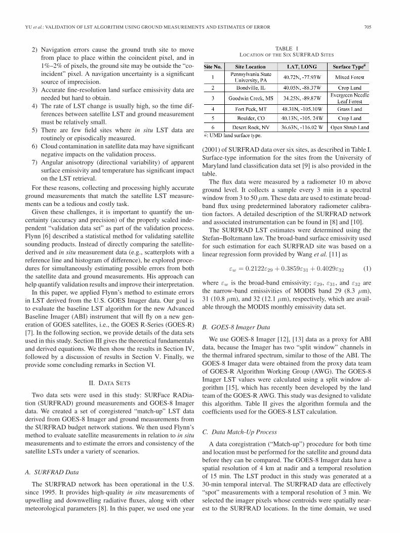
TABLE ILOCATION OF THE SIX SURFRAD SITES

(2001) of SURFRAD data over six sites, as described in Table I.Surface-type information for the sites from the University ofMaryland land classification data set [9] is also provided in thetable.

The flux data were measured by a radiometer 10 m aboveground level. It collects a sample every 3 min in a spectralwindow from 3 to 50 μm. These data are used to estimate broad-band flux using predetermined laboratory radiometer calibra-tion factors. A detailed description of the SURFRAD networkand associated instrumentation can be found in [8] and [10].

The SURFRAD LST estimates were determined using theStefan–Boltzmann law. The broad-band surface emissivity usedfor such estimation for each SURFRAD site was based on alinear regression form provided by Wang et al. [11] as

εw = 0.2122ε29 + 0.3859ε31 + 0.4029ε32 (1)

where εw is the broad-band emissivity; ε29, ε31, and ε32 arethe narrow-band emissivities of MODIS band 29 (8.3 μm),31 (10.8 μm), and 32 (12.1 μm), respectively, which are avail-able through the MODIS monthly emissivity data set.

B. GOES-8 Imager Data

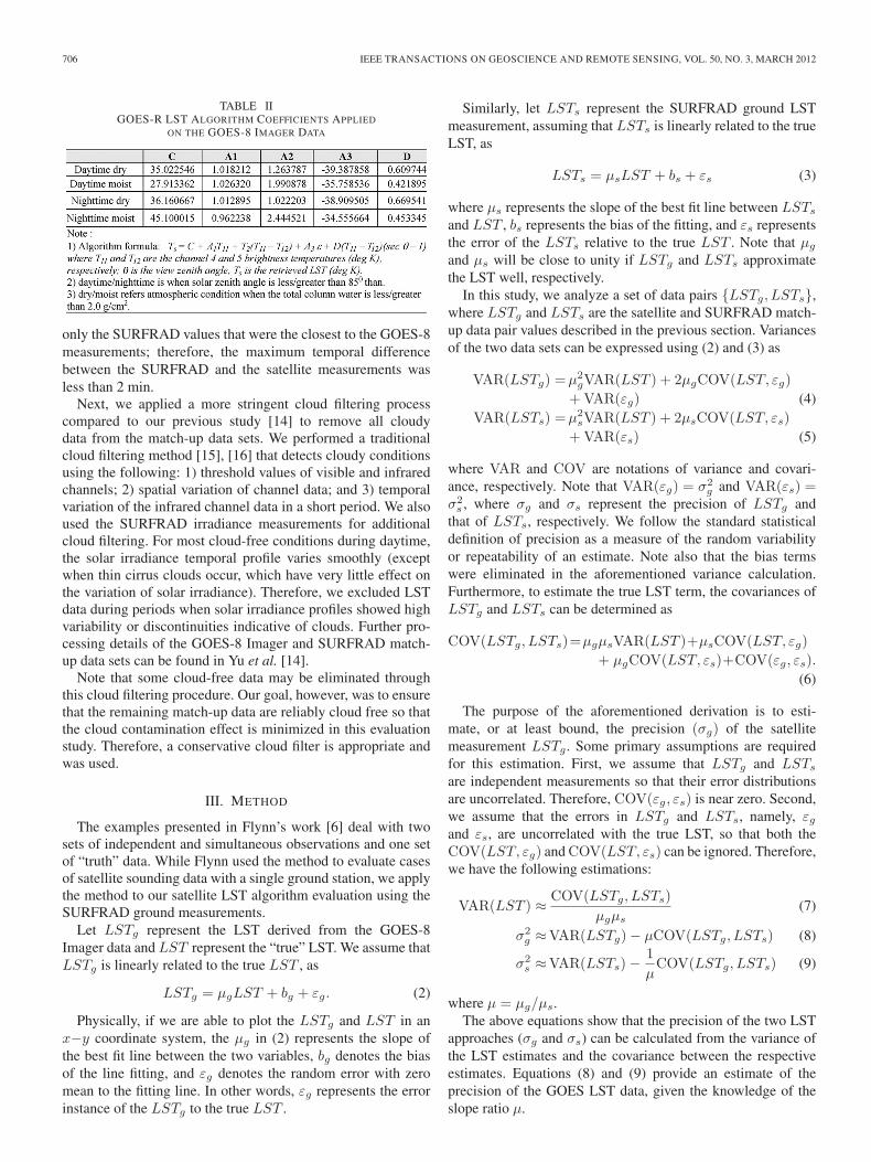
We use GOES-8 Imager [12], [13] data as a proxy for ABIdata, because the Imager has two “split window” channels inthe thermal infrared spectrum, similar to those of the ABI. TheGOES-8 Imager data were obtained from the proxy data teamof GOES-R Algorithm Working Group (AWG). The GOES-8Imager LST values were calculated using a split window al-gorithm [15], which has recently been developed by the landteam of the GOES-R AWG. This study was designed to validatethis algorithm. Table II gives the algorithm formula and thecoefficients used for the GOES-8 LST calculation.

C. Data Match-Up Process

A data coregistration (“Match-up”) procedure for both timeand location must be performed for the satellite and ground databefore they can be compared. The GOES-8 Imager data have aspatial resolution of 4 km at nadir and a temporal resolutionof 15 min. The LST product in this study was generated at a30-min temporal interval. The SURFRAD data are effectively“spot” measurements with a temporal resolution of 3 min. Weselected the imager pixels whose centroids were spatially near-est to the SURFRAD locations. In the time domain, we used


TABLE IIGOES-R LST ALGORITHM COEFFICIENTS APPLIED

ON THE GOES-8 IMAGER DATA

only the SURFRAD values that were the closest to the GOES-8measurements; therefore, the maximum temporal differencebetween the SURFRAD and the satellite measurements wasless than 2 min.

Next, we applied a more stringent cloud filtering processcompared to our previous study [14] to remove all cloudydata from the match-up data sets. We performed a traditionalcloud filtering method [15], [16] that detects cloudy conditionsusing the following: 1) threshold values of visible and infraredchannels; 2) spatial variation of channel data; and 3) temporalvariation of the infrared channel data in a short period. We alsoused the SURFRAD irradiance measurements for additionalcloud filtering. For most cloud-free conditions during daytime,the solar irradiance temporal profile varies smoothly (exceptwhen thin cirrus clouds occur, which have very little effect onthe variation of solar irradiance). Therefore, we excluded LSTdata during periods when solar irradiance profiles showed highvariability or discontinuities indicative of clouds. Further pro-cessing details of the GOES-8 Imager and SURFRAD match-up data sets can be found in Yu et al. [14].

Note that some cloud-free data may be eliminated throughthis cloud filtering procedure. Our goal, however, was to ensurethat the remaining match-up data are reliably cloud free so thatthe cloud contamination effect is minimized in this evaluationstudy. Therefore, a conservative cloud filter is appropriate andwas used.

III. METHOD

The examples presented in Flynn’s work [6] deal with twosets of independent and simultaneous observations and one setof “truth” data. While Flynn used the method to evaluate casesof satellite sounding data with a single ground station, we applythe method to our satellite LST algorithm evaluation using theSURFRAD ground measurements.

Let LSTg represent the LST derived from the GOES-8Imager data and LST represent the “true” LST. We assume thatLSTg is linearly related to the true LST , as

LSTg = μgLST + bg + εg. (2)

Physically, if we are able to plot the LSTg and LST in anx−y coordinate system, the μg in (2) represents the slope ofthe best fit line between the two variables, bg denotes the biasof the line fitting, and εg denotes the random error with zeromean to the fitting line. In other words, εg represents the errorinstance of the LSTg to the true LST .

Similarly, let LSTs represent the SURFRAD ground LSTmeasurement, assuming that LSTs is linearly related to the trueLST, as

LSTs = μsLST + bs + εs (3)

where μs represents the slope of the best fit line between LSTs

and LST , bs represents the bias of the fitting, and εs representsthe error of the LSTs relative to the true LST . Note that μg

and μs will be close to unity if LSTg and LSTs approximatethe LST well, respectively.

In this study, we analyze a set of data pairs {LSTg, LSTs},where LSTg and LSTs are the satellite and SURFRAD match-up data pair values described in the previous section. Variancesof the two data sets can be expressed using (2) and (3) as

VAR(LSTg) =μ2gVAR(LST ) + 2μgCOV(LST, εg)

+ VAR(εg) (4)VAR(LSTs) =μ2

sVAR(LST ) + 2μsCOV(LST, εs)

+ VAR(εs) (5)

where VAR and COV are notations of variance and covari-ance, respectively. Note that VAR(εg) = σ2

g and VAR(εs) =σ2s , where σg and σs represent the precision of LSTg and

that of LSTs, respectively. We follow the standard statisticaldefinition of precision as a measure of the random variabilityor repeatability of an estimate. Note also that the bias termswere eliminated in the aforementioned variance calculation.Furthermore, to estimate the true LST term, the covariances ofLSTg and LSTs can be determined as

COV(LSTg, LSTs)=μgμsVAR(LST )+μsCOV(LST, εg)

+ μgCOV(LST, εs)+COV(εg, εs).

(6)

The purpose of the aforementioned derivation is to esti-mate, or at least bound, the precision (σg) of the satellitemeasurement LSTg . Some primary assumptions are requiredfor this estimation. First, we assume that LSTg and LSTs

are independent measurements so that their error distributionsare uncorrelated. Therefore, COV(εg, εs) is near zero. Second,we assume that the errors in LSTg and LSTs, namely, εgand εs, are uncorrelated with the true LST, so that both theCOV(LST, εg) and COV(LST, εs) can be ignored. Therefore,we have the following estimations:

VAR(LST ) ≈ COV(LSTg, LSTs)

μgμs(7)

σ2g ≈VAR(LSTg)− μCOV(LSTg, LSTs) (8)

σ2s ≈VAR(LSTs)−

1

μCOV(LSTg, LSTs) (9)

where μ = μg/μs.The above equations show that the precision of the two LST

approaches (σg and σs) can be calculated from the variance ofthe LST estimates and the covariance between the respectiveestimates. Equations (8) and (9) provide an estimate of theprecision of the GOES LST data, given the knowledge of theslope ratio μ.


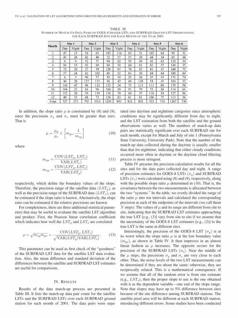
TABLE IIINUMBER OF MATCH-UP DATA PAIRS OF GOES-8 IMAGER LSTs AND SURFRAD GROUND LST OBSERVATIONS,

FOR EACH SURFRAD SITE FOR EACH MONTH OF THE YEAR 2001

In addition, the slope ratio μ is constrained by (8) and (9),since the precisions σg and σs must be greater than zero.That is

μ =μg

μs∈[mgs,

1

msg

](10)

where

mgs =COV(LSTg, LSTs)

VAR(LSTs)(11)

msg =COV(LSTg, LSTs)

VAR(LSTg)(12)

respectively, which define the boundary values of the slope.Therefore, the precision range of the satellite data (LSTg), aswell as the precision range of the SURFRAD data (LSTs), canbe estimated if the slope ratio is known. Alternatively, the sloperatio can be estimated if the relative precisions are known.

For completeness, there are three additional statistical param-eters that may be useful to evaluate the satellite LST algorithmand product. First, the Pearson linear correlation coefficientwhich indicates how well the LSTg and LSTs are correlated

ρ =√msgmgs =

COV(LSTg, LSTs)√VAR(LSTg)VAR(LSTs)

. (13)

This parameter can be used as first check of the “goodness”of the SURFRAD LST data for the satellite LST data evalua-tion. Also, the mean difference and standard deviation of thedifferences between the satellite and SURFRAD LST estimatesare useful for comparisons.

IV. RESULTS

Results of the data match-up process are presented inTable III. It lists the match-up data pair count for the satelliteLSTs and the SURFRAD LSTs over each SURFRAD groundstation for each month of 2001. The data pairs were sepa-

rated into daytime and nighttime categories since atmosphericconditions may be significantly different from day to night,and the LST estimation from both the satellite and the groundobservations varies as well. The numbers of match-up datapairs are statistically significant over each SURFRAD site foreach month, except for March and July of site 1 (PennsylvaniaState University, University Park). Note that the number of thematch-up data collected during the daytime is usually smallerthan that for nighttime, indicating that either cloudy conditionsoccurred more often in daytime or the daytime cloud filteringprocess is more stringent.

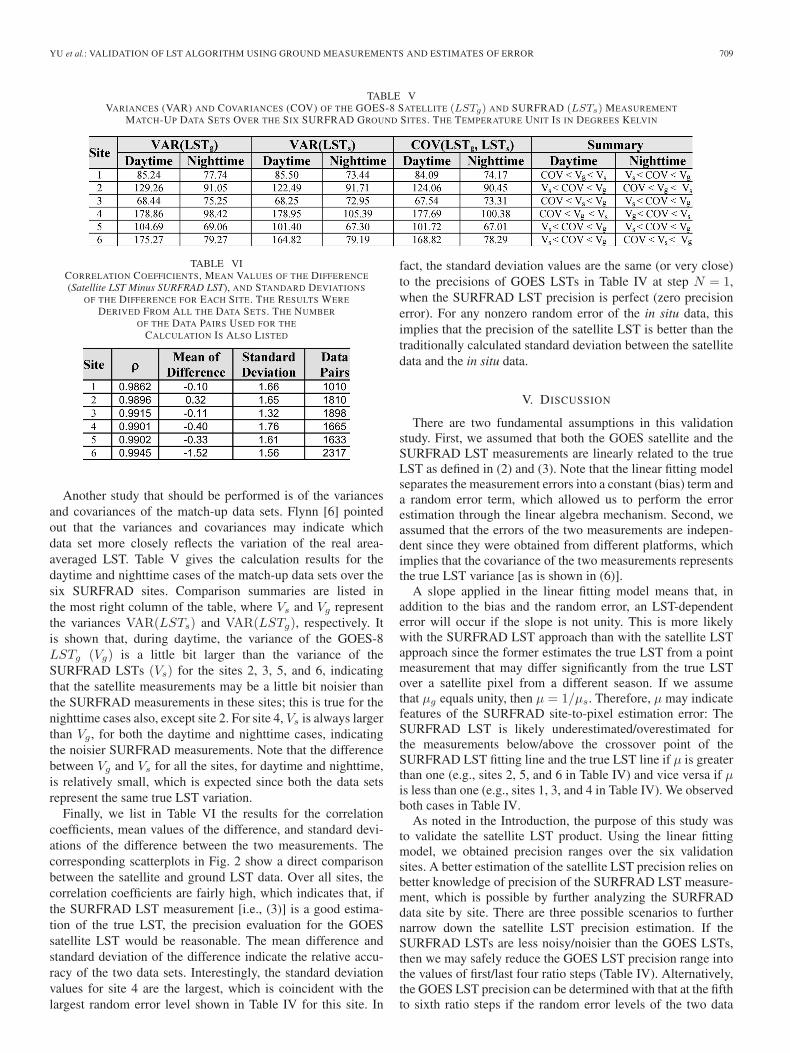
Table IV presents the precision calculation results for all thesites and for the data pairs collected day and night. A rangeof precision estimates for GOES-8 LSTs (σg) and SURFRADLSTs (σs) were calculated using (8) and (9), respectively, alongwith the possible slope ratio μ determined in (10). That is, thecovariance between the two measurements is allocated betweenthe two “systems.” In the table, we evenly divided the range ofthe ratio μ into ten intervals and calculated the correspondingprecision at each of the endpoints of the intervals (we call themN steps). The values of μ and its range are different from site tosite, indicating that the SURFRAD LST estimates approachingthe true LST [e.g., (3)] vary from site to site if we assume thatthe uncertainty of the GOES-8 LST estimates [e.g., (2)] to thetrue LST is the same at different sites.

Interestingly, the precision of the GOES-8 LST (σg) is atits worst when the slope ratio μ is at the low boundary value(mgs), as shown in Table IV. It then improves in an almostlinear fashion as μ increases. The opposite occurs for theprecision of the SURFRAD LSTs (σs). Near the middle ofthe μ steps, the precisions σg and σs are very close to eachother. Thus, the noise levels of the two LST measurements canbe determined if they are about the same; otherwise, they arereciprocally related. This is a mathematical consequence. Ifwe assume that all of the random error is from one estimate(e.g., LSTs), then the proper slope to use is the one obtainedwith it as the dependent variable—one end of the slope range.Note that slopes may have up to 5% difference between sitesbecause of the site difference among SURFRAD stations. Thesatellite pixel area will be different at each SURFRAD station,introducing different errors. Some studies have been conducted


TABLE IVPRECISION (IN DEGREES KELVIN) OF THE SATELLITE LST MEASUREMENTS (σg) AND SURFRAD LST MEASUREMENTS (σs), FROM THE

SIX SURFRAD SITE MATCH-UP DATA SETS. A RANGE OF SLOPES μ IS DETERMINED BY USING (9) FOR EACH SITE, AND IT WAS EVENLY

DIVIDED INTO TEN INTERVALS (N = 1, . . . , 11) FOR THE PRECISION CALCULATIONS. THE RESULTS WERE DERIVED FROM ALL THE DATA SETS

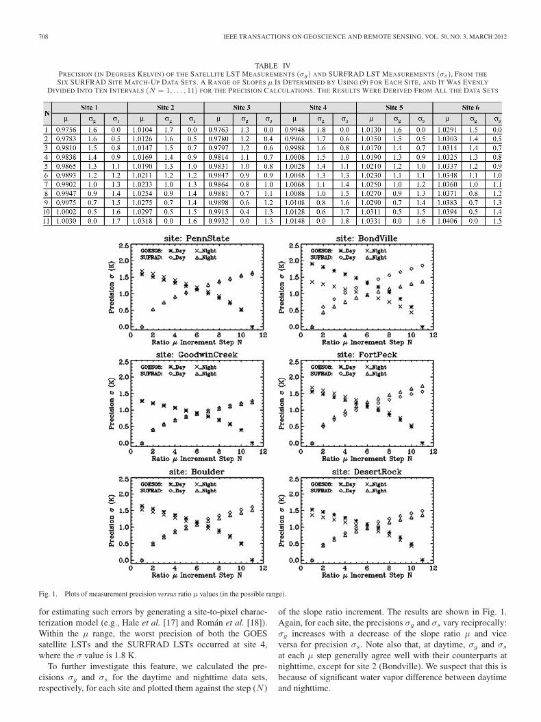
Fig. 1. Plots of measurement precision versus ratio μ values (in the possible range).

for estimating such errors by generating a site-to-pixel charac-terization model (e.g., Hale et al. [17] and Román et al. [18]).Within the μ range, the worst precision of both the GOESsatellite LSTs and the SURFRAD LSTs occurred at site 4,where the σ value is 1.8 K.

To further investigate this feature, we calculated the pre-cisions σg and σs for the daytime and nighttime data sets,respectively, for each site and plotted them against the step (N )

of the slope ratio increment. The results are shown in Fig. 1.Again, for each site, the precisions σg and σs vary reciprocally:σg increases with a decrease of the slope ratio μ and viceversa for precision σs. Note also that, at daytime, σg and σs

at each μ step generally agree well with their counterparts atnighttime, except for site 2 (Bondville). We suspect that this isbecause of significant water vapor difference between daytimeand nighttime.


TABLE VVARIANCES (VAR) AND COVARIANCES (COV) OF THE GOES-8 SATELLITE (LSTg) AND SURFRAD (LSTs) MEASUREMENT

MATCH-UP DATA SETS OVER THE SIX SURFRAD GROUND SITES. THE TEMPERATURE UNIT IS IN DEGREES KELVIN

TABLE VICORRELATION COEFFICIENTS, MEAN VALUES OF THE DIFFERENCE

(Satellite LST Minus SURFRAD LST), AND STANDARD DEVIATIONS

OF THE DIFFERENCE FOR EACH SITE. THE RESULTS WERE

DERIVED FROM ALL THE DATA SETS. THE NUMBER

OF THE DATA PAIRS USED FOR THE

CALCULATION IS ALSO LISTED

Another study that should be performed is of the variancesand covariances of the match-up data sets. Flynn [6] pointedout that the variances and covariances may indicate whichdata set more closely reflects the variation of the real area-averaged LST. Table V gives the calculation results for thedaytime and nighttime cases of the match-up data sets over thesix SURFRAD sites. Comparison summaries are listed inthe most right column of the table, where Vs and Vg representthe variances VAR(LSTs) and VAR(LSTg), respectively. Itis shown that, during daytime, the variance of the GOES-8LSTg (Vg) is a little bit larger than the variance of theSURFRAD LSTs (Vs) for the sites 2, 3, 5, and 6, indicatingthat the satellite measurements may be a little bit noisier thanthe SURFRAD measurements in these sites; this is true for thenighttime cases also, except site 2. For site 4, Vs is always largerthan Vg , for both the daytime and nighttime cases, indicatingthe noisier SURFRAD measurements. Note that the differencebetween Vg and Vs for all the sites, for daytime and nighttime,is relatively small, which is expected since both the data setsrepresent the same true LST variation.

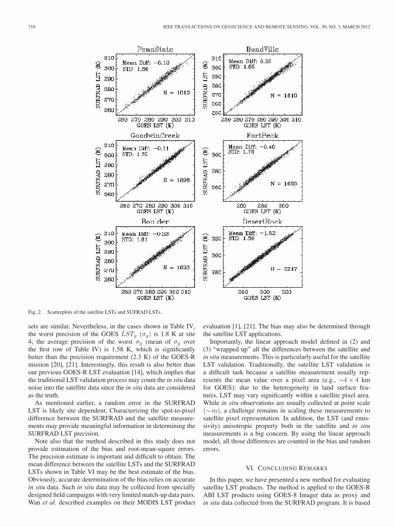
Finally, we list in Table VI the results for the correlationcoefficients, mean values of the difference, and standard devi-ations of the difference between the two measurements. Thecorresponding scatterplots in Fig. 2 show a direct comparisonbetween the satellite and ground LST data. Over all sites, thecorrelation coefficients are fairly high, which indicates that, ifthe SURFRAD LST measurement [i.e., (3)] is a good estima-tion of the true LST, the precision evaluation for the GOESsatellite LST would be reasonable. The mean difference andstandard deviation of the difference indicate the relative accu-racy of the two data sets. Interestingly, the standard deviationvalues for site 4 are the largest, which is coincident with thelargest random error level shown in Table IV for this site. In

fact, the standard deviation values are the same (or very close)to the precisions of GOES LSTs in Table IV at step N = 1,when the SURFRAD LST precision is perfect (zero precisionerror). For any nonzero random error of the in situ data, thisimplies that the precision of the satellite LST is better than thetraditionally calculated standard deviation between the satellitedata and the in situ data.

V. DISCUSSION

There are two fundamental assumptions in this validationstudy. First, we assumed that both the GOES satellite and theSURFRAD LST measurements are linearly related to the trueLST as defined in (2) and (3). Note that the linear fitting modelseparates the measurement errors into a constant (bias) term anda random error term, which allowed us to perform the errorestimation through the linear algebra mechanism. Second, weassumed that the errors of the two measurements are indepen-dent since they were obtained from different platforms, whichimplies that the covariance of the two measurements representsthe true LST variance [as is shown in (6)].

A slope applied in the linear fitting model means that, inaddition to the bias and the random error, an LST-dependenterror will occur if the slope is not unity. This is more likelywith the SURFRAD LST approach than with the satellite LSTapproach since the former estimates the true LST from a pointmeasurement that may differ significantly from the true LSTover a satellite pixel from a different season. If we assumethat μg equals unity, then μ = 1/μs. Therefore, μ may indicatefeatures of the SURFRAD site-to-pixel estimation error: TheSURFRAD LST is likely underestimated/overestimated forthe measurements below/above the crossover point of theSURFRAD LST fitting line and the true LST line if μ is greaterthan one (e.g., sites 2, 5, and 6 in Table IV) and vice versa if μis less than one (e.g., sites 1, 3, and 4 in Table IV). We observedboth cases in Table IV.

As noted in the Introduction, the purpose of this study wasto validate the satellite LST product. Using the linear fittingmodel, we obtained precision ranges over the six validationsites. A better estimation of the satellite LST precision relies onbetter knowledge of precision of the SURFRAD LST measure-ment, which is possible by further analyzing the SURFRADdata site by site. There are three possible scenarios to furthernarrow down the satellite LST precision estimation. If theSURFRAD LSTs are less noisy/noisier than the GOES LSTs,then we may safely reduce the GOES LST precision range intothe values of first/last four ratio steps (Table IV). Alternatively,the GOES LST precision can be determined with that at the fifthto sixth ratio steps if the random error levels of the two data


Fig. 2. Scatterplots of the satellite LSTs and SUFRAD LSTs.

sets are similar. Nevertheless, in the cases shown in Table IV,the worst precision of the GOES LSTg (σg) is 1.8 K at site4; the average precision of the worst σg (mean of σg overthe first row of Table IV) is 1.58 K, which is significantlybetter than the precision requirement (2.3 K) of the GOES-Rmission [20], [21]. Interestingly, this result is also better thanour previous GOES-R LST evaluation [14], which implies thatthe traditional LST validation process may count the in situ datanoise into the satellite data since the in situ data are consideredas the truth.

As mentioned earlier, a random error in the SURFRADLST is likely site dependent. Characterizing the spot-to-pixeldifference between the SURFRAD and the satellite measure-ments may provide meaningful information in determining theSURFRAD LST precision.

Note also that the method described in this study does notprovide estimation of the bias and root-mean-square errors.The precision estimate is important and difficult to obtain. Themean difference between the satellite LSTs and the SURFRADLSTs shown in Table VI may be the best estimate of the bias.Obviously, accurate determination of the bias relies on accuratein situ data. Such in situ data may be collected from speciallydesigned field campaigns with very limited match-up data pairs.Wan et al. described examples on their MODIS LST product

evaluation [1], [21]. The bias may also be determined throughthe satellite LST applications.

Importantly, the linear approach model defined in (2) and(3) “wrapped up” all the differences between the satellite andin situ measurements. This is particularly useful for the satelliteLST validation. Traditionally, the satellite LST validation isa difficult task because a satellite measurement usually rep-resents the mean value over a pixel area (e.g., ∼4× 4 kmfor GOES); due to the heterogeneity in land surface fea-tures, LST may vary significantly within a satellite pixel area.While in situ observations are usually collected at point scale(∼m), a challenge remains in scaling these measurements tosatellite pixel representation. In addition, the LST (and emis-sivity) anisotropic property both in the satellite and in situmeasurements is a big concern. By using the linear approachmodel, all those differences are counted in the bias and randomerrors.

VI. CONCLUDING REMARKS

In this paper, we have presented a new method for evaluatingsatellite LST products. The method is applied to the GOES-RABI LST products using GOES-8 Imager data as proxy andin situ data collected from the SURFRAD program. It is based


on a linear fitting model first described by Flynn [6]. It assumesthat the match-up satellite data and in situ data are indepen-dent, which means that the error distributions of the two datasets are uncorrelated. We have demonstrated that a precisionrange of the GOES LST can be estimated by calculating thevariances and the covariances of the match-up GOES LSTand SURFRAD LST data. Such precision range can be furthernarrowed if the precision of the ground validation data set isknown. Our experimental results over six SURFRAD sites in2001 demonstrate that the precision of the GOES LST is, onaverage, about 1.58 K.

Determining the bias error is more difficult using thismethod. However, we consider bias estimation to be less impor-tant in prelaunch LST algorithm development. An estimation ofthe bias error may be obtained from calculating the mean dif-ference between the satellite LSTs and in situ LSTs. However,errors may be introduced if the in situ data are biased and/or theslope of its fitting to the truth is not unity.

Further determination of the satellite LST precision dependson better knowledge of the in situ data errors. Therefore, werecommend further investigations on how to estimate randomerror levels of in situ data such as the SURFRAD data used inthis study.

ACKNOWLEDGMENT

The authors would like to thank F. Weng and T. Zhu ofthe Geostationary Operational Environmental Satellite (GOES)R-Series Algorithm Working Group Proxy Data Team for pro-viding the GOES-8 data and J. Augustine of the SURFRADprogram for providing support in using the SURFRADdata.

The manuscript contents are solely the opinions of the au-thors and do not constitute a statement of policy, decision, orposition on behalf of the National Oceanic and AtmosphericAdministration or the U.S. Government.

REFERENCES

[1] Z. Wan, Y. Zhang, Q. Zhang, and Z.-L. Li, “Validation of the land-surfacetemperature products retrieved from Terra Moderate Resolution ImagingSpectroradiometer data,” Remote Sens. Environ., vol. 83, no. 1/2, pp. 163–180, Nov. 2002.

[2] C. Coll, V. Caselles, J. M. Galve, E. Valor, R. Niclos, J. M. Sánchez, andR. Rivas, “Ground measurements for the validation of land surface tem-peratures derived from AATSR and MODIS data,” Remote Sens. Environ.,vol. 97, no. 3, pp. 288–300, Aug. 2005.

[3] Y. Yu, J. L. Privette, and A. C. Pinheiro, “Analysis of the NPOESS VIIRSland surface temperature algorithm using MODIS data,” IEEE Trans.Geosci. Remote Sens., vol. 43, no. 10, pp. 2340–2350, Oct. 2005.

[4] A. C. T. Pinheiro, R. Mahoney, J. L. Privette, and C. J. Tucker, “Devel-opment of a daily long term record of NOAA-14 AVHRR land surfacetemperature over Africa,” Remote Sens. Environ., vol. 103, no. 2, pp. 153–164, Jul. 2006.

[5] K. Y. Vinnikov, Y. Yu, M. K. Rama Varma Raja, D. Tarpley, andM. D. Goldberg, “Diurnal-seasonal and weather-related variations of landsurface temperature observed from geostationary satellites,” Geophys. Res.Lett., vol. 35, no. 22, p. L22 708, 2008. DOI:10.1029/2008GL035759.

[6] L. E. Flynn, “Comparisons two sets of noisy measurements,” U.S.Dept. Commerce, Washington, DC, NOAA Tech. Rep., NESDIS 123,Apr. 2007.

[7] T. J. Schmit, W. P. Menzel, J. Gurka, and M. Gunshor, “The ABI onGOES-R,” in Proc. 3rd Annu. Symp. Future Nat. Oper. Environ. SatelliteSyst., San Antonio, TX, Jan. 16, 2007.

[8] J. A. Augustine, J. J. DeLuisi, and C. N. Long, “SURFRAD—A nationalsurface radiation budget network for atmospheric research,” Bull. Amer.Meteorol. Soc., vol. 81, no. 10, pp. 2341–2357, Oct. 2000.

[9] M. Hansen and B. Reed, “A comparison of the IGBP DISCover andUniversity of Maryland 1 km global land cover products,” Int. J. RemoteSens., vol. 21, no. 6/7, pp. 1365–1373, 2000.

[10] J. A. Augustine, G. B. Hodges, C. R. Cornwall, J. J. Michalsky, andC. I. Medina, “An update on SURFRAD—The GCOS surface radiationbudget network for the continental United States,” J. Atmos. Ocean.Technol., vol. 22, no. 10, pp. 1460–1472, Oct. 2005.

[11] K. Wang, Z. Wan, P. Wang, M. Sparrow, J. Liu, X. Zhou, and S. Haginoya.(2005). Estimation of surface long wave radiation and broadband emis-sivity using Moderate Resolution Imaging Spectroradiometer (MODIS)land surface temperature/emissivity products. J. Geophys. Res.-Atmos.[Online]. 110(12), p. D11109. Available: 10.1029/2004JD005566

[12] D. Jones, EOM, vol. 13, no. 5, Aug./Sep. 2004. [Online]. Available: http://www.eomonline.com/Common/Archives/2004augsep/04augsep_GOES-R.html

[13] History of GOES, “GOES-1 Through GOES-7.” [Online]. Available:http://ww2010.atmos.uiuc.edu/(Gh)/guides/rs/sat/goes/oldg.rxml

[14] Y. Yu, D. Tarpley, J. L. Privette, M. D. Goldberg, M. K. Rama Varma Raja,K. Vinnikov, and H. Xu, “Developing algorithm for operational GOES-Rland surface, temperature product,” IEEE Trans. Geosci. Remote Sens.,vol. 47, no. 3, pp. 936–951, Mar. 2009.

[15] L. L. Stowe, P. A. Davis, and E. P. Mcclain, “Scientific basis and initialevaluation of the CLAVR-1 global clear/cloud classification algorithmfor the Advanced Very High Resolution Radiometer,” J. Atmos. Ocean.Technol., vol. 16, no. 6, pp. 656–681, Jun. 1999.

[16] S. A. Ackerman, K. I. Strabala, W. P. Menzel, R. A. Frey, C. C. Moeller,and L. E. Gumley, “Discriminating clear sky from clouds with MODIS,”J. Geophys. Res., vol. 103, no. D24, pp. 32 141–32 157, 1998.

[17] R. C. Hale, K. P. Gallo, D. Tarpley, and Y. Yu, “Characterization ofvariability at in situ locations for calibration/validation of satellite-derivedland surface temperature data,” Remote Sens. Lett., vol. 2, no. 1, pp. 41–50, 2011.

[18] M. O. Román, C. B. Schaaf, C. E. Woodcock, A. H. Strahler, X. Yang,R. H. Braswell, P. Curtis, K. J. Davis, D. Dragoni, M. L. Goulden, L. Gu,D. Y. Hollinger, T. E. Kolb, T. P. Meyer, J. W. Munger, J. L. Privette,A. D. Richardson, T. B. Wilson, and S. C. Wofsy, “The MODIS (Collec-tion V005) BRDF/Albedo product: Assessment of spatial representative-ness over forested landscapes,” Remote Sens. Environ., vol. 113, no. 11,pp. 2476–2498, Nov. 2009.

[19] P417-R-MRD-0070, 2007 GOES-R Series Mission Requirements Docu-ment (MRD), P417-R-MRD-0070, 2007.

[20] GOES-R Series Ground Segment (GS) Project Functional and Perfor-mance Specification (F&PS) Version 1.10, May 8, 2009. [Online]. Avail-able: http://www.star.nesdis.noaa.gov/star/goesr/MRD/FPS_1.10.pdf

[21] Z. Wan, Y. Zhang, Q. Zhang, and Z.-L. Li, “Quality assessment andvalidation of the MODIS global land surface temperature,” Int. J. RemoteSens., vol. 25, no. 1, pp. 261–274, 2004.

Yunyue Yu received the B.Sc. degree in physicsfrom the Ocean University of Qingdao (OUQ),Qingdao, China, in 1982, the Diploma of M.Sc.degree-equivalent in advanced physics from PekingUniversity, Beijing, China, in 1986, and the Ph.D.degree in aerospace engineering sciences from theUniversity of Colorado (CU), Boulder, in 1996.

During his tenure with OUQ (in 1982–1993), heserved as a Lecturer and an Associate Professorand held a leadership role in multiple internationalcorporation projects. From 1987 to 1992, he was a

Visiting Scientist at the University of Dundee, Dundee, U.K.; the Division ofAtmospheric Research, Australian Commonwealth Scientific and Industrial Re-search Organization; and the Colorado Center for Astrodynamics Research, CUBoulder. In 1996, he joined the Earth Observation System Satellites programthrough Raytheon Information Technology and Satellite System (ITSS) andGeorge Mason University, Fairfax, VA, and worked at the Goddard Space FlightCenter, National Aeronautics and Space Administration. He has accomplisheda variety of projects in ocean and land surface remote sensing and applications.He is currently a Physical Scientist with the Center for Satellite Applicationsand Research, National Environmental Satellite, Data, and Information Ser-vice, National Oceanic and Atmospheric Administration, Camp Springs, MD,where he is the Chairman of Land Surface Algorithms Working Group, Geo-stationary Operational Environmental Satellite R-Series satellite mission, andthe Government Lead of the Joint Polar-orbiting Satellite System/Visible andInfrared Image Radiometer Suite land surface temperature and Albedo productdevelopment.


Dan Tarpley received the B.S. degree in physicsfrom Texas Tech University, Lubbock, and the Ph.D.degree in atmospheric physics from the University ofColorado, Boulder.

He is currently with Short and Associates, CampSprings, MD, where he is a Consultant for the Centerfor Satellite Applications and Research, National En-vironmental Satellite, Data, and Information Service,National Oceanic and Atmospheric Administration,Camp Springs, working primarily on GeostationaryOperational Environmental Satellite R-Series algo-

rithm development. His interests include the development and use of remotelysensed snow cover, vegetation conditions, land surface temperature, surfaceradiation budget, and precipitation products for validation and boundary condi-tions in NWP models.

Jeffrey L. Privette received the B.S. degree from theUniversity of Michigan, Ann Arbor, the B.S. degreefrom The College of Wooster, Wooster, OH, andthe M.S. and Ph.D. degrees from the University ofColorado, Boulder, in 1994.

During his tenure with the National Aeronauticsand Space Administration (NASA; in 1996–2006),he held leadership positions in SAFARI 2000,the MODerate-resolution Imaging Spectroradiome-ter (MODIS) Land Validation Program, and theCommittee on Earth Observation Satellites Working

Group for Calibration and Validation. He was NASA’s Deputy Project Scientistfor the National Polar-orbiting Operational Environmental Satellite System(NPOESS) Preparatory Project from 2002 to 2006. In 2006, he joined the Na-tional Climatic Data Center, National Environmental Satellite, Data, and Infor-mation Service, National Oceanic and Atmospheric Administration (NOAA),Asheville, NC, to serve as the Project Manager of Scientific Data Stewardship(SDS). The SDS Project coordinates and executes NOAA’s activities in climatedata records. He also serves as the Land Validation Lead and as a Visible andInfrared Image Radiometer Suite Operational Algorithm Team Member for theNPOESS program. His research has focused on the retrieval and validation ofland biophysical parameters from wide field-of-view imagers (e.g., AdvancedVery High Resolution Radiometer and MODIS), with a special emphasis ondirectional effects.

Lawrence E. Flynn received the B.A. degree in mathematics from the Univer-sity of Maryland, College Park, in 1978 and the M.A. degree in mathematicsand the Ph.D. degree in applied mathematics from the University of California,Davis, in 1981 and 1987, respectively.

For the last 15 years, he has been a Research Scientist with the NationalEnvironmental Satellite, Data, and Information Service, National Oceanic andAtmospheric Administration, Camp Springs, MD. His duties include researchand analysis for validation, algorithm development, and calibration of existingand next-generation satellite ozone sensors.

Dr. Flynn is a member of the American Geophysical Union. His awardsinclude an individual U.S. Department of Commerce (DOC) Bronze Medalin 2001, shared U.S. DOC Bronze Medals in 2003, 2007, 2009, and 2010,the William T. Pecora Award (Total Ozone Mapping Spectrometer Team) in2006, and the EPA Stratospheric Ozone Protection Award (Ozone Science TigerTeam) in 2005.

Hui Xu received the B.Sc. degree in geographyfrom Peking University, Beijing, China, the M.Sc.degree in land and water management from CranfieldInstitute of Technology, Cranfield, U.K., and thePh.D. degree in geography from the University ofEdinburgh, Edinburgh, U.K.

She has worked in remote sensing data applica-tion, research and product development, as well asintegration of remote sensing and geographical infor-mation system (GIS). She was a Project Scientist forsnow mapping and snow depth monitoring with the

University of Bristol, Bristol, U.K. She was with The University of Nottingham,Nottingham, U.K., where her work on monitoring the leaf area of sugarbeet using ERS-1 SAR data contributed to a yield prediction project for theBritish sugar. She was an Assistant Professor with Frostburg State University,Frostburg, MD, where she taught remote sensing and GIS courses, beforejoining I. M. Systems Group, Inc., Camp Springs, MD, in 2001. Since then, shehas worked at the National Oceanic and Atmospheric Administration (NOAA)Science Center on various projects, including rehosting, documentation, andvalidation of the automatic snow mapping system, on-orbit verification andintersatellite calibration of NOAA polar-orbiting radiometers, and her currentparticipation in the Geostationary Operational Environmental Satellite R-Seriesalgorithm development and testing of Normalized Difference Vegetation Indexand land surface temperature products in the Land Application Team.

Ming Chen received the B.S. degree in atmosphericphysics from Nanjing University, Nanjing, China,the M.S. degree in atmospheric physics from theInstitute of Atmospheric Physics, Chinese Academyof Sciences, Beijing, China, and the Ph.D. degree ingeophysics from the University of Turin, Turin, Italy.

He was a Visiting Researcher at the Universityof Turin from 1993 to 1995, with grants providedby the International Centre for Scientific Culture–World Laboratory, Geneva, Switzerland. From 1996through 1999, he was a Visiting Scientist at the

ENEL-CRAM Laboratory, Milan, Italy, with fellowships provided by theInternational Center for Theoretical Physics, Trieste, Italy. From 1999 to 2001,he was a Postdoctoral Fellow with the Department of Civil and EnvironmentalEngineering, University of California, Berkeley. Since 2003, he has been withthe I. M. Systems Group, Inc., Camp Springs, MD, to support various researchand application projects for the National Environmental Satellite, Data, and In-formation Service, National Oceanic and Atmospheric Administration ScienceCenter. His research interests are in temporal–spatial filtering and modeling asthey apply to remote sensing and data assimilation. He is particularly interestedin physics-based modeling of remotely sensed scenes and the inference of Earthsurface properties, e.g., various vegetation canopy parameters, from satelliteobservations through invertible models.

Konstantin Y. Vinnikov received the Ph.D. de-gree from Voeikov Main Geophysical Observatory,St. Petersburg, Russia, in 1966 and the D.Sc. de-gree from the Higher Certifying Commission of theCouncil of Ministers of the Former USSR, Moscow,Russia, in 1983.

He is currently a Senior Research Scientist withthe Department of Atmospheric and Oceanic Sci-ence, University of Maryland, College Park. Hisresearch interests include climate change and remotesensing.


Donglian Sun received the Ph.D. degree in remotesensing from the University of Maryland, CollegePark, in 2003.

She is currently a Faculty Member with the De-partment of Geography and Geoinformation Sci-ence, George Mason University, Fairfax, VA. Herresearch interests focus on information retrievalfrom remotely sensed data, particularly focusing onland surface temperature retrieval and flood/droughtdetection from satellite observations, satellite dataassimilation, numerical simulations of tropical cy-

clones, and remote sensing applications to coastal studies.

Yuhong Tian received the B.S. degree in meteorology from Nanjing Instituteof Meteorology, Nanjing, China, in 1992, the M.S. degree in meteorology fromthe Chinese Academy of Meteorological Sciences, Beijing, China, in 1995, andthe Ph.D. degree in geography from Boston University, Boston, MA, in 2002.

From 2002 to 2007, she was a Research Scientist with Georgia Instituteof Technology, Atlanta. She joined National Environmental Satellite, Data,and Information Service, National Oceanic and Atmospheric Administration,through a contract with I. M. Systems Group, Inc., Camp Springs, MD, inAugust 2007. Her research interests include remote sensing of the biosphere,radiative transfer in canopy and atmosphere, application of remote sensing datain land surface modeling, and data assimilation in climate and weather forecastmodels.

Documents

Validation of GOES-R Satellite Land Surface Temperature Algorithm Using SURFRAD Ground Measurements and Statistical Estimates of Error Properties