Validation of a Multi-Grid WAVEWATCH III Modeling System

Validation of a Multi-Grid WAVEWATCH IIITMModeling System∗

Arun Chawla†,1, Hendrik L. Tolman2, Jeffrey L. Hanson3, Eve-Marie Devaliere4,Vera M. Gerald2

1Science Application International Corporation at NOAA/NCEP2NOAA/NCEP Environmental Modeling Center, Camp Springs MD

3USACE Field Research Facility, Duck NC4University of North Carolina/USACE Field Research Facility, Duck NC

1 INTRODUCTION

WAVEWATCH IIITM(Tolman, 2002b, 2008), a thirdgeneration wind wave spectral model, is the opera-tional wave forecasting model at the National Cen-ters for Environmental Prediction (NCEP). The nu-merical engine of the model was recently upgradedso that it could be run as a mosaic of grids withtwo-way exchange of information between overlap-ping grids (Tolman, 2008). The multi-grid WAVE-WATCH IIITMwas used to develop a new forecastmodel for NCEP (Chawla et al., 2007) and has beenthe operational forecast guidance model since De-cember 2007, replacing the older suites of global andnested regional models. The forecast model is drivenby the Global Forecast System (GFS - Moorthi et al.2001).

The modeling system (hereafter referred to asNMWW3) consists of 8 grids (see section 2) andhas also been used to develop a multi-year globalhindcast database that extends from February 2005to the present. The hindcast runs are generated us-ing the archived analysis winds from GFS. In thispaper we shall present a validation study of this sys-tem using altimeter data, comparison of bulk statis-tical properties from a global network of buoys aswell as spectral analysis from a subset of buoys us-ing a new tool called Interactive Model Evaluationand Diagnostics System (IMEDS) developed by theUSACE (Devaliere and Hanson, 2009; Hanson et al.,2009). Detailed spectral analysis has only been car-ried out at a select number of National Data BuoyCenter (NDBC) buoys where we have access to the1D and (if available) 2D spectral records.

There have been numerous validation studies of theWAVEWATCH IIITMmodel that have been carriedout over the years (Tolman, 2002a; Hanson et al.,2009; Bidlot et al., 2007). Our motivation for thisstudy was to develop a detailed baseline validation ofthe multi-grid system that we have setup for NCEP.The study spans a number of years to look for sea-sonal trends. The availability of new tools such asIMEDS also provide more detailed analysis. Further-more, though the model has been numerically up-graded, the physics packages in the model have notbeen changed since they were developed by Tolmanand Chalikov (1996) and the last re-tuning of thewave model was done in 2002 (Tolman, 2002a). A4 year NOPP initiative has recently been approvedto upgrade the physics packages in operational thirdgeneration wave models. The initiative starts laterthis year and aims to improve the representation ofpresent source terms as well as develop new sourceterms for physical processes that are not yet repre-sented in these types of models. Most of the fundedwork will directly involve WAVEWATCH IIITM. Inthat regard the present study provides the currentglobal skill assessment of NMWW3.

2 MODELING SYSTEM

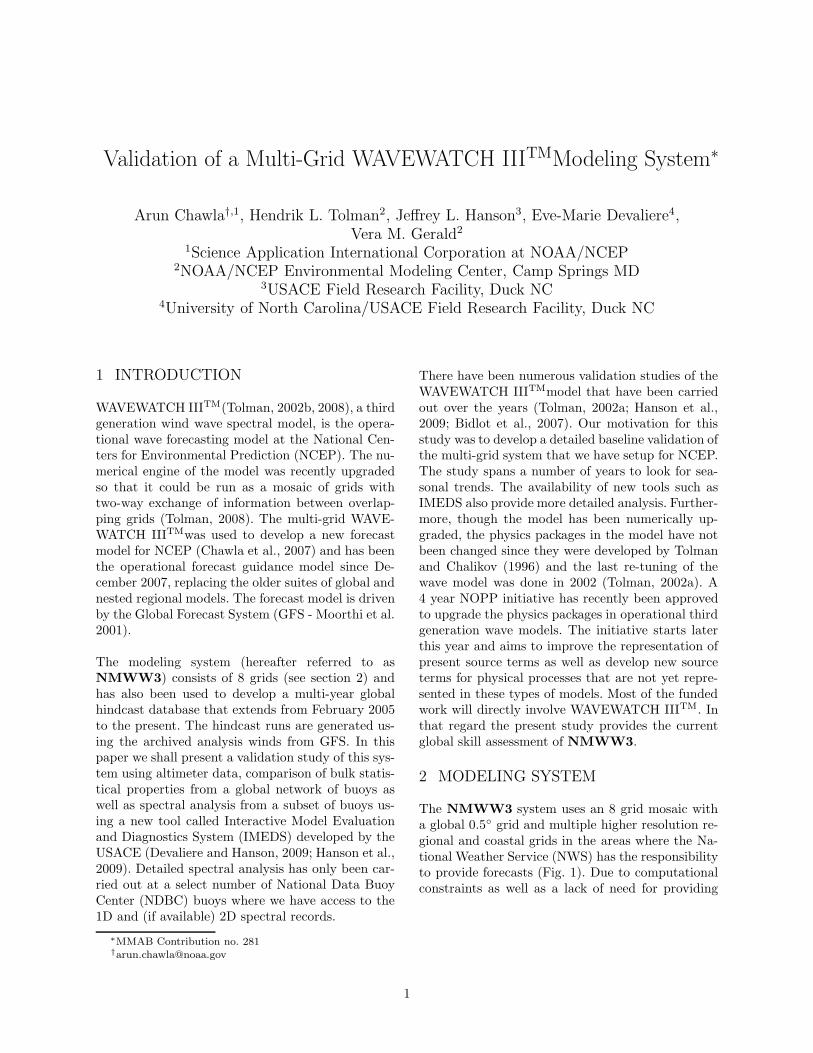
The NMWW3 system uses an 8 grid mosaic witha global 0.5◦ grid and multiple higher resolution re-gional and coastal grids in the areas where the Na-tional Weather Service (NWS) has the responsibilityto provide forecasts (Fig. 1). Due to computationalconstraints as well as a lack of need for providing

∗MMAB Contribution no. 281†[email protected]

1

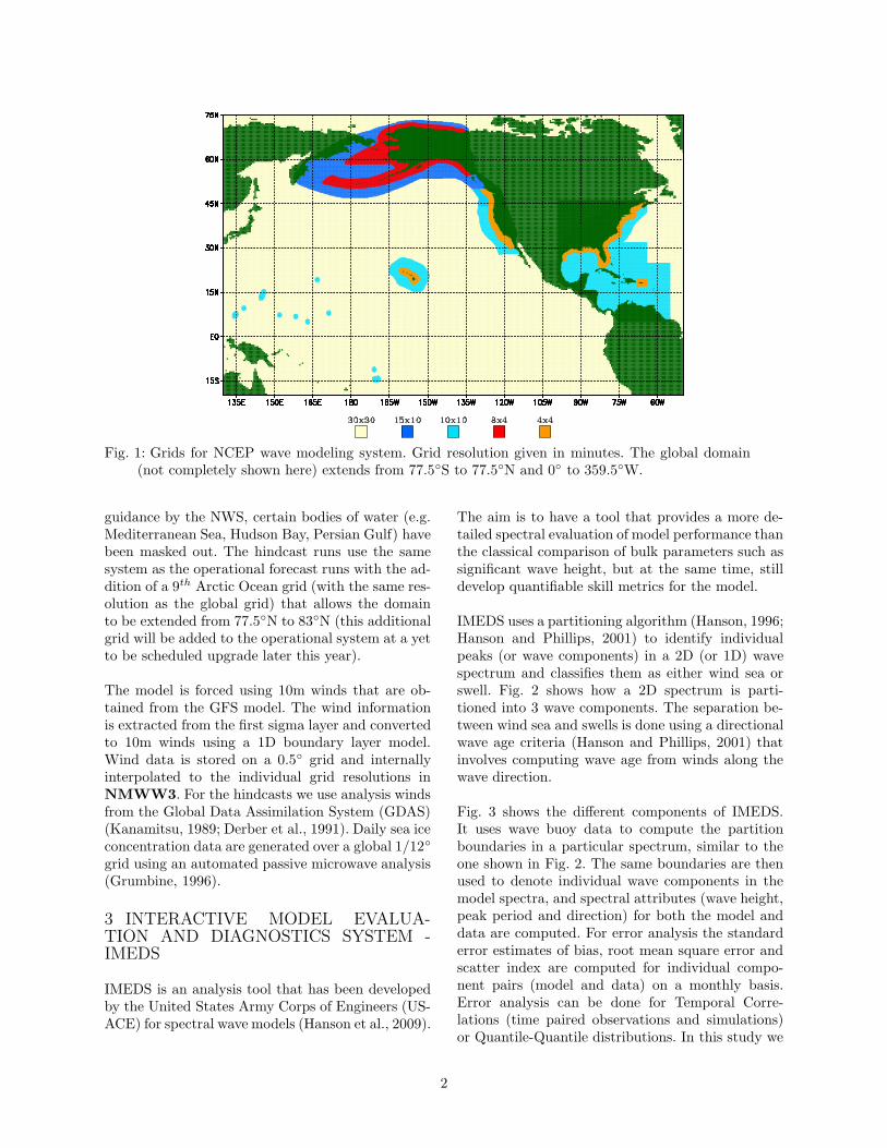
Fig. 1: Grids for NCEP wave modeling system. Grid resolution given in minutes. The global domain(not completely shown here) extends from 77.5◦S to 77.5◦N and 0◦ to 359.5◦W.

guidance by the NWS, certain bodies of water (e.g.Mediterranean Sea, Hudson Bay, Persian Gulf) havebeen masked out. The hindcast runs use the samesystem as the operational forecast runs with the ad-dition of a 9th Arctic Ocean grid (with the same res-olution as the global grid) that allows the domainto be extended from 77.5◦N to 83◦N (this additionalgrid will be added to the operational system at a yetto be scheduled upgrade later this year).

The model is forced using 10m winds that are ob-tained from the GFS model. The wind informationis extracted from the first sigma layer and convertedto 10m winds using a 1D boundary layer model.Wind data is stored on a 0.5◦ grid and internallyinterpolated to the individual grid resolutions inNMWW3. For the hindcasts we use analysis windsfrom the Global Data Assimilation System (GDAS)(Kanamitsu, 1989; Derber et al., 1991). Daily sea iceconcentration data are generated over a global 1/12◦

grid using an automated passive microwave analysis(Grumbine, 1996).

3 INTERACTIVE MODEL EVALUA-TION AND DIAGNOSTICS SYSTEM -IMEDS

IMEDS is an analysis tool that has been developedby the United States Army Corps of Engineers (US-ACE) for spectral wave models (Hanson et al., 2009).

The aim is to have a tool that provides a more de-tailed spectral evaluation of model performance thanthe classical comparison of bulk parameters such assignificant wave height, but at the same time, stilldevelop quantifiable skill metrics for the model.

IMEDS uses a partitioning algorithm (Hanson, 1996;Hanson and Phillips, 2001) to identify individualpeaks (or wave components) in a 2D (or 1D) wavespectrum and classifies them as either wind sea orswell. Fig. 2 shows how a 2D spectrum is parti-tioned into 3 wave components. The separation be-tween wind sea and swells is done using a directionalwave age criteria (Hanson and Phillips, 2001) thatinvolves computing wave age from winds along thewave direction.

Fig. 3 shows the different components of IMEDS.It uses wave buoy data to compute the partitionboundaries in a particular spectrum, similar to theone shown in Fig. 2. The same boundaries are thenused to denote individual wave components in themodel spectra, and spectral attributes (wave height,peak period and direction) for both the model anddata are computed. For error analysis the standarderror estimates of bias, root mean square error andscatter index are computed for individual compo-nent pairs (model and data) on a monthly basis.Error analysis can be done for Temporal Corre-lations (time paired observations and simulations)or Quantile-Quantile distributions. In this study we

2

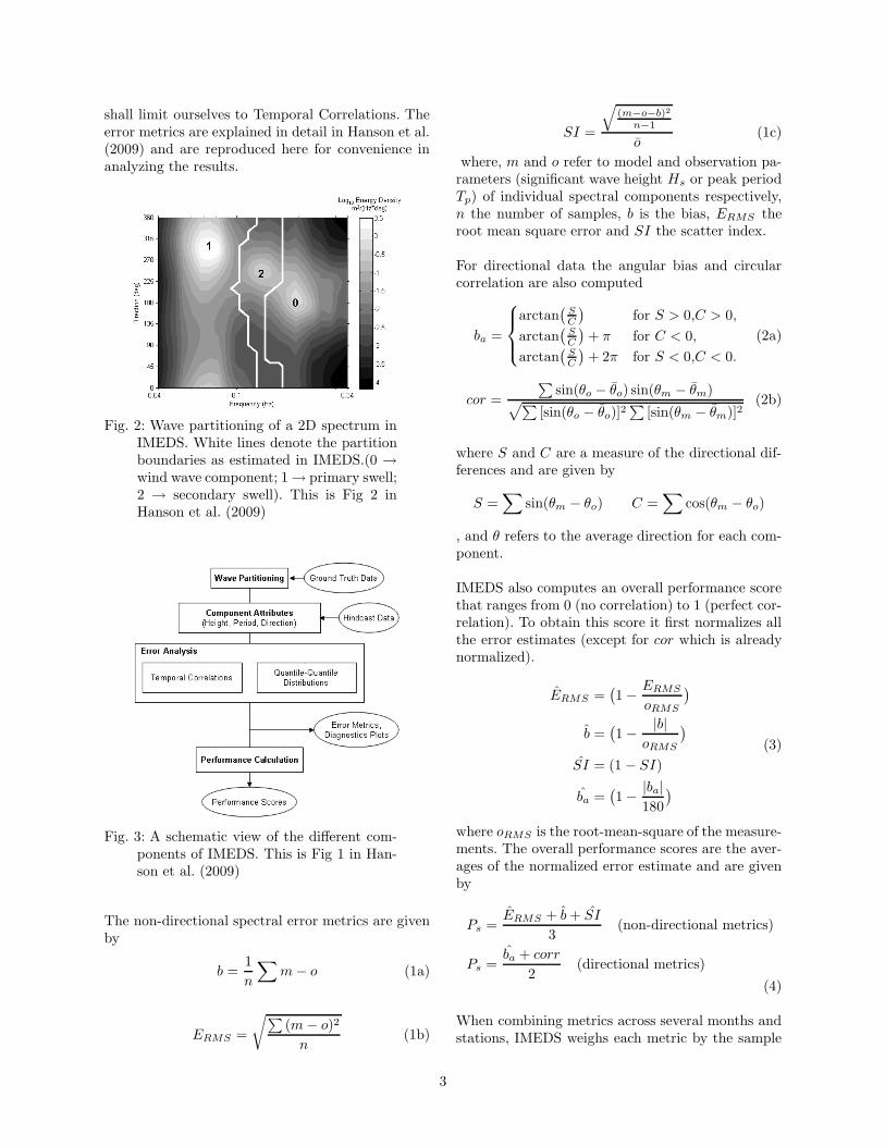
shall limit ourselves to Temporal Correlations. Theerror metrics are explained in detail in Hanson et al.(2009) and are reproduced here for convenience inanalyzing the results.

Fig. 2: Wave partitioning of a 2D spectrum inIMEDS. White lines denote the partitionboundaries as estimated in IMEDS.(0 →wind wave component; 1 → primary swell;2 → secondary swell). This is Fig 2 inHanson et al. (2009)

Fig. 3: A schematic view of the different com-ponents of IMEDS. This is Fig 1 in Han-son et al. (2009)

The non-directional spectral error metrics are givenby

b =1

n

∑

m − o (1a)

ERMS =

√

∑

(m − o)2

n(1b)

SI =

√

(m−o−b)2

n−1

o(1c)

where, m and o refer to model and observation pa-rameters (significant wave height Hs or peak periodTp) of individual spectral components respectively,n the number of samples, b is the bias, ERMS theroot mean square error and SI the scatter index.

For directional data the angular bias and circularcorrelation are also computed

ba =

arctan(

SC

)

for S > 0,C > 0,

arctan(

SC

)

+ π for C < 0,

arctan(

SC

)

+ 2π for S < 0,C < 0.

(2a)

cor =

∑

sin(θo − θo) sin(θm − θm)√

∑

[sin(θo − θo)]2∑

[sin(θm − θm)]2(2b)

where S and C are a measure of the directional dif-ferences and are given by

S =∑

sin(θm − θo) C =∑

cos(θm − θo)

, and θ refers to the average direction for each com-ponent.

IMEDS also computes an overall performance scorethat ranges from 0 (no correlation) to 1 (perfect cor-relation). To obtain this score it first normalizes allthe error estimates (except for cor which is alreadynormalized).

ERMS =(

1 −ERMS

oRMS

)

b =(

1 −|b|

oRMS

)

SI = (1 − SI)

ba =(

1 −|ba|

180

)

(3)

where oRMS is the root-mean-square of the measure-ments. The overall performance scores are the aver-ages of the normalized error estimate and are givenby

Ps =ERMS + b + SI

3(non-directional metrics)

Ps =ba + corr

2(directional metrics)

(4)

When combining metrics across several months andstations, IMEDS weighs each metric by the sample

3

size. We shall use this approach in this paper to ob-tain yearly skill scores for select NDBC buoys in theAtlantic and Pacific to compare the model perfor-mance in the two basins.

4 DATA ANALYSIS

Data analysis has been done using 3 different sourcesof data − altimeter data from the Jason-1 satellite toobtain spatial maps of error estimates, bulk spectralestimates from a global network of buoys to look atdetailed temporal patterns at different locations inthe world and spectral analysis using IMEDS to es-timate which part of the spectrum plays a dominantrole in the overall errors of the system.

4.a Altimeter comparisons

For altimeter comparisons we rely on the Jason-1satellite data to provide estimates of Hs. The al-timeter data used is the so called “fast delivery” datawhich is available in near real time. Since the model-ing system went into operations daily files of altime-ter and collocated model (for hindcast and severalforecast periods) are being generated and archived aspart of the operational suite of products. Error met-rics have been computed using month long recordsof this daily archive to ensure global coverage. Cal-ibration and validation of the fast delivery satellitedata with buoy measurements was done by Tolmanet al. (2006) and as part of this study were confirmedagain using the 2008 altimeter data set (figure notshown).

0 24 48 72 96 12010

15

20

25

30

35Jan08

0 24 48 72 96 12010

15

20

25

30

35Apr08

0 24 48 72 96 12010

15

20

25

30

35Jul08

0 24 48 72 96 12010

15

20

25

30

35Oct08

Raw 7 11 15

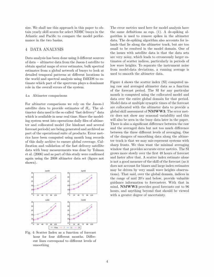
Fig. 4: Scatter Index as a function of forecasthour for four different months. Differ-ent lines correspond to different levels ofsmoothing

The error metrics used here for model analysis havethe same definitions as eqn. (1). A de-spiking al-gorithm is used to remove spikes in the altimeterdata. The de-spiking algorithm also accounts for is-lands that lie along the altimeter track, but are toosmall to be resolved in the model domain. One ofthe issues with satellite data is that the data setsare very noisy, which leads to erroneously larger es-timates of scatter indices, particularly in periods oflow wave heights. To separate the instrument noisefrom model-data deviations, a running average isused to smooth the altimeter data.

Figure 4 shows the scatter index (SI) computed us-ing raw and averaged altimeter data as a functionof the forecast period. The SI for any particularmonth is computed using the collocated model anddata over the entire global domain for that period.Model data at multiple synoptic times of the forecastare collocated with the altimeter data to provide aglobal skill assessment of NMWW3. The error met-ric does not show any seasonal variability and thiswill also be seen in the buoy data later in the paper.There is also a significant difference between the rawand the averaged data but not too much differencebetween the three different levels of averaging. Oneof the dangers of smoothing data along the altime-ter track is that we may mis-represent systems withsharp fronts. We thus want the minimal averagingwindow that provides accurate error metrics. The SIgrows more slowly over the first 48 hours of forecastand faster after that. A scatter index estimate aloneis not a good measure of the skill of the forecast (as itdoes not account for biases and large index estimatesmay be driven by very small wave heights observa-tions). That said, over the global domain, indices inthe range of mid 20’s and below, provide valuableguidance information to forecasters. With that inmind, NMWW3 provides good forecasts out to 96hours, and anything beyond that should be viewedwith a greater degree of uncertainty.

4

(a) Hindcast (b) 48 Hr Forecast

(c) 72 Hr Forecast (d) 96 Hr Forecast

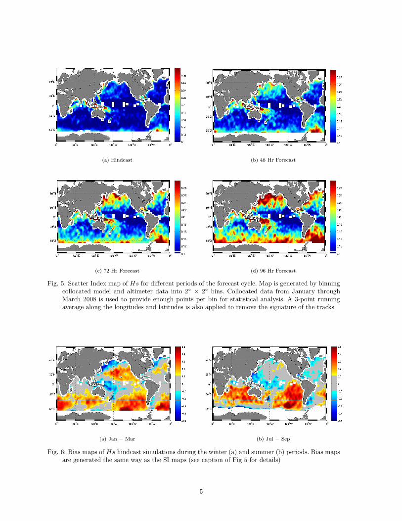
Fig. 5: Scatter Index map of Hs for different periods of the forecast cycle. Map is generated by binningcollocated model and altimeter data into 2◦ × 2◦ bins. Collocated data from January throughMarch 2008 is used to provide enough points per bin for statistical analysis. A 3-point runningaverage along the longitudes and latitudes is also applied to remove the signature of the tracks

(a) Jan − Mar (b) Jul − Sep

Fig. 6: Bias maps of Hs hindcast simulations during the winter (a) and summer (b) periods. Bias mapsare generated the same way as the SI maps (see caption of Fig 5 for details)

5

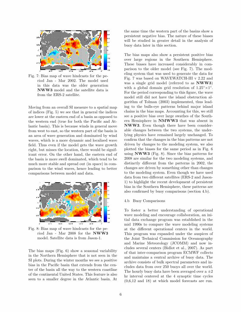
Fig. 7: Bias map of wave hindcasts for the pe-riod Jan - Mar 2002. The model usedin this data was the older generationNWW3 model and the satellite data isfrom the ERS-2 satellite.

Moving from an overall SI measure to a spatial mapof indices (Fig. 5) we see that in general the indicesare lower at the eastern end of a basin as opposed tothe western end (true for both the Pacific and At-lantic basin). This is because winds in general movefrom west to east, so the western part of the basin isan area of wave generation and dominated by windwaves, which is a more dynamic and localized wavefield. Thus even if the model gets the wave growthright, but misses the location, there would be signif-icant error. On the other hand, the eastern end ofthe basin is more swell dominated, which tend to bemuch more stable and spread out (in space) in com-parison to the wind waves, hence leading to bettercomparisons between model and data.

Fig. 8: Bias map of wave hindcasts for the pe-riod Jan - Mar 2008 for the NWW3

model. Satellite data is from Jason-1.

The bias maps (Fig. 6) show a seasonal variabilityin the Northern Hemisphere that is not seen in theSI plots. During the winter months we see a positivebias in the Pacific basin that extends from the cen-ter of the basin all the way to the western coastlineof the continental United States. This feature is alsoseen to a smaller degree in the Atlantic basin. At

the same time the western part of the basins show apersistent negative bias. The nature of these biaseswill be studied in greater detail in the analysis ofbuoy data later in this section.

The bias maps also show a persistent positive biasover large regions in the Southern Hemisphere.These biases have increased considerably in com-parison to the older model (see Fig. 7). The mod-eling system that was used to generate the data forFig. 7 was based on WAVEWATCH-III v 2.22 andwas a single grid model (referred to as NWW3)with a global domain grid resolution of 1.25◦×1◦.For the period corresponding to this figure, the wavemodel still did not have the island obstruction al-gorithm of Tolman (2003) implemented, thus lead-ing to the bulls-eye patterns behind major islandchains in the bias maps. Accounting for this, we stillsee a positive bias over large swathes of the South-ern Hemisphere in NMWW3 that was absent inNWW3. Even though there have been consider-able changes between the two systems, the under-lying physics have remained largely unchanged. Toconfirm that the changes in the bias patterns are notdriven by changes to the modeling system, we alsoplotted the biases for the same period as in Fig. 6using NWW3 (Fig. 8). Since the bias patterns for2008 are similar for the two modeling systems, anddistinctly different from the patterns in 2002, thechanges are driven by something other than changesto the modeling system. Even though we have useddata from two different satellites (ERS-2 and Jason-1) to highlight the recent development of persistentbias in the Southern Hemisphere, these patterns arealso confirmed by buoy comparisons (section 4.b).

4.b Buoy Comparisons

To foster a better understanding of operationalwave modeling and encourage collaboration, an ini-tial data exchange program was established in themid 1990s to compare the wave modeling systemsat the different operational centers in the world.This program was expanded under the auspices ofthe Joint Technical Commission for Oceanographyand Marine Meteorology (JCOMM) and now in-cludes several centers (Bidlot et al., 2007). As partof that inter-comparison program ECMWF collectsand maintains a central archive of buoy data. Thearchive consists of bulk spectral parameters and in-cludes data from over 250 buoys all over the world.The hourly buoy data have been averaged over a ±2hr interval centered at the 4 synoptic time cycles(0,6,12 and 18) at which model forecasts are run.

6

Longitude

Latit

ude

−180E −135E −90E −45E 0E 45E 90E 135E 180

45S

0

45N

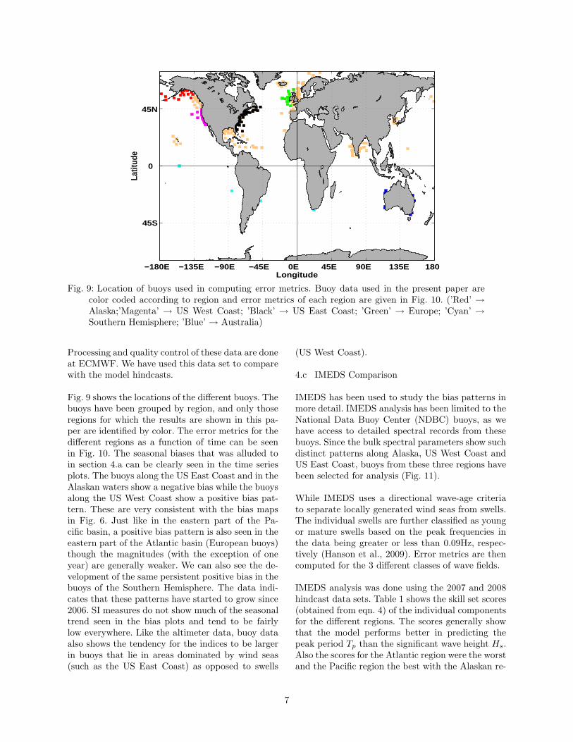
Fig. 9: Location of buoys used in computing error metrics. Buoy data used in the present paper arecolor coded according to region and error metrics of each region are given in Fig. 10. (’Red’ →Alaska;’Magenta’ → US West Coast; ’Black’ → US East Coast; ’Green’ → Europe; ’Cyan’ →Southern Hemisphere; ’Blue’ → Australia)

Processing and quality control of these data are doneat ECMWF. We have used this data set to comparewith the model hindcasts.

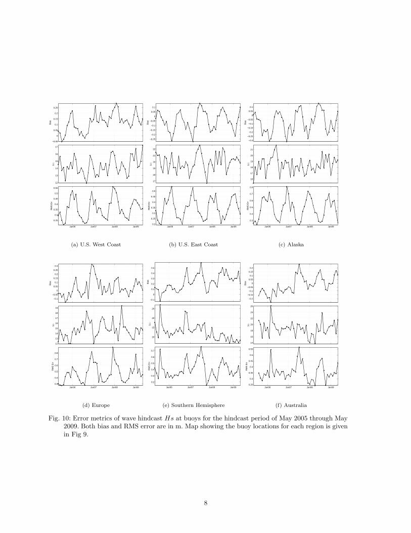
Fig. 9 shows the locations of the different buoys. Thebuoys have been grouped by region, and only thoseregions for which the results are shown in this pa-per are identified by color. The error metrics for thedifferent regions as a function of time can be seenin Fig. 10. The seasonal biases that was alluded toin section 4.a can be clearly seen in the time seriesplots. The buoys along the US East Coast and in theAlaskan waters show a negative bias while the buoysalong the US West Coast show a positive bias pat-tern. These are very consistent with the bias mapsin Fig. 6. Just like in the eastern part of the Pa-cific basin, a positive bias pattern is also seen in theeastern part of the Atlantic basin (European buoys)though the magnitudes (with the exception of oneyear) are generally weaker. We can also see the de-velopment of the same persistent positive bias in thebuoys of the Southern Hemisphere. The data indi-cates that these patterns have started to grow since2006. SI measures do not show much of the seasonaltrend seen in the bias plots and tend to be fairlylow everywhere. Like the altimeter data, buoy dataalso shows the tendency for the indices to be largerin buoys that lie in areas dominated by wind seas(such as the US East Coast) as opposed to swells

(US West Coast).

4.c IMEDS Comparison

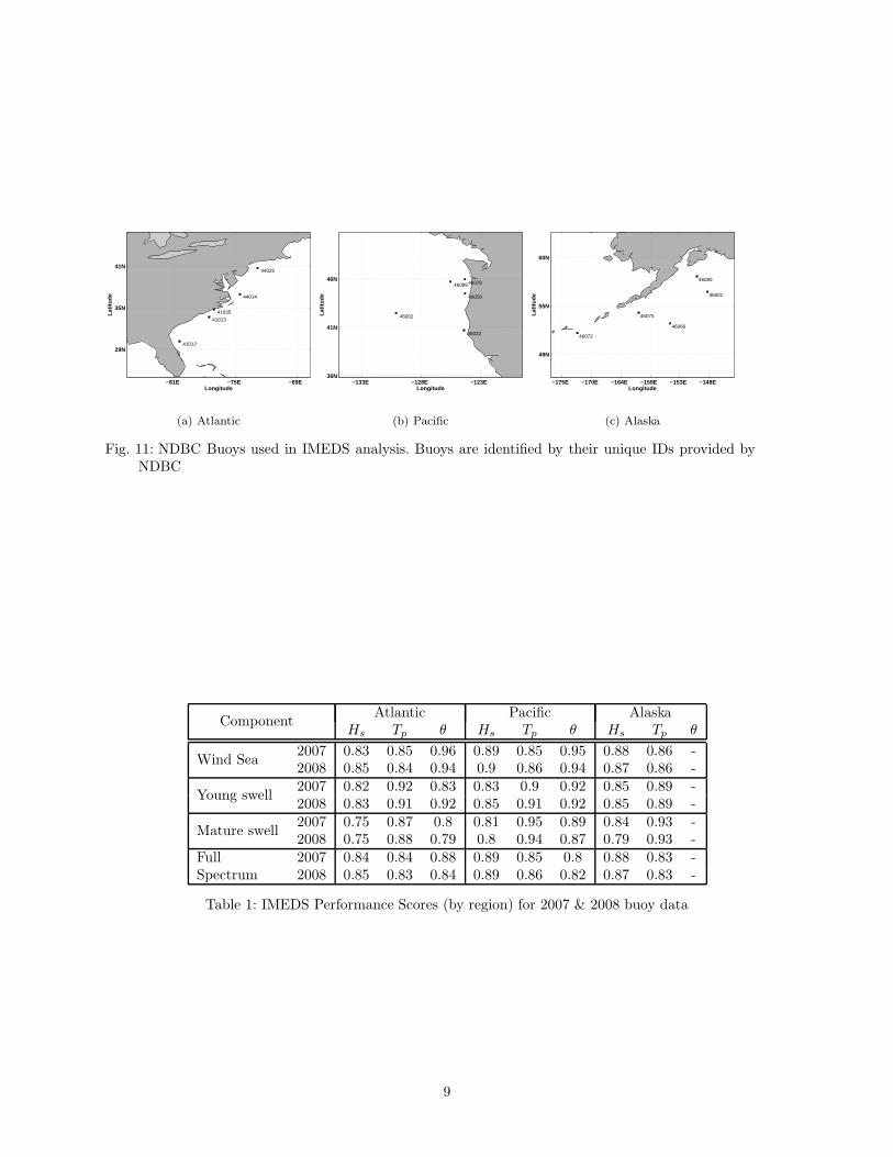
IMEDS has been used to study the bias patterns inmore detail. IMEDS analysis has been limited to theNational Data Buoy Center (NDBC) buoys, as wehave access to detailed spectral records from thesebuoys. Since the bulk spectral parameters show suchdistinct patterns along Alaska, US West Coast andUS East Coast, buoys from these three regions havebeen selected for analysis (Fig. 11).

While IMEDS uses a directional wave-age criteriato separate locally generated wind seas from swells.The individual swells are further classified as youngor mature swells based on the peak frequencies inthe data being greater or less than 0.09Hz, respec-tively (Hanson et al., 2009). Error metrics are thencomputed for the 3 different classes of wave fields.

IMEDS analysis was done using the 2007 and 2008hindcast data sets. Table 1 shows the skill set scores(obtained from eqn. 4) of the individual componentsfor the different regions. The scores generally showthat the model performs better in predicting thepeak period Tp than the significant wave height Hs.Also the scores for the Atlantic region were the worstand the Pacific region the best with the Alaskan re-

7

−0.05

0

0.05

0.1

0.15

0.2

0.25

Bia

s

12

13

14

15

16

17

S.I.

Jan06 Jan07 Jan08 Jan09

0.25

0.3

0.35

0.4

0.45

0.5

0.55

RM

S E

rr

(a) U.S. West Coast

−0.25

−0.2

−0.15

−0.1

−0.05

0

0.05

0.1

Bia

s

17

18

19

20

21

22S

.I.

Jan06 Jan07 Jan08 Jan090.2

0.25

0.3

0.35

0.4

0.45

0.5

RM

S E

rr

(b) U.S. East Coast

−0.3

−0.25

−0.2

−0.15

−0.1

−0.05

0

0.05

0.1

Bia

s

16

17

18

19

20

21

S.I.


0.3

0.4

0.5

0.6

0.7

0.8

RM

S E

rr(c) Alaska

−0.1

−0.05

0

0.05

0.1

0.15

0.2

0.25

0.3

Bia

s

12

13

14

15

16

17

18

19

S.I.


0.3

0.4

0.5

0.6

0.7

0.8

RM

S E

rr

(d) Europe

−0.1

0

0.1

0.2

0.3

0.4

0.5

Bia

s

10

15

20

25

S.I.


0.2

0.3

0.4

0.5

0.6

0.7

RM

S E

rr

(e) Southern Hemisphere

−0.2

−0.15

−0.1

−0.05

0

0.05

0.1

0.15

0.2

Bia

s

14

16

18

20

22

24

26

S.I.

Jan06 Jan07 Jan08 Jan090.25

0.3

0.35

0.4

0.45

0.5

0.55

RM

S E

rr

(f) Australia

Fig. 10: Error metrics of wave hindcast Hs at buoys for the hindcast period of May 2005 through May2009. Both bias and RMS error are in m. Map showing the buoy locations for each region is givenin Fig 9.

8

Longitude

Lat

itu

de

41012

41013

41035

44014

44025

−81E −75E −69E

29N

35N

41N

(a) Atlantic

Longitude

Lat

itu

de

46002

46022

46029

46050

46089

−133E −128E −123E36N

41N

46N

(b) Pacific

Longitude

Lat

itu

de 46001

46066

46072

46075

46080

−175E −170E −164E −159E −153E −148E

49N

55N

60N

(c) Alaska

Fig. 11: NDBC Buoys used in IMEDS analysis. Buoys are identified by their unique IDs provided byNDBC

ComponentAtlantic Pacific Alaska

Hs Tp θ Hs Tp θ Hs Tp θ

Wind Sea2007 0.83 0.85 0.96 0.89 0.85 0.95 0.88 0.86 -2008 0.85 0.84 0.94 0.9 0.86 0.94 0.87 0.86 -

Young swell2007 0.82 0.92 0.83 0.83 0.9 0.92 0.85 0.89 -2008 0.83 0.91 0.92 0.85 0.91 0.92 0.85 0.89 -

Mature swell2007 0.75 0.87 0.8 0.81 0.95 0.89 0.84 0.93 -2008 0.75 0.88 0.79 0.8 0.94 0.87 0.79 0.93 -

FullSpectrum

2007 0.84 0.84 0.88 0.89 0.85 0.8 0.88 0.83 -2008 0.85 0.83 0.84 0.89 0.86 0.82 0.87 0.83 -

Table 1: IMEDS Performance Scores (by region) for 2007 & 2008 buoy data

9

gion being in between. This is similar to what weobserved from the altimeter and bulk spectral pa-rameter comparisons at the buoys. The scores acrossthe two years are fairly similar and thus, for brevityonly the plots from the 2008 data sets are shownhere.

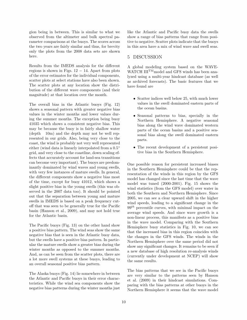
Results from the IMEDS analysis for the differentregions is shown in Figs. 12 − 14. Apart from plotsof the error estimates for the individual components,scatter plots at select stations have also been shown.The scatter plots at any location show the distri-bution of the different wave components (and theirmagnitude) at that location over the month.

The overall bias in the Atlantic buoys (Fig. 12)shows a seasonal pattern with greater negative biasvalues in the winter months and lower values dur-ing the summer months. The exception being buoy41035 which shows a consistent negative bias. Thismay be because the buoy is in fairly shallow water(depth 10m) and the depth may not be well rep-resented in our grids. Also, being very close to thecoast, the wind is probably not very well representedeither (wind data is linearly interpolated from a 0.5◦

grid, and very close to the coastline, down scaling ef-fects that accurately account for land-sea transitionscan become very important). The buoys are predom-inantly dominated by wind waves and young swells,with very few instances of mature swells. In general,the different components show a negative bias mostof the time, except for buoy 41012, which shows aslight positive bias in the young swells (this was ob-served in the 2007 data too). It should be pointedout that the separation between young and matureswells in IMEDS is based on a peak frequency cut-off that was seen to be generally true for the Pacificbasin (Hanson et al., 2009), and may not hold truefor the Atlantic basin.

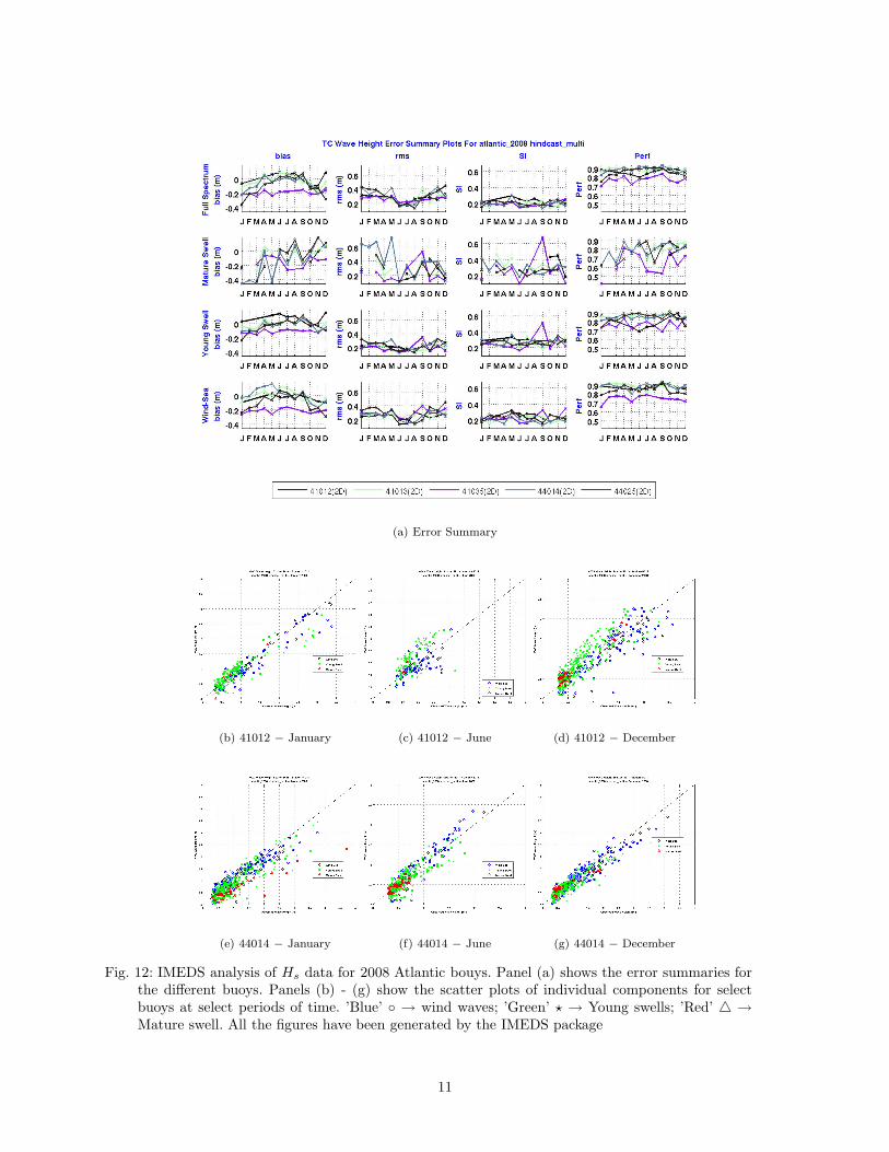
The Pacific buoys (Fig. 13) on the other hand showa positive bias pattern. The wind seas show the samenegative bias that is seen in the Atlantic buoy data,but the swells have a positive bias pattern. In partic-ular the mature swells show a greater bias during thewinter months as opposed to the summer months.And, as can be seen from the scatter plots, there area lot more swell systems at these buoys, leading toan overall seasonal positive bias pattern.

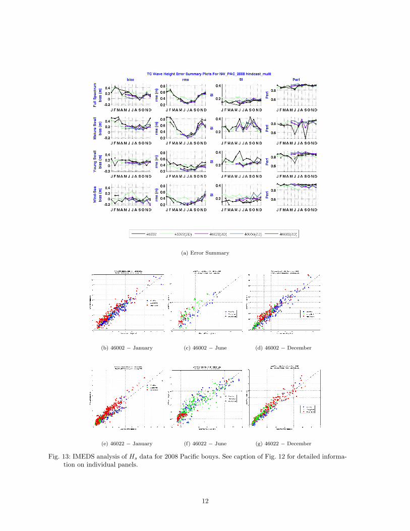
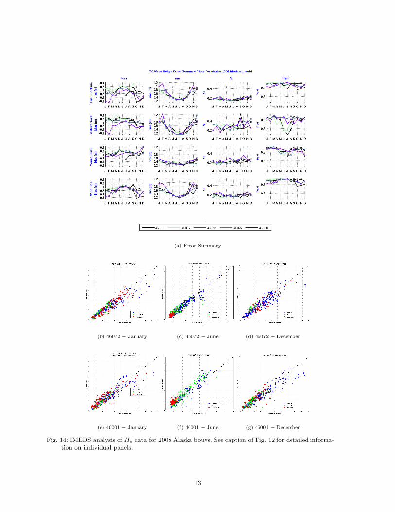
The Alaska buoys (Fig. 14) lie somewhere in betweenthe Atlantic and Pacific buoys in their error charac-teristics. While the wind sea components show thenegative bias patterns during the winter months just

like the Atlantic and Pacific buoy data the swellsshow a range of bias patterns that range from posi-tive to negative. Scatter plots indicate that the buoysin this area have a mix of wind wave and swell seas.

5 DISCUSSION

A global modeling system based on the WAVE-WATCH IIITMmodel and GFS winds has been ana-lyzed using a multi-year hindcast database (as wellas archived forecasts). The basic features that wehave found are

• Scatter indices well below 25, with much lowervalues in the swell dominated eastern parts ofthe ocean basins.

• Seasonal patterns to bias, specially in theNorthern Hemisphere. A negative seasonalbias along the wind wave dominated westernparts of the ocean basins and a positive sea-sonal bias along the swell dominated easternparts.

• The recent development of a persistent posi-tive bias in the Southern Hemisphere.

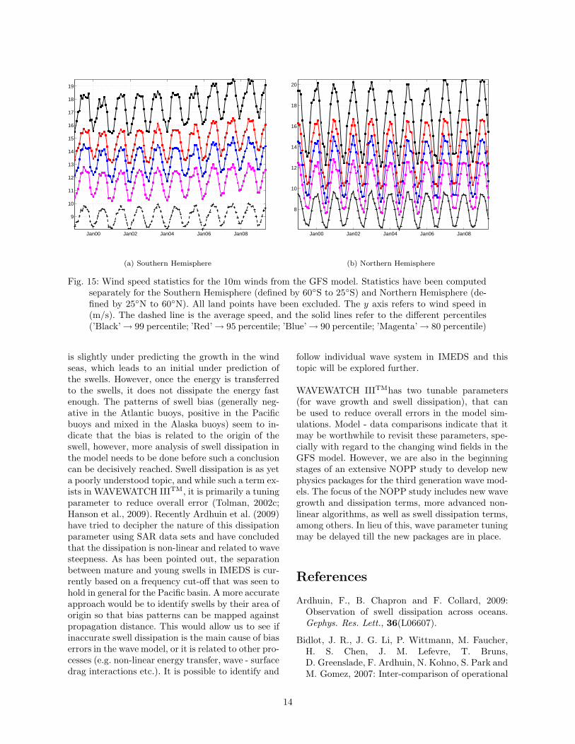
One possible reason for persistent increased biasesin the Southern Hemisphere could be that the rep-resentation of the winds in this region by the GFSmodel has changed since the last time that the wavemodel was tuned (2000-2001). Fig. 15 shows thewind statistics (from the GFS model) over water inboth the Southern and Northern Hemisphere. Since2005, we can see a clear upward shift in the higherwind speeds, leading to a significant change in the99th percentile curves, with minimal impact on theaverage wind speeds. And since wave growth is anon-linear process, this manifests as a positive biasin the wave model. Comparing with the SouthernHemisphere buoy statistics in Fig. 10, we can seethat the increased bias in this region coincides withthe changes in the GFS winds. The winds in theNorthern Hemisphere over the same period did notshow any significant changes. It remains to be seen ifa new database of high resolution re-analysis winds(currently under development at NCEP) will showthe same results.

The bias patterns that we see in the Pacific buoysare very similar to the patterns seen by Hansonet al. (2009) in their hindcast simulations. Com-paring with the bias patterns at other buoys in theNorthern Hemisphere it seems that the wave model

10

(a) Error Summary

(b) 41012 − January (c) 41012 − June (d) 41012 − December

(e) 44014 − January (f) 44014 − June (g) 44014 − December

Fig. 12: IMEDS analysis of Hs data for 2008 Atlantic bouys. Panel (a) shows the error summaries forthe different buoys. Panels (b) - (g) show the scatter plots of individual components for selectbuoys at select periods of time. ’Blue’ ◦ → wind waves; ’Green’ ? → Young swells; ’Red’ 4 →Mature swell. All the figures have been generated by the IMEDS package

11

(a) Error Summary



Fig. 13: IMEDS analysis of Hs data for 2008 Pacific bouys. See caption of Fig. 12 for detailed informa-tion on individual panels.

12

(a) Error Summary



Fig. 14: IMEDS analysis of Hs data for 2008 Alaska bouys. See caption of Fig. 12 for detailed informa-tion on individual panels.

13

Jan00 Jan02 Jan04 Jan06 Jan08

9

10

11

12

13

14

15

16

17

18

19

(a) Southern Hemisphere

Jan00 Jan02 Jan04 Jan06 Jan08

8

10

12

14

16

18

20

(b) Northern Hemisphere

Fig. 15: Wind speed statistics for the 10m winds from the GFS model. Statistics have been computedseparately for the Southern Hemisphere (defined by 60◦S to 25◦S) and Northern Hemisphere (de-fined by 25◦N to 60◦N). All land points have been excluded. The y axis refers to wind speed in(m/s). The dashed line is the average speed, and the solid lines refer to the different percentiles(’Black’ → 99 percentile; ’Red’ → 95 percentile; ’Blue’ → 90 percentile; ’Magenta’ → 80 percentile)

is slightly under predicting the growth in the windseas, which leads to an initial under prediction ofthe swells. However, once the energy is transferredto the swells, it does not dissipate the energy fastenough. The patterns of swell bias (generally neg-ative in the Atlantic buoys, positive in the Pacificbuoys and mixed in the Alaska buoys) seem to in-dicate that the bias is related to the origin of theswell, however, more analysis of swell dissipation inthe model needs to be done before such a conclusioncan be decisively reached. Swell dissipation is as yeta poorly understood topic, and while such a term ex-ists in WAVEWATCH IIITM, it is primarily a tuningparameter to reduce overall error (Tolman, 2002c;Hanson et al., 2009). Recently Ardhuin et al. (2009)have tried to decipher the nature of this dissipationparameter using SAR data sets and have concludedthat the dissipation is non-linear and related to wavesteepness. As has been pointed out, the separationbetween mature and young swells in IMEDS is cur-rently based on a frequency cut-off that was seen tohold in general for the Pacific basin. A more accurateapproach would be to identify swells by their area oforigin so that bias patterns can be mapped againstpropagation distance. This would allow us to see ifinaccurate swell dissipation is the main cause of biaserrors in the wave model, or it is related to other pro-cesses (e.g. non-linear energy transfer, wave - surfacedrag interactions etc.). It is possible to identify and

follow individual wave system in IMEDS and thistopic will be explored further.

WAVEWATCH IIITMhas two tunable parameters(for wave growth and swell dissipation), that canbe used to reduce overall errors in the model sim-ulations. Model - data comparisons indicate that itmay be worthwhile to revisit these parameters, spe-cially with regard to the changing wind fields in theGFS model. However, we are also in the beginningstages of an extensive NOPP study to develop newphysics packages for the third generation wave mod-els. The focus of the NOPP study includes new wavegrowth and dissipation terms, more advanced non-linear algorithms, as well as swell dissipation terms,among others. In lieu of this, wave parameter tuningmay be delayed till the new packages are in place.

References

Ardhuin, F., B. Chapron and F. Collard, 2009:Observation of swell dissipation across oceans.Gephys. Res. Lett., 36(L06607).

Bidlot, J. R., J. G. Li, P. Wittmann, M. Faucher,H. S. Chen, J. M. Lefevre, T. Bruns,D. Greenslade, F. Ardhuin, N. Kohno, S. Park andM. Gomez, 2007: Inter-comparison of operational

14

wave forecasting systems. in 10th International

workshop on wave hindcasting and forecasting,Oahu, Hawaii.

Chawla, A., D. Cao, V. Gerald, T. Spindler andH. Tolman, 2007: Operational implementation of amulti-grid wave forecasting system. in 10th Inter-

national workshop on wave hindcasting and fore-

casting, p. pp 12, Oahu, Hawaii.

Derber, J. C., D. F. Parrish and S. J. Lord, 1991: Thenew global operational analysis system at the Na-tional Meteorological Center. Weather and Fore-

casting, 6, 538–547.

Devaliere, E.-M. and J. Hanson, 2009: IMEDS Inter-

active Model Evaluation and Diagnostics System

V2.6 Users Guide. US Army Corps of Engineers,Field Research Facility, Duck, NC.

Grumbine, R. W., 1996: Automated passive mi-crowave sea ice concentration analysis. Technicalnote 120, NCEP/NOAA/NWS, National Centerfor Environmental Prediction, Washington DC.

Hanson, J. L., 1996: Wind sea growth and swell evo-

lution in the Gulf of Alaska. Ph.D. thesis, JohnsHopkins University.

Hanson, J. L. and O. M. Phillips, 2001: Automatedanalysis of ocean surface directional wave spectra.J. Atmos. Oceanic Technol., 18, 277 – 293.

Hanson, J. L., B. A. Tracy, H. L. Tolman and R. D.Scott, 2009: Pacific hindcast performance of threenumerical wave models. Journal of Atmospheric

and Oceanic Technology, 26, 1614 – 1633.

Kanamitsu, M., 1989: Description of the NMC globaldata assimilation and forecast system. Weather

and Forecasting, 4, 335–342.

Moorthi, S., H.-L. Pan and P. Caplan, 2001: Changesto the 2001 ncep Operational MRF/AVN GlobalAnalysis/Forecast System. Technical ProceduresBulletin 484, NWS/NCEP.

Tolman, H. L., 2002a: Testing of WAVEWATCH IIIversion 2.22 in NCEP’s NWW3 ocean wave modelsuite. Technical note 214, NCEP/NOAA/NWS,National Center for Environmental Prediction,Washington DC.

Tolman, H. L., 2002b: User manual and sys-tem documentation of WAVEWATCH III version2.22. Technical note 222, NCEP/NOAA/NWS,National Center for Environmental Prediction,Washington DC.

Tolman, H. L., 2002c: Validation of WAVEWATCHIII version 1.15 for a global domain. Technicalnote 213, NCEP/NOAA/NWS, National Centerfor Environmental Prediction, Washington DC.

Tolman, H. L., 2003: Treatment of unresolved islandsand ice in wind wave models. Ocean Modelling, 5,219 – 231.

Tolman, H. L., 2008: A mosaic approach to windwave modeling. Ocean Modelling, 25, 35–47.

Tolman, H. L., D. Cao and V. M. Gerald, 2006: Al-timeter data for use in wave models at ncep. Tech.Rep. 252, NCEP/NOAA/NWS, National Centerfor Environmental Prediction, Wasjington DC.

Tolman, H. L. and D. Chalikov, 1996: Source termsin a thrid generation wind wave model. Journal of

Physical Oceanography, 26, 2497–2518.

15

Documents

Validation of a Multi-Grid WAVEWATCH III Modeling System