Corrosion Science 52 (2010) 3514–3522

Contents lists available at ScienceDirect

Corrosion Science

journal homepage: www.elsevier .com/locate /corsc i

Validated numerical modelling of galvanic corrosion for couples: Magnesiumalloy (AE44)–mild steel and AE44–aluminium alloy (AA6063) in brine solution

Kiran B. Deshpande *

General Motors R&D, India Science Lab, Creator Building, ITPL, Bangalore 560066, India

a r t i c l e i n f o

Article history:Received 6 April 2010Accepted 30 June 2010Available online 8 July 2010

Keywords:A. MagnesiumA. AluminiumA. Mild steelB. Modelling studiesC. Corrosion

0010-938X/$ - see front matter � 2010 Elsevier Ltd. Adoi:10.1016/j.corsci.2010.06.031

* Tel.: +91 8041984560; fax: +91 8041158562.E-mail address: kiran.deshpande@gm.com

a b s t r a c t

A numerical model is presented in this work that predicts the corrosion rate of a galvanic couple. Themodel is capable of tracking moving boundary of the corroding constituent of the couple. The corrosionrates obtained from the model are compared with those estimated from mixed potential theory and twoexperimental techniques, namely Scanning Vibrating Electrode Technique (SVET) and immersion tech-nique. The corrosion rates predicted using the model are in good agreement with those estimated fromthe experimental techniques for magnesium alloy AE44–mild steel couple, however, the model underpredicts the corrosion rate for AE44–aluminium alloy AA6063 couple.

� 2010 Elsevier Ltd. All rights reserved.

1. Introduction

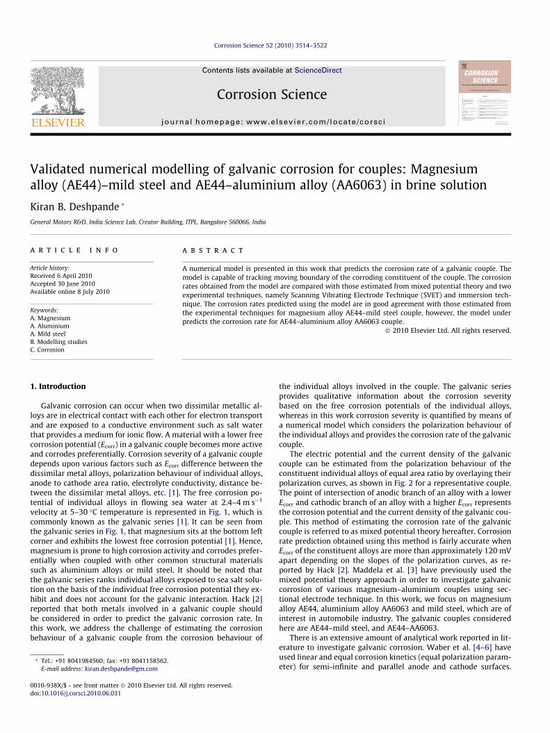
Galvanic corrosion can occur when two dissimilar metallic al-loys are in electrical contact with each other for electron transportand are exposed to a conductive environment such as salt waterthat provides a medium for ionic flow. A material with a lower freecorrosion potential (Ecorr) in a galvanic couple becomes more activeand corrodes preferentially. Corrosion severity of a galvanic coupledepends upon various factors such as Ecorr difference between thedissimilar metal alloys, polarization behaviour of individual alloys,anode to cathode area ratio, electrolyte conductivity, distance be-tween the dissimilar metal alloys, etc. [1]. The free corrosion po-tential of individual alloys in flowing sea water at 2.4–4 m s�1

velocity at 5–30 �C temperature is represented in Fig. 1, which iscommonly known as the galvanic series [1]. It can be seen fromthe galvanic series in Fig. 1, that magnesium sits at the bottom leftcorner and exhibits the lowest free corrosion potential [1]. Hence,magnesium is prone to high corrosion activity and corrodes prefer-entially when coupled with other common structural materialssuch as aluminium alloys or mild steel. It should be noted thatthe galvanic series ranks individual alloys exposed to sea salt solu-tion on the basis of the individual free corrosion potential they ex-hibit and does not account for the galvanic interaction. Hack [2]reported that both metals involved in a galvanic couple shouldbe considered in order to predict the galvanic corrosion rate. Inthis work, we address the challenge of estimating the corrosionbehaviour of a galvanic couple from the corrosion behaviour of

ll rights reserved.

the individual alloys involved in the couple. The galvanic seriesprovides qualitative information about the corrosion severitybased on the free corrosion potentials of the individual alloys,whereas in this work corrosion severity is quantified by means ofa numerical model which considers the polarization behaviour ofthe individual alloys and provides the corrosion rate of the galvaniccouple.

The electric potential and the current density of the galvaniccouple can be estimated from the polarization behaviour of theconstituent individual alloys of equal area ratio by overlaying theirpolarization curves, as shown in Fig. 2 for a representative couple.The point of intersection of anodic branch of an alloy with a lowerEcorr and cathodic branch of an alloy with a higher Ecorr representsthe corrosion potential and the current density of the galvanic cou-ple. This method of estimating the corrosion rate of the galvaniccouple is referred to as mixed potential theory hereafter. Corrosionrate prediction obtained using this method is fairly accurate whenEcorr of the constituent alloys are more than approximately 120 mVapart depending on the slopes of the polarization curves, as re-ported by Hack [2]. Maddela et al. [3] have previously used themixed potential theory approach in order to investigate galvaniccorrosion of various magnesium–aluminium couples using sec-tional electrode technique. In this work, we focus on magnesiumalloy AE44, aluminium alloy AA6063 and mild steel, which are ofinterest in automobile industry. The galvanic couples consideredhere are AE44–mild steel, and AE44–AA6063.

There is an extensive amount of analytical work reported in lit-erature to investigate galvanic corrosion. Waber et al. [4–6] haveused linear and equal corrosion kinetics (equal polarization param-eter) for semi-infinite and parallel anode and cathode surfaces.

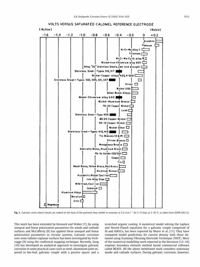
Fig. 1. Galvanic series where metals are ranked on the basis of the potential they exhibit in seawater at 2.4–4 m s�1 for 5–15 days at 5–30 �C, as taken from ASTM G82 [1].

K.B. Deshpande / Corrosion Science 52 (2010) 3514–3522 3515

This work has been extended by Kennard and Waber [7], by usingunequal and linear polarization parameters for anode and cathodesurfaces and McCafferty [8] has applied these unequal and linearpolarization parameters to circular systems. Galvanic corrosionover semi-infinite coplanar surfaces has been investigated by Verb-rugge [9] using the conformal mapping technique. Recently, Song[10] has developed an analytical approach to investigate galvaniccorrosion in some practical cases such as steel–aluminium joint ex-posed to bio-fuel, galvanic couple with a passive spacer and a

scratched organic coating. A numerical model solving the Laplaceand Nernst-Planck equations for a galvanic couple comprised ofAl and Al4%Cu, has been reported by Murer et al. [11]. They havecompared model predictions for current density with those ob-tained using Scanning Vibrating Electrode Technique (SVET). Mostof the numerical modelling work reported in the literature [12–16]employs boundary element method based commercial softwarecalled BEASY. All the above mentioned work considers stationaryanode and cathode surfaces. During galvanic corrosion, however,

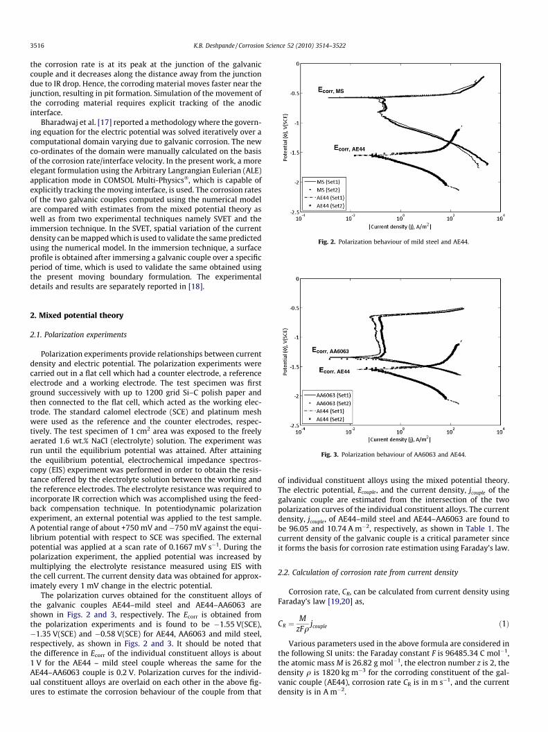
Fig. 2. Polarization behaviour of mild steel and AE44.

3516 K.B. Deshpande / Corrosion Science 52 (2010) 3514–3522

the corrosion rate is at its peak at the junction of the galvaniccouple and it decreases along the distance away from the junctiondue to IR drop. Hence, the corroding material moves faster near thejunction, resulting in pit formation. Simulation of the movement ofthe corroding material requires explicit tracking of the anodicinterface.

Bharadwaj et al. [17] reported a methodology where the govern-ing equation for the electric potential was solved iteratively over acomputational domain varying due to galvanic corrosion. The newco-ordinates of the domain were manually calculated on the basisof the corrosion rate/interface velocity. In the present work, a moreelegant formulation using the Arbitrary Langrangian Eulerian (ALE)application mode in COMSOL Multi-Physics�, which is capable ofexplicitly tracking the moving interface, is used. The corrosion ratesof the two galvanic couples computed using the numerical modelare compared with estimates from the mixed potential theory aswell as from two experimental techniques namely SVET and theimmersion technique. In the SVET, spatial variation of the currentdensity can be mapped which is used to validate the same predictedusing the numerical model. In the immersion technique, a surfaceprofile is obtained after immersing a galvanic couple over a specificperiod of time, which is used to validate the same obtained usingthe present moving boundary formulation. The experimentaldetails and results are separately reported in [18].

Fig. 3. Polarization behaviour of AA6063 and AE44.

2. Mixed potential theory

2.1. Polarization experiments

Polarization experiments provide relationships between currentdensity and electric potential. The polarization experiments werecarried out in a flat cell which had a counter electrode, a referenceelectrode and a working electrode. The test specimen was firstground successively with up to 1200 grid Si–C polish paper andthen connected to the flat cell, which acted as the working elec-trode. The standard calomel electrode (SCE) and platinum meshwere used as the reference and the counter electrodes, respec-tively. The test specimen of 1 cm2 area was exposed to the freelyaerated 1.6 wt.% NaCl (electrolyte) solution. The experiment wasrun until the equilibrium potential was attained. After attainingthe equilibrium potential, electrochemical impedance spectros-copy (EIS) experiment was performed in order to obtain the resis-tance offered by the electrolyte solution between the working andthe reference electrodes. The electrolyte resistance was required toincorporate IR correction which was accomplished using the feed-back compensation technique. In potentiodynamic polarizationexperiment, an external potential was applied to the test sample.A potential range of about +750 mV and�750 mV against the equi-librium potential with respect to SCE was specified. The externalpotential was applied at a scan rate of 0.1667 mV s�1. During thepolarization experiment, the applied potential was increased bymultiplying the electrolyte resistance measured using EIS withthe cell current. The current density data was obtained for approx-imately every 1 mV change in the electric potential.

The polarization curves obtained for the constituent alloys ofthe galvanic couples AE44–mild steel and AE44–AA6063 areshown in Figs. 2 and 3, respectively. The Ecorr is obtained fromthe polarization experiments and is found to be �1.55 V(SCE),�1.35 V(SCE) and �0.58 V(SCE) for AE44, AA6063 and mild steel,respectively, as shown in Figs. 2 and 3. It should be noted thatthe difference in Ecorr of the individual constituent alloys is about1 V for the AE44 – mild steel couple whereas the same for theAE44–AA6063 couple is 0.2 V. Polarization curves for the individ-ual constituent alloys are overlaid on each other in the above fig-ures to estimate the corrosion behaviour of the couple from that

of individual constituent alloys using the mixed potential theory.The electric potential, Ecouple, and the current density, jcouple of thegalvanic couple are estimated from the intersection of the twopolarization curves of the individual constituent alloys. The currentdensity, jcouple, of AE44–mild steel and AE44–AA6063 are found tobe 96.05 and 10.74 A m�2, respectively, as shown in Table 1. Thecurrent density of the galvanic couple is a critical parameter sinceit forms the basis for corrosion rate estimation using Faraday’s law.

2.2. Calculation of corrosion rate from current density

Corrosion rate, CR, can be calculated from current density usingFaraday’s law [19,20] as,

CR ¼M

zFqjcouple ð1Þ

Various parameters used in the above formula are considered inthe following SI units: the Faraday constant F is 96485.34 C mol�1,the atomic mass M is 26.82 g mol�1, the electron number z is 2, thedensity q is 1820 kg m�3 for the corroding constituent of the gal-vanic couple (AE44), corrosion rate CR is in m s�1, and the currentdensity is in A m�2.

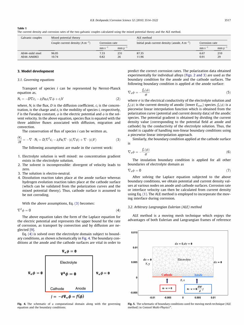
Table 1The current density and corrosion rates of the two galvanic couples calculated using the mixed potential theory and the ALE method.

Galvanic couples Mixed potential theory ALE method

Couple current density (A m�2) Corrosion rate Initial peak current density (anode, A m�2) Corrosion rate

nm s�1 mm y�1 nm s�1 mm y�1

AE44–mild steel 96.05 7.33 231 87.35 6.67 210AE44–AA6063 10.74 0.82 26 11.96 0.91 29

K.B. Deshpande / Corrosion Science 52 (2010) 3514–3522 3517

3. Model development

3.1. Governing equations

Transport of species i can be represented by Nernst-Planckequation as,

Ni ¼ �Drci � ziFuicir/þ ciV ð2Þ

where, Ni is the flux, D is the diffusion coefficient, ci is the concen-tration, is the charge and zi is the mobility of species i, respectively,F is the Faraday constant, / is the electric potential and / is the sol-vent velocity. In the above equation, species flux is equated with thethree additive fluxes associated with diffusion, migration andconvection.

The conservation of flux of species i can be written as,

@ci

@t¼ �r � Ni ¼ Dir2ci � ziFuir � ðcir/Þ þ r � ðciVÞ ð3Þ

The following assumptions are made in the current work:

1. Electrolyte solution is well mixed: no concentration gradientexists in the electrolyte solution.

2. The solvent is incompressible: divergent of velocity leads tozero.

3. The solution is electro-neutral.4. Dissolution reaction takes place at the anode surface whereas

hydrogen evolution reaction takes place at the cathode surface(which can be validated from the polarization curves and themixed potential theory). Thus, cathode surface is assumed tobe not corroding.

With the above assumptions, Eq. (3) becomes:

r2/ ¼ 0 ð4Þ

The above equation takes the form of the Laplace equation forthe electric potential and represents the upper bound for the rateof corrosion, as transport by convection and by diffusion are ne-glected [9].

Eq. (4) is solved over the electrolyte domain subject to bound-ary conditions, as shown schematically in Fig. 4. The boundary con-ditions at the anode and the cathode surfaces are vital in order to

Fig. 4. The schematic of a computational domain along with the governingequation and the boundary conditions.

predict the correct corrosion rates. The polarization data obtainedexperimentally for individual alloys (Figs. 2 and 3) are used as theboundary condition for the anode and the cathode surfaces. Thefollowing boundary condition is applied at the anode surface:

rn/ ¼ �fað/Þr ð5Þ

where r is the electrical conductivity of the electrolyte solution andfað/Þ is the current density of anodic (lower Ecorr) species. fað/Þ is apiecewise linear interpolation function which is obtained from thepolarization curve (potential and current density data) of the anodicspecies. The potential gradient is obtained by dividing the currentdensity value (corresponding to the potential field at anode andcathode) by the conductivity of the electrolyte solution. Thus, themodel is capable of handling non-linear boundary conditions usinga piecewise linear interpolation approach.

Similarly, the boundary condition applied at the cathode surfaceis

rn/ ¼ �fcð/Þr

ð6Þ

The insulation boundary condition is applied for all otherboundaries of electrolyte domain as

rn/ ¼ 0 ð7Þ

After solving the Laplace equation subjected to the aboveboundary conditions, we obtain potential and current density val-ues at various nodes on anode and cathode surfaces. Corrosion rateor interface velocity can then be calculated from current densityusing Eq. (1). The ALE method is employed to incorporate the mov-ing interface during corrosion.

3.2. Arbitrary Langrangian Eulerian (ALE) method

ALE method is a moving mesh technique which enjoys theadvantages of both Eulerian and Langrangian frames of reference

Fig. 5. The schematic of boundary conditions used for moving mesh technique (ALEmethod) in Comsol Multi-Physics�.

3518 K.B. Deshpande / Corrosion Science 52 (2010) 3514–3522

and can capture greater deformation with higher resolution [21].ALE method comprises of two frames: a reference frame withX, Y co-ordinates for a 2-D formulation and a spatial frame withx, y co-ordinates. The reference frame has fixed co-ordinates whilethe spatial frame has co-ordinates moving with time, subject toboundary conditions. We incorporate the ALE method using COM-SOL MultiPhysics�. The geometry and boundary conditions consid-ered for this moving mesh technique are shown in Fig. 5.

In COMSOL MultiPhysics�, the mesh displacement is obtainedby solving the following equations:

@2

@X2

@x@tþ @2

@Y2

@x@t¼ 0 and

@2

@X2

@y@tþ @2

@Y2

@y@t¼ 0 ð8Þ

The above equations dictate smooth deformation of the meshconsidering the constraints placed on the boundaries. The normalcomponent n of velocity vector v of the anode surface is calculatedusing Eq. (1) and represented as

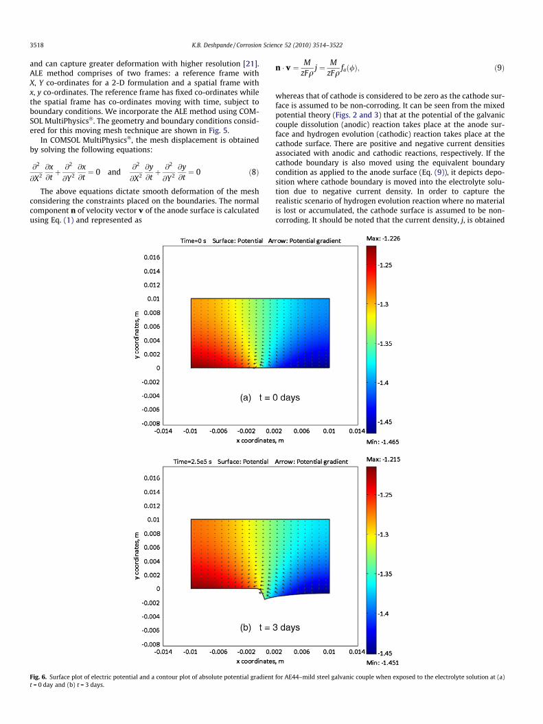
Fig. 6. Surface plot of electric potential and a contour plot of absolute potential gradientt = 0 day and (b) t = 3 days.

n � v ¼ MzFq

j ¼ MzFq

fað/Þ; ð9Þ

whereas that of cathode is considered to be zero as the cathode sur-face is assumed to be non-corroding. It can be seen from the mixedpotential theory (Figs. 2 and 3) that at the potential of the galvaniccouple dissolution (anodic) reaction takes place at the anode sur-face and hydrogen evolution (cathodic) reaction takes place at thecathode surface. There are positive and negative current densitiesassociated with anodic and cathodic reactions, respectively. If thecathode boundary is also moved using the equivalent boundarycondition as applied to the anode surface (Eq. (9)), it depicts depo-sition where cathode boundary is moved into the electrolyte solu-tion due to negative current density. In order to capture therealistic scenario of hydrogen evolution reaction where no materialis lost or accumulated, the cathode surface is assumed to be non-corroding. It should be noted that the current density, j, is obtained

for AE44–mild steel galvanic couple when exposed to the electrolyte solution at (a)

K.B. Deshpande / Corrosion Science 52 (2010) 3514–3522 3519

using a piecewise linear interpolation function, fað/Þ, as discussedin Eq. (5). All other boundaries are considered to have zero dis-placement.

4. Results and discussion

The ALE method, for the first time, is applied to investigate thecorrosion behaviour of AE44 (Mg) – mild steel couple which is ex-posed to 1.6 wt.% NaCl (electrolyte) solution. The change in electricpotential over the electrolyte domain obtained after solving the La-place equation for the electric potential is shown in Fig. 6 at timet = 0 and 3 days of continuous exposure to the electrolyte solution.It can be seen that the electric potential varies from �1.23 V(SCE)over the cathodic region to �1.47 V(SCE) over the anodic regionat time t = 0. It should be noted that the potential of the same gal-vanic couple is estimated to be �1.35 V(SCE) using the mixed po-tential theory, as seen in Fig. 2. The potential gradient is alsoshown in Fig. 6 in the form of arrows overlaid on the surface plotof the electric potential, which indicates the electric field inducedfrom the lower potential region (anode) to the higher potential re-gion (cathode). This electric field drives the dissolution of Mg intothe electrolyte solution. The contour plot of the absolute potentialgradient indicates the current density is the highest at the junctionof dissimilar materials, as seen in Fig. 6. This leads to a higher dis-solution of Mg at the junction and the dissolution rate decreasesalong the distance away from the junction eventually forming apit at the junction.

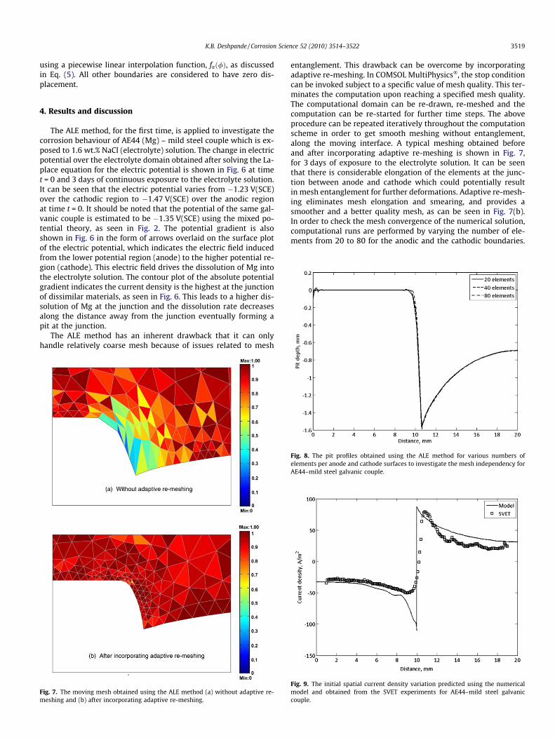
The ALE method has an inherent drawback that it can onlyhandle relatively coarse mesh because of issues related to mesh

Fig. 7. The moving mesh obtained using the ALE method (a) without adaptive re-meshing and (b) after incorporating adaptive re-meshing.

entanglement. This drawback can be overcome by incorporatingadaptive re-meshing. In COMSOL MultiPhysics�, the stop conditioncan be invoked subject to a specific value of mesh quality. This ter-minates the computation upon reaching a specified mesh quality.The computational domain can be re-drawn, re-meshed and thecomputation can be re-started for further time steps. The aboveprocedure can be repeated iteratively throughout the computationscheme in order to get smooth meshing without entanglement,along the moving interface. A typical meshing obtained beforeand after incorporating adaptive re-meshing is shown in Fig. 7,for 3 days of exposure to the electrolyte solution. It can be seenthat there is considerable elongation of the elements at the junc-tion between anode and cathode which could potentially resultin mesh entanglement for further deformations. Adaptive re-mesh-ing eliminates mesh elongation and smearing, and provides asmoother and a better quality mesh, as can be seen in Fig. 7(b).In order to check the mesh convergence of the numerical solution,computational runs are performed by varying the number of ele-ments from 20 to 80 for the anodic and the cathodic boundaries.

Fig. 8. The pit profiles obtained using the ALE method for various numbers ofelements per anode and cathode surfaces to investigate the mesh independency forAE44–mild steel galvanic couple.

Fig. 9. The initial spatial current density variation predicted using the numericalmodel and obtained from the SVET experiments for AE44–mild steel galvaniccouple.

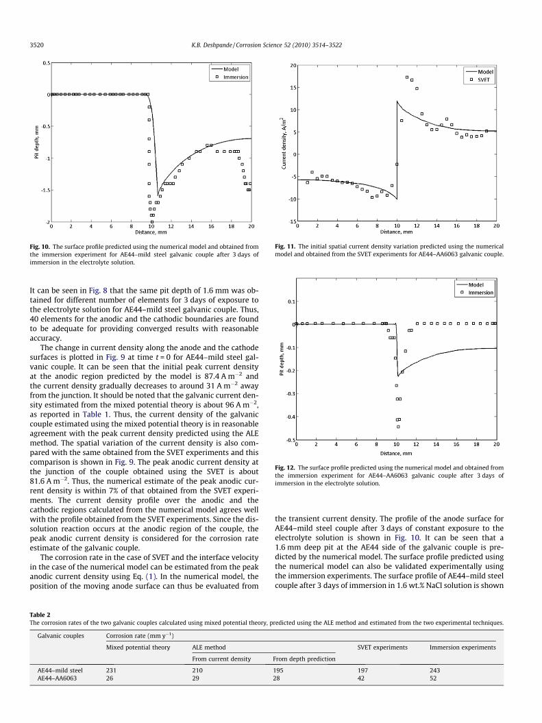
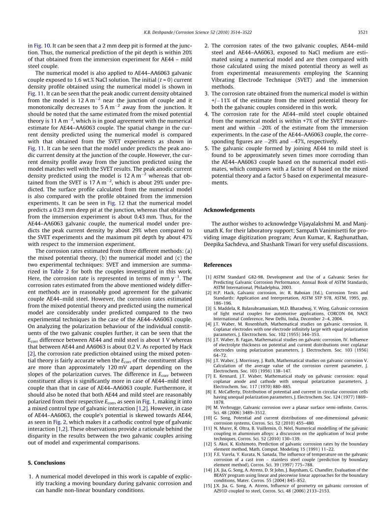
Fig. 10. The surface profile predicted using the numerical model and obtained fromthe immersion experiment for AE44–mild steel galvanic couple after 3 days ofimmersion in the electrolyte solution.

Fig. 11. The initial spatial current density variation predicted using the numericalmodel and obtained from the SVET experiments for AE44–AA6063 galvanic couple.

Fig. 12. The surface profile predicted using the numerical model and obtained fromthe immersion experiment for AE44–AA6063 galvanic couple after 3 days ofimmersion in the electrolyte solution.

3520 K.B. Deshpande / Corrosion Science 52 (2010) 3514–3522

It can be seen in Fig. 8 that the same pit depth of 1.6 mm was ob-tained for different number of elements for 3 days of exposure tothe electrolyte solution for AE44–mild steel galvanic couple. Thus,40 elements for the anodic and the cathodic boundaries are foundto be adequate for providing converged results with reasonableaccuracy.

The change in current density along the anode and the cathodesurfaces is plotted in Fig. 9 at time t = 0 for AE44–mild steel gal-vanic couple. It can be seen that the initial peak current densityat the anodic region predicted by the model is 87.4 A m�2 andthe current density gradually decreases to around 31 A m�2 awayfrom the junction. It should be noted that the galvanic current den-sity estimated from the mixed potential theory is about 96 A m�2,as reported in Table 1. Thus, the current density of the galvaniccouple estimated using the mixed potential theory is in reasonableagreement with the peak current density predicted using the ALEmethod. The spatial variation of the current density is also com-pared with the same obtained from the SVET experiments and thiscomparison is shown in Fig. 9. The peak anodic current density atthe junction of the couple obtained using the SVET is about81.6 A m�2. Thus, the numerical estimate of the peak anodic cur-rent density is within 7% of that obtained from the SVET experi-ments. The current density profile over the anodic and thecathodic regions calculated from the numerical model agrees wellwith the profile obtained from the SVET experiments. Since the dis-solution reaction occurs at the anodic region of the couple, thepeak anodic current density is considered for the corrosion rateestimate of the galvanic couple.

The corrosion rate in the case of SVET and the interface velocityin the case of the numerical model can be estimated from the peakanodic current density using Eq. (1). In the numerical model, theposition of the moving anode surface can thus be evaluated from

Table 2The corrosion rates of the two galvanic couples calculated using mixed potential theory, p

Galvanic couples Corrosion rate (mm y�1)

Mixed potential theory ALE method

From current density

AE44–mild steel 231 210AE44–AA6063 26 29

the transient current density. The profile of the anode surface forAE44–mild steel couple after 3 days of constant exposure to theelectrolyte solution is shown in Fig. 10. It can be seen that a1.6 mm deep pit at the AE44 side of the galvanic couple is pre-dicted by the numerical model. The surface profile predicted usingthe numerical model can also be validated experimentally usingthe immersion experiments. The surface profile of AE44–mild steelcouple after 3 days of immersion in 1.6 wt.% NaCl solution is shown

redicted using the ALE method and estimated from the two experimental techniques.

SVET experiments Immersion experiments

From depth prediction

195 197 24328 42 52

K.B. Deshpande / Corrosion Science 52 (2010) 3514–3522 3521

in Fig. 10. It can be seen that a 2 mm deep pit is formed at the junc-tion. Thus, the numerical prediction of the pit depth is within 20%of that obtained from the immersion experiment for AE44 – mildsteel couple.

The numerical model is also applied to AE44–AA6063 galvaniccouple exposed to 1.6 wt.% NaCl solution. The initial (t = 0) currentdensity profile obtained using the numerical model is shown inFig. 11. It can be seen that the peak anodic current density obtainedfrom the model is 12 A m�2 near the junction of couple and itmonotonically decreases to 5 A m�2 away from the junction. Itshould be noted that the same estimated from the mixed potentialtheory is 11 A m�2, which is in good agreement with the numericalestimate for AE44–AA6063 couple. The spatial change in the cur-rent density predicted using the numerical model is comparedwith that obtained from the SVET experiments as shown inFig. 11. It can be seen that the model under predicts the peak ano-dic current density at the junction of the couple. However, the cur-rent density profile away from the junction predicted using themodel matches well with the SVET results. The peak anodic currentdensity predicted using the model is 12 A m�2 whereas that ob-tained from the SVET is 17 A m�2, which is about 29% under pre-dicted. The surface profile calculated from the numerical modelis also compared with the profile obtained from the immersionexperiments. It can be seen in Fig. 12 that the numerical modelpredicts a 0.23 mm deep pit at the junction, whereas that obtainedfrom the immersion experiment is about 0.43 mm. Thus, for theAE44–AA6063 galvanic couple, the numerical model under pre-dicts the peak current density by about 29% when compared tothe SVET experiments and the maximum pit depth by about 47%with respect to the immersion experiment.

The corrosion rates estimated from three different methods: (a)the mixed potential theory, (b) the numerical model and (c) thetwo experimental techniques: SVET and immersion are summa-rized in Table 2 for both the couples investigated in this work.Here, the corrosion rate is represented in terms of mm y�1. Thecorrosion rates estimated from the above mentioned widely differ-ent methods are in reasonably good agreement for the galvaniccouple AE44–mild steel. However, the corrosion rates estimatedfrom the mixed potential theory and predicted using the numericalmodel are considerably under predicted compared to the twoexperimental techniques in the case of the AE44–AA6063 couple.On analyzing the polarization behaviour of the individual constit-uents of the two galvanic couples further, it can be seen that theEcorr difference between AE44 and mild steel is about 1 V whereasthat between AE44 and AA6063 is about 0.2 V. As reported by Hack[2], the corrosion rate prediction obtained using the mixed poten-tial theory is fairly accurate when the Ecorr of the constituent alloysare more than approximately 120 mV apart depending on theslopes of the polarization curves. The difference in Ecorr betweenconstituent alloys is significantly more in case of AE44–mild steelcouple than that in case of AE44–AA6063 couple. Furthermore, itshould also be noted that both AE44 and mild steel are reasonablypolarized from their respective Ecorr, as seen in Fig. 1, making it intoa mixed control type of galvanic interaction [1,2]. However, in caseof AE44–AA6063, the couple’s potential is skewed towards AE44,as seen in Fig. 2, which makes it a cathodic control type of galvanicinteraction [1,2]. These observations provide a rationale behind thedisparity in the results between the two galvanic couples arisingout of model and experimental comparisons.

5. Conclusions

1. A numerical model developed in this work is capable of explic-itly tracking a moving boundary during galvanic corrosion andcan handle non-linear boundary conditions.

2. The corrosion rates of the two galvanic couples, AE44–mildsteel and AE44–AA6063, exposed to NaCl medium are esti-mated using a numerical model and are then compared withthose calculated using the mixed potential theory as well asfrom experimental measurements employing the ScanningVibrating Electrode Technique (SVET) and the immersionmethods.

3. The corrosion rate obtained from the numerical model is within+/�11% of the estimate from the mixed potential theory forboth the galvanic couples considered in this work.

4. The corrosion rate for the AE44–mild steel couple obtainedfrom the numerical model is within +7% of the SVET measure-ment and within �20% of the estimate from the immersionexperiments. In the case of the AE44–AA6063 couple, the corre-sponding figures are �29% and �47%, respectively.

5. The galvanic couple formed by joining AE44 to mild steel isfound to be approximately seven times more corroding thanthe AE44–AA6063 couple based on the numerical model esti-mates, which compares with a factor of 8 based on the mixedpotential theory and a factor 5 based on experimental measure-ments.

Acknowledgements

The author wishes to acknowledge Vijayalakshmi M. and Manj-unath K. for their laboratory support; Sampath Vanimisetti for pro-viding image digitization program; Arun Kumar, K. Raghunathan,Deepika Sachdeva, and Shashank Tiwari for very useful discussions.

References

[1] ASTM Standard G82-98, Development and Use of a Galvanic Series forPredicting Galvanic Corrosion Performance, Annual Book of ASTM Standards,ASTM International, Philadelphia, 2003.

[2] H.P. Hack, Galvanic corrosion, in: R. Baboian (Ed.), Corrosion Tests andStandards: Application and Interpretation, ASTM STP 978, ASTM, 1995, pp.186–196.

[3] S. Maddela, R. Balasubramaniam, M.D. Bharadwaj, Y. Wing, Galvanic corrosionof light metal couples for automotive applications, CORCON 04, NACEInternational Conference, New Delhi, India, December 2–4, 2004.

[4] J.T. Waber, M. Rosenbluth, Mathematical studies on galvanic corrosion, II.Coplanar electrodes with one electrode infinitely large with equal polarizationparameters, J. Electrochem. Soc. 102 (1955) 344–353.

[5] J.T. Waber, B. Fagan, Mathematical studies on galvanic corrosion, IV. Influenceof electrolyte thickness on potential and current distributions over coplanarelectrodes using polarization parameters, J. Electrochem. Soc. 103 (1956)64–72.

[6] J.T. Waber, J. Morrissey, J. Ruth, Mathematical studies on galvanic corrosion V.Calculation of the average value of the corrosion current parameter, J.Electrochem. Soc. 103 (1956) 138–147.

[7] E. Kennard, J.T. Waber, Mathematical study on galvanic corrosion: equalcoplanar anode and cathode with unequal polarization parameters, J.Electrochem. Soc. 117 (1970) 880–885.

[8] E. McCafferty, Distribution of potential and current in circular corrosion cellshaving unequal polarization parameters, J. Electrochem. Soc. 124 (1977) 1869–1878.

[9] M. Verbrugge, Galvanic corrosion over a planar surface semi-infinite, Corros.Sci. 48 (2006) 3489–3512.

[10] G. Song, Potential and current distributions of one-dimensional galvaniccorrosion systems, Corros. Sci. 52 (2010) 455–480.

[11] N. Murer, R. Oltra, B. Vuillemin, O. Néel, Numerical modelling of the galvaniccoupling in aluminium alloys: a discussion on the application of local probetechniques, Corros. Sci. 52 (2010) 130–139.

[12] S. Akoi, K. Kishimoto, Prediction of galvanic corrosion rates by the boundaryelement method, Math. Comput. Modeling 15 (1991) 11–22.

[13] F.E. Varela, Y. Kurata, N. Sanada, The influence of temperature on the galvaniccorrosion of a cast iron – stainless steel couple (prediction by boundaryelement method), Corros. Sci. 39 (1997) 775–788.

[14] J.X. Jia, G. Song, A. Atrens, D. St John, J. Baynham, G. Chandler, Evaluation of theBEASY program using linear and piecewise linear approaches for the boundaryconditions, Mater. Corros. 55 (2004) 845–852.

[15] J.X. Jia, G. Song, A. Atrens, Influence of geometry on galvanic corrosion ofAZ91D coupled to steel, Corros. Sci. 48 (2006) 2133–2153.

3522 K.B. Deshpande / Corrosion Science 52 (2010) 3514–3522

[16] J.X. Jia, G. Song, A. Atrens, Experimental measurement and computersimulation of galvanic corrosion of magnesium coupled to steel, Adv. Eng.Mat. 9 (2007) 65–74.

[17] M. Bharadwaj, S. Thamida, S. Tiwari, in: Eighth International Symposium onAdvances in Electrochemical Science and Technology, November 28–30, 2006,Goa, India.

[18] K.B. Deshpande, Experimental investigation of galvanic corrosion: comparisonbetween SVET and immersion techniques, Corros. Sci. (2010), doi:10.1016/j.corsci.2010.04.023.

[19] ASTM Standard G102-89, Calculation of Corrosion Rates and RelatedInformation from Electrochemical Measurements, Annual Book of ASTMStandards, ASTM International, Philadelphia, 2004.

[20] W. S. Tait, An Introduction to Electrochemical Corrosion Testing for PracticingEngineers and Scientist, PairODocs Publications, Racine, WI, 1994.

[21] J. Donea, A. Huerta, J.-Ph. Ponthot, A. Rodriguez-Ferran, Arbitrary Lagrangian –Eulerian methods, in: E. Stein, R. de Borst, T.J.R. Hughes (Eds.), Encyclopedia ofComputational Mechanics, vol. 1, Fundamentals, John Wiley and Sons Ltd.,2004, pp. 1–25 (Chapter 14).

本文献由“学霸图书馆-文献云下载”收集自网络，仅供学习交流使用。

学霸图书馆（www.xuebalib.com）是一个“整合众多图书馆数据库资源，

提供一站式文献检索和下载服务”的24 小时在线不限IP

图书馆。

图书馆致力于便利、促进学习与科研，提供最强文献下载服务。

图书馆导航：

图书馆首页 文献云下载 图书馆入口 外文数据库大全 疑难文献辅助工具