Embed Size (px)
Citation preview

REPORT DOCUMENTATION PAGE Form Approved
OMB NO. 0704-0188
Public Reporting burden for this collection of information is estimated to average 1 hour per response, including the time for reviewing instructions, searching existing data sources, gathering and maintaining the data needed, and completing and reviewing the collection of information. Send comment regarding this burden estimates or any other aspect of this collection of information, including suggestions for reducing this burden, to Washington Headquarters Services, Directorate for information Operations and Reports, 1215 Jefferson Davis Highway, Suite 1204, Arlington, VA 22202-4302, and to the Office of Management and Budget, Paperwork Reduction Project (0704-0188,) Washington, DC 20503.
. AGENCY USE ONLY (Leave Blank) 2. REPORT DATE
December 20,2004
3. REPORT TYPE AND DATES COVERED
Final, 10/1/01 - 9/30/04
4. TITLE AND SUBTITLE
STUDY OF IN-CYLINDER REACTIONS OF HIGH POWER-DENSITY DIRECT INJECTION DIESEL ENGINES
5. FUNDING NUMBERS
6. AUTHOR(S)
M. Jansons, S. Lin and K. T. Rhee DAAD19-01-1-0766
7. PERFORMING ORGANIZATION NAME(S) AND ADDRESS(ES)
Rutgers, The State University of New Jersey Piscataway, NJ 08855-0909
8. PERFORMING ORGANIZATION REPORT NUMBER
9. SPONSORING / MONITORING AGENCY NAME(S) AND ADDRESS(ES)
U. S. Army Research Office P.O.Box 12211 Research Triangle Park, NC 27709-2211
10. SPONSORING / MONITORING AGENCY REPORT NUMBER
V3./fr?, £-£6 11. SUPPLEMENTARY NOTES
The views, opinions and/or findings contained in this report are those of the author(s) and should not be construed as an official Department of the Army position, policy or decision, unless so designated by other documentation.
12 a. DISTRIBUTION / AVAILABILITY STATEMENT
Approved for public release; distribution unlimited.
12 b. DISTRIBUTION CODE
13. ABSTRACT (Maximum 200 words)
Direct-injection (DI) Diesel or compression-ignition (CI) engine combustion process is investigated when new design and operational strategies are employed in order to achieve a high power-density (HPD) engine. This goal is being achieved by developing quantitative imaging and speciation methods of in-cylinder reaction processes.
Main achievements made during the course of the present study included: Construction/development and implementation of (1) a digital imaging system consisting of five (5) units of high-speed cryogenically cooled infrared focal plane arrays operated by a single electronic-control-package, (2) a four-color-artificial intelligence method (FCAIM); (3) an optical DI-CI engine, (4) Rutgers Animation Program (RAP); (5) new electronic packages for imaging system; (6) vector weighted flame analysis for evaluating stability of in-cylinder reactions; (7) a new spectrometer and (8) a new HITRAN data base gas radiation model replacing our earlier model based on NASA IR handbook.
A typical set of final results in the study is quantitative images (distributions of water vapor, soot, gas temperature and cylinder wall temperature at successive instants of time during the reaction period, which are obtained from the consecutive cycles. They are also further analyzed stability of flame propagations (e.g., repeatability) by using the vector weighted (special- and intensity-weighted analysis) to access the high-power density engine operations.
14. SUBJECT TERMS
Super Imaging System, High-speed Imaging, Spectral Infrared Imaging, Vector-weighted Flame analysis, Consecutive-Cycle Imaging, Infrared Spectrometer, Four-color Method
15. NUMBER OF PAGES
62
16. PRICE CODE
17. SECURITY CLASSIFICATION OR REPORT
UNCLASSIFIED
18. SECURITY CLASSIFICATION ON THIS PAGE
UNCLASSIFIED
19. SECURITY CLASSIFICATION OF ABSTRACT
UNCLASSIFIED
20. LIMITATION OF ABSTRACT
UL NSN 7540-01-280-5500 Standard Form 298 (Rev.2-89)
Prescribed by ANSI Std. 239-18 298-102
Enclosure 1

TABLE OF CONTENTS
Page
Cover Page
Table of Contents
1. Introduction 1 2. Main Achievement 2 3. Description of Results 3
3-1. Construction of Electro-Optical System (Hardware) 3 3-2. High-speed Imaging from Successive Cycles 6 3-3. Quantitative Imaging - Artificial Intelligence Four-color Method 7 3-4. Analysis of Cyclic Stability of Flame Propagation -
Characteristic Vector Set Method 12 3-5. New Optical Engine Apparatus 13 3-6. Hitran Replacing NASA Group Line Model 15
4. Summary 15 5. References 15
Appendix 18
Appendix-1. Operating System of SIS-EFS 18 Appendix-2. Artificial Intelligence Four-color Method (AIFCM) 26
A-2-1. Four-dimensional Spectrometric Method Setup 26 A-2-2. Artificial Intelligence Four-color Method 27
A. Concept of Artificial Intelligent Four Color Method (AIFCM) B. Relational Entity of Four Color Method C. Partition the Variable Space
Appendix-3. Stability Analysis using Vector Defined Characteristics 34
A-3-1. Characteristic Vector Set in Continuous Form 34 A-3-2. CaseStudy-I 37 A-3-3. Application to Engine Flame 40
Appendix-4. HITRAN - Gas Radiation Models
A-4-1. Line-by-Line Radiation Model using HITRAN Data base 46
20050201 032
Final Report
Study of In-cylinder Reactions of High Power-density Direct-injection Diesel Engines
(ARO Contract No. DAAD 19-01-1-0766)
KTRhee Department of Mechanical and Aerospace Engineering
Rutgers, The State University of New Jersey
1. INTRODUCTION
More power output from smaller engines producing low emissions is desired. Development of such high power-density (HPD) direct-injection compression-ignition (DI-CI) or Diesel engines in Army's ground vehicles is explored by employing low air-fuel-ratio combustion, low heat-rejection (LHR), high-speed, two-cycle operation, and others.
These strategies for HPD engine design become more promising when melded, in the conventional CI-engine-base, with high-performance fuel injection (HPFI), advanced design and materials, and tribology improvement. In particular, modern technology advancements in the electro-mechanical areas shed a better light into the processes of achieving the goal of HPD DI-CI.
Among the problems faced in this challenging work is clearly control of the combustion process. For example, a high-speed operation and LHR result in both a shortened physical time for mixing and increased intake air temperature. They necessitate an enhanced induction air management (e.g. cooling and turbocharging) and better fuel delivery (by using an HPFI). Those measures would help lead to a low-smoke-emission high-efficiency HPD by implementing a better control of fuel- air distribution and preflame reactions prior to the onset of an abrupt combustion stage.
In-cylinder DI-CI reaction processes, which dictate the success of the HPD engine design, are often significantly altered when even a seemingly simple design parameter is changed, affecting both engine output and emissions. A better understanding of the impacts of HPD system basics, therefore, would be a precondition for achieving successful engine development Desirably, since the cut-and-try development approach is costly, it necessitates a more realistic model to predict the behavior of Diesel flames in turbulent, high-speed, high-temperature and high-pressure environments subject to the wide range of operating parameters experienced by vehicle powerplants. There is a pressing need for a tool capable of validating any proposed combustion model by observing realistic combustion in details consistent with new engine design strategies.
The present work was to develop a comprehensive combustion analysis tool, capable of extracting data from the HPD engine cylinder under real-world conditions. The new tool, then, was to be employed in order to achieve the goal of investigating HPD engine in-cylinder processes and accumulation of extensive amounts of data to help verify combustion models, as mentioned above.

Importance of the Present Work. Modern advancements in sensor and information handling technologies have recently enhanced both the extent and depth of scientific research and product development. In amounts unthinkable even several years ago! For example, the point measurement is rapidly replaced by (simultaneous) acquisition of arrays of the same results, such data matrices are sequentially captured, and the same quantitative imaging can be implemented in huge amounts at high rates (thanks to high-speed affordable memory and powerful I/O and A/D peripheral devices).
For example, what is achieved by the conventional methods (such as high-speed photography) permits investigation of (transient in-cylinder) reactions typically in a single cycle at a time. Often such investigation is only possible within the first several cycles from the start (before the optical window is covered by soot). The new research tool that was developed under the present work was to overcome much of such limitations by employing the most advanced peripheral devices combined with the conventional optical-spectrometric technologies. The new diagnostic tool permits simultaneously capturing digital spectral images of transient thermochemical reactions with their corresponding spectral characteristics. The system was developed to successively obtain such results from the very first start of ignition to over 100 continuous cycles. A new method to review-analyze vast amounts of digital movies produced by the tool has also been developed.
2. MAINACHIEVMENT
Results obtained from the present work are briefly discussed in both apparatus (engine and diagnostic devices) and processing computer programs below and details of individual topics are explained later.
Tool Development. A multi-spectral digital imaging system (hardware, called Super Imaging System, SIS) incorporated with high-speed massive data methods as a research tool was developed. The new tool became capable of simultaneously capturing both multiple spectral images and spectral distributions from many successive cycles. They are processed using new spectrometric methods in order to achieve quantitative imaging and speciation.
New Data Acquisition and Analysis/Presentation Methods. When the SIS is operated for obtaining imaging data and others (e.g. pressure-time history), it generates huge amounts of data (typically several hundred mega-bites in 12-bit dynamic depth in one set of experiment). A new operating system (OS) for the SIS was developed which is incorporated with data analysis/process methods as explained next.
New (Artificial Intelligence) Data-Analysis Methods. Raw data obtained using the SIS include four sets of geometrically identical digital images in respective spectral bands captured at the successive instants of time. Those unique sets of data matrixes offer new opportunities of determining quantitative imaging, i.e. distributions of temperature and species when the matching digital data are processed. It required an entirely new spectrometric method, namely four-color artificial intelligence methods.
New Spectrometer and Optical Data Analysis using Hitran. The SIS is incorporated with a newly designed/fabricated spectrometer towards a goal of speciation of the imaging area (in-
2

cylinder reactions). What is different in the present data analysis methods than the our earlier spectrometric data handling programs (loaded with 1972 NASA published Infrared Handbook data) is that the new one is based on the 2004 HITRAN Molecular Spectroscopic Database, which offers advantages over the former such as more species and finely discrete digital data (i.e., smaller intervals of wave numbers for corresponding absorptance).
Engine Apparatus Construction. In order to obtain a more real-world like engine apparatus and greater optical view of the in-cylinder processes, a new engine apparatus has been constructed by modifying a V-8 Cummins 903 engine. The construction of this apparatus required large amount of resources and time, and is anticipated to provide optical access to a commercial large-bore Diesel engine.
Findings. Results from the study are discussed in details when they are individually explained in the following.
3. DESCRIPTION OF RESULTS
Achievements are discussed in three areas, including the apparatus, data analysis/presentation computer programs, and respective results where deemed appropriate.
3-1. Construction of Electro-Optical System (Hardware)
The main diagnostic tool employed in the study is an extensively modified/improved system from four-color Infrared imaging system during the course of the present study. A portion of the system is designed for multi-spectral imaging and other portion is for obtaining spectra distribution of corresponding images (Fig. 1).
Rutgers Super Imaging System (SIS) and a New Spectrometer. As schematically depicted in the figure, radiation issued from reaction volume (e.g. the combustion chamber) is relayed to the object lens of the four-color IR imaging system.
This system includes five (5) units of high-speed infrared (IR) camera (cryogenically cooled focal plane array, FPA of PtSi, 128x64): Four units (FPA, 1-4) are lined up with a single optical train (the upper portion in Fig. 1), and another unit (FPA, 5) is a part of newly designed/fabricated spectrometer, which will be discussed later.
Main purposed of this arrangement include: (1) that it is to simultaneously capture (1) four geometrically identical images in respective spectral bands and (2) that it is to obtain a spectrally-resolved radiation, in a varied sub-range within the imaging range considered in (1), over FPA-5. These spectral digital images and the said spectra distribution are concurrently obtained at high rates from many consecutive cycles. Note that the entire system (including the SIS and spectrometer) is operated by the same package of electronic control units.

IR Camera-1 (FPA)
— (2.2(im) £ Cassagrain Assembly
ID IR Camera-2 (FPA)
(2.47nm)
^ Spectral Beam Splitters 1
IR Camera-3 (FPA)
>|G (3.8nm)
□ IR Camera-4 (FPA) (3.42nm)
I a
Ebert-Fastie Spectrometer
IR Camera-5 (FPA)
(Spectra Distribution for Speciation corresponding to Images Obtained in Camera-1 to -4)
Fig. 1. Rutgers New Super Imaging System and Ebert-Fastie Spectometer.
Goals of this system include determination of when, where and what species are formed during the reaction period. It was expected that the results obtained using this new system was to improve our understanding of in-cylinder processes and verify existing and future CI-DI engine combustion models.
Mentioning the new SIS development, it is the 4th generation SIS in a part of sequential efforts of improving/developing diagnostic tool. It is, in a sense, a series of learning and "catching-up-with" activities of the modern advancements in electronic and data handling technology. For example, when development of the 1st SIS was conceived, a state-of-the-art A/D module (10 MHz in 12-bit dynamic resolution) typically consumed 30 watts (requiring a forced cooling) opposed to only a fraction of watts in a comparable modern unit. Later, newly available programmable logic gate arrays (PLGAs) in the 2nd SIS replaced our complex and trouble-prone electronic packages made of numerous elements soldered over crowded hand-wired electronic boards composing the 1st SIS.
In order to improve high-speed data handling, next, entirely new modular control units (with individual A/D units) were introduced replacing a single control approach employed in the 2nd
generation system. This was, of course, facilitated by the PLGAs. Advancements of PLGAs, thereafter, became so significant that ironically we ran into some insurmountable difficulties. Simply, it became greatly difficult to find replacement parts (they became obsolete). Thus, in order to exploit new PLGA performance and to further the system reliability, we utilized know-how of the SIS development accumulated to date. At this time, electronic boards in the modules have newly been designed-fabricated by

NEWTONIAN UIRROR: 25.4 mm diameter
protected geld first surface GERMANIUM LENS:
-115 mm focal length, 1/ 2.3 2.1 - 5.5 pm bandwidth mB£ pLAm
negative grating orders
DIFFRACTION GRATING: 35 grooves/mm, 2,3368 deg blaze angle
26 x 26 mm blazed orsa
IMAGE PLANE: positive grating orders
SLIT HOLDER: 9.5 mm substrate diameter
variable slit width
WHITE LIGHT
2 pm WAVELENGTH
5 ftm WAVELENGTH
SPHERICAL MIRROR: 76.2 mm diometsr, f/1 protected aluminum first surface
Fig. 2. A New Ebert-Fastie Spectrometers and Its Ray Trace (the Lower Portion of Fig. 1).
an outside specialist that replace all in-house-laboratory-built electronic boards. This facilitates the flexibility and control of system performance, further aided by our new operation system (OS, software packages), as explained later.
Ebert-Fastie Spectrometer. When four sets of high-speed spectral images were taken, some unusual findings were obtained. For example, although they were captured from the same phenomena, matching images appeared dissimilar to each other, in particular, when those of diffusion flames were observed. It seemed to be a logical step to obtain spectra distributions of individual spectral images in order to identify causes of such difference by using a spectrometer.
Since the present one-of-a-kind SIS (with a tight space limitation) would not readily accommodate spectrometers available on the shelf, it is decided to newly design and fabricate the optical portion of the system as shown in Fig. 2 (refer to Fig 1). The basic idea of the mutual incorporation of the two is that a new spectrometer package is placed directly above the present SIS (without employing a separate beam splitter).
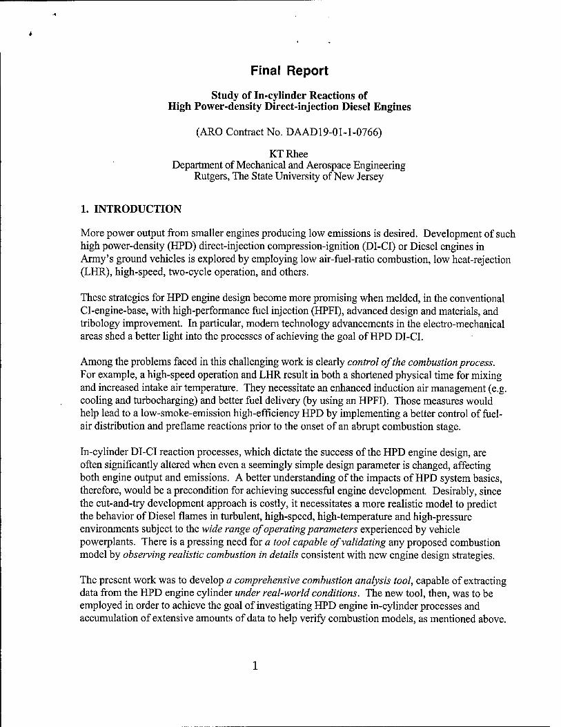
In determining the optical arrangement for the present spectrometer, out of two layouts, e.g., two-mirror Czerny-Turner vs. single-mirror Ebert-Fastie spectrometers, the latter was employed in the present design. Without elaborating development processes, it is noted that the optical layout has been fabricated third time over to date in order to achieve the most desirable performance under given space-system limitations (a new learning process). The new layout is expected to offer greater flexibility and adjustment capability in capturing spectra distributions over a choice of spectral range, which is further facilitated by incremental-multi-dimensional-relocation (adjustment) features of individual optical elements in the system. The SIS-spectrometer package is shown in Fig. 3.
The laboratory designed/fabricated spectrometer appears to be a stand-alone instrumentation capable of in-depth analytical investigation of thermochemical reaction phenomena. For example, alteration of a flame when some additives are introduced into its fuel or air would be more closely studied by using this new SIS-spectrometer package.
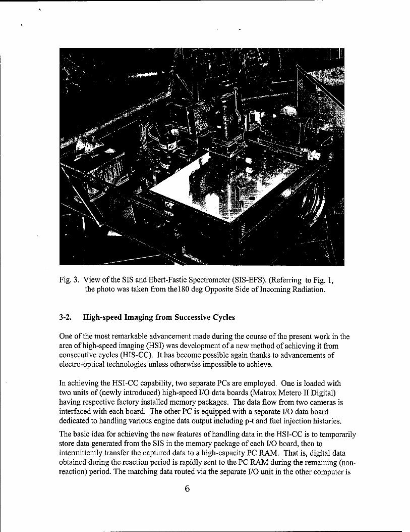
Fig. 3. View of the SIS and Ebert-Fastie Spectrometer (SIS-EFS). (Referring to Fig. 1, the photo was taken from the 180 deg Opposite Side of Incoming Radiation.
3-2. High-speed Imaging from Successive Cycles
One of the most remarkable advancement made during the course of the present work in the area of high-speed imaging (HSI) was development of a new method of achieving it from consecutive cycles (HIS-CC). It has become possible again thanks to advancements of electro-optical technologies unless otherwise impossible to achieve.
In achieving the HSI-CC capability, two separate PCs are employed. One is loaded with two units of (newly introduced) high-speed I/O data boards (Matrox Metero II Digital) having respective factory installed memory packages. The data flow from two cameras is interfaced with each board. The other PC is equipped with a separate I/O data board dedicated to handling various engine data output including p-t and fuel injection histories.
The basic idea for achieving the new features of handling data in the HSI-CC is to temporarily store data generated from the SIS in the memory package of each I/O board, then to intermittently transfer the captured data to a high-capacity PC RAM. That is, digital data obtained during the reaction period is rapidly sent to the PC RAM during the remaining (non- reaction) period. The matching data routed via the separate I/O unit in the other computer is

transferred to the same RAM at this time. The data acquisition in both computers is made by using the same timing signals generated from a single central clock and corresponding engine CA markers, which ensures the individual sets of data to be captured concurrently.
With this data management package, we are able to obtain either 64 or 128 successive images in each cycle per camera from over 150 consecutive cycles, which amounts to a data volume of approximately 400 mega bytes per experiment. Since this attempt has never been made in engine studies earlier, entirely new sub-circuit-boards, cables and software are constructed (for I/O units). Especially, an almost entirely new software package for this system is developed as explained in the next section.
Massive Information Handling (Software). When the above-mentioned new apparatus is employed for achieving the proposed extensiveness of investigating engines' transient combustion reactions, the typical volume of measurement (by using the new apparatus) is nearly 400 million data points (of 12-bit dynamic resolution) in each experiment. For example, when the cyclic behaviors of engine combustion are investigated, digital images in five FPAs are obtained (as high as nearly 2,000 frames/sec each) over 100 consecutive cycles.
Since such measurement is repeated (e.g. for investigating transient non-repetitive reactions), it was necessary not only to develop methods of handling the massive volumes of data but also of processing and analyzing the results. Development of new computer programs for manipulating data storage-retrieval-processing-analysis-dissemination was a challenging but essential part of the study. The program package includes: (1) Operating System (OS), and (2) Rutgers Animation Program.
Mentioning the OS, because of the complexity of data management during the experiment and the need for expedient control of individual experiment (also for in situ review of results) a new A/D module was placed in a PC (MS NT base) in order to direct the performance of the SIS- Ebert-Fastie Spectrometer (hereafter, called SIS-EFS). The entire system control computer programs were written in MS-C++. See Appendix-1.
3-3. Quantitative Imaging - Artificial Intelligence Four-color Method (AIFCM)
Unlike point-measurements made in various scientific/engineering studies, it is desired to have distributions of quantities (e.g., temperature and species concentration), which would minimize misleading judgments (like a blind-man's description of an elephant). The conception of the SIS was, in fact, to achieve such distributions, i.e., quantitative imaging. Several attempts have made in the past in order to process the governing equations to face difficulties in finding converging numbers in the numeric processing.
In discussing the issue, Fig. 3 illustrates some of main spectrometric methods developed for engine research, i.e. for point measurements and for determination of distributions (quantitative imaging by the present author) in a time-sequence. (A probable reason for the absence of latter activities by others is that the SIS is a one-of-a-kind unit so that no other research individual needed for developing such spectrometric methods for quantitative imaging.)
7
( Distril Distributions H20, Soot,
r u Four-color A. I.
Method (Lin & Rhee)
2003, Rutgers
Three-band ( Distributions^ iteration Method Vjg,H2Q, Sooy (Chang and Rhee)
1996, Rutgers I I
I I
New Band Ratio Method
(Chang and Rhee) 1995, Rutgers
' ^Distributions^ I ^ Tg,H20 ) I
I Distributions^
Tg, H20 ) Mapping Method
(Jiang and Rhee) 1990, Rutgers
1960 1970 1980 1990 1995 2000 2005
Fig. 4. IR Spectrometric Methods Applied to (Engine) Combustion Systems
Difficulties in Multi-spectral Methods. When the three-color iteration method (refer to the above chart) was developed, some considerable difficulties were encountered in finding the final solution, as mentioned above. As one may realize from the chart, it has been a rather long period of time since our attempt of three-color methods until our development of the recent four-color method, which was basically because of these difficulties. It was mainly due to the fact that in spite of the logical rigor of the governing equations (i.e., three simultaneous equations for three unknowns) the iteration often did not converge in some section of the (quantitative) image, which was then considered to stem from inaccurate raw data captured by the SIS. This consideration was found to lack in substance as discussed next.
During the course of developing our new four-color method, something quite unexpected was discovered: Let's consider a combustion environment as depicted in Fig. 4 where a volume of gaseous mixtures present in front of a surface at designated temperatures, species concentrations, optical path, and pressure.
Multiple Solutions. When respective spectral intensities (Lj) estimated for the above case (using the NASA IR Handbook, 1973) was introduced to our governing equations to see if our four-color method could reproduce the designated specifications, it was not the case to generate the same. There were multiple sets of solutions (hereafter called "results") for the same set of intensities. Sample results of (in units as shown in Fig. 5) water vapor-soot- wall temperature-mixture temperature included: 17.2-326.1-400-1200;
8

O Water Vapor (%) 12
• Soot (1.0 e-gg/cm3) 223
Wall Temperature (K) 510
Mixture Temperature (K) 1260
Path Length (cm) 23
Pressure (atm) 24
y Wall at T
fy-6 o / * *
*(K)
^w I,
J'o°°'-° ;. . O O
!.°.°.o f o .
%
Tg(K)
ll
L°o.° ■*3
1
ä ' o * < >-
^ 'A4
Fig. 5. Combustion Volume with Designated Specification (Left).
12.7-217.4-500-1267; 1.4-1.6-500-2167; and more (unlike what is shown in the chart). (Path length and pressure are assumed to stay the same) That is, the same set of spectral intensities is estimated for all combustion objects as those specified in respective groups of numbers. The main reasons for our inability of mathematically finding a converged set of solutions from our governing equations turned out to be due to the existence of such multiple solutions.
A New Strategy for Four-Color Method. In addition to existence of multiple results for the same set of spectral intensities, experimental error included in their measurements (by the SIS) would make implementation of a solution certainly more difficult. Consequently, an entirely new solution strategy is introduced in search of results as briefly explained next (More details are included in Appendix-2). It is to employ a vast-volume data-base in search of the result. The method would be therefore regarded as an artificial intelligence method.
First of all, a new data-base is generated for discrete numerical variations of parameters (i.e., results) within the ranges expected in typical combustion systems (for example, wall temperature varying from 300 to 900K, and water concentration ranging from 1 to 18%, etc.), which is to generate many sets of matching spectral intensities to be stored in the data-base.
In finding the solution for set of intensities within a given combustion environment, which is the reverse of the above, another unique methodology was introduced. For a set of spectral intensities (from experiment), in addition to all possible results, those matching to intensities encompassing a +/- 2.5% error are extracted from the data-base. The next task is to determine which set of those results is the exact and final out of multiple solutions.
Divide-and-Conquer. Figure 6 is introduced in explaining the next step to be taken. The large amount of results extracted from our new data-base for a given set of intensities

O Nearest Neighbors (Solutions from RU Data-base)
■ Possible Solution
Fig. 6. Divide-and-Conquer Strategy.
(plus a error range) is grouped with each of its nearest neighbors. Those groups are examined then to eliminate the unlikely ones by reflecting the combustion characteristics being considered. For example, it would be unlikely to have a high mixture temperature when water (product) concentration is very low. (Note that, in search of solution by an iteration method, when those near the lines dividing the groups are considered, the iteration process hardly comes to a converged result.)
After the elimination process, the solution is implemented for the measurement (without an error at this time) by limiting the range of results according to those identified within the final group, which then leads the iteration to rapidly converge to the final results.
Artificial Intelligence Four-Color Method (AIFCM). This brief description, however simple it might appear, involves some delicate technical challenges. For example, the division of results in nearest neighbors requires rigor and consistency. One of the methods explored for such area/domain subdivision problems may be the famous "postal office problem (Knuth, 1973)."
Briefly, it is to distribute sets of "postal offices" (sites) onto a planner area and then divid the area into subdivisions such that traveling from a certain point to a post office in the same division costs less than traveling to any other post offices in the area (e.g. Vornoi assignment model and Voronois diagram).
Basically, we consider all solutions of the FCAI as "sites." They consist of results, i.e., mixture temperature, wall temperature, plus water and soot concentrations. More details of the AIFCM are included in Appendix-2.
10

1 aTDC
3 aTDC
5 aTDC
7 aTDC
9 aTDC
11 aTDC
13 aTDC
15 aTDC
17 aTDC
19 aTDC
21 aTDC
23 aTDC
Spectral Image at 3.8 urn
Spectral Image at 2.2 urn
Spectral Image at 3.45 urn
Spectral Image at 2.47 um
Temperature Distribution
Water Vapor Distribution
Soot Concentration Distribution
Wall Temperature Distribution
Fig. 7. Quantitative Images obtained using AIFCM by Processing Spectral Images Captured using Rutgers SIS from an SI Engine Operated by Gasoline at a near Stoichiometric Fuel/air Ratio.
11

3.8um 2.2iiiii
513 1753 ' W/SR ■ W/SR
3.45 u m 651
W/SR
2.47 ii m 1698
1W/SR
1 0
■gas
1750K
[H20]
12.5%
|
300K
[soot]
3.5XKT
Twall
750K SM//CO l/DUK 1^.3.» -~«.» _z ijui
B I img'cm B
I 300 K
Sample Calculations. A set of spectral images obtained from a consecutive cycles of an SI engine operated by gasoline near a stoichiometric fuel/air ratio was processed to determine quantitative images by using the present AIFCM as included below. Note that the engine condition at which the present spectral images was acquired was found to be rather poor as discovered afterward. (The optical SI engine apparatus was constructed by converting a Ford V-8 engine to achieve an optical access via an extended piston with an Si- window at the top so that the full view of the cylinder head captured during the imaging process. This apparatus has drained considerable amount of time and resource recent months diverting our attention from our main goal of engine studies.)
3-4. Analysis of Cyclic Stability of Flame Propagation - Characteristic Vector Set Method
The repeatability of in-cylinder flame propagation at corresponding engine crank angles is a desirable property in achieving better engine performance characteristics. Such a property is important condition as a high-efficiency, smooth-running, low-emission, and simpler optimized engine package.
When high-speed spectral digital images are captured at consecutive cycles (e.g. 100 cycles), analysis of the timed-stability is possible, it would help design such a super engine. For achieving the goal, a new vector stability factor is formulated and applied to results from the present SIS.
Various methods have been developed in order to evaluate the stability of engine operations. Those methods, however, concentrate either on pressure/time data, heat release rate or on power produced, all of which are one dimensional in time scale.
For example, when using pressure as stability indicator, at a certain crank angle (CA), only one number is used to do the evaluation. For instance, if we compare two pressure points at the same CA for two different engine cycles, we may get a very similar value while the actual combustion processes vary tremendously.
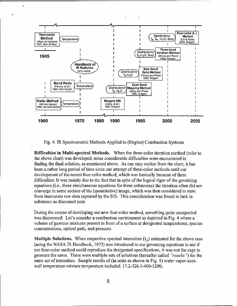
To symbolize this phenomenon, two geometrically different infrared profiles, yet producing the same pressure are displayed in Fig. 8. The use of pressure-time is not capable of distinguishing these two cases.
12
B /
Fig. 8. Two Geometrically Different Infrared Profiles with Same Pressure
The successful applications of the SIS in engine study give rise to a new direction of stability analysis. Since the SIS is capable of taking spatial infrared images, stability analysis can utilize spatial information along time scale. At a certain crank angle, we have 2D infrared profiles at our disposal. Studying the distribution of intensity profile can gain in depth knowledge into combustion itself.
This has called for the design of a new parameter to study engine stability using the time series 2D infrared profiles to better understand combustion and cyclic variations. Stability analysis in 2D space breaks down to compare similarity between different images. For engine running conditions, it is unlikely that two different infrared images at the same CA resemble each other perfectly, even for steady state conditions. In order to distinguish one image from another using our infrared imaging technology, fundamentally we will have to differentiate the following cases:
■ Geometric difference ■ Intensity difference ■
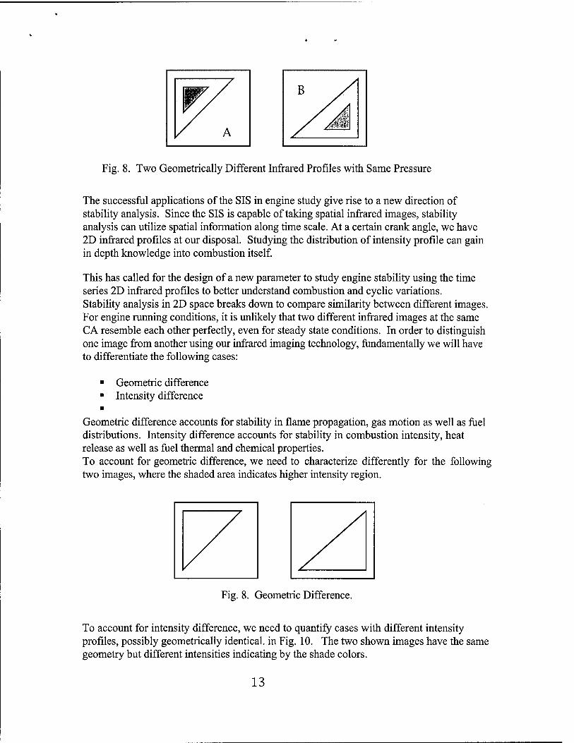
Geometric difference accounts for stability in flame propagation, gas motion as well as fuel distributions. Intensity difference accounts for stability in combustion intensity, heat release as well as fuel thermal and chemical properties. To account for geometric difference, we need to characterize differently for the following two images, where the shaded area indicates higher intensity region.
Fig. 8. Geometric Difference.
To account for intensity difference, we need to quantify cases with different intensity profiles, possibly geometrically identical, in Fig. 10. The two shown images have the same geometry but different intensities indicating by the shade colors.
13

Fig. 10. Intensity Difference
Comparison two images on a pixel-to-pixel basis is computationally expensive and the results are often over-sensitive. In addition, having comparative result for each pixel loses a comprehensive view of overall combustion process.
To overcome this problem, we need to design a new parameter that can account both for geometric difference as well as intensity difference. A new statistical analysis method has been developed as explained in Appendix-3.
3-5. New Optical Engine Apparatus
Unlikely the earlier optical-view-via-cylinder-head CI engine, a new optical-view-via-cylinder has been constructed. Among the advantages of this one over the former are a greater size of imaging view and zero modification of the cylinder head.
In spite of difficulties and a time-consuming design and fabrication process of this new apparatus, since its concept is well known, no further discussion on its construction is made here.
What is remarkable on the present approach, however, is that the present apparatus was being mated with a modern electronically controlled common-rail high-pressure fuel injection system (HPFI). Note that earlier studies were conducted by using our laboratory- built HPFI, which delivered as much as 207 MPa (30,000 psi). Recognizing considerable advancement of HPFI technology being made in the industry, at this time, in collaboration with Cummins Engine Co, their most advanced unit is introduced in the present study.
The expertise and experience in engine development added in this collaboration is an important asset in learning what is happening in the real-world "well tuned" CI-DI engine cylinder. For example, as briefly discussed earlier, even a simple alteration of injector variables (in an optimized engine) results in some dramatic deterioration of engine performance and emission characteristics. Such a change is not well known to engine designers at the present. It is critically important to find DI-CI physical/chemical processes resulting in such a shift, not only for engine designers but also for research individuals in the field.
A simple example in our collaborative work with the industry is in-cylinder measurements from our optical engine apparatuses, built to represent the real-world engines mated with an
14

optimized HPFI (for the engine), is compared with those from "not-so-optimized" engine environment as identified by Cummins designers.
3-5. HITRAN Model Replacing NASA Group Line Model
The analysis of observed combustion phenomena requires consideration of the interaction of electro-magnetic radiation and matter. These interactions play a role not only in the generation and self-absorption of radiation by gases within the combustion chamber itself, but also during propagation through the optical access window and optical path to the sensing equipment.
Gas radiation models are based on the quantum nature of these molecules and may be used to create a synthetic spectrum simulating that of combustion gases.
Earlier, we developed an analysis (Group Line Model) program utilizing NASA IR Handbook (Ludwig, et al., 1973). Thanks to introduction of HITRAN model available in the public domain, our entire analysis of gas radiation is being made using our new package employing HITRAN Model as explained in Appendix-4.
4. SUMMARY
Several main achievements have been made during the course of the present study as listed below. They are individually explained in both the text and appendix. It is expected to generate at lease four main publications from the results in near future.
(1) Construction of Electro-Optical System (Hardware) (2) High-speed Imaging from Successive Cycles (3) Quantitative Imaging - Artificial Intelligence Four-color Method (4) Analysis of Cyclic Stability of Flame Propagation - Characteristic Vector Set Method (5) New Optical Engine Apparatus (6) HITRAN Replacing NASA Group Line Model
5. REFERENCES
Bakenhus, Marco, Reitz, Rolf D., "Two-Color Combustion Visualization of Single and Split Injections in a Single-Cylinder heavy-duty D.I. Diesel Engine Using an Endoscope- Based Imaging System", SAE Paper 1999-01-1112,1999.
Bard, S. and Pagni, P.J., Carbon Particles in Small Pool Fire Flame," J. of Heat Transfer, vol. 103, pp. 357-362, 1981.
Campbell, S., Clasen, E., Chang, C, ad Rhee, K.T., "Flames and Liquid Fuel in an SI Engine during Cold Start," SAEPaper-961153,1996.
15

Chang, S.L. and Rhee, K.T., "Computation of Radiation Heat Transfer in Diesel Combustion," SAEPaper-831332,1983.
Clasen, E., Campbell, S., and Rhee, K.T., "Spectral IR Images of Direct-Injection Diesel Combustion by High-Pressure Fuel Injection," SAE Paper-950605,1995.
Clasen, E., Song, K., Campbell, S., and Rhee, K.T., "Fuel Effects on Diesel Combustion Processes," SAE Paper-962066,1996.
Conley, Robert T., Infrared Spectroscopy, p 171, Allyn and Bacon, Boston, 1966
Dalzel, W.H. and Sarofim, A.F., "Optical Constants of Soot and their Application to Heat Flux Calculation," ASME Trans, vol. 9, p. 100, 1969.
Dec, J. and Espey, C, "Chemiluminescence Imaging of Autoignition in a DI Diesel Engine," SAE Paper-982685, 1998.
Fischer, J.; Gamache, R.R.; Goldman, A.; Rothman, L.S.; Perrin, A.: Total Internal Partition Sums for Molecular Species in the 2000 Edition of the HITRAN Database, Journal of Quantitative Spectroscopy and Radiative Transfer, Volume 82, Issues 1-4, pg. 401-412, Elsevier Science Ltd, Great Britain, 2003
Fristrom, RM.,Flame Structure and Processes, Oxford University Press, 1995.
Herzberg, Gerhard: Molecular Spectra and Molecular Structure, D. Van Nostrand Company, Inc., New York, 1950
Heywood, J., Internal Combustion Engine Fundamentals, p 686, McGraw-Hill, 1988.
James, J.F.; Sternberg, R.S.: The Design of Optical Spectrometers, Chapman and Hall Ltd, London, 1969.
Knuth, Donald E., "The Art of Computer Programming, Vol. 3." Addisono-Wesley, 1973..
Ludwig, C.B., Malkmus, W., Reardon, J.E., Thomson, J.A.L., Handbook of Infrared Radiation from Combustion Gases," NASA SP-3080,1973.
McClatchkey, R.A.; Benedict, W.S.; Clough, S.A.; Burch, D.E.; Calfee, R.F.; Fox, K.; Rothman, L.S.; Garing, J.S.: AFRCL Atmospheric Absorption Line Parameter Compilation, Air Force Cambridge Research Laboratories Optical Physics Laboratory Project 7670, AFCRL.TR-73-0096, Environmental Research Papers, No. 434,1973
Modest, Michael F.: Radiative Heat Transfer, Academic Press, San Diego, California, 2003.
Modest, Michael F.: http://books.elsevier.eom/us//aeg/, Elsevier Academic Press Advanced Education Bookstore, Companion Web Site for Radiative Heat Transfer, 2004
16
Packan, Denis M.; Gessman, Richard J.; Pierrot, Laurent; Laux, Christophe, 0.; Kruger, Charles H.; Measurement and Modeling of OH, NO, and C02 Infrared Radiation in a Low Temperature Air Plasma, American Institute of Aeronautics and Astronautics AIAA 99- 3605,1999.
Palmer, Christopher: Diffraction Grating Handbook, Richardson Grating Laboratory, Rochester, New York, 2000.
Rothman, L.S. et ah The HITRAN Molecular Spectroscopic Database and HAWKS (HITRAN Atmospheric Workstation): 1996 Edition, Journal of Quantitative Spectroscopy and Radiative Transfer Vol. 60, No. 5, pp. 665-710, Elsevier Science Ltd, Great Britain, 1998.
Rothman, L.S. et ah The HITRAN Molecular Spectroscopic Database and HAWKS (HITRAN Atmospheric Workstation): 2004 Edition, Journal of Quantitative Spectroscopy and Radiative Transfer, Elsevier Science Ltd, Great Britain, 2005 (to be published).
Siegel, Robert, Howell, John: Thermal Radiation Heat Transfer Hemisphere Publishing Corporation -McGraw-Hill Book Company, New York, 1981.
Stewart, James E.: Infrared Spectroscopy, Marcel Dekker Inc., New York, 1970
Song, K., Clasen, E., Chang, C, Campbell, S., Rhee, K.T., "Post-flame Oxidation and Unburned Hydrocarbon in a Spark-ignition Engine," SAE Paper-952543,1995.
17

APPENDIX
Individual results briefly explained in the text are further explained in the following. This portion also serves as our reference manual.
In particular, it is emphasized that the all the details of the hardware connections and communication instructions in the machine language have been developed during the course of the present work.
Appendix-1. Operating System of SIS-EFS
The new Rutgers Animation Program (RAP) is considerably different from the earlier package in both depth and extent. It is, indeed, an integrated package of computer programs that include the SIS-EFS Operating System (OS), review-analysis-presentation programs of raw data, and software for processing data (e.g. new spectrometric methods) and presentation (together with the raw data). At this time the portion of OS is discussed first, which involves description of our A/D module and its manipulation.
A part of functions in the new software package is to manipulate an A/D acquisition board (PCT-DAS1000) loaded on one of two MS-NT PCs (as indicated in the text), so that instructions made on this PC are transmitted to the SIS-EFS. The instruction and its options are graphically shown in Fig. A-l.
Connect to RAP Mainframe
Mainframe Computer Connected... Updating Experiment Parameters.
Experiment Parameters
Crank Angle Per Pulse
AD Delay
Number of Data Points
Number of Cycles to Acquire Data
Beginning Sample Point (CA)
Number of Sample Points per Cycle |0
PSI per Volt
I1 J |360
J
|720 :
|-1...-J
I» ,...]
e |0 ;
Saving Position
Status-
Green: Idle
Q Yellow: Waiting for Activation
Red: Busy
Idling......
r
Low Channel
High Channel
Information Window
Fig. A-l. A/D Module Control Display.
18

Initial instructions prior to each new experiment are given the SIS-EFS for controlling the performance, including:
1. Initialize, set up and control A/D acquisition board for data acquisition. 2. Connect with mainframe module to achieve synchronization and data
transportation. 3. Provide information on board communication states.
Being set up as a slave module, the A/D client program does not take any input except from the mainframe module. (Note that the A/D module is connected to a mainframe module through a network connection using special laboratory-made cables.) All the necessary parameters required to receive input in order to run the A/D data acquisition are specified in the mainframe program (by the experiment operator) and then passed them on to the A/D module through the network connection to achieve a unified control scheme.
While data acquisition board is initialized locally, several important performance properties are also introduced. Most of all, (1) sampling period and (2) sampling delay need to be specified according to individual experiment needs. (These parameters are given at the beginning of an experiment using the mainframe experiment panel and transmitted to A/D module in a specified format of messages, as explained later.) The messages are interpreted according to a message translation protocol to determine operational parameters.
Newly fetched parameters are then used to operate the A/D board and also displayed on the main panel for verification. Communication between the module and A/D module housed in the mainframe PC are message -based. These messages may be classified in categories of (1) control, (2) information and (3) confirmation.
Control messages are used for several purposes: to establish connection between modules; to assign A/D module to different experimental states; or to command A/D module to perform operations such as buffer allocation or data transportation. Information messages are used to transmit user-specified parameters from mainframe PC to A/D module. Confirmation messages are those in reply of service request to indicate success or failure of the ongoing task.
A/D module also provides real time visual display over the CRT screen on the states of the A/D acquisition board during experiments, as illustrated below, namely, (a) "Idle" state, (b) "Scanning" state and (c) "Sampling" state.
^. . m i
Green: Idle Green: Idle Green: Idle
o Yellow: Waiting lor Activation Q Yellow: Waiting for Activation .... Jh Yellow; Waiting for Activation
Red: Busy Red: Busy Red: Busy
Idling waiting for activation... sampling ... .. 67% done
(c)
1
(a) I
— (b) —
19

"Idle" state indicates that the board is working but not engaged in acquisition. When A/D module received the "begin acquisition" command from mainframe module, it activates the "Scanning" state on the acquisition board during which the board waits for hardware activation. During a sequence of acquisition, the program displays in real time the progress of the ongoing sampling process. When the sequence is completed, it returns to idle state.
Synchronization is a critical issue in time series sampling via multiple data acquisition units. And it becomes more important especially when sampling through multiple workstations having separate control capabilities is made.
As shown in the UML sequence diagram in Fig. A-2, for each sampling cycle, image acquisition sequence starts at 37 degrees before top-dead-center (bTDC) while A/D data acquisition sequence starts at 180 degrees bTDC, both referencing the TDC signal. It is essential that the mainframe is placed in "Ready" state and A/D module is in "Scanning" state when the TDC signal arrives.
Operator Rutgers Infrared Imaging System
Begin Acquisition
Mainframe Module A/D Module
^>
<- Setup System [1J
l<-
[1]
Allocate System [2]
^>
[2]
Allocate Buffer [3]
->
<-
PI
Set Camera to Grabbing Mode [4]
-3>
<— Begin
Dummy Grab
—3> Set Scan On [5]
<5_ •> [5]
Grab Squence+A/D signal On [6J
Acquisition Begins @180 bTDC ->
Acquisition Begins @ 37 bTDC ->
Acquisition Ends @ 91 aTDC > Acquisition Ends @ 180 aTDC ^>
[6] -> <" [6]
*
Fig. A-2. UML Sequence Diagram for Synchronization between Mainframe and A/D Module during a Sampling Cycle
20
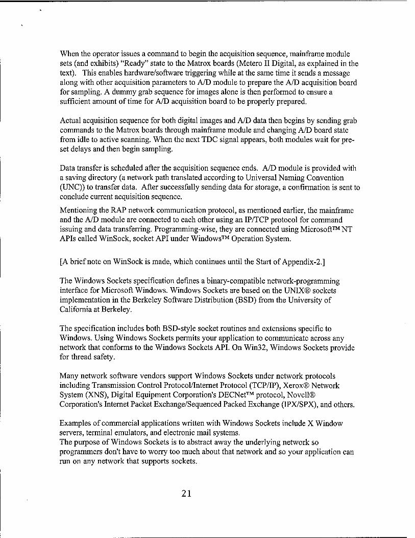
When the operator issues a command to begin the acquisition sequence, mainframe module sets (and exhibits) "Ready" state to the Matrox boards (Metero II Digital, as explained in the text). This enables hardware/software triggering while at the same time it sends a message along with other acquisition parameters to A/D module to prepare the A/D acquisition board for sampling. A dummy grab sequence for images alone is then performed to ensure a sufficient amount of time for A/D acquisition board to be properly prepared.
Actual acquisition sequence for both digital images and A/D data then begins by sending grab commands to the Matrox boards through mainframe module and changing A/D board state from idle to active scanning. When the next TDC signal appears, both modules wait for pre- set delays and then begin sampling.
Data transfer is scheduled after the acquisition sequence ends. A/D module is provided with a saving directory (a network path translated according to Universal Naming Convention (UNC)) to transfer data. After successfully sending data for storage, a confirmation is sent to conclude current acquisition sequence.
Mentioning the RAP network communication protocol, as mentioned earlier, the mainframe and the A/D module are connected to each other using an IP/TCP protocol for command issuing and data transferring. Programming-wise, they are connected using Microsoft™ NT APIs called WinSock, socket API under Windows™ Operation System.
[A brief note on WinSock is made, which continues until the Start of Appendix-2.]
The Windows Sockets specification defines a binary-compatible network-programming interface for Microsoft Windows. Windows Sockets are based on the UNIX® sockets implementation in the Berkeley Software Distribution (BSD) from the University of California at Berkeley.
The specification includes both BSD-style socket routines and extensions specific to Windows. Using Windows Sockets permits your application to communicate across any network that conforms to the Windows Sockets API. On Win32, Windows Sockets provide for thread safety.
Many network software vendors support Windows Sockets under network protocols including Transmission Control Protocol/Internet Protocol (TCP/IP), Xerox® Network System (XNS), Digital Equipment Corporation's DECNet™ protocol, Novell® Corporation's Internet Packet Exchange/Sequenced Packed Exchange (IPX/SPX), and others.
Examples of commercial applications written with Windows Sockets include X Window servers, terminal emulators, and electronic mail systems. The purpose of Windows Sockets is to abstract away the underlying network so programmers don't have to worry too much about that network and so your application can run on any network that supports sockets.
21

The Microsoft Foundation Class Library (MFC) supports programming with the Windows Sockets API by supplying two basic classes. One of these classes, CSocket, provides a high level of abstraction to simplify network communications programming. For more information about MFC socket supports, please refer to "Visual C++ MFC Programming documents" for details.
The Windows Sockets specification, Windows Sockets: An Open Interface for Network Computing Under Microsoft Windows, now at version 1.1, was developed as an open networking standard by a large group of individuals and corporations in the TCP/IP community and is freely available for use. The sockets programming model supports one "communication domain" currently, using the Internet Protocol Suite. The specification is available in the Win32 SDK. Note that a socket is a communication endpoint — an object through which a Windows Sockets application sends or receives packets of data across a network. A socket has a type and is associated with a running process, and it may have a name. Currently, sockets generally exchange data only with other sockets in the same "communication domain," which uses the Internet Protocol Suite. Both kinds of sockets are bi-directional: they are data flows that can be communicated in both directions simultaneously (full duplex). Sockets are highly useful in at least three communications contexts:
• Client/Server models • Peer-to-peer scenarios, such as chat applications • Making remote procedure calls (RPC) by having the receiving application interpret a
message as a function call
However simple Socket is, it doesn't provide enough functionality for End-To-End Programming like the situation we have in the RAP program. We have to derive higher level APIs for ourselves.
We therefore employ the Client/Server Model: contract to the names, A/D module (the Slave Computer) is actually running the Server side, and Mainframe is running the Client side. Why not the other way? The concern here is that in the server side, there ought to be a one to multiple connections, and therefore be active for a certain period of time. And the client just need to ask the server to seek for a connection, if the server fails the request, the client will return to run on its own. If we let the Mainframe be the server, we have to keep it listening on its socket for some time, which can increase the burden on information processing. However, once the connection is established, the end to end connection is two- way (full duplex) and allows data flows in either direction: mainframe program can issue commands to A/D module and module can send A/D data to mainframe program.
Mentioning API for networking in RAP program, we discussed above, we will have to derive our own encapsulation of socket APIs. As discussed, A/D module is running the server side, what it actually does is to open a communication channel and keep "listening" on it, and if the incoming call is acceptable, assign an ID to it. On the other hand, RAP
22

mainframe is running the client side, it will have to actively connect to the server, ask for permission to connect, once accepted, the rest is to exchange information with the server.
In programming language, the A/D module will keep a LISTENING SOCKET to open communication channel; when it accepts a client, it will keep a CLIENT SOCKET to identify the incoming client. On the client side, it will need a MESSAGE SOCKET to send different messages. All these SOCKETS are derived from WinSock APIs. Some basic communication functions are ready for programmers to use.
To simplify the programming situation, only the basic architecture of sockets involved in the program and some useful functions are discussed below:
From the above figure, we can see that each module consists of a View-Document structure. View is the interface that the program reacts with the user: taking keyboard or mouse inputs and display relative information on the screen. Document is the documentation of parameters, and in our case, also sockets.
RAP mainframe computer takes user inputs, some of which were redirected through sockets, and then become the inputs of the A/D module. So, inputs to the mainframe computer are the sole and only command source.
User
RAP Mainframe Experiment
Experiment
Experiment
Message
A/D
A/D View: directlv
t A/D
Client Socket
As an example of Application Programming Interface (API) the following is explained.
CAsyncSocket:: Connect
BOOL Connect( LPCTSTR IpszHostAddress, UINT nHostPort ^/lpszHostAddress: The network address of the socket to which this object is connected: a machine name such as "www.rutgers.edu", or a dotted number such as "128.6.4.5".
23

nHostPort: The port or communication channel identifying the socket application.
A/D module is always running the server side of the communication, and is always "listening" on the channel. So, it is up to RAP mainframe computer to connect to it at its network address at a predefined channel. So, this connect function is used by RAP mainframe computer to connect to A/D module when a connection request is issued by the user.
Both A/D module and RAP mainframe are running DHCP on them. Actual IP address may not be consistent but machine name are always unchanged. According to computer server of Engineering Building that runs the RU2000net, the machine name of RAP mainframe is "shull.engr.rutgers.edu" and that of A/D module is "shul2.engr.rutgers.edu". So when mainframe computer is trying to connect to A/D module, "shul2.engr.rutgers.edu" should be used. Also, communication channel "0" is predefined, which internally is port 700.
CExpDoc: :SendMsg(CString& msg)
CRAP_ADDoc: :SendMsg(CString& msg)
msg: Messages need to be sent. When RAP mainframe or A/D module needs to send a certain message, either to issue command or to confirm operation, the corresponding function is used. In order to trigger certain predefined operations, the following messages are used. Messages sent from RAP mainframe to A/D begin with "RAP_Phase" and are followed by phase ID. Message sent from A/D to RAP mainframe begin with Phase and are followed by Alphabets to classify phase. These messages are listed in Table A-l and Table A-2.
In addition to the predefined messages, A/D and RAP mainframe programs are equipped with Direct Messaging Mechanism, which enables each module to send messages in "Plain English" like: "A/D has received experimental parameters", "Sampling data failed at cycle 2, point 500", etc.
Such Direct Messages are handled by the View-interfaces of each module and are usually put to the monitor for user information.
Phase ID Information RAP Phase 1: Connection establishment RAP Phase2: Experimental parameter transfer RAP Phase3: Trigger of transferring experimental data RAP Phase4: Trigger of preview P/T data RAP Phase5: Set A/D background scanning ON RAP Phase6: Set A/D background scanning OFF RAP Phase7: Send mainframe program executing directory
24

RAP Phase8: Trigger of buffer allocation and background scanning for sample data in A/D. This message is followed by number of cycles to take sample.(<10)
RAP_Phase9: | Trigger of transferring Sample Data
Table A-l: Messages Sent from RAP Mainframe to A/D.
Phase ID Information Phase A: Experimental data transferring completed. Phase B: Preparation of sampling data completed Phase C: Sample data transferring completed Phase D: Preview data transferring completed Phase E: Sampling data Failed Phase F: Parameter transfer OK
Table A-2: Messages Sent from A/D to RAP Mainframe.
RAP
(1) User Prompt for
(5) Turn On A/D signal
Timer
(6) Turn Off A/D signal
(7) Ask for samole data
(12) Display Sample
(13a) Display Samole
(13b) Display Error Messaee
(2) RAP_Phase8 +
(4) Phase B
'► Sampling
(12a) Phase C
(12b) Phase E
A/D
(3) Allocation Buffer and put on scanning
(10a) Wait &
25

Above shows, "Messages Exchange between RAP Mainframe and A/D Module".
Note that during the process of sampling A/D data, the handshake mechanism is illustrated. (Assuming connection has been established and parameters have been transferred):
Appendix-2. Artificial Intelligence Four-color Method (AIFCM)
A-2-1. Four-dimensional Spectrometric Method Setup
As explained earlier in the text, the general scenario of multiple dimension spectrometric methods is to measure radiation at multiple wavelengths from the same source. The spectral data are, then, processed using governing equations set up using radiation models (e.g., mostly rigorous physics laws as shown later) at these wavelengths in order to formulate relations between radiation intensities and species concentrations, mixture and surface temperature, etc.
The space formed by these sought entities is called the variable space (or unknown space). Using Rutgers Super Imaging System (SIS), four geometrically identical infrared images are obtained at four infrared wavelengths, namely 3.8 urn, 3.45 um, 2.47 (im and 2.2 um. These images reflect the radiation intensities at those corresponding wavelengths after being calibrated with the system.
An assumption is then made, according to experimental data from NASA IR Handbook, that at those four specific wavelengths, only combustion chamber wall, water (H20) and soot are the contributing radiation sources. By Single Line Group (SLG) radiation model, governing equations at these specific wavelengths are generated as follows,
Al, =£wanh,X:\Twaii) + £x.Hlo+Soot\-h,\i \Tgas)~ewallh,X,A^wa//)J »Z=l>2,3,4 (A-l)
where, / is the composite intensity at wavelength X^
I (T) is the blackbody intensity at temperature T and wavelength X[:
£x,,source *s me emissivity from radiation source at wavelength Xf, it is evaluated in combined with other parameters such as substance concentration, radiation source temperature T, etc.
Relation Eq. A-l is rewritten to produce the following relation,
h, = /(T^T^iwaterUsoot^P^e^), 1=1,2,3,4 (A-2)
26
where, A,- is predefined and P (pressure), L (path length) and e^u (combustion chamber wall emissivity) can be determined by measurement and/or calculation, so relation (Eq. A-2) can be rewritten as
h., = fW^„(Tgas,Twall,[water],[soot]), »=1,2,3,4 (A-3)
Equation A-3 demonstrates a relation between the vector {Ix }, which is measured and
known and the vector \T ,TwaU,[ water], [soot]}, the unknown variables, both of which are of
degree 4.
Details in SLG model as well as NASA data had been extensively discussed in the master dissertation of Fang Tiegang and the doctorate dissertation of Jansons Marcis at Rutgers.
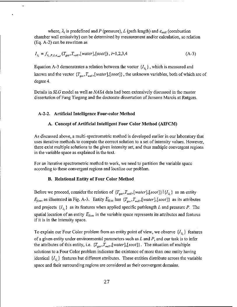
A-2-2. Artificial Intelligence Four-color Method
A. Concept of Artificial Intelligent Four Color Method (AIFCM)
As discussed above, a multi-spectrometric method is developed earlier in our laboratory that uses iterative methods to compute the correct solution to a set of intensity values. However, there exist multiple solutions to the given intensity set, and thus multiple convergent regions in the variable space as explained in the text.
For an iterative spectrometric method to work, we need to partition the variable space according to these convergent regions and localize our problem.
B. Relational Entity of Four Color Method
Before we proceed, consider the relation of {Tgas,Twall,[water],[soot]} I {Ix } as an entity
Efcm, as illustrated in Fig. A-3. Entity Efcm has {T ,Twal„[water],[soot]} as its attributes
and projects {Ix } as its features when applied specific pathlength L and pressure P. The
spatial location of an entity EfCm in the variable space represents its attributes and features if it is in the intensity space.
To explain our Four Color problem from an entity point of view, we observe {Ix } features
of a given entity under environmental parameters such as L and P, and our task is to infer the attributes of this entity, i.e. {Tgas,Twa„, [water], [soot]}. The situation of multiple
solutions to a Four Color problem indicates the existence of more than one entity having
identical {Ix.} features but different attributes. These entities distribute across the variable
space and their surrounding regions are considered as their convergent domains.
27

® Attribu O Featur
Fig. A-3: Four Color Relation Entity
Partition the Variable Space
According to previous discussion, the variable space could be viewed as a space made up of several sub-spaces, each of which is a convergent domain for one of the multiple solutions. The key to localize our problem is to partition our variable space into convergent domains according to these possible solutions.
Recall in computational geometry, the resulted partitioned 2D geographic domain of the postal office problem is also made up of sub-domains according to the available sites. To draw an analogy between our problem and the postal office problem, our solutions can be considered as "sites" to the variable space, as the "postal offices" to a geographical domain; the convergent space for individual solution is equivalent to partitioned postal area according to postal offices. Fig. A-4 gives an example of postal office problem applied in predicting trading areas in Netherlands, which gives an example of subdivision situation for a Four Color problem where Sj, z-0,1, 2.. .3 are the possible solutions.
capitals
Fig. A-4. The trading areas of the capitals of the twelve provinces in the Netherlands, as predicted by the Voronoi assignment model [4]
28
1.2E-05
2.0E-06
I.OE+00
1050 1250 1450 1650 1850 2050 2250 2450 2650
Tgas(K)
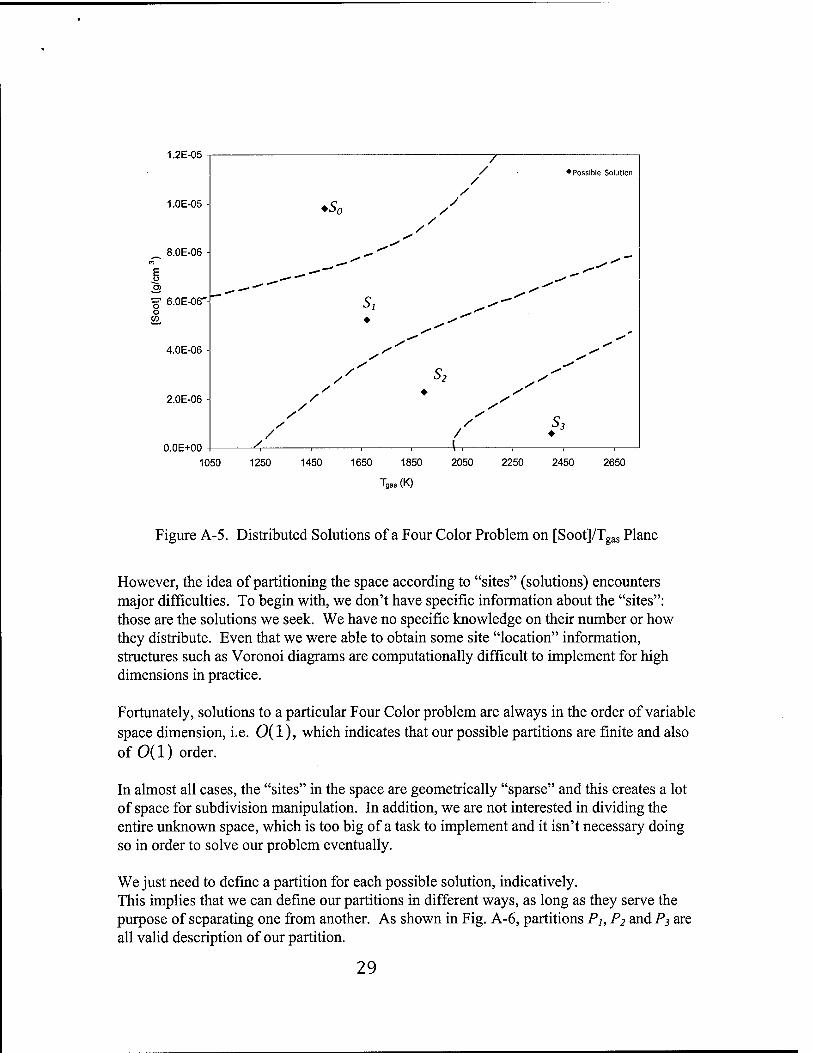
Figure A-5. Distributed Solutions of a Four Color Problem on [Soot]/Tgas Plane
However, the idea of partitioning the space according to "sites" (solutions) encounters major difficulties. To begin with, we don't have specific information about the "sites": those are the solutions we seek. We have no specific knowledge on their number or how they distribute. Even that we were able to obtain some site "location" information, structures such as Voronoi diagrams are computationally difficult to implement for high dimensions in practice.
Fortunately, solutions to a particular Four Color problem are always in the order of variable space dimension, i.e. 0(1), which indicates that our possible partitions are finite and also of 0(1) order.
In almost all cases, the "sites" in the space are geometrically "sparse" and this creates a lot of space for subdivision manipulation. In addition, we are not interested in dividing the entire unknown space, which is too big of a task to implement and it isn't necessary doing so in order to solve our problem eventually.
We just need to define a partition for each possible solution, indicatively. This implies that we can define our partitions in different ways, as long as they serve the purpose of separating one from another. As shown in Fig. A-6, partitions Pj, P2 and P3 are all valid description of our partition.
29

1.2E-05
1.0E-05
8.0E-06
E
S 6.0E-06
o o w
4.0E-06
2.0E-06
O.OE+00
/ /
/ C / »Possible Solution
■J0 s ♦ / /
Pi ^
^-^>^*2\ ^ ~
/ n^^ / / ^^ / '
' , , , V , , ,— 1050 1250 1450 1650 1850 2050 2250 2450 2650
Tgas(K)
Figure A-6: Different Forms of Partitions
Therefore, we do not need the exact site information in order to obtain partitions of the variable space. If we are able to obtain some samples from each of these partitions, preferably close to the solution site in the variable space, e.g. in Fig. A-6, nh i=l,...,5 are the samples from 5^ partition, we in turn can describe each partition using these samples, call them "close matches".
A four-dimensional convex hull formed by close matches from a particular partition typically encloses a sub-space of such a partition.
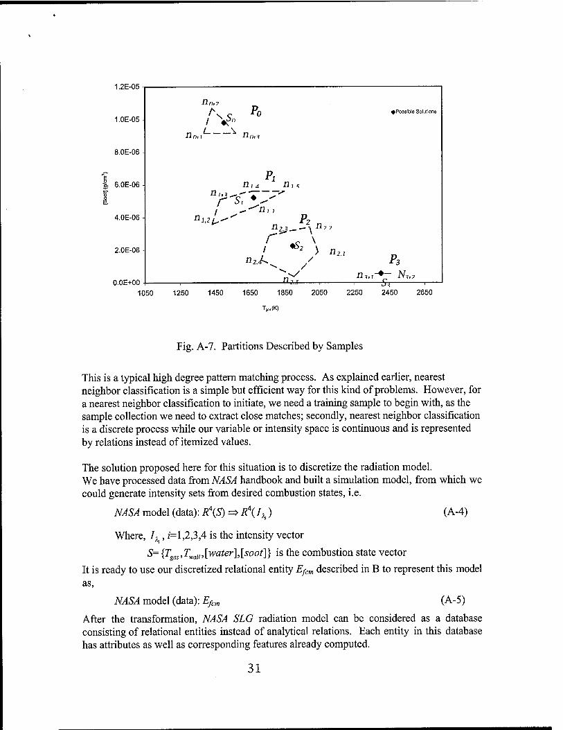
Applying this concept to the variable space w.r.t individual possible solution and we therefore "partition" the entire variable space. An example is given Fig. A-7.
To summarize, in order to localize our Four Color problem, we need to partition the variable space according to solutions. Without specific knowledge on the solutions, we turn to close matches of these solutions to form individual partitions instead.
Proposition of Artificial Intelligent Four Color Method As discussed in 0, the task of localizing the Four Color problem is reduced to finding close matches for possible solutions from each partition. Since only the {Ix } features of these possible solutions are available, finding their close matches can only be done through matching patterns in {Ix } features.
30
1.2E-05
1.0E-05
8.0E-06
•g. 6.0E-06
4.0E-06
2.0E-06 •
O.OE+00
Tin,? ♦Possible Solutions
n L \ „ 11 n, i Un,i
Pi n1d n,s
23 ,,, . —- >*
r s, ♦ ^ ^/-^ P2 „
n2j-.-\n??
n2.^ / P3 "-» / ^^ ii?,»-♦- N?l7
-I , , , ^A^—i i JJ
1050 1250 1450 1650 1850 2050 2250 2450 2650
T,„(K)
Fig. A-7. Partitions Described by Samples
This is a typical high degree pattern matching process. As explained earlier, nearest neighbor classification is a simple but efficient way for this kind of problems. However, for a nearest neighbor classification to initiate, we need a training sample to begin with, as the sample collection we need to extract close matches; secondly, nearest neighbor classification is a discrete process while our variable or intensity space is continuous and is represented by relations instead of itemized values.
The solution proposed here for this situation is to discretize the radiation model. We have processed data from NASA handbook and built a simulation model, from which we could generate intensity sets from desired combustion states, i.e.
NASA model (data): R\S) => R\ 1^) (A-4)
Where, /, , z'=l,2,3,4 is the intensity vector
S= {Tgas,Twall,[water],[soot]} is the combustion state vector
It is ready to use our discretized relational entity E/cm described in B to represent this model as,
NASA model (data): Efcm (A-5)
After the transformation, NASA SLG radiation model can be considered as a database consisting of relational entities instead of analytical relations. Each entity in this database has attributes as well as corresponding features already computed.
31
The transformation of the radiation mode provides us with a pre-computed database, which can be considered "experienced" data with proven credibility and thus provides a working environment for nearest neighbor classification.
Eqs. (A-4) and (A-5) demonstrate representation of NASA SLG radiation model by data instead of analytical equations as specified in 1.1. Now that we have a ready-to-use database for a nearest neighbor classification process to retrieve close matches to the given
entity's {Ix } feature.
This is a supervised non-parametric pattern classification, where the pattern refers to the
{Ix } features. Note that this pattern classification we adopt differs from an usual nearest
neighbor classification in that we will preserve all possible nearest neighbors that meet the closeness criterion or the similarity function instead of just choosing the very nearest.
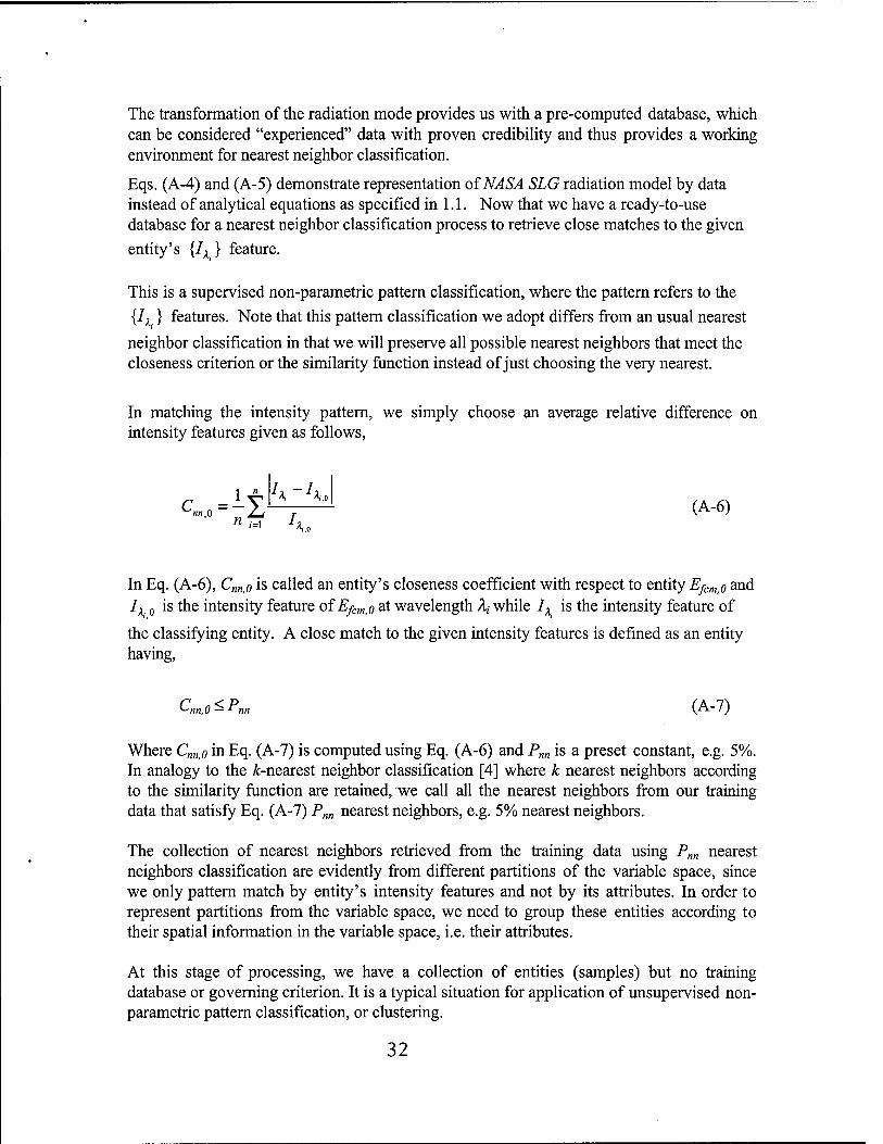
In matching the intensity pattern, we simply choose an average relative difference on intensity features given as follows,
1 X1
C ^ ^i ^i,0 1 x~> "i '
(A-6)
In Eq. (A-6), Cmo is called an entity's closeness coefficient with respect to entity Efcnii0 and 1^ 0 is the intensity feature of Efcm0 at wavelength A,- while 1^ is the intensity feature of
the classifying entity. A close match to the given intensity features is defined as an entity having,
Cnn,o<Pm (A-7)
Where Cm0 in Eq. (A-7) is computed using Eq. (A-6) and Pnn is a preset constant, e.g. 5%. In analogy to the ^-nearest neighbor classification [4] where k nearest neighbors according to the similarity function are retained, we call all the nearest neighbors from our training data that satisfy Eq. (A-7) Pnn nearest neighbors, e.g. 5% nearest neighbors.
The collection of nearest neighbors retrieved from the training data using Pm nearest neighbors classification are evidently from different partitions of the variable space, since we only pattern match by entity's intensity features and not by its attributes. In order to represent partitions from the variable space, we need to group these entities according to their spatial information in the variable space, i.e. their attributes.
At this stage of processing, we have a collection of entities (samples) but no training database or governing criterion. It is a typical situation for application of unsupervised non- parametric pattern classification, or clustering.
32
Appropriate inter-cluster distances are then chosen in combination with the attribute grids when we discretize NASA SLG model to create our training database. The resulted nearest entities are classified against each other on the patterns possessed by their attributes.
Using these inter-cluster distances, we cluster nearest entities into smaller groups, each of which projects similar patterns on their attributes. Entities within each cluster are then further process to produce a substantial subset that is the compact version of such a cluster. Redundant entities are discarded. For each of these resulted clusters, a representative entity is computed by averaging individual attribute of entities contained in the cluster. Attributes of the cluster can then be approximated by this entity.
To a given Four Color problem, there is one and only one legitimate solution. It is clear that all but one of these clusters contains false information of a true solution and should be eliminated. This is a pattern discriminate analysis. Since the representative entity of each cluster projects similar patterns to all entities within the cluster as well as the solution contained within the cluster, it is safe to perform pattern discrimination on the representative entity before an exact solution becomes available.
Hence, all computed representative entities are given an assessment on validity within the actual experiment scenario. A coefficient is computed for each representative entity to indicate relative validity within the particular experiment conditions. The one with highest value of validity coefficient is considered most likely to produce a more precise solution to the Four Color problem we have discussed so far. Such a cluster is preserved for further processing while the rest are discarded.
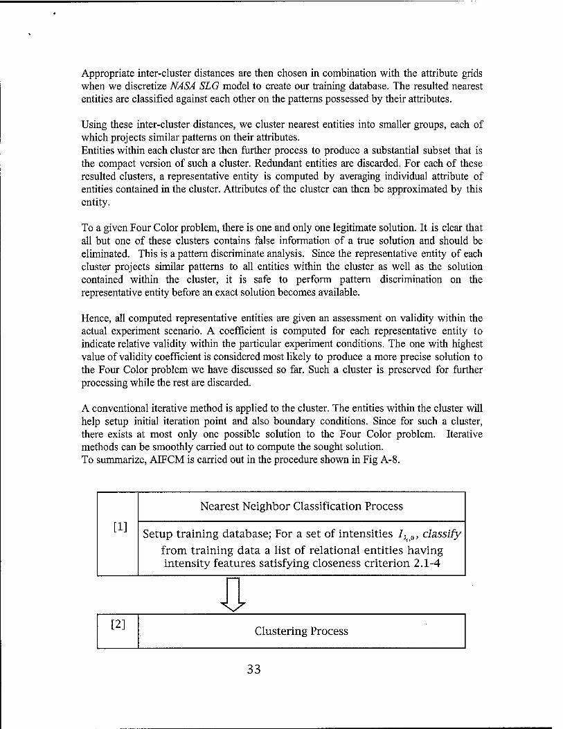
A conventional iterative method is applied to the cluster. The entities within the cluster will help setup initial iteration point and also boundary conditions. Since for such a cluster, there exists at most only one possible solution to the Four Color problem. Iterative methods can be smoothly carried out to compute the sought solution. To summarize, AIFCM is carried out in the procedure shown in Fig A-8.
[1]
Nearest Neighbor Classification Process
Setup training database; For a set of intensities I^fi, classify
from training data a list of relational entities having intensity features satisfying closeness criterion 2.1-4
33

Perform clustering analysis on entities resulted from [1] to form clusters of entities having similar attribute patterns;
Produce attribute entity for each cluster
Discriminating Process
Use attribute entity from [2], combined with actual experimental conditions, assess validity on each entity cluster; preserve only the cluster with highest validity
coefficient
V
[4]
Solving Process
Form localized domain for the cluster resulted from [3], solve for solution using a conventional iterative method
Figure A-8: AIFCM Proposed Procedure
Appendix- 3. Stability Analysis using Vector Defined Characteristics
The need and concept of the new flame-stability-analysis method is discussed in detail below. At first, a new property of space-resolved flame propagation is defined and justified of its usefulness. Case study and analysis are also explained.
A-3-1. Characteristic Vector Set in Continuous Form
For each point P(x,y) in a continuous and connected two-dimensional area A with a planar function f(x,y) defined on A, define characteristic vector for point P as:
VP = f(x, y)-(x + y) = f(x, y) ■ (xi + yj), where P (x,y)eA
In the above representation,/^, v,) is also called the weight or strength of the vector. The characteristic vector for area A is defined as,
34

- \vp-dA V — ^A — -A 'A ~
jjf(x> y) • tß+y])dxdy
\dA jjdxdy
Normalize VA using the function mean, i.e. assign function mean as the vector weight,
\\f(x, y)dxdy jjf(x, y) ■ (xi + yj)dxdy jjf(x, y) ■ (xi + yj)dxdy VA=^L
\\dxdy jjf(x,y)dxdy jjf(x,y)dxdy _ A
VA is then represented by vector
\\dxdy A
\\f(x,y)(xi + yj)dxdy _A
\\f(x,y)-dxdy
jjf(x,y)dxdy
\\f(x,y)dxdy with a scalar ——j-.
II dxdy
(expected function value) as the vector weight.
Figure A-9: Representation of A
As discussed above and illustrated in Fig. A-9, VA has weight of mean function value
jjf(x> y)dxdy jjf(x> y) ■ (xi + yJ)dxdy - and xH+y] = -A
jlJxt/y \\f(x,y)dxdy
35
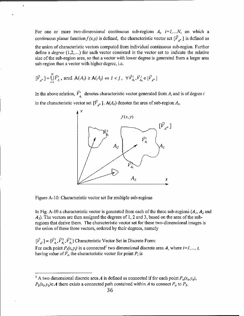
For one or more two-dimensional continuous sub-regions Au i=l,...N, on which a
continuous planar function/(x,y) is defined, the characteristic vector set [V N ] is defined as
the union of characteristic vectors computed from individual continuous sub-region. Further define a degree (1,2,...) for each vector consisted in the vector set to indicate the relative size of the sub-region area, so that a vector with lower degree is generated from a larger area sub-region than a vector with higher degree, i.e.
[VA = Un , and A(A} > A(Aj) ^ i <j, yf'VU[VAri] 1=1
In the above relation, V' denotes characteristic vector generated from^,- and is of degree i
in the characteristic vector set [V „ ]. A(Ak) denotes the area of sub-region Ak.
k Y f(x,y)
Ix2 f [^»]
T2 I n ^j-J A2
■ly \il
V- A3 X
Figure A-10: Characteristic vector set for multiple sub-regions
In Fig. A-10 a characteristic vector is generated from each of the three sub-regions {Au A2 and As). The vectors are then assigned the degrees of 1,2 and 3, based on the area of the sub- regions that derive them. The characteristic vector set for these two-dimensional images is the union of these three vectors, ordered by their degrees, namely
[VA3 ] = {V\x, V2h, V\} Characteristic Vector Set in Discrete Form:
For each point Pi(xby^ in a connected1 two dimensional discrete area A, where i=l,.... t, having value of Ft, the characteristic vector for point Pt is
1 A two dimensional discrete area .4 is defined as connected if for each point Pa(xa,ya), Pb(xb,yb)eA there exists a connected path contained within A to connect Pa to Pt,.
36

Vt = Ft(xJ + yj), where Pt=(xby} eA
And the characteristic vector for area A is defined as,
t/t S^i ttw + yJ) V =-£=1 = -i=L_ 1=1 F E^(^+j,7)
J J=l
X*. 1=1 1=1
f
Z*. 1=1
Note that VA is also normalized by mean value, X^ X^(^+x7) i=i , and 1=1 is the
2", i=i
representing vector for VA . The characteristic vector set for one or more two-dimensional connected sub-regions is defined in the similar way as the continuous form: as the union of characteristic vector computed from individual connected sub-regions. Also assign each vector a degree based on the number of points consisted in the sub-region from which the characteristic vector is computed.
As discussed earlier, we need to account for two main factors in spatial images: geometric difference and intensity difference. Our proposed characteristic vector set is capable of signifying such differences because it uses a weighted vector transformation and generation. The weight of the vector indicates the overall intensity of the examined area while the vector position indicates the area geometry.
A-3-2. CaseStudy-I
As discussed in 4.3, for a 2D intensity profile, Characteristic Vector of degree 1 in the Characteristic Vector Set (CVS) indicates the geometric position as well as intensity feature of the most dominant area of the overall profile. Since the infrared images acquired using RSIS are 2D intensity profiles in time scale (frames), by examining characteristic vectors of degree 1 for each frame, we can trace how such "hot spots" propagate as well as their travel speed. The example demonstrated thereby is to compare the propagation of "hot spots" in engine equipped with different intake regulatory plates, as shown in Fig. A-l 1.
Experiments are run on a gasoline engine equipped with different intake regulators. Characteristic Vector of degree 1 is computed for each experiment and compared with each other. Figure A-12 demonstrates the geometric trace of the "hot spot" configured by the Characteristic Vector of degree 1. It shows that the experiment using Quarter Plate intake regulator demonstrates a most pronounced travel trace across the entire combustion chamber.
37

Figure A-l 1: Intake Regulators (Shaded Area Indicates Plate)
(a) Original (b); Half Plate Half Hole; (c) Half Plate (d) Quarter Hole
50
30
Quarter Plate
Half Plate Half Hole
X Original
20 30 40
Fig. A-12. Trace of Characteristic Vector of Degree 1.
It shows that using any intake regulator increases the maximum intensity as well as the rate of increasing intensity.
38

2500'
1500
1000
500
Intensity Half Plate Half Hole
-40 CA
Fig. A-13. Intensity Evolution of Characteristic Vector of Degree 1
Application of Stability Factor. Stability factor discussed earlier is applied to multiple engine cycles for different experimental setup, such as different fuels, different engine spark ignition timing, etc, to compare engine performance.
The following example compares stability on engine cold start using fuel No. 1 (Sunoco) and fuel No.2 (Texaco).
a. Computation on single Crank Angle, multiple cycles
Gd,0 Ö/.0 Wo) Co Vo Fuel No.
1 11.797 264.885
1154.42 2
50 (0.37, 0.23)
Fuel No. 2
8.171 172.051 715.980 49 (0.26, 0.22)
Table A-3: Stability Factor of degree 1 Sample Calculation Cycle 1-50 (M=50), Wavelength at 2.2um, Sample factorp=5%
Crank Angle: 15 aTDC, D=32
b. Computation on consecutive Crank Angles, multiple cycles
Vo = (Vs.O, V/.o) 7 aTDC 11 aTDC 15 aTDC 19 aTDC 23 aTDC 27 aTDC
Fuel No.l
(0.28,0. 17)
(0.39,0.2 1)
(0.37,0.2 3)
(0.38,0.1 7)
(0.20,0. 13)
(0.24,0. 16)
39

Fuel No.2
(0.23,0. 12)
(0.26,0.1 4)
(0.26,0.2 2)
(0.28,0.2 3)
(0.27,0. 18)
(0.27,0. 19)
Table A-4: Stability Factor of degree 1 vs. Crank Angle Cycle 1-50 (M=50), Wavelength at 2.2\im, Sample factor p=5%, D=32
The above computation indicates that running condition in the experiment using fuel No.2 has
higher spatial stability and comparable intensity stability compared to fuel No.l.
The proposition and application of Characteristic Vector and Stability Factor in engine study are extensions of research projects carried out at Rutgers ICE laboratory using Rutgers Super Imaging System. Both parameters fully utilize the 2-dimensional intensity profiles acquired using RSIS and quantify the geometric variation as well as intensity variation in the statistical analysis of engine operations. Characteristic vectors quantify the spatial distribution of different intensity areas while the proposed stability factor further accounts for cyclic variation in both aspects.
A-3-3. Case Study-II Engine Flame Research
Application Formulation. Intensity profiles acquired using Rutgers Infrared Imaging System can be treated as time series two-dimensional discrete infrared images. Currently, the system is capable of taking infrared images from consecutive engine cycles at multiple wavelengths. Images from one cycle at each wavelength consist of 64 frames, of which the dimension is of 64x64 pixels. Each pixel Pt(x»yd having intensity value of Ifayj) in a frame has the following characteristic vector,
VPt = /(W*)' (*/ + yJ) > 0<^<64, 0<^<64
Examples of point characteristic vectors are given in Fig. A-14.
After this formulation, we are ready to perform analysis using the discrete form of characteristic vector set concepts to extract meaningful information from the intensity profile.
Define: characteristic vector set for an infrared intensity image F as follows, Consider sub-region(s) Sp of F, such that area of Sp, A(Sp) and area of F, A(F) satisfy A(Sp) = p ■ A(F), where p is a percentage called sample factor
And intensity values in Sp are higher than those in the region in F other than Sp, i.e. I(xm>yJ>I(xq,yq). for any m(xm,yje Sp, and any q(xq,yq)e (F/Sp)1
' (F/Sp) denotes area in F but not in Sp. The relation can be alternatively expressed as
For any m(xm,yJeSp, -n3 q(xq,yq)e (F/Sp), such that I(xm,yJ<I(xq,yg)
40

^=1723-(171+40./)
F5=2019-(51/+20y)
17 51
Fig. A-14. Formulation of Point Characteristic Vector
p f Intensity
HI
Fig. A-15. Derivation of Sp in 3D perspective,
(a) Image F in 3D view (b) Sp is chosen by choosing a percentage/? of the most active area.
Derivation of Sp is given in three-dimensional perspective, where an additional dimension is assigned to intensity values. As discussed earlier, p-5% and A(SP) = 64x64x5% = 205 pixels.
Cluster sub-region Sp into sub-divisions Dij}, z'=l,...,n, such that each Dip is inner connected, define characteristic vector set for F at sample factor p as the vector set of characteristic vector computed from Dips
41
^;]=u^„ J=I
where p is the sample factor, n is the dimension of the vector set and i is the degree of individual
characteristic vector as defined above. Note that VI is the before defined discrete form of area i.p
characteristic vector except for an additional sample factor p. Call V'D characteristic vector of
degree i at sample factor/?.
An example on generation of characteristic vector set from the infrared images is given in Figure 5, where an original intensity profile is shown in (a). A sample factor p=5% is applied to (a); only the 5% of most intense pixels are retained as Sp, shown in (b).
The resulted image sections after factor-sampling are then clustered into connected sub-divisions, namely D5o/oJ and D5%: 2 as in (c). Characteristic vectors are finally computed from individual sub- divisions to produce VX
D o and V% t using the above discussed method.
Characteristic Vector Set and Stability Factor for a group of images. The new Rutgers Infrared Imaging System is capable of taking infrared images on consecutive engine running cycles.
This capability has opened up opportunities for engine research from different aspects. An important new direction is to investigate engine operation stability from spatial intensity profiles instead of old-fashioned single point pressure time series.
For a group of M images having similar engine combustion conditions (e.g. engine setup, crank angle), Flt_iM, choose a sample factor p and compute characteristic vector set [Vp"]kfov each image Fk, k=l,...,M, where n^ is the vector set dimension for image Fk.
Choose a cut-off degree dc, and compute the union of vectors having degree i< mm(nk,dc), i.e.
WpM4 1 = U W'p\, whereN= mm(nhdc)
An example of [VpMid ] computation for a group of images is given earlier where each point in the
figure represents the end point position of a characteristic vector while the weight of the vector is omitted at this moment.
42

Fig. A-16. Generation of Characteristic Vector Set
(a) Original Image (64x64) (b) Image after trimmed by sample factor p=5% (c) Cluster Image into sub-divisions (d) Compute vectors for individual sub-division
Without being discriminated in vector degrees, all vectors in [VpMd ] are clustered into
vector groups using an inter-cluster Euclidean distance,
[Vn«]m,m=l,...,N
where N is the number of vector groups after clustering and nm is the number of vectors in group m, also called dimension.
Sort these groups by descending dimensions, so that,
[VnJ\, i=l,...,N and nt> n}- for i<j
43

60
50
O degree 1
D degree 2
A degree 3
40 fr
Y
30 <af°
20- &
10-
0
°ff&>o
/£A
10 20 30 40 50 60
Fig. A-17: Computation of [VpMA ], CA = 28 degree aTDC,;?=5%, wavelength = 3.8um, 9
consecutive cycles (M=9), dc = 2
The result of clustered vector sets for \VpMd ]is given earlier.
Compute deviation on inner-cluster Euclidean distance ad:i and mean intensity Eflj) and intensity deviation ajy for group i,i=l, ...,N Define: Stability Factor of degree i for a group of M images v,
ct D E(I,)
where od:i is standard deviation on Euclidean distance for vector group /, GJJ is standard deviation on mean intensity E(IJ are computed on vector group /, Ci is number of distinct images contributed to the computation of vector group i,
I,i
E{It) is called the coefficient of variance on intensity for vector group i,
D is a constant representing image geometry used to normalize Gdti, an usual choice
is —-, where Lc is image geometric characteristic length. For our application, J^ =
64, soD= 32.
44

60
50 -
40
30
20
10
O degree 1
D degree 2
L'5%J3 A degree 3
%
- ^ W?%\
- © WsVeU
1/5% J2 &£ K%]5
x-, .-s' 1 1 1 1
10 20 30
X
40 50 60
Fig. A-18: Cluster [VpMA ] CA = 28 degree aTDC/^5%, wavelength = 3.8um, 9 Consecutive cycles (M=9), dc=3.
M The introduction of — is to compensate for the penalty on irregularity missing from
the computation of —- and D £(/,)
Fig. A-19 illustrates the computation of stability factors on the studied case.
General guidelines when comparing stability factors are: M <Jd ■
1. First coefficient vc; = ^- represents combustion spatial stability rS,i c, D
M <5r 2. Second coefficient v,. = — represents combustion intensity/reaction ' c,. £(/,.)
stability 3. Smaller factor coefficient represents higher stability.
45

60- O degree 1
D degree 2
50-
$> Ofe. 2,v, 2) = (0.25,0.23)
A degree 3
40-
30- Ä (vs,o,v|,0) = (0.12,0.11) s JA
20- <yS.3,\3) = (0.29,0.33)
10- (VS.1,VI.1) = (0.16,0.16) (vs,4,v||4) = (0.33,0.31)
n-
£&*>),
10 20 30
X
40 SO 60
Fig. A-19: Stability Factors Sample Computation CA = 28 degree aTDC,/?=5%, wavelength = 3.8mm, 9 consecutive cycles
Appendix- 4. HITRAN - Gas Radiation Models
A-4-1. Line-by-Line Gas Radiation Model using HITRAN Database
The jfflgh-Resolution r&4iVsmission (HITRAN) database is a compilation of molecular data maintained by a consortium comprising among others the Air Force Research Laboratory, Harvard-Smithsonian Center for Astrophysics, NASA Langley Research Center and the Jet Propulsion Laboratory [Rothman et al, 1998].
The HITRAN data is a widely recognized standard that has been periodically updated and corrected since publication in 1973 by the Air Force Cambridge Research Laboratories and approved for public release [McClatchkey et al, 1973]. The database contains characteristic parameters of known energy level transitions that may be utilized to produce a line-by-line radiation model.
The 2004 edition of HITRAN contains line data for thirty-nine molecules. Data is available for the different isotopes of each molecule. Although primarily intended for atmospheric studies, also are included important combustion species such as H2 O, C02, CO, NO,
NO 2, OH and the common fuel CH4. Given parameters are theoretical results many of which have been validated or corrected by experiment. HITRAN 2004 contains spectral line information on the molecules shown in Table A-5.
46

Molecule Transitions Molecule Transitions 1 H20 63197 21 HOC1 16276
2 co2 62193 22 N2 120
3 o3 311481 23 HCN 4253
4 N20 47835 24 CH3C1 31119
5 CO 4477 25 H202 100781
6 CH4 251440 26 C2H2 3517
7 o2 6428 27 C2H6
4749
8 NO 102280 28 PH3 11790
9 so2 38853 29 COF2 70601
10 N02 104223 30 SF6 22901
11 NH3 29084 31 H2S 20788
12 HN03 271166 32 HCOOH 24808
13 OH 42373 33 H02 38804
14 HF 107 34 O 2 15 HC1 613 35 C10N02 32199
16 HBr 1293 36 NO + 1206
17 HI 806 37 HOBr 4358 18 CIO 7230 38 C2H4
12978
19 OCS 19920 39 CH3OH 19899
20 H2CO 2702
Table A-5. Molecules For Which Spectral Line Data is Available in HITRAN 2004 (From [Rothman et a 1,2005])
The HITRAN database provides the requisite data for calculation of the absorption coefficient of a particular gaseous species. Table A-6 lists the fields provided by the database for each line or transition.
Symbol Parameter M Molecule number HITRAN assignment I Isotope number Numbered by abundance n Vacuum wavenumber of
transition in cm~l
s Intensity in cm~x 1 {molecule■ cm"2) at 296K
47

A Einstein A-coefficient jn s-
7 ■ 1 air
'self
Air-broadened half-width HWHM at 296K in
cm'11 atm Self-broadened half-width HWHM at 296K in
cm'11 atm £' Lower-state energy -m cm~x
n Temperature-dependence dimensionless, with air
exponent for yair y-air{T)=y'air(T0)x(T01 T)n°'
y . Air pressure-induced line- -m cm-x / atm at 296K shift
y' Upper-state Global quantum number
y" Lower-state Global quantum number
Q ' Upper-state Local quantum number
Q " Lower-state Local quantum number
o' Upper-state statistical weight
p-" Lower-state statistical weight
Table A-6. Data Fields of HITRAN 2004 Database (From [Rothman et a I, 2005])
Radiation Model
Utilizing the molecular parameters on the HITRAN database, a line-by-line radiation model was written in C++ to calculate the emissivity of homogeneous gas mixtures. Both Lorentz and Doppler broadening effects were considered. The high-resolution output of the radiation model was conditioned through various trapezoidal and gaussian instrument functions to predict results observed by a laboratory spectrophotometer and narrow-band filters.
Line-Intensity Correction The line strength or intensity may be calculated from first principles by Equation (l)[Modest, 2003][Ludwig et al, 1973]:
87ZT3 77 |
3 '2| Q(T)T S =mJL\5t J—^(l-e-^,kT)e-E>lkT (A-8)
where:
48

S = line intensity at wavenumber 77,
k= Boltzmann's constant, p= total pressure of the gas volume, T- temperature of the gas volume, Q(T)= the partition function for the particular molecule,
E2 = the lower energy level of the energy transition creating the line S,
i i2
9? I = weighted transition moment for the particular molecule and transition that is related
to the Einstein spontaneous emission coefficient A^2 through:
3« Si
where: g. is the degeneracy of energy level i
The parameters provided by HITRAN (Table 2) are for the reference temperature of 296K. However, the line intensity has a strong explicit temperature dependence as well as an implicit one through the partition function Q(T). The line intensity must be corrected for temperatures other than 296K. Evaluating Equation (1) at the reference temperature and dividing by itself yields a temperature-corrected line intensity, Eq. (A-10).
Sn(T)=S (T jg^W-W [l-exp(M/^)]
The partition function Q{T) required by Equation (3) was calculated using a subroutine developed by Fisher et al [Fischer et al, 2003]. This work is a comprehensive set of total internal partition sums for all of the chemical species whose line data is available in the HITRAN 2000 database. This FORTRAN subroutine was compiled into a dynamic-link library (dll) and called from the C++ code.
Natural Line Broadening Physically emission lines are not of infinitesimal width. Natural Broadening, Collision Broadening, and Doppler Broadening are three known mechanisms of phenomena that distribute the line strength S across wavenumber to produce a wavenumber-dependent absorption coefficient K '.
Sn = jAjiKndV (A-ll)
49

Natural Broadening is an effect resulting from the uncertainty in the exact energy levels E
and E2 of the line transition according to Heisenberg's uncertainty relation:
AE-At>— (A-12) 2K
from which follows [Herzberg, 1950]:
b=—- (A-13) 27TT
where: b= half-width in ergs of an energy state whose lifetime is r • A natural line width is the sum of widths of the upper and lower energy states of a
particular transition and for strong lines is on the order of 0.001 cm'1 [Herzberg, 1950]. The shape of the naturally-broadened line follows the Lorentz distribution [Siegel etal, 1981]:
S b K= "- - (A-14)
n 7C(n-TI0)2+li
where: K = absoption coefficient at wavenumber 77,
770 = center wavenumber of the transition line,
b = half-width for natural broadening.
For engineering applications, natural broadening effects are usually neglected [Ludwig et a\, 1973; Modest, 2003; Siegel etal, 1981].
Collision Line Broadening Molecules are considered to collide when the distance separating the molecules decreases such that inter-molecular forces become significant. When molecules are in this state of collision, their potential energy changes and is different than that of separated molecules. Further, if absorption is taking place during this state of collision, frequencies other than those for widely separated molecules will be absorbed [Herzberg, 1950]. Since there is a continuum of kinetic and potential energies of the molecules colliding, the resultant spectrum is also a continuum. Collision Broadening is often the primary mechanism through which lines are broadened and accounts for the observed effect on the absorption properties of a gas by a second species which may otherwise be transparent. Collision-broadened spectral lines are symmetric about the center wavenumber and are assumed to follow the Lorentz line shape;
S b
' K(7]-r}Qf+tf
where:
50
bc is the collision-broadened half-width derived from kinetic theory [Modest, 2003; Siegel
etal, 1981]:
^=-r-T= (A-16) yJJZ c0yjmkT
where: D= effective diameter of the molecule, p- total gas pressure, m= molecule mass, T= absolute temperature.
Recognizing the temperature and pressure dependence, the parameter b may also be
defined relative to a reference state, b 0:
bc = bc^)\j (A-17)
where: T0 = reference temperature, PQ = reference pressure.
Eq. A-17 illustrates the p I yJT dependence of the half-width and the reason collision broadening is also referred to as Pressure Broadening. While Eq. (A-16) predicts the temperature and pressure dependence of bc, the half-widths
of individual lines in a spectrum are different, and in a mixture the broadening powers of each component species must be considered separately[Ludwig et al, 1973]. The general expression for the half-width of a spectral line in a mixture can be written:
ba=lbc0iJPj = dbco^j)P (A-18) j j
where: y = collision-broadened line half-width of species i, p= total pressure of the mixture,
c. = the concentration of species j, p.= partial pressure of species j, bco = the line half-
width of species / broadened by species j at unit pressure.
The effect due to the term bco , i=j is known as self-broadening and is due to an
emitting/absorbing molecule colliding with another molecule of the same species. There are two types of self-broadening collisions: non-resonant and resonant. The latter type is due to a collision of two molecules having large permanent electric dipole moments that are in neighboring rotational states. These resonant collisions interact strongly and must be considered for polar molecules such as H2 O, but do not exist for symmetric molecules such
as C02 [Ludwig et al, 1973]. The collision half-width may then be represented as being
proportional to: ba = baaPa
+ babPb (A-19)
51

where the subscripts a and b designate the contributions to the half width by self and foreign gas broadening. Introducing the temperature dependence shown in Eq. A-17 the effect of both resonant and non-resonant collisions are considered:
*>a=(L (ba,j\ Pj (y)"'J ]+(*Jo P &"'■' (A-20) J
where: ba= collision-broadened half-width of radiating species i, ba .= collision line width
parameter of foreign gas j broadening the radiating species i at reference temperature T0,
p. = partial pressure of species j, n. .= foreign species half-width temperature correction
factor, ba. = collision line width parameter for self-broadening at reference temperature TQ,
p. = partial pressure of species i, n.. = self-broadened half-width temperature correction factor.
In this formulation, the non-resonant collisions between like molecules are included in the summation of foreign gas broadeners (i=j), and the resonant collisions in the separate term. Each term is allowed a separate temperature dependence.
When a mixture of gaseous species is considered, an effective pressure is used to replace the total pressure in A-14 to account for the collisions between the non-radiating species in the mixture.
Because HITRAN data is predominantly used for atmospheric modeling, the database provides a collision line-width parameter weighted for the component species of the atmosphere, bCair, in addition to the self-broadening parameter ba. These parameters are provided for every transition line. For the spectral properties of a single component in air, the collision half-width was calculated using Eq. A-21.
ba(T^<hm(b ip.J^^-p^+b^ipMp^) (A-21)
where the reference temperature and pressure TQ, P0 are 296K and 1 atmosphere, respectively.
For mixtures for which broadening effects from components other than air and self- broadening are to be considered, broadening coefficients are taken from the literature. Line- by-line values are often not available and average values of these coefficients are often used.
52

Doppier Line Broadening
The frequency of a wave emitted by a moving source will to an observer appear modified
according to the Doppler shift:
7?=770(1+-) (A-22) c
where:
r\0 = the frequency of the wave from the reference frame of the emitter, v= the velocity of
the emitter with respect to the observer, c= the speed of the wave through the medium,
r\= the frequency of the wave from the observer's reference frame.
Since in thermal equilibrium gases obey the Maxwell-Boltzmann distribution of velocities:
dN . m ^2 . mv2. . /K „„N —=( y exp( ) dv (A-23) N InkT 2kT v }
where the left-hand-side of Eq. A-23 is the fraction of particles traveling within the velocity range v+dv, 2"= the gas temperature and m= the particle mass, Eq. A-22 and (Maxwell) result in the Gaussian Doppler Line Profile:
Kn=J— (f )exp[-(ln2)(\^)2] (A-24) n V K bD bD
with a Doppler half-width b given by:
bD=^L J—ln2 (A-25) c \ m
Eq. A-25 shows the T dependency of the Doppler half-width.
Voigt Profile Both Collision and Doppler broadening were incorporated into the line-by-line radiation
model. The convolution of the Lorentz and Gaussian lineshapes is known as the Voigt
profile and is given by:
Sbr f+~ e~*2 dx K=^-£
r+°° e ax ,L „„N
n V, * (A'30) 1 »,3/2 J__ , xbn ,j .2 * (V-V0-^f+b2
c
where:
The line-by-line radiation model integrates Eq. A-30 numerically, using a FORTRAN
subroutine which calculates K as a function of S, bc, cD and |T?-770| [Modest, 2004].
53

Overlapping Lines
The spreading of spectral lines according to Eq. A-30 may result in the overlap of many spectral lines. The absorption coefficients of the individual lines are summed to give an absorption coefficient for the band at wavenumber 77:
*„=X*„y (A"31)
where: K = the absorption coefficient for the band at the spectral position 77, K . = the
contribution to the band absorption coefficient at spectral position 77 by spectral line j.
Gas Mixture Transmissivity
The absorption coefficient can be incorporated into the solution of the Equation of Transfer for a non-scattering, homogeneous isothermal gas volume:
In(X)=IJi(0)e^X + Ibri(l-e^X) (A-32)
and: X=L-p ., , where: r partial 7
X= the optical path length, L= the linear thickness of the gas volume, p artia = the partial
pressure of the radiating gas, K = the absorption coefficient at spectral position 77,
/ (0)= radiation intensity entering the gas volume at spectral position 77, Ib = the
blackbody intensity at spectral position 77 and I (X)= the radiation intensity at an
optical distance X.
The transmissivity of a homogeneous isothermal gas layer can be calculated:
T=exp-^ (A-33)
and the emissivity:
en = \-T=\-QxvKX (A-34)
For a gas mixture, the transmissivity is computed as the product of the individual species' transmissivities;
_ _ M _ .=l-en .=FfTn =exp(-5> nX ) (A-35)
m=l m
Line-by-Line Radiation Model Verification The line-by-line radiation model was validated by a favorable comparison of model output with published data by Modest and Packan et al using HITRAN data[Modest,
54

2003][Packan et al, 1999]. The spectral absorption coefficient of trace amounts of C02 in nitrogen was calculated at a resolution of 0.00001/lm. At mixture conditions of T=300K, P=\0mbar and T=300K, P-\bar, and shown in Figures A-16 and A-17, the model output is indistinguishable from that given by Modest. Only slight deviation is observed at T=1000K, P=\bar, shown in Fig. A-18, which is attributed to the use of the most updated version of HITRAN for this work and the use of different partition function values for line-strength correction.
105F
C io4
«0 SI
TE 103
E io2
a) '5
Ü
I 10° e- o 0)
£ IO"1
io;
T=300 K, Plotal=10mbar, PCO2=0bar
2320 _] | |_
2322 2324 2326 Wavenumberri, (cm )
J i i i l i i i l 2328 2330
Fig. 16. Line-by-Line Radiation Model Output: Spectral Absorption Coefficient of Trace CO2 in Air (T=300K, P=\0mbar)
Instrument Function In addition to the collision and Doppler broadening effects on a spectral lineshape, any optical instrument will distort an incident signal according to its particular Instrument Function [Stewart, 1970; James et al, 1969; Palmer, 2000]. Particularly at reduced pressures
when the -^ line-broadening effects are minimal, the absorption coefficient can vary
several orders of magnitude over a waveband tens of nanometers wide. Under these conditions the integration or averaging effects of even a narrow-band filter become significant and must be considered.
55

103 r T=300K,Ptotal=1bar,PCO2=0bar
Si
c .S> o £ s u c o 1 o (A Si <
10'
10' 2320 2325
Wavenumber r\, (cm1) 2330
Fig. 17. Line-by-Line Radiation Model Output: Spectral Absorption Coefficient of Trace C02 inAir(r=300£, P=\bar)
T=1000 K, Ptota,=1bar, PCO2=0bar
to
E ü
O 5
! o c o IB e- o V)
<
10' T
101
10°, 2320 2325
Wavenumber Ti, (cm1) 2330
Fig. A-18. Line-by-Line Radiation Model Output: Spectral Absorption Coefficient of Trace CO2 in Air (T=1000£, P=\bar)
56

The Instrument Function not only has a geometric component, but also incorporates optical aberrations and diffraction effects. To predict how a spectral lineshape would be recorded by a spectrophotometer or narrow-band filter, this function is estimated and applied to the line-by-line spectral model.
Mathematically, when radiation incident to an optical instrument follows an intensity distribution S(vx), the instrument records the function G(r\n):
GW=\Z IT •••jr s(Vi)-A(v2-ril)-B(Ji3-Ti2)-C(Tl4-Tl3y--K(rin-rin_l)-dTlldri2---drln_l
(25)
or: <K%)=S(ri)*A(ri)*B(Ti)*C(ny-K(n) (A-36)
where: ^4(77), B(ri)---K(ri)= the various components making up the Instrument Function.
Lumping together the components A(t]), B(T]) • • • K(ri) into a single Instrument Function
IF{vt), G(T]n)=S(T])*IF{T]) (A-37)
and taking the Fourier Transforms and applying the Convolution Theorem, F[G{T]n)}=F[S{T)n)\F[IF{7]n)-\ (A-38)
the profile of the Instrument Function may be obtained: 1 F[G{7] )]
IF{T])=F-\ L
K'"n] (A-39) F[S{7]n)Y
Slit Function of Spectrophotometer
Ideally, a line source is used to create incident radiation of known function S{r\n),
producing a resulting output of the optical instrument G(r\n). Using Equation (29) and
Fast Fourier Transforms, the Instrument Function IF(j]n) can be measured.
In the absence of a suitable line source, very low signal-to-noise ratios of the detector at particular wavelengths within its usable range combined with the relatively coarse resolution of the imaging CCD (64 pixels), determining the Instrument Function using the above procedure was not attempted. Instead, the Instrument Function of the spectrophotometer was assumed to be dominated by its geometrical slit function.
57

The slit function is defined by considering a monochrometer whose entrance slit is illuminated by monochromatic radiation. The image of the entrance slit will appear in the focal plane of the instrument. By translating an exit slit across this image of the entrance slit while recording the power of the radiation passing through the exit slit, the slit function is obtained.
In the case of rectangular-shaped slits, the transmission ux(x) between the jaws of the exit
slit is:
, N 1 -(-w )<x<(+w )
0 otherwise
where: w = the width of the exit slit and x= the distance from the center of the slit.
If the intensity of the image of the entrance slit is represented by un(x-x ),
u (x-x )=< 1 -(-w)<x-x'<(+w)
0 otherwise
where: wn = the width of the entrance slit and x = the displacement of the center of the entrance
slit image from the center of the exit slit.
The light passing through the exit slit as it is moved a distance x from the center of the image of the entrance slit becomes:
o(x )=| ux(x)-un(x-x )dx (A-40)
or the convolution of the exit with the entrance slits:
o{x')=ux{x')*un{x) (A-41)
The convolution of two such slits results in a trapezoidal-shaped slit function, with the base equivalent to the sum of the entrance and exit slit widths, and the top equivalent to their distance. The height is chosen such that the integral of the slit function is forced to unity.
The spectrophotometer constructed as part of this work does not have an exit slit. Instead, the image of the entrance slit is imaged onto the focal plane array of the CCD sensor. The dimension of the photo-sensitive area of the sensor (52\im ) was used as a characteristic width for the exit slit to determine the slit function of this instrument.
The line-by-line radiation model can perform convolutions on the high-resolution spectral profiles to simulate instrument functions based on entrance slit widths of any width.
58
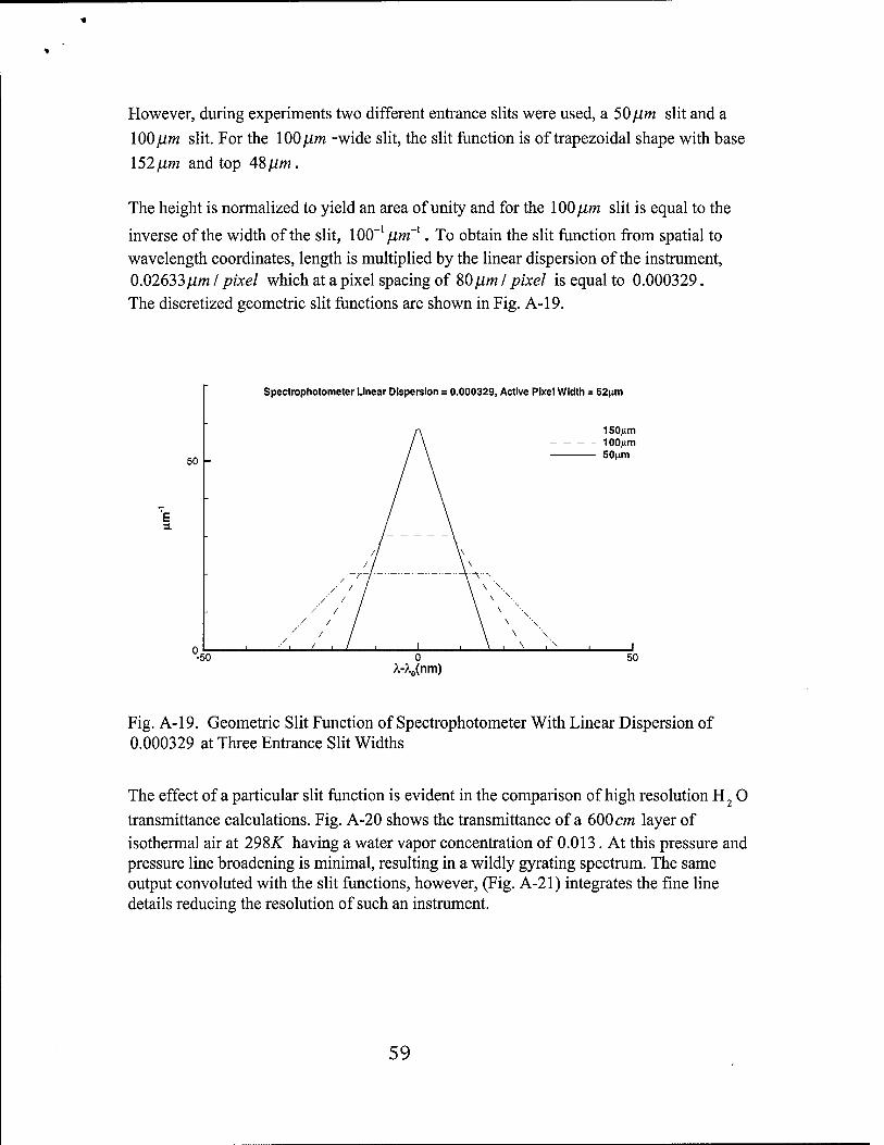
However, during experiments two different entrance slits were used, a 50 jim slit and a 100//m slit. For the 100 jim -wide slit, the slit function is of trapezoidal shape with base \52ßm and top 4Sfim.
The height is normalized to yield an area of unity and for the lOO^um slit is equal to the
inverse of the width of the slit, 100-1//m~'. To obtain the slit function from spatial to wavelength coordinates, length is multiplied by the linear dispersion of the instrument, 0.02633jUm / pixel which at a pixel spacing of SOfim I pixel is equal to 0.000329. The discretized geometric slit functions are shown in Fig. A-19.
Spectrophotometer Linear Dispersion = 0.000329, Active Pixel Width = 52|im
150nm 100|.im 50|xm
E
A-X„(nm)
Fig. A-19. Geometric Slit Function of Spectrophotometer With Linear Dispersion of 0.000329 at Three Entrance Slit Widths
The effect of a particular slit function is evident in the comparison of high resolution H2 O transmittance calculations. Fig. A-20 shows the transmittance of a 600 cm layer of isothermal air at 29%K having a water vapor concentration of 0.013. At this pressure and pressure line broadening is minimal, resulting in a wildly gyrating spectrum. The same output convoluted with the slit functions, however, (Fig. A-21) integrates the fine line details reducing the resolution of such an instrument.
59

T=298 K, Plotal=1atm, PH2O=0.013atm, Resolutions.0001 urn
2.6 2.8 Wavelength X, (\im)
Fig. A-20. TransmittanceofH2OinAir(r=298i:, P=\atm, PH o=0.0l3atm ,
Pathlength=600 cm )
Gaussian Narrow-Band Filter
To consider the effects of recording a finely detailed spectral signal through narrow band filters of varying half-widths, the line-by-line model output is convoluted with a gaussian- shaped filter function. The four-camera imaging system utilizes narrow band filters of 50, 100 and 150 ßm half-widths whose exact transmissive properties are difficult to model. The gaussian function was chosen to approximate the behavior of the filters whose transmissivity was assumed to follow:
Ta-A0)=Ciexp(-C2(A-A0)2) (A42)
where: T= the transmissivity of the filter at wavelength A,
c- *, ln(l/2)
.2 '
A-A0= the deviation from the center wavelength A0 and bh= the half-width of the filter.
Three discretized gaussian profiles used to approximate narrow-band filters are shown in Fig. A-22.
60

1 --
0.8
8 i °-6 E w c 2 H 0.4
0.2
T=298 K, Ptoa,=1 atm, PH2O=0.013atm, Resolution=0.0001 jxm
50nm lOOfxm 150|xm
J i_ _l I L. 2.4 2.6 2.8
Wavelength X, (um)
Fig. A-21. Transmittance of H2 O in Air (T=298K, P=\atm, PH o=0M3atm,
Pathlength= 600 cm ) Convoluted Through Slit Functions of Three Entrance Slit Widths
20
E 10
0 l-J- -100
A.-X0(nm)
150nm 100nm 50nm
100
Fig. A-22. Gaussian Profiles of Varying Half-Width Used for Approximating Convolution by Narrow-Band Filters
61

0.8 -
I i °-6 'E </> c 2 H 0.4
0.2 -
T=298 K, P,ola,=1 atm, PH2O=0.013atm, Resolution=0.0001 |im
50nm 100nm 150nm
J I I l I L. 2.4 2.6 2.8
Wavelength X, (urn)
Fig. A-23. Transmittance of H2 O in Air (T=298K, P=\atm, PHO=0.0\3atm,
Pathlength=600 cm ) Convoluted Through Gauss-Profile Narrow-Band Filters of Three Half- Widths
The wavelength-integrating effects of band filters are shown by the comparison of a detailed spectra such as that of Fig. A-20, and its convolution through the Gaussian profiles of three half-widths in Fig. A-23. All detailed spectra is lost through the integration of narrow high- intensity lines over regions where they are absent.
62


![6. Morante Mat Green Energy v3[1]](https://img.pdfslide.us/doc/110x75/577cd5461a28ab9e789a57f6/6-morante-mat-green-energy-v31.jpg)