Embed Size (px)
Citation preview
V2: Measures and Metrics (II)
- Betweenness Centrality
- Groups of Vertices
- Transitivity
- Reciprocity
- Signed Edges and Structural Balance
- Similarity
- Homophily and Assortative Mixing
SS 2014 - lecture 2 Mathematics of Biological Networks1
Betweenness
Betweenness measures the extent to which a vertex lies
on paths between other vertices.
The idea is usually attributed to Freeman (1977), but was already proposed
in an unpublished technical report by Anthonisse a few years earlier.
Vertices with high betweenness centrality may have considerable influence within
a network e.g. by virtue of their control over information passing between others
(think of data packages in a message-passing scenario).
The vertices with highest betweenness are the ones whose removal from the
network will disrupt most communications between other vertices.
2SS 2014 - lecture 2 Mathematics of Biological Networks
Betweenness Centrality
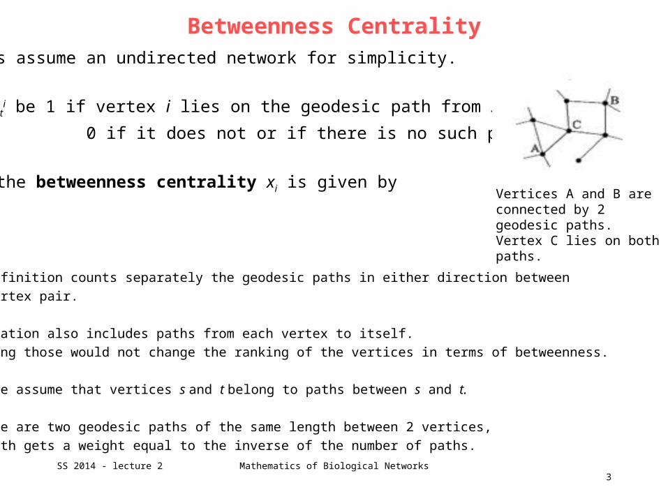
Let us assume an undirected network for simplicity.
Let nsti be 1 if vertex i lies on the geodesic path from s to t
and 0 if it does not or if there is no such path.
Then the betweenness centrality xi is given by
This definition counts separately the geodesic paths in either direction between
each vertex pair.
The equation also includes paths from each vertex to itself.
Excluding those would not change the ranking of the vertices in terms of betweenness.
Also, we assume that vertices s and t belong to paths between s and t.
If there are two geodesic paths of the same length between 2 vertices,
each path gets a weight equal to the inverse of the number of paths.
3SS 2014 - lecture 2 Mathematics of Biological Networks
Vertices A and B areconnected by 2 geodesic paths.Vertex C lies on bothpaths.
Betweenness Centrality
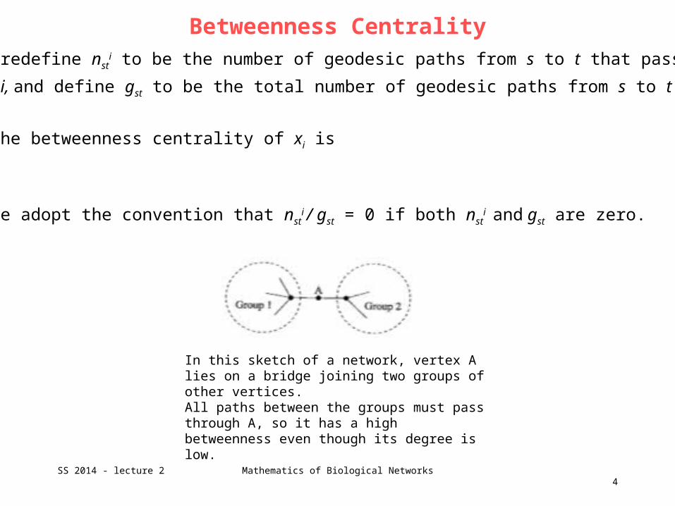
We may redefine nsti to be the number of geodesic paths from s to t that pass through
vertex i, and define gst to be the total number of geodesic paths from s to t.
Then, the betweenness centrality of xi is
where we adopt the convention that nsti / gst = 0 if both nst
i and gst are zero.
4SS 2014 - lecture 2 Mathematics of Biological Networks
In this sketch of a network, vertex A lies on a bridge joining two groups of other vertices. All paths between the groups must pass through A, so it has a high betweenness even though its degree is low.
Range of Betweenness Centrality
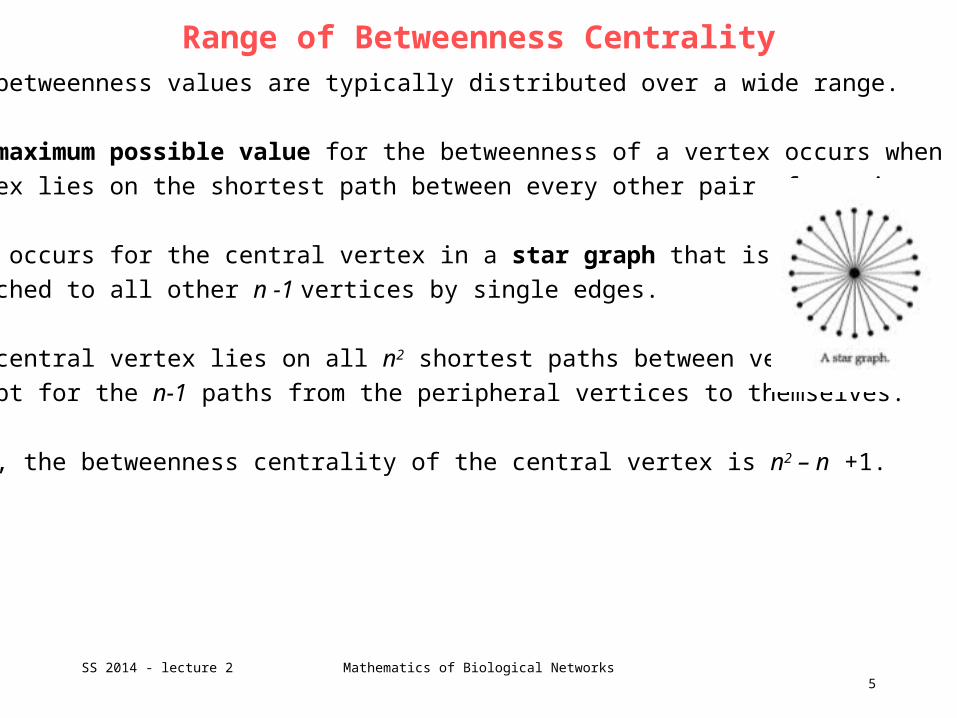
The betweenness values are typically distributed over a wide range.
The maximum possible value for the betweenness of a vertex occurs when the
vertex lies on the shortest path between every other pair of vertices.
This occurs for the central vertex in a star graph that is
attached to all other n -1 vertices by single edges.
The central vertex lies on all n2 shortest paths between vertex pairs
except for the n-1 paths from the peripheral vertices to themselves.
Thus, the betweenness centrality of the central vertex is n2 – n +1.
5SS 2014 - lecture 2 Mathematics of Biological Networks
Range of Betweenness Centrality
In contrast, the smallest possible value of betweenness in a network with a
single component is 2n – 1,
since at a minimum each vertex lies on every path that starts or ends with itself.
There are n – 1 paths from others to the vertex,
n – 1 paths from a vertex to others and
one path from the vertex to itself.
In total, this gives 2 n – 1.
This situation occurs, for instance, when a network has a „leaf“ attached to it,
which is a vertex connected to the rest of the network by just a single edge.
The ratio of largest and smallest possible betweenness values is thus
For large networks, this range of values can become very large.
6SS 2014 - lecture 2 Mathematics of Biological Networks
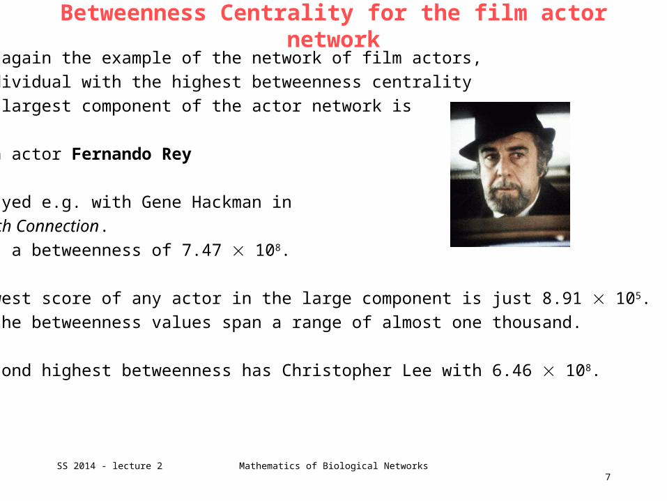
Betweenness Centrality for the film actor networkTaking again the example of the network of film actors,
the individual with the highest betweenness centrality
in the largest component of the actor network is
Spanish actor Fernando Rey
who played e.g. with Gene Hackman in
The French Connection.
Rey has a betweenness of 7.47 108.
The lowest score of any actor in the large component is just 8.91 105.
Thus, the betweenness values span a range of almost one thousand.
The second highest betweenness has Christopher Lee with 6.46 108.
7SS 2014 - lecture 2 Mathematics of Biological Networks
Groups of VerticesMany networks divide naturally into groups or communities.
In lectures V3 and V4, we will discuss some sophisticated computer methods
that have been developed for detecting groups, such as hierarchical clustering
and spectral clustering.
Today, we will start with cliques, plexes, cores, and components.
A clique is a subset of the vertices in an undirected network such that
every member of the set is connected by an edge to every other member.
Newman defines cliques as maximal cliques so that there is no other vertex
in the network that can be added to the subset while preserving the
property that every vertex is connected to every other.
Other scientists distinguish between cliques and maximal cliques.
8SS 2014 - lecture 2 Mathematics of Biological Networks
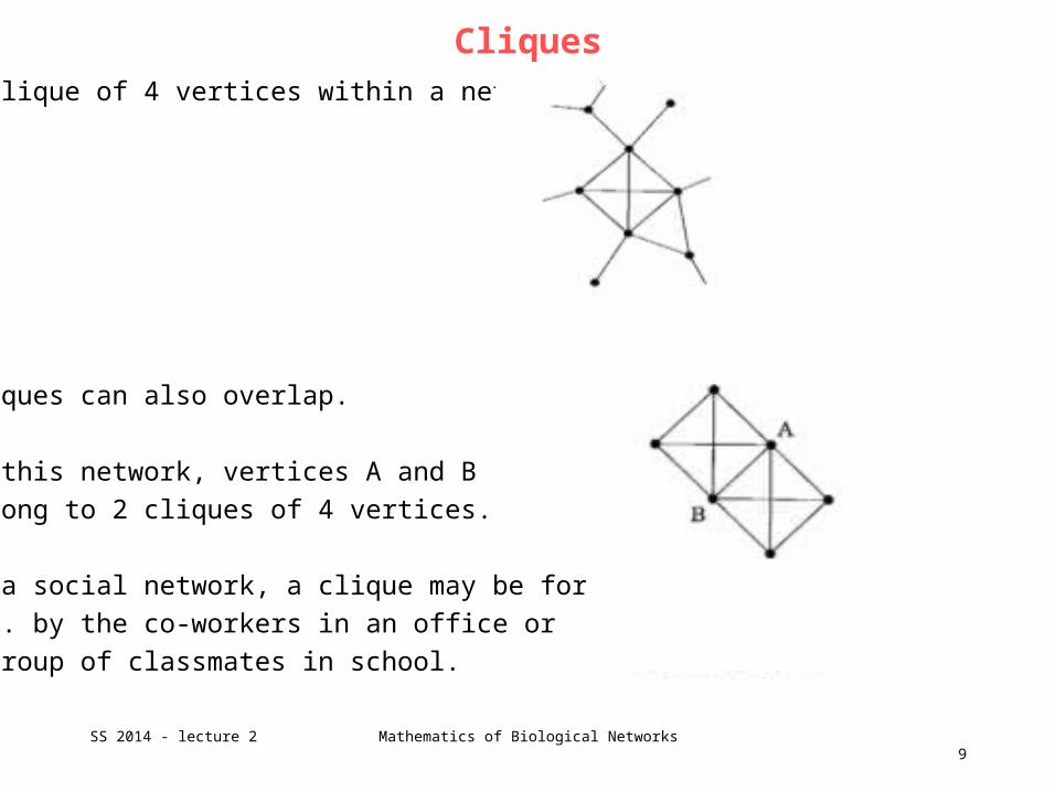
CliquesA clique of 4 vertices within a network.
Cliques can also overlap.
In this network, vertices A and B
belong to 2 cliques of 4 vertices.
In a social network, a clique may be formed
e.g. by the co-workers in an office or
a group of classmates in school.
9SS 2014 - lecture 2 Mathematics of Biological Networks
k-plexOften, many circles of friends form only near-cliques rather than perfect cliques.
One way to relax the stringent requirement that every member is connected to
every other member is the k-plex.
A k-plex of size n is a maximal subset of n vertices within a network such that
each vertex is connected to at least n – k of the others.
A 1-plex is the same as a clique.
In a 2-plex, each vertex must be connected to all or all-but-one of the others.
And so forth.
One can also specify that each member should be connected to a certain
fraction (75% or 50%) of the other vertices.
10SS 2014 - lecture 2 Mathematics of Biological Networks
k-coreThe k-core is another concept that is closely related to the k-plex.
A k-core is a maximal subset of vertices such that each is connected to at
least k others in the subset.
Obviously, a k-core of n vertices is also an (n – k)-plex.
However, the set of all k-cores for a given value of k is not the same as the set of all k-plexes for
any value of k, since n, the size of the group, can vary from one k-core to another.
Also, unlike k-plexes and cliques, k-cores cannot overlap.
The k-core is of particular interest in network analysis for the practical
reason that it is very easy to find the set of all k-cores in a network.
11SS 2014 - lecture 2 Mathematics of Biological Networks
k-core: simple algorithmA simple algorithm is to start with the whole network and remove from it any
vertices that have degree less than k.
Such vertices cannot under any circumstances be members of a k-core.
In doing so, one will normally also reduce the degrees of some other vertices
in the network that were connected to the vertices just removed.
So we go through the network again to see if there are any more vertices
that now have degree less than k and, if there are, we remove those too.
We repeatedly prune the network until no vertices remain with degree < k.
What is left, is by definition a k-core or a set of k–cores.
12SS 2014 - lecture 2 Mathematics of Biological Networks
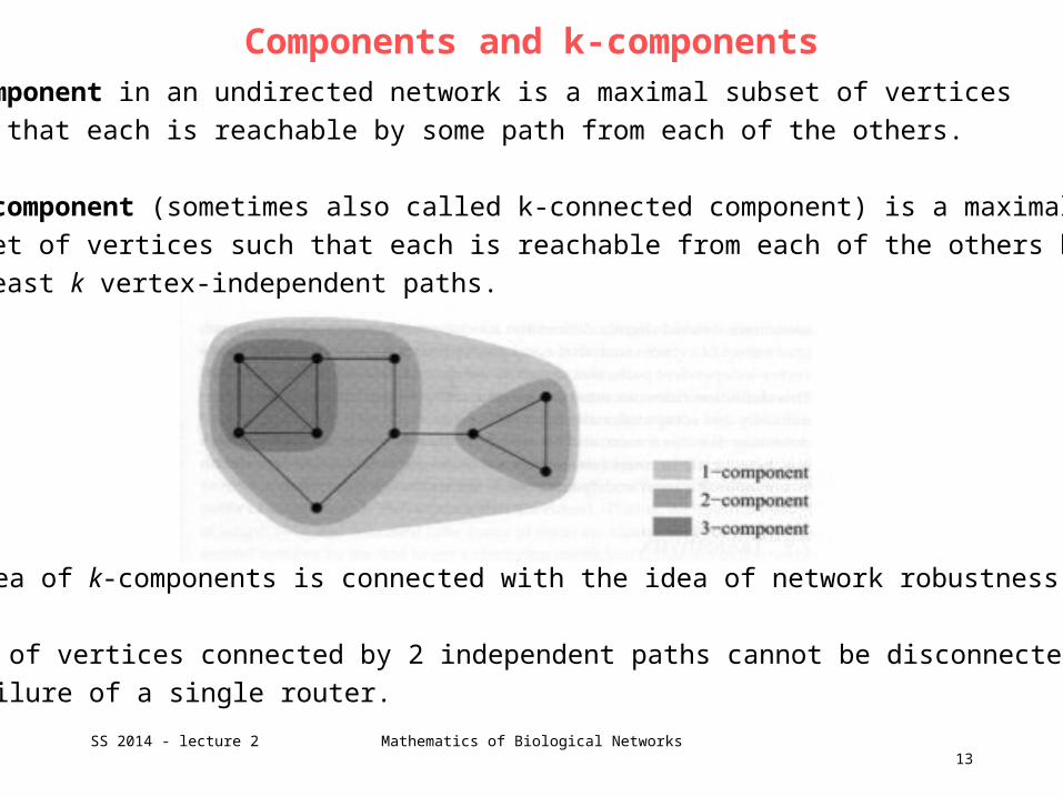
Components and k-componentsA component in an undirected network is a maximal subset of vertices
such that each is reachable by some path from each of the others.
A k-component (sometimes also called k-connected component) is a maximal
subset of vertices such that each is reachable from each of the others by
at least k vertex-independent paths.
13SS 2014 - lecture 2 Mathematics of Biological Networks
The idea of k-components is connected with the idea of network robustness.
A pair of vertices connected by 2 independent paths cannot be disconnected by
the failure of a single router.
TransitivityA property very important in social networks, and useful to a lesser degree in
other networks too, is transitivity.
If the „connected by an edge“ relation were transitive, it would mean that if
vertex u is connected to vertex v, and v is connected to w, then u is also
connected to w.
Perfect transitivity only occurs in networks where each component is a fully
connected subgraph or clique. Perfect transitivity is therefore pretty much a
useless concept for understanding networks.
However, partial transitivity can be very useful.
In many networks, particularly social networks, the fact that u knows v, and
v knows w, doesn‘t guarantee that u knows w but makes it much more likely.
14SS 2014 - lecture 2 Mathematics of Biological Networks
Transitivity
15SS 2014 - lecture 2 Mathematics of Biological Networks
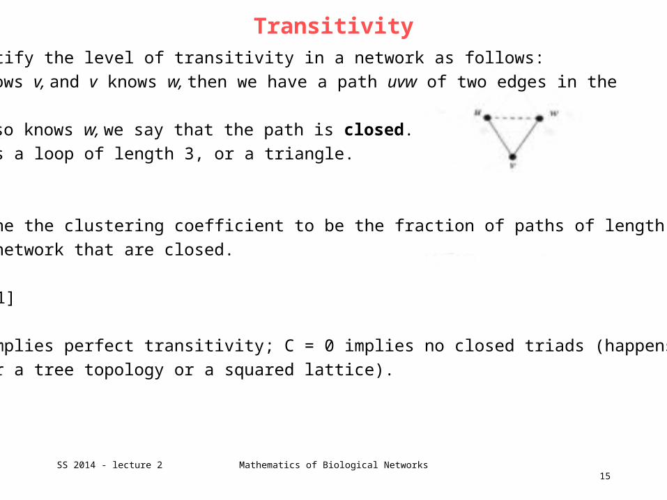
We quantify the level of transitivity in a network as follows:
if u knows v, and v knows w, then we have a path uvw of two edges in the
network.
If u also knows w, we say that the path is closed.
It forms a loop of length 3, or a triangle.
We define the clustering coefficient to be the fraction of paths of length 2
in the network that are closed.
C [0,1]
C = 1 implies perfect transitivity; C = 0 implies no closed triads (happens
e.g. for a tree topology or a squared lattice).
Transitivity
16SS 2014 - lecture 2 Mathematics of Biological Networks
Social networks tend to have quite high values of the clustering coefficient.
E.g. the network of film actor collaborations has C = 0.20
A network of collaborations between biologists has C = 0.09
A network of who sends email to whom in a large university has C = 0.16.
These are typical values of social networks.
Reciprocity
17SS 2014 - lecture 2 Mathematics of Biological Networks
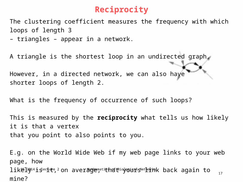
The clustering coefficient measures the frequency with which loops of length 3
– triangles – appear in a network.
A triangle is the shortest loop in an undirected graph.
However, in a directed network, we can also have
shorter loops of length 2.
What is the frequency of occurrence of such loops?
This is measured by the reciprocity what tells us how likely it is that a vertex
that you point to also points to you.
E.g. on the World Wide Web if my web page links to your web page, how
likely is it, on average, that yours link back again to mine?
Reciprocity
18SS 2014 - lecture 2 Mathematics of Biological Networks
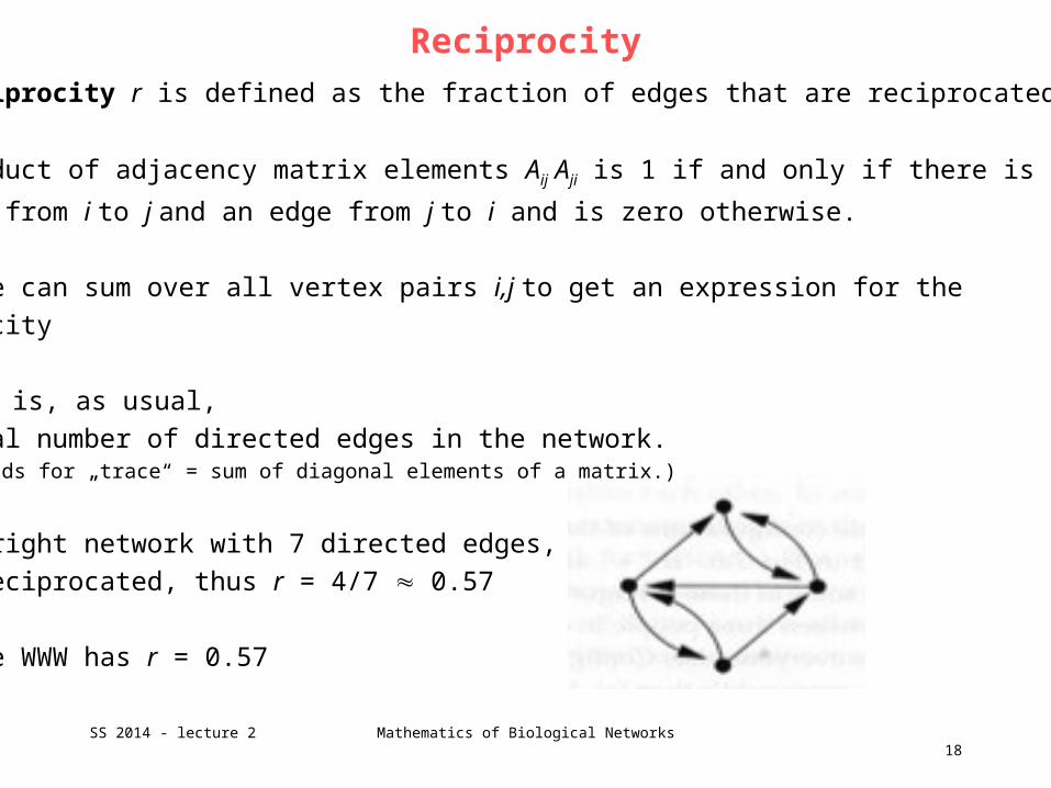
The reciprocity r is defined as the fraction of edges that are reciprocated.
The product of adjacency matrix elements Aij Aji is 1 if and only if there is
an edge from i to j and an edge from j to i and is zero otherwise.
Thus, we can sum over all vertex pairs i,j to get an expression for the
reciprocity
where m is, as usual,
the total number of directed edges in the network. („Tr“ stands for „trace“ = sum of diagonal elements of a matrix.)
In the right network with 7 directed edges,
4 are reciprocated, thus r = 4/7 0.57
Also the WWW has r = 0.57
Signed edges and structural balance
19SS 2014 - lecture 2 Mathematics of Biological Networks
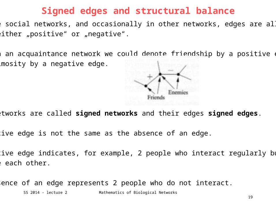
In some social networks, and occasionally in other networks, edges are allowed
to be either „positive“ or „negative“.
E.g. in an acquaintance network we could denote friendship by a positive edge
and animosity by a negative edge.
Such networks are called signed networks and their edges signed edges.
A negative edge is not the same as the absence of an edge.
A negative edge indicates, for example, 2 people who interact regularly but
dislike each other.
The absence of an edge represents 2 people who do not interact.
Signed edges and structural balance
20SS 2014 - lecture 2 Mathematics of Biological Networks
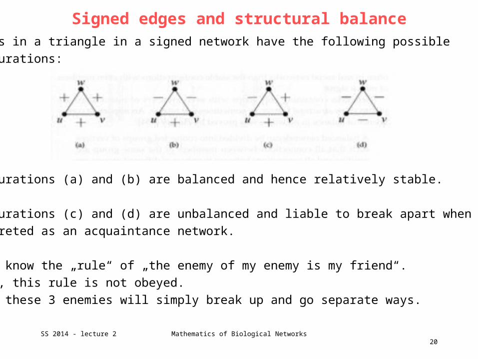
3 edges in a triangle in a signed network have the following possible
configurations:
Configurations (a) and (b) are balanced and hence relatively stable.
Configurations (c) and (d) are unbalanced and liable to break apart when
interpreted as an acquaintance network.
We all know the „rule“ of „the enemy of my enemy is my friend“.
In (d), this rule is not obeyed.
Likely these 3 enemies will simply break up and go separate ways.
Signed edges and structural balance
21SS 2014 - lecture 2 Mathematics of Biological Networks
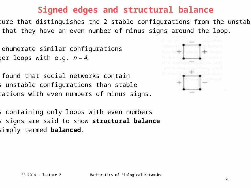
The feature that distinguishes the 2 stable configurations from the unstable
ones is that they have an even number of minus signs around the loop.
One can enumerate similar configurations
for longer loops with e.g. n = 4.
Surveys found that social networks contain
far less unstable configurations than stable
configurations with even numbers of minus signs.
Networks containing only loops with even numbers
of minus signs are said to show structural balance
or are simply termed balanced.
Structural balance
22SS 2014 - lecture 2 Mathematics of Biological Networks
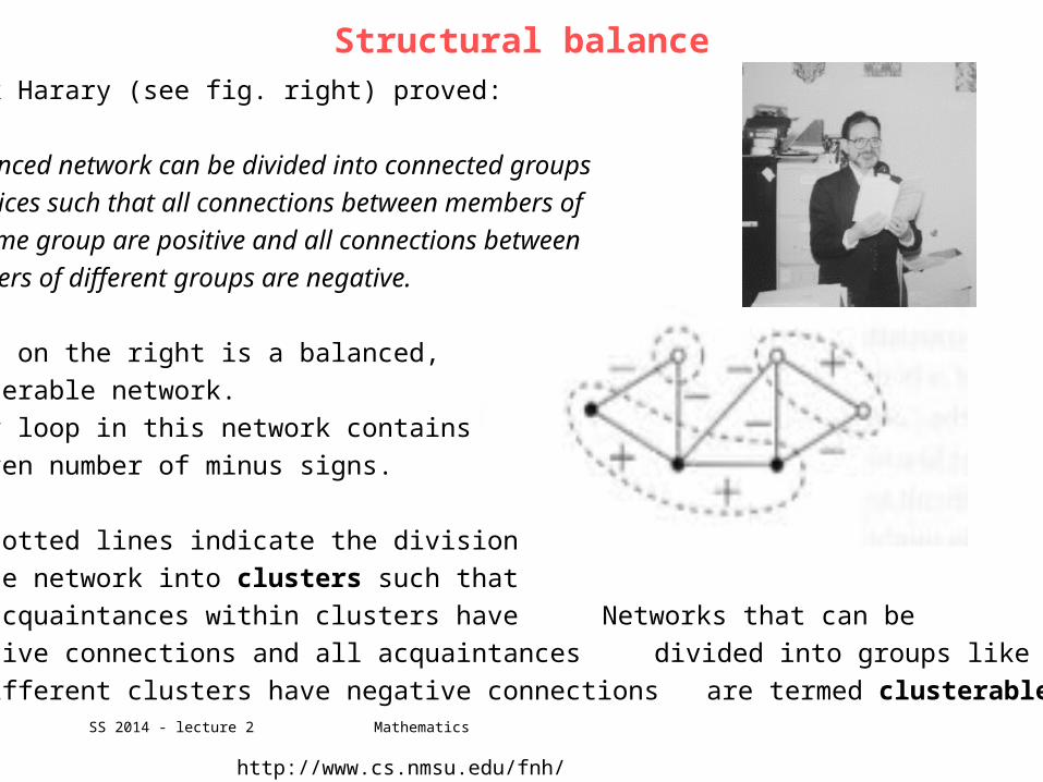
Frank Harary (see fig. right) proved:
A balanced network can be divided into connected groups
of vertices such that all connections between members of
the same group are positive and all connections between
members of different groups are negative.
Shown on the right is a balanced,
clusterable network.
Every loop in this network contains
an even number of minus signs.
The dotted lines indicate the division
of the network into clusters such that
all acquaintances within clusters have Networks that can be
positive connections and all acquaintances divided into groups like this
in different clusters have negative connections are termed clusterable.
http://www.cs.nmsu.edu/fnh/
Proof of Harary’s theorem
23SS 2014 - lecture 2 Mathematics of Biological Networks
Let us start by considering connected networks (they have one component).
We start with an arbitrary vertex and color it in one of two colors.
Then we color the other vertices according to the following algorithm:
1. A vertex v connected by a positive edge to another u that has already been
colored gets the same color as u.
2. A vertex v connected by a negative edge to another u that has already been
colored gets colored in the opposite color from u.
For most networks we may come upon a vertex whose color has already been
assigned.
Then, a conflict may arise between this already assigned color and the new
color that we would like to assign to it.
Proof of Harary’s theorem
24SS 2014 - lecture 2 Mathematics of Biological Networks
We will now show that this conflict can only arise if the network as a whole
is unbalanced.
If while coloring a network we arrive at a already colored vertex, there must
be another path by which this vertex can be reached from our starting point.
→ there is at least one loop in the network to which this vertex belongs.
If the network is balanced, every loop to which our vertex belongs must have
an even number of negative edges around it.
Let us suppose that the color already assigned to the vertex is in conflict
with the one we would like to assign it now.
There are 2 ways in which this could happen.
Proof of Harary’s theorem
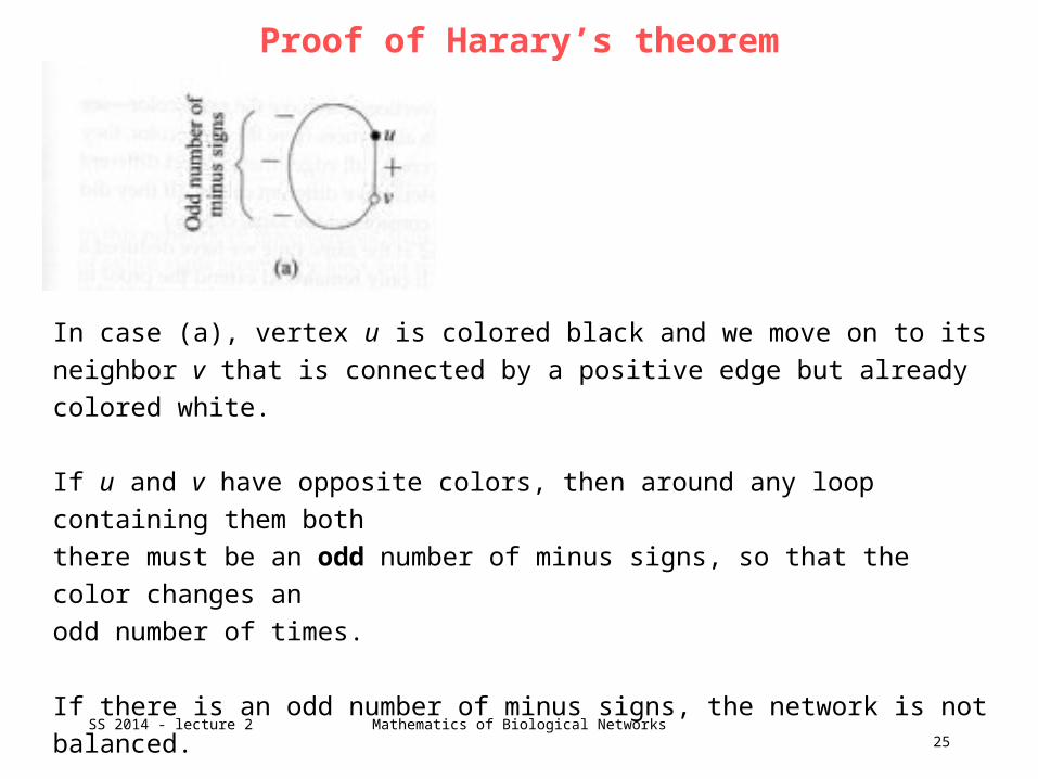
25SS 2014 - lecture 2 Mathematics of Biological Networks
In case (a), vertex u is colored black and we move on to its neighbor v that is
connected by a positive edge but already colored white.
If u and v have opposite colors, then around any loop containing them both
there must be an odd number of minus signs, so that the color changes an
odd number of times.
If there is an odd number of minus signs, the network is not balanced.
Proof of Harary’s theorem
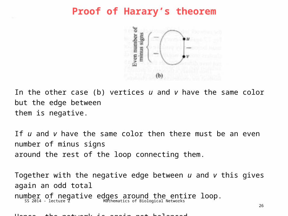
26SS 2014 - lecture 2 Mathematics of Biological Networks
In the other case (b) vertices u and v have the same color but the edge between
them is negative.
If u and v have the same color then there must be an even number of minus signs
around the rest of the loop connecting them.
Together with the negative edge between u and v this gives again an odd total
number of negative edges around the entire loop.
Hence, the network is again not balanced.
Proof of Harary’s theorem
27SS 2014 - lecture 2 Mathematics of Biological Networks
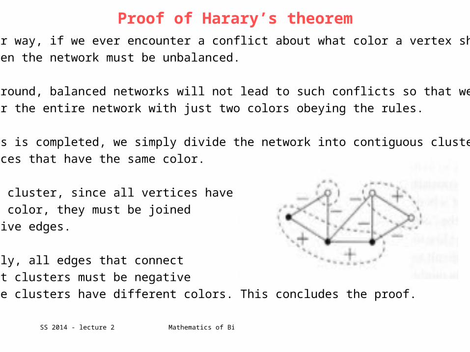
In either way, if we ever encounter a conflict about what color a vertex should
have, then the network must be unbalanced.
Turned around, balanced networks will not lead to such conflicts so that we
can color the entire network with just two colors obeying the rules.
When this is completed, we simply divide the network into contiguous clusters
of vertices that have the same color.
In every cluster, since all vertices have
the same color, they must be joined
by positive edges.
Conversely, all edges that connect
different clusters must be negative
since the clusters have different colors. This concludes the proof.
Proof of Harary’s theorem
28SS 2014 - lecture 2 Mathematics of Biological Networks
Our proof of Harary‘s theorem also led to a method for constructing the clusters.
The proof can be easily extended to networks with more to one component
because we could simply repeat the proof for each component separately.
The practical importance of Harary‘s theorem is based on the observation that
many real social networks are found naturally to be in a balanced or mostly
balanced state.
Is the inverse of this theorem also true?
Are clusterable networks necessarily balanced?
Clusterable networks
29SS 2014 - lecture 2 Mathematics of Biological Networks
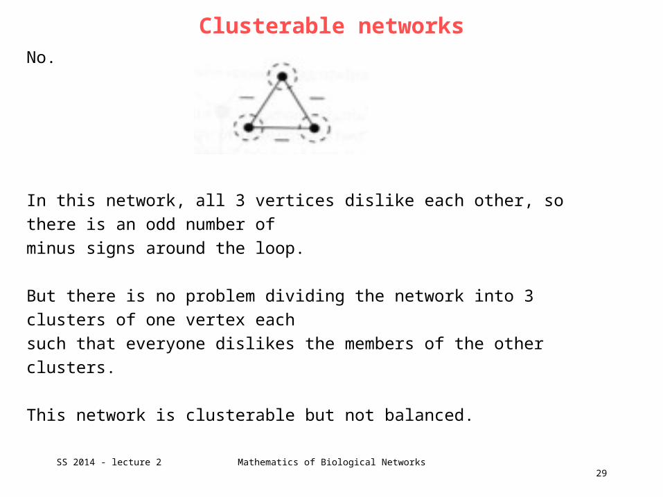
No.
In this network, all 3 vertices dislike each other, so there is an odd number of
minus signs around the loop.
But there is no problem dividing the network into 3 clusters of one vertex each
such that everyone dislikes the members of the other clusters.
This network is clusterable but not balanced.
Similarity
30SS 2014 - lecture 2 Mathematics of Biological Networks
Another central concept in social networks is that of similarity between vertices.
E.g. commercial dating services try to match people with others based on
presumed similarity of their interests, backgrounds, likes and dislikes.
For this, one would likely use attributes of the vertices.
Here, we will restrict ourselves to determining similarity between the vertices
of a network using the information contained in the network structure.
There are two fundamental approaches for constructing meaures of network
similarity, called structural equivalance and regular equivalence.
Structural equivalence
31SS 2014 - lecture 2 Mathematics of Biological Networks
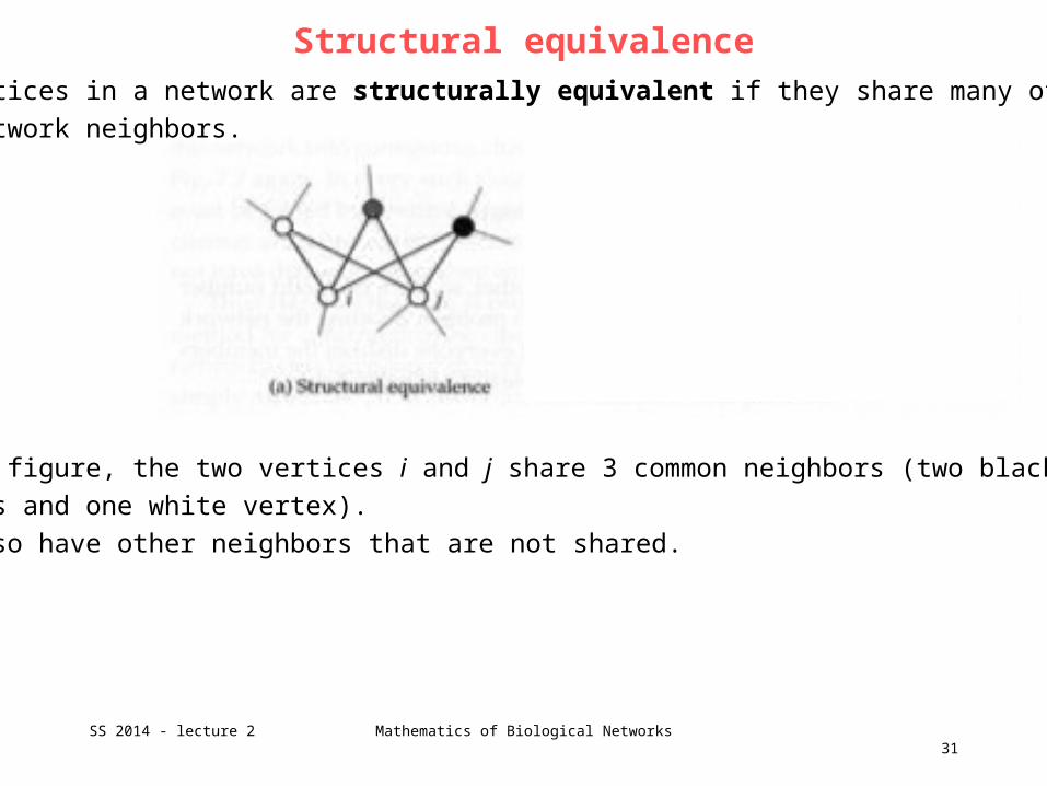
Two vertices in a network are structurally equivalent if they share many of the
same network neighbors.
In this figure, the two vertices i and j share 3 common neighbors (two black
vertices and one white vertex).
Both also have other neighbors that are not shared.
Regular equivalence
32SS 2014 - lecture 2 Mathematics of Biological Networks
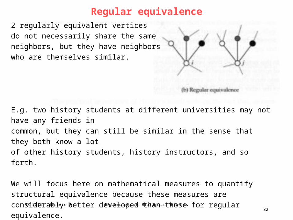
2 regularly equivalent vertices
do not necessarily share the same
neighbors, but they have neighbors
who are themselves similar.
E.g. two history students at different universities may not have any friends in
common, but they can still be similar in the sense that they both know a lot
of other history students, history instructors, and so forth.
We will focus here on mathematical measures to quantify structural equivalence
because these measures are considerably better developed than those for
regular equivalence.
Cosine similarity
33SS 2014 - lecture 2 Mathematics of Biological Networks
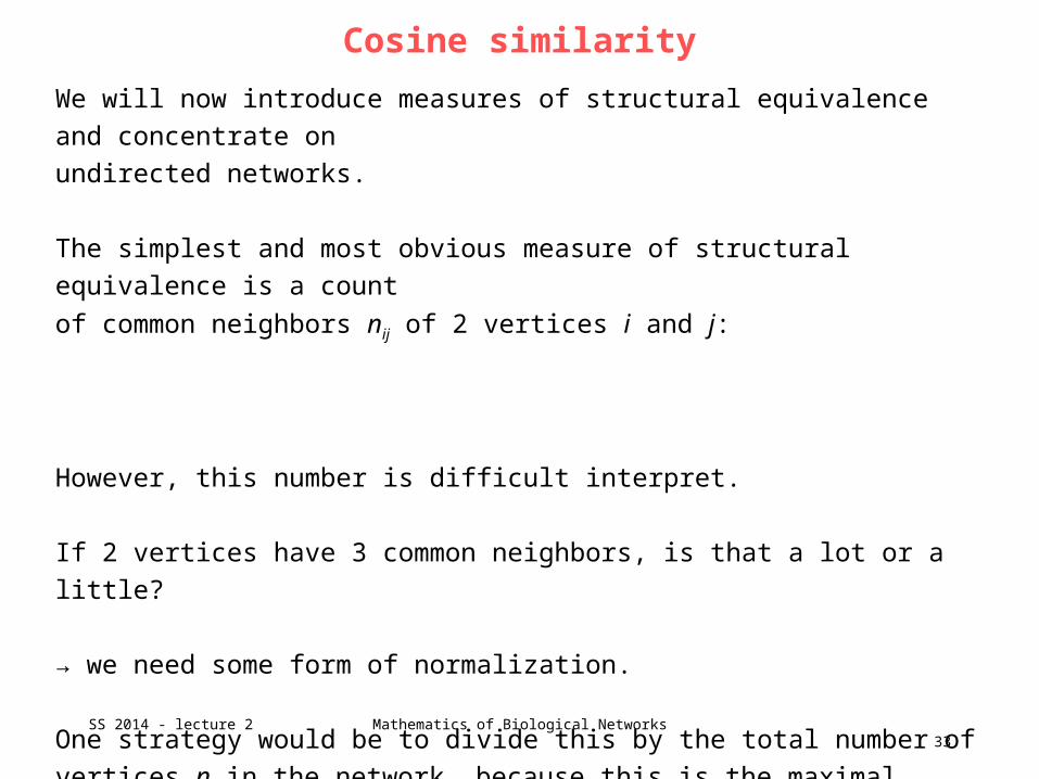
We will now introduce measures of structural equivalence and concentrate on
undirected networks.
The simplest and most obvious measure of structural equivalence is a count
of common neighbors nij of 2 vertices i and j:
However, this number is difficult interpret.
If 2 vertices have 3 common neighbors, is that a lot or a little?
→ we need some form of normalization.
One strategy would be to divide this by the total number of vertices n in the
network, because this is the maximal possible number of common neighbors.
Cosine similarity
34SS 2014 - lecture 2 Mathematics of Biological Networks
However, this would penalize vertices with low degree.
A better measure would allow for the varying degree of vertices.
Such a measure is the cosine similarity.
In geometry, the inner or dot product of 2 vectors x and y is given by
x ∙ y = |x| |y| cos, where |x| is the magnitude of x and the angle between
the 2 vectors.
Rearranging, we can write the cosine of the angle as
Cosine similarity
35SS 2014 - lecture 2 Mathematics of Biological Networks
Salton proposed that we regard the i-th and j-th rows (or columns) of the
adjacency matrix as two vectors and use the cosine of the angle between
them as similarity measure.
By noting that the dot product of two rows is
this gives us the following similarity
Assuming our network is an unweighted simple graph, the elements of the
adjacency matrix take on only the values 0 and 1, so that Aij2 = Aij for all i,j.
Cosine similarity
36SS 2014 - lecture 2 Mathematics of Biological Networks
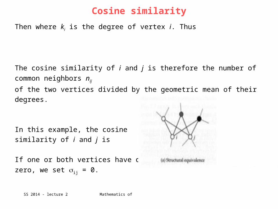
Then where ki is the degree of vertex i. Thus
The cosine similarity of i and j is therefore the number of common neighbors nij
of the two vertices divided by the geometric mean of their degrees.
In this example, the cosine
similarity of i and j is
If one or both vertices have degree
zero, we set ij = 0.
Pearson coefficients
37SS 2014 - lecture 2 Mathematics of Biological Networks
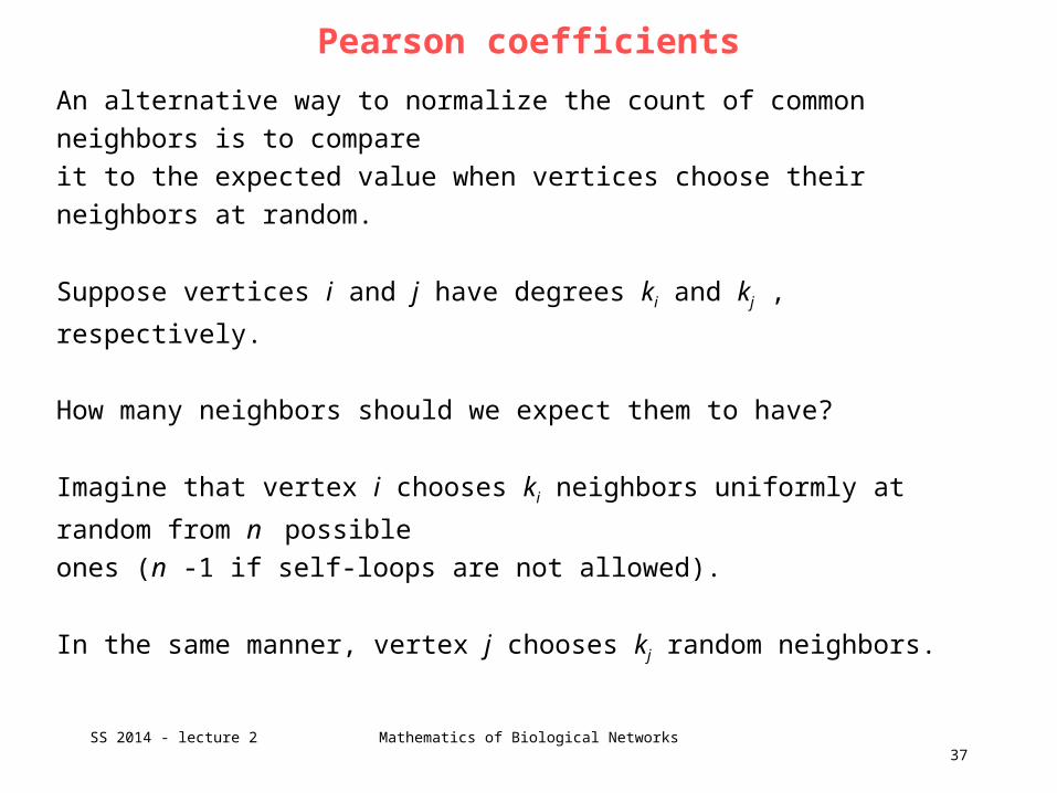
An alternative way to normalize the count of common neighbors is to compare
it to the expected value when vertices choose their neighbors at random.
Suppose vertices i and j have degrees ki and kj , respectively.
How many neighbors should we expect them to have?
Imagine that vertex i chooses ki neighbors uniformly at random from n possible
ones (n -1 if self-loops are not allowed).
In the same manner, vertex j chooses kj random neighbors.
Pearson coefficients
38SS 2014 - lecture 2 Mathematics of Biological Networks
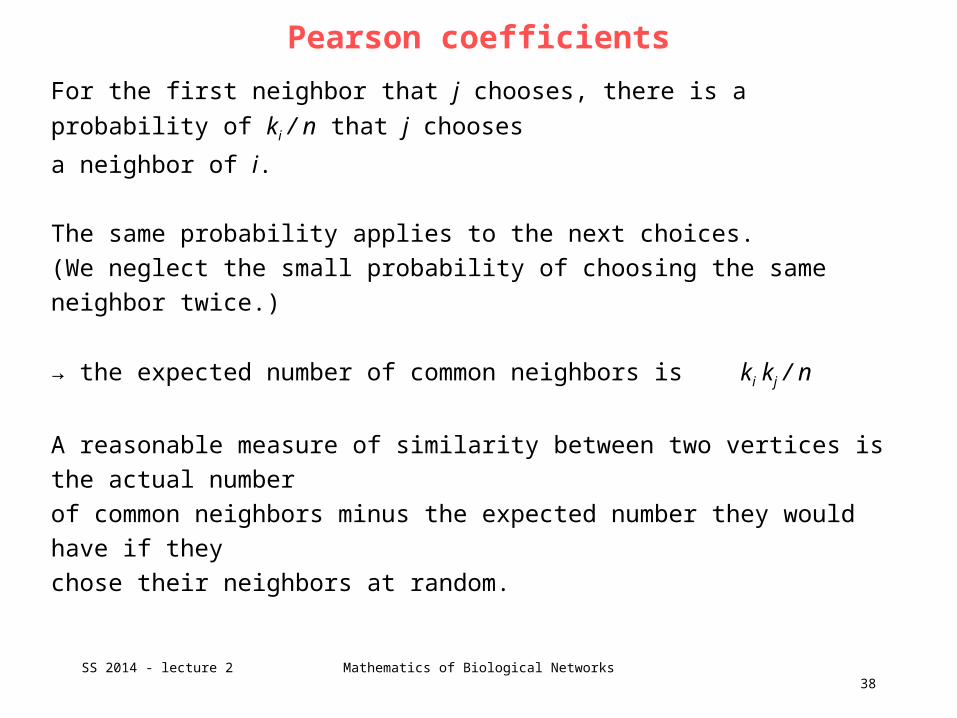
For the first neighbor that j chooses, there is a probability of ki / n that j chooses
a neighbor of i.
The same probability applies to the next choices.
(We neglect the small probability of choosing the same neighbor twice.)
→ the expected number of common neighbors is ki kj / n
A reasonable measure of similarity between two vertices is the actual number
of common neighbors minus the expected number they would have if they
chose their neighbors at random.
Pearson coefficients
39SS 2014 - lecture 2 Mathematics of Biological Networks
Here <Ai> denotes the mean of the elements of the i th row of
the adjacency matrix.
This equation is n times the covariance cov(Ai,Aj) of the two rows of the
adjacency matrix.
Pearson coefficients
40SS 2014 - lecture 2 Mathematics of Biological Networks
Normalizing this as we did with the cosine similarity, so that it ranges between
-1 and 1, gives the standard Pearson correlation coefficient
Homophily or Assortative Mixing
41SS 2014 - lecture 2 Mathematics of Biological Networks
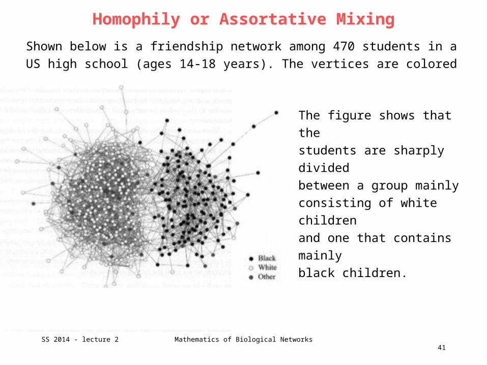
Shown below is a friendship network among 470 students in a US high school
(ages 14-18 years). The vertices are colored by race.
The figure shows that the
students are sharply divided
between a group mainly
consisting of white children
and one that contains mainly
black children.
Homophily or Assortative Mixing
42SS 2014 - lecture 2 Mathematics of Biological Networks
This observation is very common in social networks.
People have apparently a strong tendency to associate with others whom
they perceive as being similar to themselves in some way.
This tendency is termed homophily or assortative mixing.
Assortative mixing is also seen in some nonsocial networks,
e.g. in citation networks where papers from one field cite papers from the
same field.
How can one quantify assortative mixing?
Quantify assortative mixing
43SS 2014 - lecture 2 Mathematics of Biological Networks
Find the fraction of edges that run between vertices of the same type
and subtract from this the fraction of edges we would expect if edges
were positioned at random without regard for vertex type.
ci : class or type of vertex i , ci [1 … nc]
nc : total number of classes
The total number of edges between vertices of the same type is
Here (m,n) is the Kronecker delta ( is 1 if m = n and 0 otherwise).
The factor ½ accounts for the fact that every vertex pair i,j is counted
twice in the sum.
Quantify assortative mixing
44SS 2014 - lecture 2 Mathematics of Biological Networks
Now we turn to the expected number of edges between vertices if the edges
are placed randomly.
Consider a particular edge attached to vertex i which has degree ki.
By definition, there are 2m ends of edges in the entire network where m is the
total number of edges.
If connections are made randomly, the chances that the other end of our
particular edge is one of the kj ends attached to vertex j is thus kj / 2m.
Counting all ki edges attached to i , the total expected number of edges
between vertices i and j is then ki kj / 2m
Quantify assortative mixing
45SS 2014 - lecture 2 Mathematics of Biological Networks
The expected number of edges between all pairs of vertices of the same type is
where the factor ½ avoids double-counting vertex pairs.
Taking the difference between the actual and expected number of edges gives
=
Typically one does not calculate the number of such edges but the fraction,
which is obtained by dividing this by m
This quantity Q is called the modularity. In the student network Q=0.305.
Assortative mixing by scalar characteristics
46SS 2014 - lecture 2 Mathematics of Biological Networks
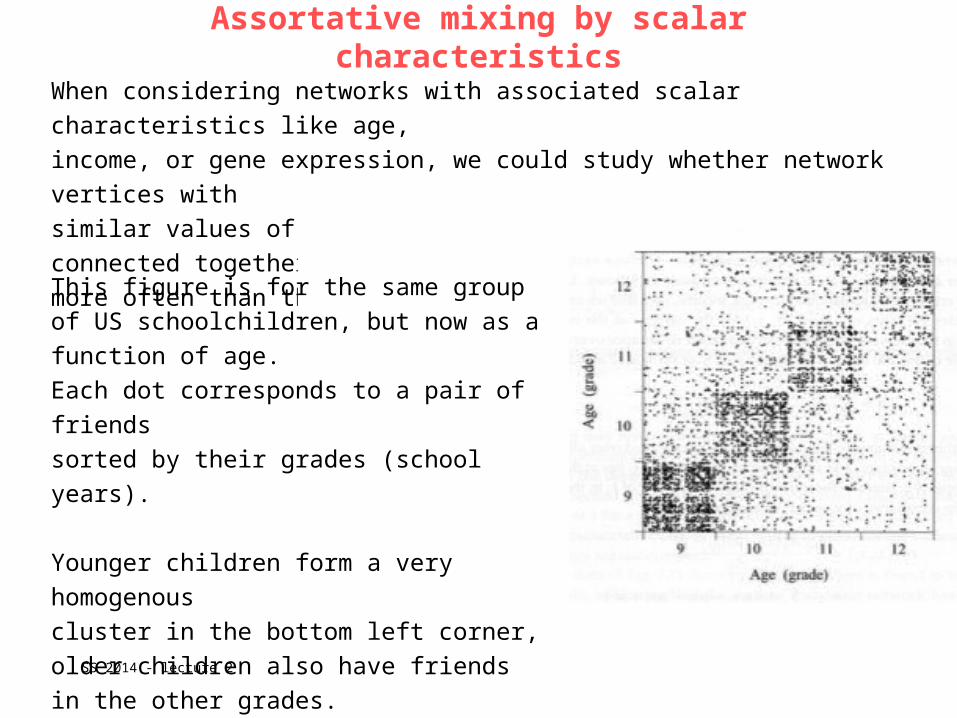
When considering networks with associated scalar characteristics like age,
income, or gene expression, we could study whether network vertices with
similar values of this scalar characteristics tend to be connected together
more often than those with different values.
This figure is for the same group of US
schoolchildren, but now as a function of age.
Each dot corresponds to a pair of friends
sorted by their grades (school years).
Younger children form a very homogenous
cluster in the bottom left corner, older children
also have friends in the other grades.
Assortative mixing by scalar characteristics
47SS 2014 - lecture 2 Mathematics of Biological Networks
A good way of quantifying this tendency is by the covariance (no derivation
here):
where now replaces the Kronecker symbol.


![Fully Dynamic Betweenness Centrality Maintenance on ... · work analysis software such as SNAP [26], WebGraph [9], Gephi, NodeXL, and NetworkX. Betweenness centrality measures the](https://img.pdfslide.us/doc/110x75/5f8999eb65d3911b1622e646/fully-dynamic-betweenness-centrality-maintenance-on-work-analysis-software-such.jpg)
![Randomized flow model and centrality measure for electrical ......the betweenness centrality measure of [16] is computed, to more realistically capture the importance of the role played](https://img.pdfslide.us/doc/110x75/60f7b3fe8fba690d5c20f68c/randomized-flow-model-and-centrality-measure-for-electrical-the-betweenness.jpg)


![spcl.inf.ethz.chspcl.inf.ethz.ch/Publications/.pdf/pushpull-slides.pdf · spcl.inf.ethz.ch @spcl_eth 1. Forward traversals BETWEENNESS CENTRALITY BRANDES [1] [1] U. Brandes. A faster](https://img.pdfslide.us/doc/110x75/5f93dd3f74a1c70c3d675e39/spclinfethz-spclinfethzch-spcleth-1-forward-traversals-betweenness-centrality.jpg)