arX

iv:0

911.

2759

v1 [

nlin

.PS]

14

Nov

200

9

Wave patterns within the generalizedconvection–reaction–diffusion equation1

V. Vladimirov2

Faculty of Applied MathematicsUniversity of Science and Technology

Mickiewicz Avenue 30, 30-059 Krakow, Poland

Abstract. A set of travelling wave solutions to a hyperbolic generalization of the convection-

reaction-diffusion is studied by the methods of local nonlinear alnalysis and numerical simulation.

Special attention is paid to displaying appearance of the compactly supported soloutions, shock fronts,

soliton-like solutions and peakons

PACS codes: 02.30.Jr; 47.50.Cd; 83.10.Gr

Keywords: generalized convection-reaction-diffusion equation, compactons, peakons,shock fronts, soliton-like travelling wave solutions

1 Introduction

As is well-known, there do not exist methods of obtaining the general solutions to mostof non-linear evolutionary PDEs. Very often in such circumstances the only alterna-tive to numerical studies of nonlinear models deliver the symmetry-based methods [1].An important sub-class of the self-similar solutions is formed by the travelling wave(TW) solutions. The object of this study is to demonstrate the existence of a numberof localized self-similar TW solutions, basing on the hyperbolic generalization of theconvection-reaction-diffusion equation. We pay special attention to the existence ofsolitary waves [2], shock fronts [3] and some other generalized solutions, such as com-pactons and peakons [4, 5, 6]. The structure of the study is following. In section 2we introduce our model equation and next factorize it to an ODE, describing the setof TW solutions. Next we discuss the geometric interpretation of solitary waves andoutline the way of capturing them. In sections 3 and 4 we perform the local nonlinearanalysis of the dynamical system, equivalent to the factorized ODE, purposed at stat-ing conditions of the wave patterns occurrence. In section 5, we present the results ofnumerical study, revealing the presence of all above mentioned types of TW solutions.Finally, in section 6, we discuss the results obtained and outline the ways of furtherinvestigations.

1The research was supported by the AGH local grant2E-mail address: vsevolod.vladimirov@gmai.com

1

2 Statement of the problem

We consider the following evolutionary equation (referred to as GBE):

αutt + ut + u ux − κ (un ux)x = (u− U1)ϕ(u). (1)

Here n, κ, U1 are positive constants, α is nonnegative. Equation (1) is a generalizationof both Burgers equation and the reaction-diffusion equation. Let us note, that theterm αutt appears when the memory effects are taken into account [8, 9, 10, 11]. Someparticular cases of equation (1) were studied in recent years [12, 13, 14, 15, 11, 16].Owing to these studies, the analytical description of a large variety of travelling wave(TW) solutions is actually available.

Present investigations are mainly devoted to the qualitative and numerical study ofthe family of TW solution to GBE. Our aim is to show that under certain conditionsthe set of TW solutions contains solitons, compactons, peakons and some other wavepatterns. To put it briefly, we maintain the notation traditionally used in more specificsense. Thus, soliton is usually associated with the exponentially localized invariant TWsolution to a completely integrable equations, possessing a number of unusual features[2]. Some of these features are also inherited by the compactons [17, 18]. We maintainthe notion to those solutions to (1), which manifest similar geometric features as ”true”wave patterns, known under these names.

Let us consider the set of TW solutions

u(t, x) = U(ξ) ≡ U (x− V t) . (2)

Inserting ansatz (2) into the GBE, one can obtain, after some manipulation, the fol-lowing dynamical system:

∆(U) U = ∆(U)W,

∆(U) W = (U − V ) W − κ nUn−1W 2 − ϕ(U) (U − U1)

where ∆(U) = κ Un − αV 2. By analyzing the factorized system (3), we are going toformulate the conditions contributing to the appearance of the soliton-like solutions andthe solutions with compact support, called compactons, and some types of generalizedTW solutions. Analysis carried out, e.g. in [5, 7] shows, that homoclinic trajectoriesbi-asymptotic to saddle points correspond to both soliton-like and compacton-like so-lutions. In the first case the homoclinic loop is bi-asymptotic to a simple saddle, hence,the ”time” which is necessary to penetrate such trajectory is infinite. The closed looprepresenting the compacton is bi-asymptotic to a topological saddle. As a result, the”time” of penetration is finite. In fact, the compacton is is a compound generalizedsolution. Its compactly supported nonzero part corresponds to the closed loop, whilethe rest corresponds to the stationary point.

In order to ”capture” the homoclinic trajectory among the other solutions to thesystem (3), we are going to state the condition, which guarantee the stable limit cycleappearance. Choice of such strategy is based upon the well-known fact that the growth

2

of the radius of the limit cycle in presence of a nearby saddle point most often leads tothe homoclinic bifurcation. Application of this prescription to the system (3) occursto have some peculiarities, which are characterized below.

1. The most natural parameter of the bifurcation is the wave pack velocity V . Yetits change causes the movement of the line of singular points ∆(U) = 0 (singularline for brevity) in the horizontal direction. As will be shown below, the presenceof the topological saddle in most cases is due to the fact that the saddle pointbelongs to the singular line. On account of this, the problem of ”capturing” thecompacton-like solution becomes more complicated, for one must ”synchronize”the moment of the homoclinic bifurcation with the passage of the singular linethrough the saddle point.

2. Presence of the singular line delivers an extra mechanism of the limit cycle de-struction, competing with the mechanism based upon the homoclinic loop for-mation.

3. When the far end of the limit cycle approaches the singular line just at themoment of the homoclinic loop formation, the latter becomes flat and remindstriangle. Such loop corresponds to a different type of the generalized solutions,called peakons [5, 6].

4. The singular line is unmovable when α = 0. In this case, corresponding to theparabolic-type model, the analysis becomes much more easy, [19].

3 Andronov–Hopf bifurcation in the system (3)

The homoclinic bifurcation can occur in the system (3) if it has an extra stationarypoint. The function

ϕ(U) = (U − U0)m ψ(U), 0 ≤ U0 < U1,

considered throughout the remaining part of the work, assures the required geometricconfiguration, providing that ψ(U) does not change sign within the segment [U0, U1].

To formulate the conditions which guarantee the limit cycle appearance in vicinityof the stationary point (U1, 0), let us consider the Jacobi matrix

J1 =

(

0 ∆(U1)−ϕ(U1) U1 − V

)

.

In order that (U1, 0) be a center, the eigenvalues of J1 should be pure imaginary. Thisis so if the conditions

Trace J1 = U1 − V = 0, (3)

DetJ1 = ∆(U1) (U1 − U0)m ψ(U1) > 0 (4)

3

are fulfilled. The first condition immediately gives us the critical value of the wave packvelocity Vcr1 = U1. The second one is equivalent to the statement that both ∆(U1) andψ(U1) are nonzero and have the same signs.

The next thing we are going to do is a study of the stability of the limit cycle. As iswell known [20, 21], this is the real part of the first Floquet index ℜC1 that determinesthe stability of the periodic trajectory. Depending on the sign of ∆(U1), there are twopossibilities. If ∆(U1) > 0 when V = Vcr1 or, in other words, the horizontal coordinateof the singular line ∆(U∗) = 0, corresponding to the critical value of the parameter V ,satisfies the inequality

U∗ (Vcr1) =

[

αVcr12

κ

]

1

n

< U1,

then conditions ψ(U1) > 0, and ℜC1 < 0 should be fulfilled. In case when U∗ (Vcr1) >U1, these parameters should have the opposite signs.

To obtain the expression for ℜC1, the standard formula contained e.g. in [21] canbe directly applied, provided that our system is presented in the following form:

(

z1z2

)

=

(

0 −ΩΩ 0

)

·(

z1z2

)

+

(

F (z1, z2)G(z1, z2)

)

, (5)

where Ω =√µ · ν, µ = |∆(U1)|, ν = |ϕ(U1)|, F (z1, z2) and G(z1, z2) stand for nonlinear

terms. In this (canonical) representation ℜC1 is expressed as follows [21]:

16ℜC1 = F111 + F122 +G112 +G222 +1

ΩF12 (F11 + F22)−

−G12 (G11 +G22) − F11G11 + F22G22 . (6)

By Fijk, Fij we denote the coefficients of the function’s F (z1, z2) monomials zi zj zk,zi zj correspondingly. Similarly, indices Gij Gijk denote the coefficient of the secondand third order monomials of the function G(z1, z2).

A passage to the canonical variables (z1, z2) can be attained by the unified trans-formation. If the relations (3)–(4) are satisfied, then, rewriting (3) in the coordinatesy1 = U − U1, y2 = W , we get the following system:

∆(U)d

d ξ

(

y1

y2

)

=

(

0 ǫ µ−ǫ ν 0

) (

y1

y2

)

+

(

Φ1(y1, y2)Φ2(y1, y2)

)

, (7)

where

ǫ =

+1 if ∆(U1) > 0,−1 if ∆(U1) < 0,

Φ1(y1, y2) = κ nUn−21 y1 y2

(

U1 +n− 1

2y1

)

+O(

|yi|4)

, (8)

Φ2(y1, y2) = −1

2y2

1 (2ϕ(U1) + ϕ(U1) y1) − κnUn−21 y2

2 (U1 + (n− 1)y1) + y1 y2 +O(

|yi|4)

.

4

In order to pass to the standard representation, we apply the change of coordinates:(

z1z2

)

=

(

−ǫ√ν 00

õ

)

·(

y1

y2

)

.

This gives us the system (5), with

F (z1, z2) =κ nUn−2

1

Ωz1 z2

[√ν U1 − ǫ

n− 1

2z1

]

+O(|zi|4), (9)

G(z1, z2) =µ

2 νΩz21

[

ǫ ϕ(U1)z1 − 2 ϕ(U1)√ν]

− ǫ

õ

Ωz1 z2 −

−κ nUn−21

Ωz22

[

U1

√ν − ǫ (n− 1) z1

]

+O(|zi|4).

The real part of the Floquet index is easily calculated from (9):

ℜC1 = − 1

16 ΩG12 (G11 +G22) = −ǫ 1

16 Ω2 |ϕ(U1)|

|∆(U1)| ϕ(U1) + κ n|ϕ(U1)|Un−11

.

(10)The above can be summarized in the form of the following statement.

Theorem 1. If ∆(U1) · ψ(U1) > 0, and

|∆(U1)| ϕ(U1) + κ n|ϕ(U1)|Un−11 > 0, (11)

then in vicinity of the critical value of the wave pack velocity Vcr1 = U1 a stable limitcycle appears.

4 Study of the stationary point (U0, 0)

Rewriting (3) in the coordinates X = U − U0, W we obtain the system

∆(U0 +X) X = ∆(U0 +X)W,

∆(U0 +X) W = [(U1 − U0) −X] Xm ψ (U0 +X)−−κ n (U0 +X)n−1 W 2 + (U0 − V +X) W,

(12)

where ∆(U0 + X) = κ [(U0 +X)n − αD2]. Our aim is to determine the conditionsensuring that the stationary point X = W = 0 is a topological saddle, or, at least,contains a saddle sector in the right half-plane. The standard theory [22] can be appliedfor this purpose. Our system can be written down in the form

d

d T

(

XW

)

=

(

0 ∆(U0)A U0 − V

) (

XW

)

+ nonl. terms, (13)

where dd T

= ∆(U0 +X) dd ξ

,

A =

(U1 − U0 ) ψ(U0), if m = 1,0, if m ≥ 2.

5

The linearization matrix of the system (13) is nonsingular if m = 1 and the point U∗

lies outside the segment [U0, U1]. In this case the stationary point (0, 0) is a simplesaddle and the homoclinic trajectory corresponds to the solitary wave solution. Outof this case, the Jacobi matrix has at leas one zero eigenvalue. To study the behaviorof dynamical system in vicinity of a degenerated stationary point, we use the resultsfrom [22]. Since we are interested in the case when the trace of the Jacobi matrix isnonzero, the analysis prescribed in Chapter IX of [22] is the following.

1. Find the change of variables (U, X, T ) 7→ (x, y, τ) enabling to write down thesystem (13) in the standard form

d x

d τ= P2 (x, y) ,

d y

d τ= y +Q2 (x, y) ,

where P2 (x, y), Q2 (x, y) are polynomials of degree 2 or higher.

2. Solve the equation y + Q2 (x, y) = 0 with respect to y, presenting the result inthe form of the decomposition y = a1 x

µ1 + a2 xµ2 + ....

3. Find the asymptotic decomposition

P2 (x, y(x)) = ∆m xm + ....

4. Depending on the values of m and the sign of ∆m, select the type of the complexstationary point, using the theorem 65 from [22].

5. Return to the original variables (U, X, T ) and analyze whether the geometry ofthe problem allows for the homoclinic bifurcation appearance.

So let us present the results obtained for the system (12). First we assume, that m >1, the statements of the Andronov-Hopf theorem are fulfilled and the point U∗ satisfyingthe equation ∆(U∗) = 0 lies outside the segment [U0, U1], when the parameter V reachesthe second bifurcation value Vcr2, corresponding to the homoclinic bifurcation. Herewe have three possibilities.

• U∗ > U1 when the Andronov-Hopf bifurcation occurs (i.e. V = Vcr1). Thisinequality does not change up to the homoclinic bifurcation, when V = Vcr2 >Vcr1.

• The inequalities U0 < U∗ < U1 take place when V = Vcr1 and the inequalitychanges for U∗ < U0 when V belongs to a small neighborhood of Vcr2 < Vcr1.

• U∗ < U0 when the Andronov-Hopf bifurcation occurs (i.e. V = Vcr1). Thisinequality does not change up to the homoclinic bifurcation, when V = Vcr2 <Vcr1.

6

Remark 1. Let us note that in the first case the functions ∆(U) and ψ(U) arenegative when U ∈ [U0, U1]. In the third case both of the functions are positive withinthe given interval. In the second case ψ(U0) is positive, and the factor ∆(U0) changesthe sign from negative to positive as U∗ becomes less than U0.

For m > 1, the canonical system is obtained by the formal change (X, W ) 7→ (x, y),and passage to the new independent variable τ = (U0 − V ) T , in each of the abovecases. As a result of such transformation, we get the following system:

d xd τ

= ∆(U0+x)U0−V

y,= P2(x, y),

d yd τ

= y − 1V−U0

xy − κ n (U0 + x)n−1 y2 + xm [(U1 − U0) − x] [ψ(U0) + ψ′(U0) x+ ....] =

= y +Q2(x, y).(14)

Presenting y in the form of series y = a1 xµ1 + a2 x

µ2 + ... and solving the equationy +Q2(x, y) = 0, we obtain

y = am xm + .... =

U1 − U0

V − U0ψ(U0) x

m + ... (15)

Inserting the function y(x) into the RHS of the first equation, we get

P2(x, y(x)) = − ∆(U0)

(U0 − V )2(U1 − U0)ψ(U0) x

m + .... = ∆m xm + .... (16)

Fulfillment of the statements of the Andronov-Hopf theorem implies that ∆(U1)ψ(U1) >0 when V = Vcr1. Previously we assumed that function ψ(U) does not change signwithin the segment [U0, U1]. And this is suffice to conclude that the product remainspositive, when the parameter V attains the value Vcr2, corresponding to the homo-clinic bifurcation. It is quite evident for the cases one and three, because the line∆(U) = 0 remains on the same side of the segment [U0, U1]. In the case 2 the situa-tion is somewhat different, because ∆(U0) is negative for V = Vcr1, while the functionψ(U0) is positive and remains so when the parameter V changes. But the singular line∆(U) = 0 is located to the left from the point (U0, 0) when V becomes close to Vcr2,and then, in accordance with the Remark 1, the product ∆(U0)ψ(U0) is positive, whenthe homoclinic bifurcation occurs. So the coefficient ∆m in the decomposition (16) isalways negative. Basing on the classification given in Ch. IX of [22], it is possible toformulate the following statement.

Proposition 1. Let the statements of the Theorem 1 be fulfilled and the singularline ∆(U) = 0 lies outside the segment [U0, U1] of the horizontal axis. Then, form ≥ 2 the origin of the system (14) is a topological saddle, having a pair of outgoingseparatrices tangent to the vertical axis and the pair of incoming ones tangent to thehorizontal axis, when m = 2 k, k = 1, 2, .... For m = 2 k + 1, k = 1, 2, 3..., thestationary point is a saddle-node with two saddle sectors lying in the right half-plane.Two outgoing separatrices of the saddle sector are tangent to the vertical axis while theincoming one is tangent to the horizontal axis.

7

In the following, we present the analysis of system’s (12) behavior in vicinity ofthe stationary point (0, 0), assuming that ∆(U0) = 0 when V = Vcr2. The results ofthe study occur to depend on whether or not U0 is equal to zero. But both of thesecases can be analyzed simultaneously. We begin with the case m > 1, for which thecanonical system is obtained by the formal change (X, W ) 7→ (x, y) and passage tothe new independent variable τ = (U0−V )T . As a result, we get the following system:

d xd τ

= κ

U0−V

∑nk=1

n!k!(n−k)!

Un−k0 xk y,= P2(x, y),

d yd τ

= y − 1V−U0

xy − κ n (x+ U0)n−1 y2 + xm [x− (U1 + U0)] [ψ(U0) + ψ′(U0) x+ ...]

=

= y +Q2(x, y).(17)

Presenting y in the form of series y = a1 xµ1 + a2 x

µ2 + ... and solving the equationy + Q2(x, y) = 0, we convince that the first term of the asymptotic decompositiony(x) coincides with (15). This is not surprising, since the second equations of thesystems (14) and (17) are identical. Inserting the function (15) into the RHS of thefirst equation of system (17), we get

P2(x, y(x)) =

−nκ Un−10 ψ(U0)

U1−U0

(U0−V )2xm+1 + ...., if U0 > 0,

−κ ψ(0)U1

V 2 xn+m + ...., if U0 = 0.

In the case m = 1 a passage to the canonical system is attained by means of thetransformation

x = X, y = W +BX, τ = (U0 − V )T,

where

B = ψ(U0)U1 − U0

U0 − V. (18)

In the new variables, our system reads as follows:

d xd τ

= κ

U0−V(y −B x)

∑nk=1

n!k!(n−k)

Un−k0 xk ,= P2(x, y),

d yd τ

= y + 1V−U0

[

κB2 Un−10 (n + 1) +B + ψ(u0)

]

x2 + .... = y +Q2(x, y).

(19)

Solving equation y +Q2(x, y) = 0, we obtain

y =1

U0 − V

[

κB2 Un−10 (n + 1) +B + ψ(u0)

]

x2 + ....

Inserting function y(x) into the RHS of the first equation, we finally get

P2(x, y(x)) =

−κ Un−10 ψ(U0)

U1−U0

(U0−V )2x2 + ... if U0 > 0,

−κ ψ(0) U1

V 2xn+1 + ... if U0 = 0.

8

U

X

m=1

U

X

m³2

Figure 1: Phase portraits of the system (12) in vicinity of the origin for different valuesof the parameter m, in cases when U∗ (Vcr2) = U0

U

X

U*@Vcr2D<U0

U

X

U*@Vcr2D=U0

Figure 2: Phase portraits of the system (12) in vicinity of the origin for m = 1/2

9

So the coefficients of the lowest monomials of the decomposition of P2 (x, y(x)) arenegative and the following statement, based on the classification given in [22], holdstrue for U0 = 0.

Proposition 2.

1. If m ≥ 2, and m + n is an odd natural number, then the origin of the system(17) is a topological saddle having a pair of outgoing separatrices tangent to thevertical axis and the pair of incoming separatrices tangent to the horizontal axis.For even m + n, the stationary point is a saddle-node with two saddle sectorslying in the right half-plane. Its outgoing separatrices are tangent to the verticalaxis while the incoming one is tangent to the horizontal axis. The nodal sectorlying in the left half-plane is unstable.

2. If m = 1, and n is an odd number then the origin of the system corresponding to(19) is a topological saddle identical with that of the previous case. For even n,the stationary point is a saddle-node identical with that of the previous case.

Below we formulate the analogous result for U0 > 0.

Proposition 3.If m = 2 k, k = 1, 2, ..., then, the origin of the system (17) is atopological saddle having a pair of outgoing separatrices, tangent to the vertical axis andthe pair of incoming ones, tangent to the horizontal axis. For m = 2 k+1, k = 1, 2, ...,the stationary point is a saddle-node with two saddle sectors lying in the right half-plane. Its outgoing separatrices are tangent to the vertical axis while the incoming oneis tangent to the horizontal axis. The nodal sector lying in the left half-plane is stable.For m = 1, and arbitrary n ∈ N , the origin of the system corresponding to (19) is asaddle-node identical with that of the case m > 1.

The last case we are going to analyze is that with m = 12. The motivation for such

a choice will be clear later on. In order to be able to apply the analytical theory, werewrite the system (12), introducing new variable Z =

√X:

d ZdT

= κ

2

[

∆(U0) + nUn−10 Z + ...+ Z2n−1

]

W,

dWdT

= W [(U0 − V ) + Z2] − κ n [U0 + Z2]n−1

W 2 + Z [(U1 − U0) − Z2] ψ(U0 + Z2).(20)

Let us consider the Jacobi matrix of the system (20), corresponding to the stationarypoint (0, 0):

J =

[

0 κ

2∆(U0)

ψ(U0)(U1 − U0) (U0 − Vcr2)

]

. (21)

Analysis of the matrix (21) shows, that the origin is a simple saddle when U∗ (Vcr2) liesoutside the segment [U0, U1]. In the case when U∗ (Vcr2) = U0, one of the eigenvaluesof the Jacobi matrix is zero, and, in order to classify the stationary point, we use theresults from [22]. A passage to the canonical variables is attained by means of the

10

transformation

x = Z, y = W +BZ, τ = (U0 − V )T, B =U1 − U0

U0 − Vψ(U0).

The system resulting from this is as follows:

d xd τ

= κ

2 (U0−V )

[

nUn−10 x+ ...+ x2n−1

]

(y − B x) = P2(x, y),

d yd τ

= y − 1(V−U0)

B κ

2

[

nUn−10 x+ ... + x2n−1

]

(y −B x) − x2 (y −B x)−

−κ n [U0 + x2]n−1 − x3 ψ(U0) + ...

= y +Q2(x, y).

(22)

Solving the equation y + Q2(x, y) with respect to y we obtain a series y = a2 x2 +

.... An outlook of this series’ coefficients proves to be unimportant, because they donot contribute to the lowest term of the asymptotic decomposition of the functionP2(x, y(x)), which is as follows:

P2(x, y(x)) =

−κnUn−1

0(U1−U0)ψ(U0)

2 (U0−V )2x2 + ...., if U0 > 0

−κψ(0)2V 2 x2n + ...., if U0 = 0.

Let us formulate the result obtained as the following statement.

Proposition 4.If m = 1/2, then, in case, when U∗ (Vcr2) lies outside the segment[U0, U1], the origin of the system (22) is a simple saddle. In case when U∗ (Vcr2) = 0,the origin of the system (22) is a saddle-node, having two saddle sectors lying in theright half-plane. Its outgoing separatrices are tangent to the vertical axis while theincoming separatrice is tangent to the horizontal axis.

The crucial fact appearing from this analysis is that the stationary points (0, 0) ofthe canonical systems (17), (19) and (22), depending on the values of the parametersm, n, are either saddles or saddle-nodes with the saddle sectors placed at the righthalf-space. The return to the original coordinates does not cause any change in theposition of the saddle sectors, but it changes the orientation of vector fields 3 and theangles, at which the outgoing separatrices leave the stationary point. The local phaseportraits corresponding to the distinct cases are shown in Fig. 1, reconstructed on thebasis of the analysis of the relation between (17)–(19) and the system (12).

Returning to coordinates (X, W ) in the case when m = 1/2, we obtain the patternsof the phase trajectories shown in Fig. 2. The difference between the case whenU∗ (Vcr2) = U0 and when U∗ (Vcr2) lies outside the segment [U0, U1] is not essential -in both cases the incoming and outgoing separatrices enter the origin tangent to thevertical axis. Yet, since in the second case the upper sepratrice is a mirror image

3We assume that U0 − Vcr2< 0, otherwise the presumable homoclinic loop will not correspond to

the wave of ”compression”. Fulfillment of this condition is verified during the numerical simulation

11

of the lower one, then one can expect the compactly supported solution to be moresymmetric.

Before we start to discuss the results of numerical study of the system (12), let usanalyze to what type of solitary waves will correspond the homoclinic loops, presum-ably appearing in system (3). In order to analyze this issue, we are looking for theasymptotic solution W (X) = α1 X

µ1 + α2Xµ2 + ... of the equation

∆(U0 +X)W dWdX

= G ≡

≡ [(U0 − V ) +X) W − κ n (U0 +X)n−1W 2 − ψ(U0 +X) [(U0 − U1) +X] Xm,(23)

which is equivalent to the system (12). Let us start with the case U0 = 0, for whichthe equation (23) can be re-written as follows:

κXn+2µ1−1(

α1 + α2Xµ2−µ1 + ...

) (

µ1 α1 + µ2 α2Xµ2−µ1 + ...

)

=

= X1+µ1

(

α1 + α2Xµ2−µ1 + ...

)

− V Xµ1

(

α1 + α2Xµ2−µ1 + ...

)

− (24)

−κ nXn+2µ1−1(

α21 + 2α1α2X

µ2−µ2 + ....)

−[

Xm+1 + U1

]

Xm ψ(0) + ....

The procedure of solving (24) is pure algebraic: we collect the coefficients of differentpowers of X and equalize them to zero. The lowest power in the RHS is either Xµ1 orXn+2µ1−1. The number n + 2µ1 − 1 cannot be less or equal to µ1, because it involvesthe inequality 0 < µ1 ≤ 1 − n, which is impossible for any natural n. On the otherhand, if n + 2µ1 − 1 ≤ m, then µ1 becomes an ”orphan” and α1 should be nullified.

So Xn+2µ1−1 cannot be the lowest monomial. From this, it immediately appearsthat the only choice leading to a nontrivial solution is µ1 = m.

For U0 > 0 the equation is as follows:

κX2µ1

(

α1 + α2Xµ2−µ1 + ...

) (

µ1 α1 + µ2 α2Xµ2−µ1 + ...

)

=

= ψ(U0)Xm [(U1 − U0) −X] −

−κ n[

Un−10 + ...

] (

α21 X

2µ1 + ...)

+ [X + (U0 − V )] [α1Xµ1 + ...] . (25)

Using the analogous arguments as before for the present (more simple) case, we con-clude that µ1 = m.

The decomposition obtained can be used to asymptotically integrate the equation

dX

d ξ= W = a1X

m + ....

which immediately gives in the lowest order the expression

X =

[a1(1 −m) (ξ − ξ0)]1

1−m , if m 6= 1,

C exp [a1 (ξ − ξ0)], if m = 1,

from which we conclude that the trajectory reaches the origin in ”finite time” if m < 1.

12

Unfortunately, in case when m ∈ N+, presented above result cannot be attributedto both of the saddle sector separatrices, forming the closed loop. In fact, the incomingseparatrix of the stationary point (0, 0) in all cases considered here is tangent to thevertical axis and therefore cannot be described by the formula (26) when m ≥ 1. Theabove formula, then, describes the asymptotic behavior of the ”tail ” of the solitarywave, corresponding to the homoclinic solution.

To complete the analysis, we resort to some arguments, concerning the other end ofthe homoclinic trajectory. It is the common feature of almost all the cases consideredhere, that the incoming separatrice is tangent to the vertical axis, with the exceptionof the case when m = 1 and U∗ (Vcr2) lies outside the interval (U0, U1). This enablesus to assume that in vicinity of the origin W = −B Uσ + o (Uσ), where 0 < σ < 1 andB > 0. An approximate equation describing the first coordinate of the separatrix is,then, as follows

dU

d ξ= −B Uσ + o (Uσ) .

Performing the asymptotic integration, we obtain, up to the change of notation, thesolution identical with (26), concluding from this that in all analyzed above cases withm, n ∈ N+, the incoming separatix reaches the origin in finite ”time”.

It is obvious, that similar arguments can be applied to the analysis of presumablehomoclinic trajectory, corresponding to m = 1/2. It appears from the above analysis,that the incoming and outgoing separatrces are tangent to the vertical axis and bothof them reach the origin in finite ”time”. Let us note that when U∗ (Vcr2) lies outside[U0, U2], the asymptotic behavior of the spearatrices is described by the formula

X = ±√

γ (ξ − ξ0), γ > 0.

So this is the only case when the homoclinic trajectory corresponds with certain to thecompactly supported solution of the equation (1).

5 Results of numerical simulation

Since the parabolic case was discussed in detail in our previous work [19], we mainlyconcentrate here on the hyperbolic case, corresponding to α > 0. Numerical simulationsof the system (12) were carried out with κ = 1, U1 = 3, U2 = 1. The remainingparameters varied from one case to another. The results of qualitative study evidencethat, within the variety of parameters that were analyzed, the only case when whenthe homoclinic loop corresponds to the compactly supported solution is that withm = 1/2. We discuss the results concerning the details of the phase portraits in termsof the reference frame (X, W ). The numerical experiments show that in case whenm = 1/2, n = 1 and U∗ (Vcr2) < U0, both of the separatrices forming closed loop enterthe stationary point (0, 0) tangent to the vertical axis, Fig. 3, the left picture. Theright picture shows the compactly supported solution to Eq. (1), corresponding to theclosed loop. When U∗ (Vcr2) tightly approaches U0, no matter from the left of from theright, the left side of the homoclinic trajectory is clasped to the vertical axis, Fig. 4,

13

1.5 2.0 2.5 3.0 3.5 4.0 4.5X

-2.0

-1.5

-1.0

-0.5

0.0

0.5

1.0W

0 2 4 6 8 10Ξ

1.5

2.0

2.5

3.0

3.5

4.0U

Figure 3: Homoclinic solution of the system (12) with ϕ(U0 + X) = X1/2 (left) andthe corresponding compactly supported TW solution to Eq. (1) (right), obtained forn = 1, α = 0.12, Vcr2

∼= 2.68687 and U∗ − U0 = −0.133684

1.5 2.0 2.5 3.0 3.5 4.0X

-2.0

-1.5

-1.0

-0.5

0.0

0.5

1.0W

0 2 4 6 8Ξ1.0

1.5

2.0

2.5

3.0

3.5

4.0

4.5U

Figure 4: Homoclinic solution of the system (12) with ϕ(U0 + X) = X1/2 (left) andthe corresponding TW solution to Eq. (1) (right), obtained for n = 1, α = 0.13827,Vcr2

∼= 2.68892 and U∗ − U0 = 0.99973

left. The corresponding compactly supported solution has more sharp front, Fig. 4,right.

As it was shown in the previous section, appearance of the soliton-like solutionsis possible merely in case when m = 1. In accordance with the predictions of ourqualitative analysis, such solutions were observed for m = n = 1 and values of theparemeters guaranteeing the fulfillment of the inequality U∗ (Vcr2) < U0. As it is seenon the left picture of Fig. 5, both of the separatrices of the saddle sector form nonzeroangle with the vertical axis and this gives us the reason to state that the homoclinicloop corresponds in this case to the smooth solitary wave, which is nonzero for anyξ ∈ R.

When U∗ tightly approaches U0, the incoming separatrice of the homoclinic tra-jectory is clasped to the vertical axis (Fig. 6, left) and the solutions reminding shockwaves with relaxed tails are observed in place of soliton-like wave packs (Fig. 6, center,right).

For m ≥ 2 merely the shock-like solutions have been observed in numerical experi-ments. This confirms the arguments put forward in the previous section. The outlookof the TW occurs to depend on the values of the parameters m, n. A series of shock-like

14

1.5 2.0 2.5 3.0 3.5 4.0U

-1.5

-1.0

-0.5

0.0

0.5

1.0W

0 20 40 60 80Ξ

1.5

2.0

2.5

3.0

3.5

4.0U

0 5 10 15Ξ

1.5

2.0

2.5

3.0

3.5

4.0U

Figure 5: Homoclinic solution of the system (12) with ϕ(U0 + X) = X1 (left), thecorresponding tandem of well-localized soliton-like solutions to Eq. (1) (center), andthe soliton-like solution (right), obtained for n = 1, α = 0.06, Vcr2

∼= 2.65795 andU∗ − U0 = −0.576119

1.5 2.0 2.5 3.0 3.5 4.0X

-1.5

-1.0

-0.5

0.0

0.5

1.0W

0 10 20 30 40 50

1.5

2.0

2.5

3.0

3.5

4.0

24 26 28 30 32 34 36

1.5

2.0

2.5

3.0

3.5

4.0

Figure 6: Homoclinic solution of the system (12) with ϕ(U0 + X) = X1 (left), thecorresponding tandem od solitary wave solutions to Eq. (1) (center) and a singlesolitary wave solution (right), obtained for n = 1, α = 0.142, Vcr2

∼= 2.65489 andU∗ − U0 = 0.000878617

15

0 10 20 30 40 50Ξ1.0

1.5

2.0

2.5

3.0

3.5

4.0U

0 10 20 30 40 50 60 70Ξ1.0

1.5

2.0

2.5

3.0

3.5

4.0U

0 20 40 60 80 100Ξ1.0

1.5

2.0

2.5

3.0

3.5

4.0U

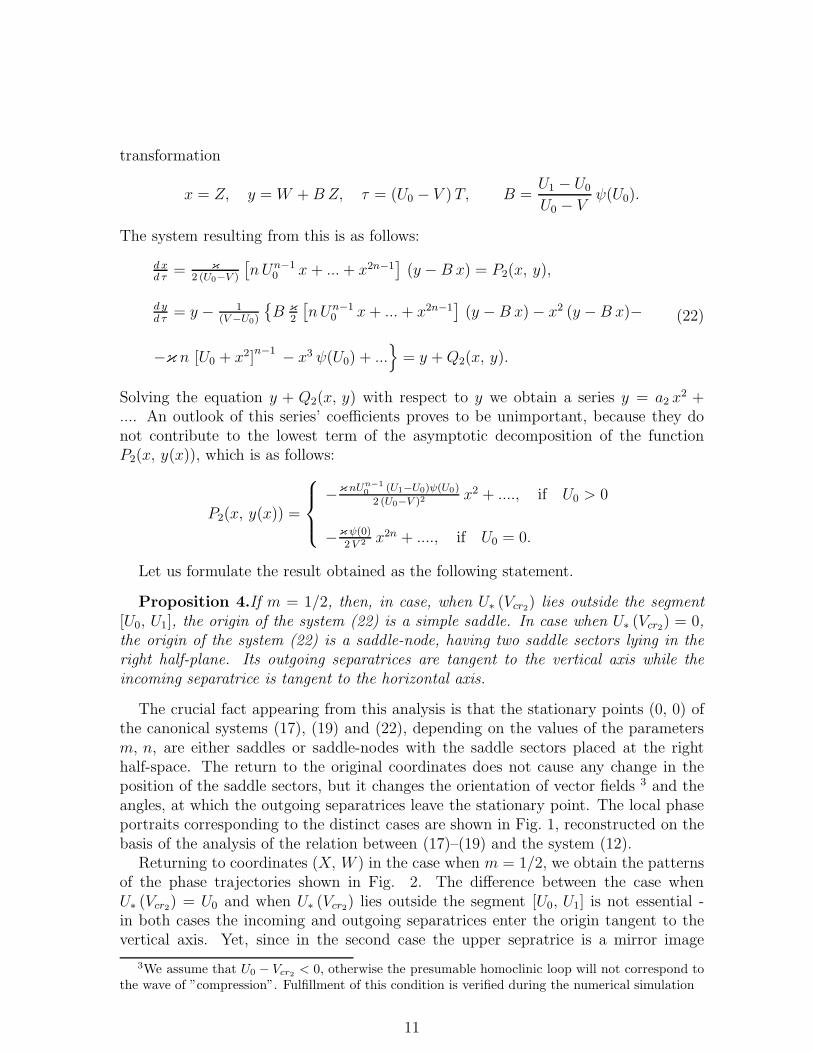
Figure 7: Tandems od shock-like solutions to Eq. (1), corresponding to ϕ(U0 +X) =X1, U∗ ≈ U0, n = 2 (left), n = 3 (center), and n = 4 (right)

0 50 100 150 200Ξ

1.5

2.0

2.5

3.0

3.5

4.0U

0 50 100 150 200Ξ

1.5

2.0

2.5

3.0

3.5

4.0U

0 50 100 150 200Ξ

1.5

2.0

2.5

3.0

3.5

4.0U

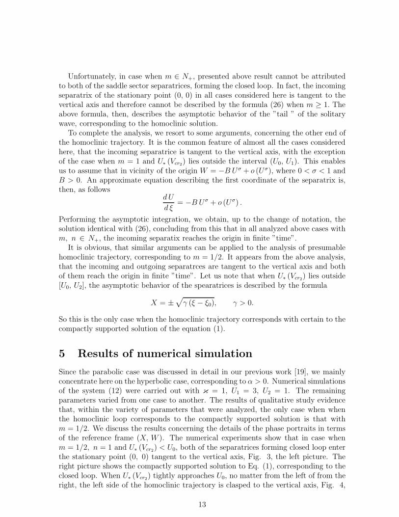
Figure 8: Shock-like solutions to Eq. (1), corresponding to ϕ(U0 +X) = X3, U∗ ≈ U0,n = 1 (left), n = 3 (center), and n = 4 (right)

solutions corresponding to m = 1 and n = 2, 3, 4 are shown in Fig. 7. It is seen, thateffective width of the TW grows as n grows, and the shape becomes more and moregently sloping.

The next series (Fig. 8) shows the TW corresponding to m = 3 and n = 1, 2, 3.This picture differs from the previous one in that the ”tails” of the travelling wavesare longer. A common feature of all the cases with m ≥ 2 is the strong stability of theequilibrium, especially in the direction of the outgoing separatrice. Choosing the initialdata more and more close to the origin, we are able to elongate the ”tail” without limit.Besides, the profiles of the TW become more and more smooth as the n grows.

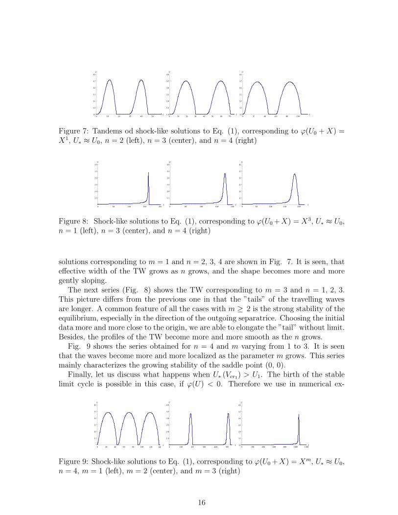
Fig. 9 shows the series obtained for n = 4 and m varying from 1 to 3. It is seenthat the waves become more and more localized as the parameter m grows. This seriesmainly characterizes the growing stability of the saddle point (0, 0).

Finally, let us discuss what happens when U∗ (Vcr1) > U1. The birth of the stablelimit cycle is possible in this case, if ϕ(U) < 0. Therefore we use in numerical ex-

0 20 40 60 80 100 120 140Ξ

1.5

2.0

2.5

3.0

3.5

4.0U

0 100 200 300 400 500Ξ

1.5

2.0

2.5

3.0

3.5

4.0U

0 200 400 600 800 1000 1200Ξ1.0

1.5

2.0

2.5

3.0

3.5

4.0U

Figure 9: Shock-like solutions to Eq. (1), corresponding to ϕ(U0 +X) = Xm, U∗ ≈ U0,n = 4, m = 1 (left), m = 2 (center), and m = 3 (right)

16

2 3 4 5U

-3

-2

-1

0

1

2

3

4W

0 10 20 30 40 50Ξ

2

3

4

5U

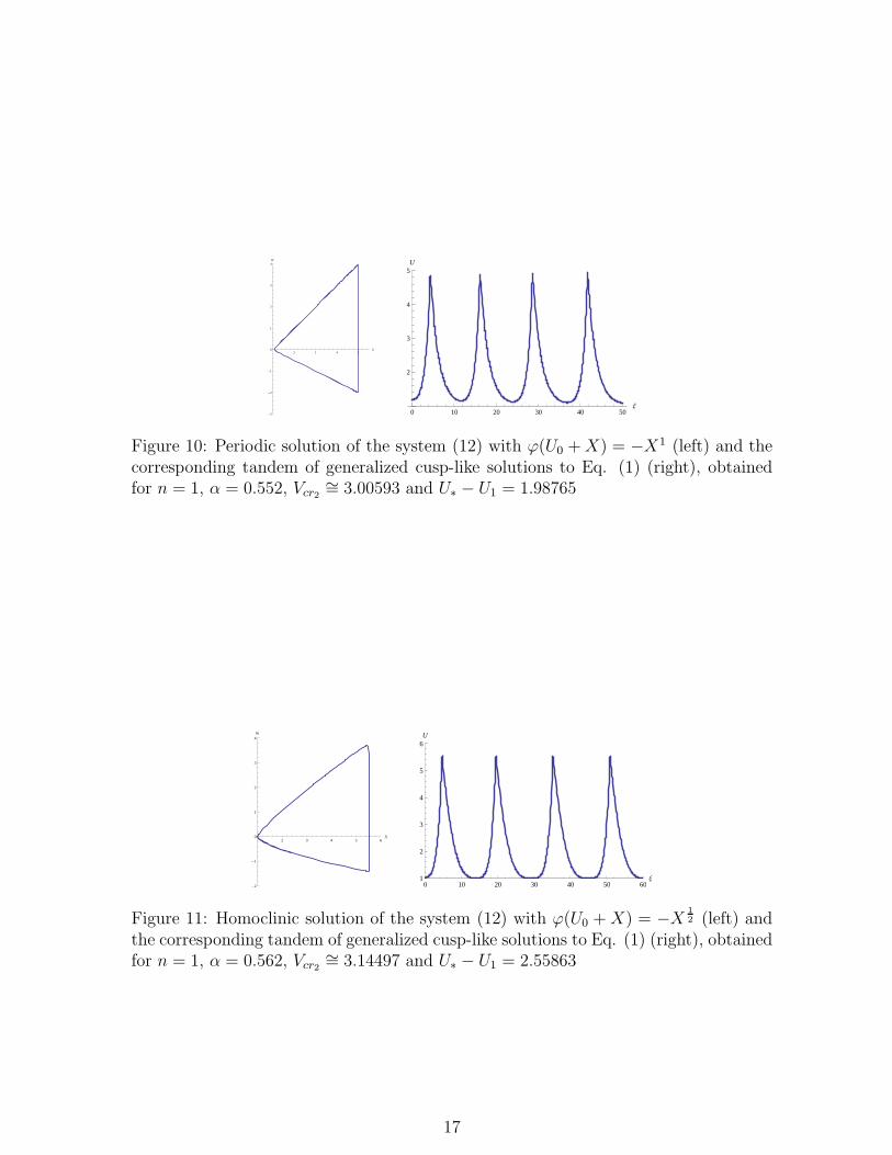
Figure 10: Periodic solution of the system (12) with ϕ(U0 +X) = −X1 (left) and thecorresponding tandem of generalized cusp-like solutions to Eq. (1) (right), obtainedfor n = 1, α = 0.552, Vcr2

∼= 3.00593 and U∗ − U1 = 1.98765

2 3 4 5 6X

-2

-1

0

1

2

3

4W

0 10 20 30 40 50 60Ξ1

2

3

4

5

6U

Figure 11: Homoclinic solution of the system (12) with ϕ(U0 +X) = −X 1

2 (left) andthe corresponding tandem of generalized cusp-like solutions to Eq. (1) (right), obtainedfor n = 1, α = 0.562, Vcr2

∼= 3.14497 and U∗ − U1 = 2.55863

17

periment the function ϕ(U0 + X) = −Xm. Numerical study shows, that the radiusof the limit cycle grows as the bifurcation parameter V grows. Simultaneously thecoordinate U∗(V ) of the singular line intersection with the horizontal axis moves to theright, but not so quickly as the radius of the limit cycle. In most cases the destructionof the periodic trajectory observed was due to its interaction with the line ∆(U) = 0.For m = n = 1 we succeeded in observing how the limit cycle approaches the line ofsingularity, attaining the triangle shape Fig. 10, left. The corresponding succession ofthe cusp-like travelling waves is shown in the right picture. Let us note, that we werenot able to follow the moment of the homoclinic bifurcation, varying the parameters αand V .

Experimenting with m = 1/2, n = 1 occurs to be more easy. The homoclinicbifurcation, shown in the left picture of the Fig.10, takes place when the far end ofthe cycle attains the line ∆(U) = 0. The presence of the singular line causes a drasticchange of the shape of homoclinic loop, which equally well can be called the ”homoclinictriangle”. The right picture shows the corresponding succession of the well-separatedpeakons.

Let us note in conclusion that numerical experiments performed for the paraboliccase, i.e. for α = 0, demonstrate quite similar behavior of the TW and their dependenceupon the parameters (for more details, see [19]).

6 Final remarks

So it was shown in this study, that the generalized convection-reaction-diffusion equa-tion (1) possesses a wide variety of TW solution, such as solitons, compactons, shock-like solutions and peakons. The result of the qualitative analysis and numerical simu-lation are in agreement with each other. The hyperbolic case occurs to be more reach,since the soliton-like solutions and peakons are observed only when α > 0. Surpris-ingly enough, one-sided compactons exist not only when the stationary point lies onthe singular line ∆(U) = 0, but also when it lies left-hand side of it. Condition m > 1assures in the last case the existence of the sharp front.

The results obtained are not rigorous. Only heuristic arguments are attached infavor of the statement that for m 6= 1/2 an infinite ”time” is needed to reach the point(U0, 0), moving along the incoming separatrice of the saddle sector. The precision ofthe numerical method used does not enable us to get convinced that we deal with shockfronts with exponentially localized ”tails” in cases of small m ∈ N+, when the criticalpoint (U0, 0) demonstrates essential instability and the ”trains” of sharply ended pulsesare observed, instead of truly localized solitary waves. More precise description of thewave patterns seems to be possible by presenting them in the form of exponential series[13]. Another possibility is connected with the application of the rigorous computingmethods [23]. Aside of the scope of this study remained the study of stability andattracting properties of the invariant TW solutions. We plan to address these issuesin the forthcoming studies.

18

References

[1] Olver P., Applications of Lie Groups to Differential Equations , Springer–Verlag:New York, Berin, Tokyo, 1996.

[2] Dodd R.K., Eilbek J.C., Gibbon J.D., Morris H.C., Solitons and Nonlinear WaveEquations , Academic Press, London 1984.

[3] W.Ficket, Davis W.C., Detonation, Berkley: Univ. of California Press, 1979.

[4] Rosenau P. and Hyman J., Compactons: Solitons with Finite Wavelength, PhysRev. Letter, vol. 70 (1993), No 5, 564-567.

[5] Li Y.A. and Olver P.J., Convergence of Solitary-Wave Solutions in a Per-turbed Bi-Hamiltonian Dynamical System. 1. Compactons and Peakons , Dis-crete and Continuous Dynamical systems, vol. 3 (1997), pp. 419-432. (see alsohttp://www.math.umn.edu/∼olver)

[6] Li Y.A. and Olver P.J., Rosenau Ph., Non-Analtic Solutions of Nonlinear WaveModels , in: nonl. Theory of Generalized functions, M. grosser, G. Hormann,M. Kunzinger and M. Oberguggenberger, eds., Research Notes in Mathemat-ics, vol. 401, Chapmann and hall/CRC, New York, 1999, pp. 129-145 (see alsohttp://www.math.umn.edu/∼olver).

[7] Vladimirov V., Compacton-like Solutions of the Hydrodynamic System DescribingRelaxing Media , Rep. Math. Phys. 61 (2008), 381-400.

[8] Joseph D.D., Preziozi, L., Heat Waves, Review of Modern Physics, vol. 61, no. 1(1989), 41-73.

[9] Makarenko A.S., New Differential Equation Model for Hydrodynamics with MemryEffects, Reports on Mathematical Physics, vol. 46, No. 1/2 (2000), 183-190.

[10] Makarenko A.S., Moskalkov M., Levkov S., On Blow-up Solutions in Turbulence,Phys Lett., vol. A23 (1997), 391-397.

[11] Kar S., Banik S.K., Ray Sh., Exact Solutions of Fisher and Burgers Equations withFinite Transport Memory, Jornal of Physics A: Mathematical and Theoretical, vol.36, No. 11 (2003), 2771-2780.

[12] Vladimirov V. and Kutafina E., Exact Travelling Wave Solutions of Some Non-linear Evolutionary Equations , Rep. Math. Physics, vol. 54 (2004), 261–271.

[13] Vladimirov V. and Kutafina E.,Pudelko A., Construction Soliton and Kink So-lutions of PDE Models in Transport and Biology, SIGMA, vol. 1 (2005), Paper16.

19

[14] Vladimirov V. and Kutafina E., Analytical Description of the Coherent Structureswithin the Hyperbolic Generalization of Burgers Equation, Rep. Math. Physics,vol.58 (2006), 465.

[15] Vladimirov V. and Maczka Cz., Exact Solutions of Generalized Burgers Equation,Descriing Travelling Fronts and Their Interactions , Rep. Math. Physics, vol. 60(2007), 317-328.

[16] Fahmy E.S., Abdusalam h.A., Raslan K.R., On the Solutions of the Time DelayedBurgers Equation, Nonlinear Analysis, vol. 69 (2008), 4475-4786.

[17] Rosenau P. and Pikovsky A., Phase Compactons in Chains of Dispersively CoupledOscillators, Phys. Rev. Lett., vol. 94 (2005) 174102.

[18] Pikovsky A. and Rosenau P., Phase Compactons, Physica D, vol. 218 (2006)56–69.

[19] Vladimirov V., Maczka Cz., On the Localized Wave Patterns Supported byConvection–Reaction–Diffusion Equation , Rep. Math. Physics, (2009), to appear.

[20] Hassard B., Kazarinoff N., Wan Y.-H., Theory and Applications of Hopf Bifurca-tion, Cambridge Univ. Press: London, New York, 1981.

[21] Guckenheimer J., Holmes P., Nonlinear Oscillations, Dynamical Systems and Bi-furcations of Vector Fields, Springer–Verlag: New York Inc, 1987.

[22] Andronov A., Leontovich E., Gordon I and Meyer A., Qualitative Theory of 2-ndOrder Dynamical Systems, Nauka Publ., Moscow, 1976 (in Russian).

[23] Mishaikov K., Zgliczynski P., Rigorous Numerics for PDEs:the Kuramoto-Sivashinski Equation, Foundations of Computional mathematics, vol. 1 (2001),255-288.

20