Embed Size (px)
Citation preview

Research Institute for Advanced Computer ScienceNASA Ames Research Center
/,,v-_¢,'/
3D
SPARSKIT" a basic tool kit for
sparse matrix computations(NA_A-CR-135_76) 5PARSKIT: A E_A_IC TOSL KIT
FqR SPARS_ MAT_I× C_HPUTATIONS (Oese3rch
Inst. for Adv_nc_d Computer $ciAnce) 30 pC_CL 12A
Ngl-3Z_65
Unclds
83/04 O0_3046
Youcef Saad
RIACS Technical Report 90.20
https://ntrs.nasa.gov/search.jsp?R=19910023551 2018-06-13T08:51:33+00:00Z

_kJ_i !
i
SPARSKIT: a basic tool kit for
sparse matrix computations
Youcef Saad
. _ _o° -% °. o "'-_#*
The Research Institute for Advanced Computer Science is operated by Universities Space Research
Association (USRA), The American City Building, Suite 311, Columbia, MD 21044, (301)730-2656.
Work reported herein was supported in part by DARPA via Cooperative Agreement NCC 2-387 between
NASA and USRA.


SPARSKIT: a basic tool kit for
sparse matrix computations
Youcef Saad*
May _I, 1990
Abstract. This paper presents the main features of a tool package for manipulating and working
with sparse matrices. One of the goals of the package is to provide basic tools to facilitate exchangeof software and data between researchers in sparse matrix computations. Our starting point is the
Harwell/Boeing collection of matrices for which we provide a number of tools. Among other things
the package provides programs for converting data structures, printing simple statistics on a matrix,
plotting a matrix profile, performing basic linear algebra operations with sparse matrices and so on.
*RIACS, Mail Stop 230-5, NASA Ames Research Center, Moffett Field, CA 94035. This work was
supported in part by the NAS Systems Division, via Cooperative Agreement NCC 2-387 between NASA
and the University Space Research Association (USRA) and in part by the Department of Energy under
grant DE-FG02-85ER25001.

SPARSKIT 2
1 Introduction
Research on sparse matrix techniques has become increasingly complex, and this trend is
likely to accentuate if only because of the growing need to design efficient sparse matrix
algorithms for modern supercomputers. While there are a number of packages and 'user
friendly' tools, for performing computations with small dense matrices there is a lack
of any similar tool or in fact of any common tools for working with sparse matrices.
Yet a collection of a few basic programs to perform some elementary and common tasks
may be very useful in reducing the typical time to implement and test sparse matrix
algorithms. That a common set of routines shared among researchers does not exist yet
for sparse matrix computation is rather surprising. Consider the contrasting situation
in dense matrix computations. The Linpack and Eispack packages developed in the
70's have been of tremendous help in various areas of scientific computing. One could
speculate that the widespread availability of these packages must have saved millions
of hours of coding effort world-wide. In contrast, it is very common that researchers in
sparse matrix computation code their own subroutine for such things as converting the
storage mode of a matrix or for reordering a matrix according to a certain permutation.
One of the reasons for this situation might be the absence of any standard for sparse
matrix computations. For instance, the number of different data structures used to store
sparse matrices in various applications is staggering. For the same basic data structure
there often exist a large number of variations in use. As sparse matrix computation
technology is maturing there is a desperate need for some standard for the basic storage
schemes and possibly, although this is more controversial, for the basic linear algebra
operations.
An important example where a package such as SPARSKIT can be helpful is for
exchanging matrices for research or other purposes. In this situation, one must often
translate the matrix from some initial data structure in which it is generated, into a
different desired data structure. One way around this difficulty is to restrict the number
of schemes that can be used and set some standards. However, this is not enough
because often the data structures are chosen for their efficiency and convenience, and it
is not reasonable to ask practitioners to abandon their favorite storage schemes. What
is needed is a large set of programs to translate one data structure into another. In the
same vein, subroutines that generate test matrices would be extremely valuable since
they would allow users to have access to a large number of matrices without the burden
of actually passing large sets of data.
A useful collection of sparse matrices known as the Harwell/Boeing collection, which
is publically available [4], has been widely used in recent years for testing and comparison
purposes. Because of the importance of this collection many of the tools in SPARSKIT
can be considered as companion tools to it. For example, SPARSKIT supplies simple
routines to create a Harwell/Boeing (H/B) file from a matrix in any format, tools for
creating pic files in order to plot a H/B matrix, a few routines that will deliver statistics
for any H/B matrix, etc.. However, SPARSKIT is not limited to being a set of tools
to work with H/B matrices. Since one of our main motivations is research on iterative

SPARSKIT 3
methods, we provide numerous tools that may help researchers in this specific area.
SPARSKIT will hopefully be an evolving package that will benefit from contributions
from other researchers. This report is a succinct description of the package in its version
one release.
2 Data structures for sparse matrices and the con-
version routines
One of the dimculties in sparse matrix computations is the variety of types of matrices
that are encountered in practical applications. The purpose of each of these schemes is
to gain efficiency both in terms of memory utilization and arithmetic operations. As a
result many different ways of storing sparse matrices have been devised to take advantage
of the structure of the matrices or the specificity of the problem from which they arise.
For example if it is known that a matrix consists of a few diagonals one may simply
store these diagonals as vectors and the offsets of each diagonal with respect to the main
diagonal. If the matrix is not regularly structured, then one of the most common storage
schemes in use today is what we refer to in SARSKIT as the Compressed Sparse Row
(CSR) scheme. In this scheme all the nonzero entries are stored one row after the other
in a one-dimensional real array A together with an array JA containing their column
indices and a pointer array which contains the addresses in A and JA of the beginning of
each row. A]so of importance because of its simplicity is the coordinate storage scheme
in which the nonzero entries of A are stored in any order together with their row and
column indices. Many of the other existing schemes are specialized to some extent. The
reader is referred to the book by Duff et al. [3] for more details.
2.1 Storage Formats
Currently, the conversion routines of SPARSKIT can handle twelve different storage
formats. These include some of the most commonly used schemes but they are by no
means exhaustive. We found it particularly useful to have all these storage modes when
trying to extract a matrix from someone else's application code in order, for example,
to analyze it with the tools described in the next sections or, more commonly, to try a
given solution method which requires a different data structure than the one originally
used in the application. Often the matrix is stored in one of these modes or a variant
that is very close to it. We hope to add many more conversion routines as SPARSKIT
evolves.
In this section we describe in detail the storage schemes that are handled in the
FORMATS module. For convenience we have decided to label by a three character name
each format used. We start by listing the formats and then describe them in detail in
separate subsections (except for the dense format which needs no detailed description).
DNS Dense format
SPARSKIT 4
BND Linpack Banded format
CSR Compressed Sparse Row format
CSC Compressed Sparse Column format
CO0 Coordinate format
ELL Ellpack-Itpack generalized diagonal format
DIA Diagonal format
BaR Block Sparse Row format
MSR Modified Compressed Sparse Row format
SSK Symmetric Skyline format
NSK Nonsymmetric Skyline format
JAD The Jagged Diagonal scheme
In the following sections we denote by A the matrix under consideration and by N
its row dimension and NNZ the number of its nonzero elements.
2.1.1 The Compressed Sparse Row and related formats (CSR, CSC and
MSR)
The Compressed Sparse Row format is the basic format used in SPARSKIT. The data
structure for Compressed Sparse Row consists of three arrays.
• A real array A containing the real values alj stored row by row, from row 1 to N.
The length of A is NNZ.
• An integer array JA containing the column indices of the elements alj as stored
in the array A. The length of JA is NNZ.
• An integer array IA containing the pointers to the beginning of each row in the
arrays A and JA. Thus the content of IA(i) is the position in arrays A and JA
where the i-th row starts. The length of IA is N -k 1 with IA(N q- 1) containing
the number IA(1) q- NNZ, i.e., the address in A and JA of the beginning of a
fictitious row N + 1.
The Compressed Sparse Column format is identical with the Compressed Sparse Row
format except that the columns of A are stored instead of the rows. In other words the
Compressed Sparse Column format is simply the Compressed Sparse Row format for the
matrix A r.

SPARSKIT 5
The Modified Sparse Row (MSR) format is a rather common variation of the Com-
pressed Sparse Row format which consists of keeping the main diagonal of A separately.
The corresponding data structure consists of a real array A and an integer array JA.
The first N positions in A contain the diagonal elements of the matrix, in order. The
position N + 1 of the array A is not used. Starting from position N + 2, the nonzero
elements of A, excluding its diagonal elements, are stored row-wise. Corresponding to
each element A(k) the integer JA(k) is the column index of the element A(k) in the
matrix A. The N + 1 first positions of JA contain the pointer to the beginning of each
row in A and JA. The advantage of this storage mode is that many matrices have a
full main diagonal, i.e., a_i _ O,i = 1,... ,N, and this diagonal is best represented by
an array of length N. This storage mode is particularly useful for triangular matrices
with non-unit diagonals. Often the diagonal is then stored in inverted form (i.e. 1/aii
is stored in place of ali) because triangular systems are often solved repeatedly with the
same matrix many times, as is the case for example in preconditioned Conjugate Gra-
dient methods. The column oriented analogue of the MSR format, called MSC format,
is also used in some of the other modules, but no transformation to/from it to the CSC
format is necessary: for example to pass from CSC to MSC one can use the routine to
pass from the CSR to the MSR formats, since the data structures are identical. The
above three storage modes are used in many well-known packages.
2.1.2 The banded Linpack format (BND)
Banded matrices represent the simplest form of sparse matrices and they often convey
the easiest way of exploiting sparsity. There are many ways of storing a banded matrix.
The one we adopted here follows the data structure used in the Linpack banded solution
routines. The motivation here is that one can often make use of this well-known package
if the matrices are banded. For fairly small matrices (say, N < 2000 on supercomputers,
N < 200 on fast workstations, and with a bandwidth of O(N½)), this may represent
a viable and simple way of solving linear systems. One must first transform the initial
data structure into the banded linpack format and then call the appropriate band solver.
For large problems it is clear that a better alternative would be to use a sparse solver
such as MA28, which requires the input matrix to be in the coordinate format.
In the BND format the nonzero elements of A are stored in a rectangular array ABD
with the nonzero elements of the j-th column being stored in the j - th column of
ABD. We also need to know the number ML of diagonals below the main diagonals
and the number MU of diagonals above the main diagonals. Thus the bandwidth of A
is ML + MU + 1 which is the minimum number of rows required in the array ABD.
An additional integer parameter is needed to indicate which row of ABD contains the
lowest diagonal.
2.1.3 The coordinate format (COO)
The coordinate format is certainly the simplest storage scheme for sparse matrices. It
consists of three arrays: a real array of size NNZ containing the real values of nonzero

SPARSKIT 6
elements of A in any order, an integer array containing their row indices and a second
integer array containing their column indices. Note that this scheme is as general as the
CSR format, but from the point of view of memory requirement it is not as efficient.
On the other hand it is attractive because of its simplicity and the fact that it is very
commonly used. Incidentally, we should mention a variation to this mode which is
perhaps the most economical in terms of memory usage. The modified version requires
only a real array A containing the real values a_j along with only one integer array that
contains the integer values (i- 1)N +j for each corresponding nonzero element alj. It is
clear that this is an unambiguous representation of all the nonzero elements of A. There
are two drawbacks to this scheme. First, it requires some integer arithmetic to extract
the column and row indices of each element when they are needed. Second, for large
matrices it may lead to integer overflow because of the need to deal with integers which
may be very large (of the order of N2). Because of these two drawbacks this scheme has
seldom been used in practice.
2.1.4 The diagonal format (DIA)
The matrices that arise in many applications often consist of a few diagonals. This
structure has probably been the first one to be exploited for the purpose of improving
performance of matrix by vector products on supercomputers, see references in [8]. To
store these matrices we may store the diagonals in a rectangular array DIAG(1 : N, 1 :
NDIAG) where NDIAG is the number of diagonals. We also need to know the offsets
of each of the diagonals with respect to the main diagonal. These will be stored in an
array IOFF(1 : NDIAG). Thus, in position (i,/_) of the array DIAG is located the
element ai,_+_oyy(k) of the original matrix. The order in which the diagonals are stored in
the columns of DIAG is unimportant. Note also that all the diagonals except the main
diagonal have fewer than N elements, so there are positions in DIAG that will not be
used.
In many applications there is a small number of non-empty diagonals and this scheme
is enough. In general however, it may be desirable to complement this data structure,
e.g., by a compressed sparse row format. A general matrix is therefore represented as
the sum of a diagonal-structured matrix and a general sparse matrix. The conversion
routine CSRDIA which converts from the compressed sparse row format to the diagonal
format has an option to this effect. If the user wants to convert a general sparse matrix
to one with, say, 5 diagonals, and if the input matrix has more than 5 diagonals, the rest
of the matrix (after extraction of the 5 desired diagonals) will be put, if desired, into a
matrix in the CSR format. In addition, the code may also compute the most important
5 diagonals if wanted, or it can get those indicated by the user through the array IOFF.
2.1.5 The Ellpack-Itpack format (ELL)
The Ellpack-Itpack format [6, 9, 5] is a generalization of the diagonal storage scheme
which is intended for general sparse matrices with a limited maximum number of nonze-
ros per row. Two rectangular arrays of the same size are required, one real and one

SPARSKIT 7
integer. The first, COEF, is similar to DIAG and contains the nonzero elements of
A. Assuming that there are at most NDIAG nonzero elements in each row of A,
we can store the nonzero elements of each row of the matrix in a row of the array
COEF(1 : N, 1 : NDIAG) completing the row by zeros if necessary. Together with
COEF we need to store an integer array JCOEF(1 : N, 1 : NDIAG) which contains
the column positions of each entry in COEF.
2.1.6 The Block Sparse Row format (BSR)
Block matrices are common in all areas of scientific computing. The best way to describe
a block matrix is by saying that it is a sparse matrix whose nonzero entries are square
dense blocks. Block matrices arise from the discretization of partial differential equations
when there are several degrees of freedom per grid point. There are restrictions to thisscheme. Each of the blocks is treated as a dense block. If there are zero elements within
each block they must be treated as nonzero elements with the value zero.
There are several variations to the method used for storing sparse matrices with
block structure. The one considered here, the Block Sparse Row format, is a simple
generalization of the Compressed Sparse Row format.
We denote here by NBLK the dimension of each block, by NNZR the number of
nonzero blocks in A (i.e., NNZR - NNZ/(NBLK')) and by NR the block dimension
of A, (i.e., NR = N/NBLK), the letter R standing for 'reduced'. Like the Compressed
Sparse Row format we need three arrays. A rectangular real array A(1 : NNZR, 1 :
NBLK, 1 : NBLK) contains the nonzero blocks listed (block)-row-wise. Associated
with this real array is an integer array JA(1 : NNZR) which holds the actual column
positions in the original matrix of the (1,1) dements of the nonzero blocks. Finally, the
pointer array IA(1 : NR + 1) points to the beginning of each block row in A and JA.
The savings in memory and in the use of indirect addressing with this scheme over
Compressed Sparse Row can be substantial for large values of NBLK.
2.1.7 The Symmetric Skyline format (SSK)
A Skyline matrix is often referred to as a variable band matrix or a profile matrix [3].
The main attraction of skyline matrices is that when pivoting is not necessary then the
skyline structure of the matrix is preserved during Ganssian elimination. If the matrix
is symmetric we need only to store its lower triangular part. This is a collection of rows
whose length varies. A simple method used to store a Symmetric Skyline matrix is to
place all the rows in order from 1 to N, [2] in a real array A and then keep an integer
array which holds the pointers to the beginning of each row. The column positions of
the nonzero elements stored in A can be easily derived and are therefore not kept.
2.1.8 The Non Symmetric Skyline format (NSK)
Conceptually, the data structure of a nonsymmetric skyline matrix consists of two sub-
structures. The first consists of its lower part of A stored in skyline format and the
_;PARSKIT 8
second of its upper triangular part stored in a column oriented skyline format (i.e., the
transpose is stored in standard row skyline mode). Several ways of putting these sub-
structures together may be used and there are no compelling reasons for preferring one
strategy over another one. We chose to store contiguously each row of the lower part
and column of the upper part of the matrix. The real array A will contain the 1-st row
followed by the first column (empty), followed by the second row followed by the second
column, etc.. An additional pointer is needed to indicate where the diagonal elements,
which separate the lower from the upper part, are located in this array.
2.1.9 The Jagged Diagonal Format (JAD)
This storage mode is very useful for the efficient implementation of iterative methods
on parallel and vector processors [8]. Starting from the CSR format, the idea is to first
reorder the rows of the matrix decreasingly according to their number of nonzeros entries.
Then, a new data structure is built by constructing what we call "jagged diagonals" (j-
diagonals). We store as a dense vector, the vector consisting of all the first elements in
A, JA from each row, together with an integer vector containing the column positions of
the corresponding elements. This is followed by the second jagged diagonal consisting of
the elements in the second positions from the left. As we build more and more of these
diagonals, their length decreases. The number of j-diagonals is equal to the number of
nonzero elements of the first row, i.e., to the largest number of nonzero elements per row.
The data structure to represent a general matrix in this form consists, before anything,
of the permutation array which reorders the rows. Then the real array A containing the
jagged diagonals in succession and the array JA of the corresponding column positions
are stored, together with a pointer array IA which points to the beginning of each jagged
diagonal in the arrays A, JA. The advantage of this scheme for matrix multiplications
has been illustrated in [8] and in [1] in the context of triangular system solutions.
2.2 The FORMATS conversion module
It is important to note that there is no need to have a subroutine for each pair of data
structures, since all we need is to be able to convert any format to the standard row-
compressed format and then back to any other format. There are currently 23 different
conversion routines in this module all of which are devoted to converting from one date
structure to another.
The naming mechanism adopted is to use a 6-character name for each of the sub-
routines the first 3 for the input format and the last 3 for the output format. Thus
COOCSR does the conversion from the coordinate format to the Compressed Sparse
Row format. However it was necessary to break the naming rule in one exception. We
needed a version of COOCSR that is in-place, i.e., which can take the input matrix, and
convert it directly into a CSR format by using very little additional work space. This
routine is called COICSR. Each of the formats has a routine to translate it to the CSR
format and a routine to convert back to it from the CSR format. The only exception
is that a CSCCSR routine is not necessary since the conversion from Column Sparse
SPARSKIT 9
format to Sparse Row format can be performed with the same routine CSRCSC. This
is essentially a transposition operation.
Considerable effort has been put in attempting to make the conversion routines in-
place, i.e., in allowing some or all of the output arrays to be the same as the input arrays.
The purpose is to save storage whenever possible without sacrificing performance. The
added flexibility can be very convenient in some situations. When the additional coding
complexity to permit the routine to be in place was not too high this was always done.
If the subroutine is in-place this is clearly indicated in the documentation. There is one
case where we found it necessary to provide the in-place version as well as the regular
version: COICSR is an in-place version of the COOCSR routine. We would also like
to add that other routines that avoid the CSR format for some of the more important
data structures may eventually be included. For now, there is only one such routine 1
namely, COOELL.
2.3 Internal format used in SPARSKIT
Most of the routines in SPARSKIT use internally the Compressed Sparse Row format.
The selection of the CSR mode has been motivated by several factors. Simplicity, gener-
ality, and widespread use are certainly the most important ones. However, it has often
been argued that the column scheme may have been a better choice. One argument in
this favor is that vector machines usually give a better performance for such operations
as matrix vector by multiplications for matrices stored in CSC format. In fact for paral-
lel machines which have a low overhead in loop synchronization (e.g., the Alliants), the
situation is reversed, see [8] for details. For almost any argument in favor of one scheme
there seems to be an argument in favor of the other. Fortunately, the difference provided
in functionality is rather minor. For example the subroutine APLB to add two matrices
in CSR format, described in Section 5.1, can actually be also used to add two matrices
in CSC format, since the data structures are identical. Several such subroutines can be
used for both schemes, by pretending that the input matrices are stored in CSR mode
whereas in fact they are stored in CSC mode.
3 Manipulation routines
The module UNARY of SPARSKIT consists of a number of utilities to manipulate and
perform basic operations with sparse matrices. The following sections give an overview
of this part of the package.
3.1 Miscellaneous operations with sparse matrices
There are a large number of non-algebraic operations that are commonly used when
working with sparse matrices. A typical example is to transform A into B = PAQ
1Contributed by E. Rothman from Corner University.

SPARSKIT 10
where P and Q are two permutation matrices. Another example is to extract the lower
triangular part of A or a given diagonal from A. Several other such 'extraction' opera-
tions are supplied in SPARSKIT. Also provided is the transposition function. This may
seem as an unnecessary addition since the routine CSRCSC already does perform this
function economically. However, the new transposition provided is in place, in that it
may transpose the matrix and overwrite the result on the original matrix, thus saving
memory usage. Since many of these manipulation routines involve one matrix (as op-
posed to two in the basic linear algebra routines) we created a module called UNARY
to include these subroutines.
Another set of subroutines that are sometimes useful are those involving a 'mask'.
A mask defines a given nonzero pattern and for all practical purposes a mask matrix is
a sparse matrix whose nonzero entries are all ones (therefore there is no need to store
its real values). Sometimes it is useful to extract from a given matrix A the 'masked'
matrix according to a mask M, i.e., to compute the matrix A ® M , where ® denotes
the element-wise matrix product, and M is some mask matrix.
3.2 The module UNARY
This module of SPARSKIT consists of a number of routines to perform some basic
non-algebraic operations on a matrix. The following is a list of the routines currently
supported with a brief explanation.
SUBMAT
FILTER
TRANSP
COPMAT
GETDIA
Extracts a square or rectangular submatrix from a sparse matrix.
The input is a matrix in CSR format the output is a matrix in
CSR format. The output matrix can, if desired, be overwritten
on the input matrix (Algorithm is "in place").
Filters out elements from a matrix according to their magnitude.
The input is a matrix in CSR format, the output is a matrix in
CSR format, obtained from the input matrix by removing all its
elements that are smaller than a certain threshold. The thresh-
old is computed for each row according to one of three provided
options. The algorithm is in place.
This is an in-place transposition routine, i.e., it is an in place
version of the CSRCSC routine in FORMATS.
Copy of a matrix into another matrix (both stored CSR).
Extracts a specified diagonal from a matrix. An option is provided
to transform the input matrix so that the diagonal is removed from
its entries. Otherwise the diagonal is extracted and the input
matrix remains untouched.

SPARSKIT 11
GETL
GETU
LEVELS
AMASK
CPERM
RPERM
DPERM
VPERM
RETMX
DIAPOS
EXTBDG
GETBWD
BLKFND
BLKCHK
This subroutine extracts the lower triangular part of a matrix,
including the main diagonal. The algorithm is in-place.
Extracts the upper triangular part of a matrix. Similar to GETL.
Computes the level scheduling data structure for lower triangular
matrices, see [1].
Extracts C = A ® M, i.e., performs the mask operation. This
routine computes a sparse matrix from an input matrix A by ex-
tracting only the elements in A, where the corresponding elements
of M are nonzero. The mask matrix M, is a sparse matrix in CSR
format without the real values, i.e., only the integer arrays JM
and IM are of the CSR format are passed.
Permutes the columns of a matrix, i.e., computes the matrix B =
AQ where Q is a permutation matrix.
Permutes the rows of a matrix, i.e., computes the matrix B = PA
where P is a permutation matrix.
Permutes the rows and columns of a matrix, i.e., computes B =
PAQ given two permutation matrices P and Q. This routine
gives a special treatment to the common case where Q = pT.
Performs an in-place permutation of a vector, i.e., performs z :=
Pz, where P is a permutation matrix.
Returns the maximum absolute value in each row of an input
matrix.
Returns the positions in the arrays A and JA of the diagonal
elements, for a matrix stored in CSR format.
Extracts the main diagonal blocks of a matrix.
Returns bandwidth=information on a matrix. This subroutine
returns the bandwidth of the lower part and the upper part of a
given matrix. May be used to determine these two parameters for
converting a matrix into the BND format.
Attempts to find the block-size of a matrix.
Checks whether a given integer is the block size of A. This routine
is called by BLKFND.

SPARSKIT 12
INFDIA Computes the number of nonzero dements of each of the 2n - 1
diagonals of a matrix. (The first diagonal is the diagonal with off-
set -n which consists of the entry a.,1 and the last is the diagonal
with offset n).
AATDGR Computes the number of nonzero elements in each row of thematrix AA r.
ATADGR Computes the number of nonzero elements in each row of thematrix A r A.
APBDGR Computes the number of nonzero elements in each row of the
matrix A + B, given two matrices A and B.
RNRMS Computes the norms of the rows of a matrix. The usual three
normsI1-111,I1-11 ,and I1.11 are supported.
CNRMS Computes the norms of the columns of a matrix. Similar to RN-
RMS.
RSCAL Scales the rows of a matrix by their norms. The same three norms
as in RNRMS are available.
CSCAL Scales the columns of a matrix by their norms. The same three
norms as in RNRMS are available.
4 Input/Output routines
The INOUT module of SPARSKIT comprises a few routines for reading, writing, and for
plotting and visualizing the structure of sparse matrices. These routines are essentially
geared towards the utilization of the Harwell/Boeing collection of matrices. There are
currently only three subroutines in this module.
READMT
PRTMT
PLTG
Reads a matrix in the Harwell/Boeing format.
Creates a Harwell Boeing file from an arbitrary matrix in CSC or
CSC format.
Creates a pic file for plotting the pattern of a matrix.
The routines readmt and prtmt allow to read and create files containing matrices
stored in the H/B format. For details concerning this format the reader is referred to

SPARSKIT I_
[4]. While the purpose of readmt is dear, it is not obvious that one single subroutine
can write a matrix in H/B format and still satisfy the needs of all users. For example for
some matrices all nonzero entries are actually integers and a format using say a 10 digit
mantissa may entail an enormous waste of storage if the matrix is large. The solution
provided is to compute internally the best formats for the integer arrays IA and JA.
A little help is required from the user for the real values in the arrays A and RHS.
Specifically, the desired format is obtained from a parameter of the subroutine by using
a simple notation, see documentation for details.
We found it extremely useful to be able to visualize a sparse matrix, notably for
debugging purposes. A simple look at the plot can sometimes reveal whether the matrix
obtained from some reordering technique does indeed have the expected structure. For
now two simple plotting mechanisms are provided. First, a preprocessor to the Unix
utility 'Pic' allows one to generate a pic file from a matrix that is in the Harwell/Boeing
format or any other format. For example for a Harwell/Boeing matrix file, the commandis of the form
PltMat < HB filename
The output file is then printed by the usual troff or TeX commands. A translation of this
routine into one that generates a post-script file is also available in the module UNSUPP
(see Section 8). We should point out that the plotting routines are very simple in nature
and should not be used to plot large matrices. For example the pltmt routine outputs
one pie command line for every nonzero element. This constitutes a convenient tool for
document preparation for example. Matrices of size just up to a few thousands eva be
printed this way. Several options concerning size of the plot and caption generation areavailable.
Another set of utilities for viewing profiles of sparse matrices on Sun screens is also
available, see Section 8.
5 Basic algebraic operations
The usual algebraic operations involving two matrices, such as C = A+ B, C = A +fiB,
C = AB, etc.., are fairly common in sparse matrix computations. These basic matrix
operations are included in the module called BLASSM. In addition there are a large
number of basic operations, involving a sparse matrix and a vector, such as matrix-vector
products and triangular system solutions that are very commonly used. Some of these
are included in the module MATVEC. Sometimes it is desirable to compute the patterns
of the matrices A + B and AB, or in fact of any result of the basic algebraic operations.
This can be implemented by way of job options which will determine whether to fill-in
the real values or not during the computation. We now briefly describe the contents of
each of the two modules BLASSM and MATVEC.
SPARSKIT 14
5.1 The BLASSM module
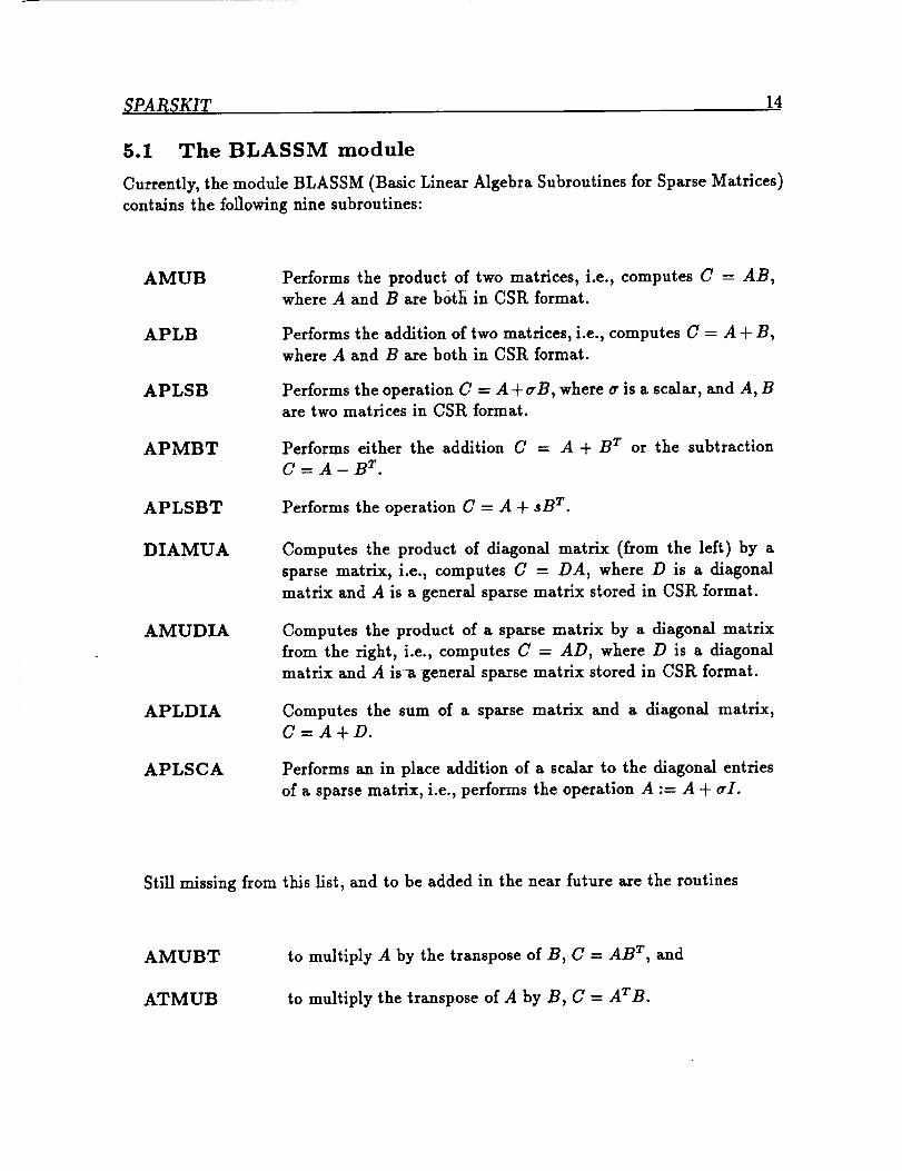
Currently, the module BLASSM (Basic Linear Algebra Subroutines for Sparse Matrices)
contains the following nine subroutines:
AMUB
APLB
APLSB
APMBT
APLSBT
DIAMUA
AMUDIA
APLDIA
APLSCA
Performs the product of two matrices, i.e., computes C = AB,where A and B are both in CSR format.
Performs the addition of two matrices, i.e., computes C = A + B,
where A and B are both in CSR format.
Performs the operation C = A+aB, where tr is a scalar, and A, B
are two matrices in CSR format.
Performs either the addition C = A + B T or the subtraction
C= A-B T.
Performs the operation C = A + sB T.
Computes the product of diagonal matrix (from the left) by a
sparse matrix, i.e., computes C = DA, where D is a diagonal
matrix and A is a general sparse matrix stored in CSR format.
Computes the product of a sparse matrix by a diagonal matrix
from the right, i.e., computes C = AD, where D is a diagonal
matrix and A is a general sparse matrix stored in CSR format.
Computes the sum of a sparse matrix and a diagonal matrix,
C=A+D.
Performs an in place addition of a scalar to the diagonal entries
of a sparse matrix, i.e., performs the operation A := A + aI.
Still missing from this list, and to be added in the near future are the routines
AMUBT
ATMUB
to multiply A by the transpose of B, C = AB T, and
to multiply the transpose of A by B, C = ATB.
SPARSKIT I_
Operations of the form tA ÷ 8B have been avoided as their occurrence does notwarrant additional subroutines. Several other operations similar to those defined for
vectors have not been included. For example the scaling of a matrix in sparse format is
simply a scaling of its real array A, which can be done with the usual BLAS1 scaling
routine, on the array A.
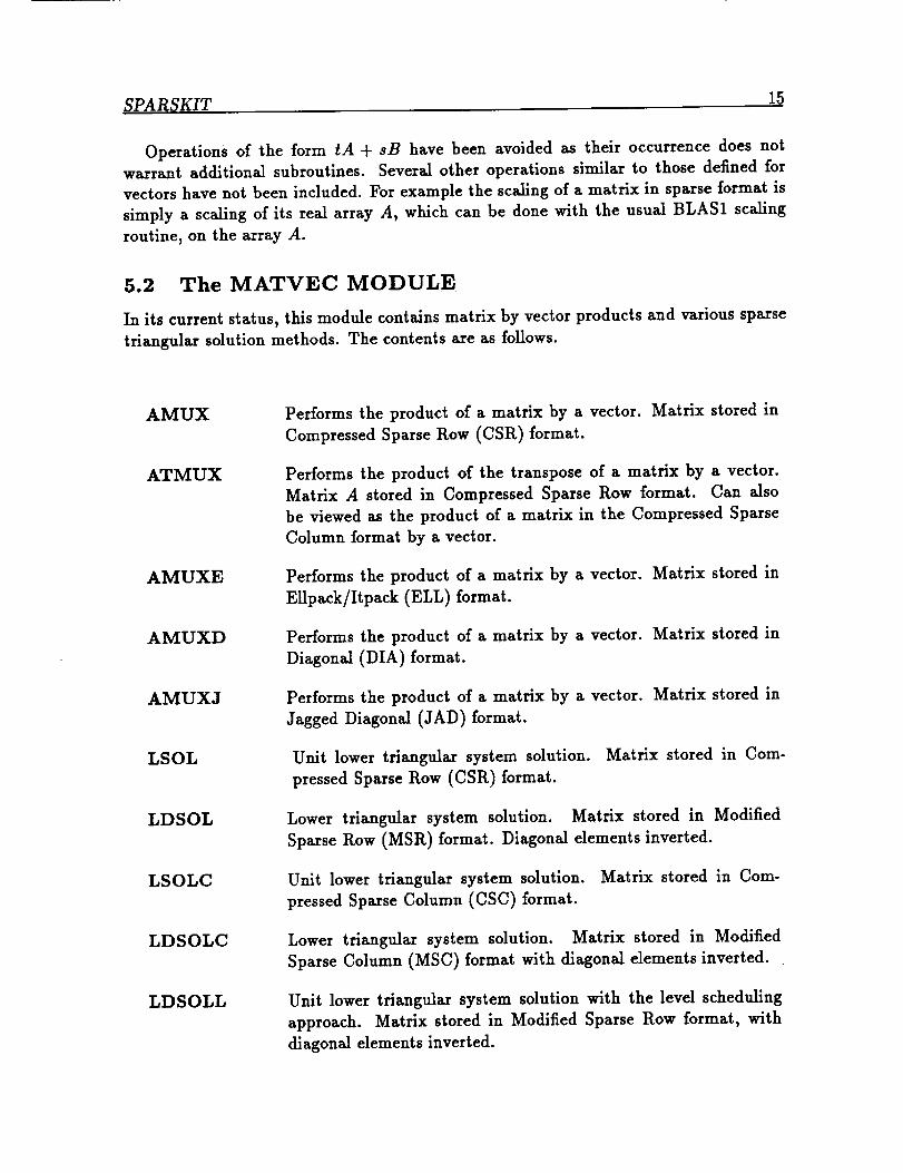
5.2 The MATVEC MODULE
In its current status, this module contains matrix by vector products and various sparse
triangular solution methods. The contents are as follows.
AMUX
ATMUX
AMUXE
AMUXD
AMUXJ
LSOL
LDSOL
LSOLC
LDSOLC
LDSOLL
Performs the product of a matrix by a vector. Matrix stored in
Compressed Sparse Row (CSR) format.
Performs the product of the transpose of a matrix by a vector.
Matrix A stored in Compressed Sparse Row format. Can also
be viewed as the product of a matrix in the Compressed Sparse
Column format by a vector.
Performs the product of a matrix by a vector. Matrix stored in
EUpack/Itpack (ELL) format.
Performs the product of a matrix by a vector. Matrix stored in
Diagonal (DIA) format.
Performs the product of a matrix by a vector. Matrix stored in
Jagged Diagonal (JAD) format.
Unit lower triangular system solution. Matrix stored in Com-
pressed Sparse Row (CSR) format.
Lower triangular system solution. Matrix stored in Modified
Sparse Row (MSR) format. Diagonal elements inverted.
Unit lower triangular system solution. Matrix stored in Com-
pressed Sparse Column (CSC) format.
Lower triangular system solution. Matrix stored in Modified
Sparse Column (MSC) format with diagonal elements inverted.
Unit lower triangular system solution with the level scheduling
approach. Matrix stored in Modified Sparse Row format, with
diagonal elements inverted.

_PARSKIT 16
USOL
UDSOL
USOLC
UDSOLC
Unit upper triangular system solution. Matrix stored in Com-
pressed Sparse Row (CSR) format.
Upper triangular system solution. Matrix stored in Modified
Sparse Row (MSR) format. Diagonal elements inverted.
Unit upper triangular system solution. Matrix stored in Com-
pressed Sparse Column (CSC) format.
Upper triangular system solution. Matrix stored in Modified
Sparse Column (MSC) format with diagonal elements inverted.
Most of the above routines are very short and rather straightforward. A long test
program is provided to run all of the subroutines on a large number of matrices that are
dynamically generated using the MATGEN module.
6 The basic statistics and information routines
It is sometimes very informative when analyzing solution methods, to be able in a short
amount of time to obtain some statistical information about a sparse matrix. The
purpose of the subroutine infol, is to print out such information. The question we
had to address at first was to determine what type of information was the most useful
without being too expensive to obtain. The simplest and most common statistics are:
total number of nonzero elements, average number of nonzero elements per row (with
standard deviation), band size. Our preliminary package Infol contains the above and a
number of other features. For example it answers the following questions: Is the matrix
lower triangular, upper triangular? does it have a symmetric structure? If not how
close is it from having this property? Is it weakly row-diagonally dominant? What
percentage of the rows are weakly diagonally dominant? Same questions for column
diagonal dominance. A sample output from infol is listed in Figure1. This print-out
was generated by typing
infol _ pores_2
where pores_2 is a file containing a matrix in H/B format.
If the Harwell-Boeing matrix is symmetric then Infol takes this information into ac-
count to obtain the correct information instead of the information on the lower triangular
part only. Moreover, in cases where only the pattern is provided (no real values), then
infol will print a message to this effect and will then give information related only to the
structure of the matrix. The output for an example of this type is shown in Figure 2.
We should point out that the runs for these two tests were basically instantaneous on a
Sun-4 workstation.

SPARSKIT 17
* Dimension N
* Number of nonzero elements
* Average number of nonzero elements/Column
* Standard deviation for above average
* Nonzero elements in strict upper part
* Nonzero elements in strict lower part
* Nonzero elements in main diagonal
* Weight of longest column
* Weight of shortest column
* Weight of longest row
* Weight of shortest row
* Matching elements in symmetry
* Relative Symmetry Match (symmetry=l)
* Average distance of a(i,j) from diag.
* Standard deviation for above average
= 1224 *
= 9613 *
= 7.8538 *
5.4337 *
= 4384 *
= 4005 *
= 1224 *
= 30 *
= 2 *
= 30 *
= 2 *
= 6358 *
= 0.6614 *
= 0.615E+02 *
= 0.103E+03 *
* Frobenius norm of A
* Frobenius norm of symmetric part
* Frobenius norm of nonsymmetric part
* Maximum element in A
* Percentage of weakly diagonally dominant rows
_e
Percentage of weakly diagonally dominant columns =
0.150E+09 *
0.100E+09 *
0.951E+08 *
0.378E+08 *
0.481E+00 *
0.490E-02 *
* Lower bandwidth (max: i-j, a(i,j) .ne. O)
* Upper bandwidth (max: j-i, a(i,j) .he. O)
* Maximum Bandwidth
* Average Bandwidth
* Number of nonzeros in skyline storage
* 90_ of matrix is in the band of width
* 80g of matrix is in the band of width
* The total number of nonvoid diagonals is
* The I0 most important diagonals are (offsets)
* 0 I -1 -2 2 -3 -32 -264
* The accumulated percentages they represent are
* 12.7 24.6 31.7 37.9 43.6 49.0 52.4 55.7
= 470 *
= 471 *
= 736 *
= 0.190E+03 *
= 340385 *
= 527 *
= 145 *
= 367 *
: *
264 32 *
58.6 61.4 *
The matrix does not have a block structure
Figure 1: Sample output from Infol

SPARSKIT 18
**************************************
• SYMMETRIC PATTERN FROM CANNES ,LUCIE_ MARR0, JUNE 1981. *
• Key = CAN 1072 , Type = PSA *
• No values provided - Information on pattern only *
**************************************
* Dimension N
* Number of nonzero elements
* Average number of nonzero elements/Column
* Standard deviation for above average
* Nonzero elements in strict upper part
* Nonzero elements in strict lower part
. Nonzero elements in main diagonal
* Weight of longest column
* Weight of shortest column
* Matching elements in symmetry
* Relative Symmetry Match (symmetry=l)
* Average distance of a(i,j) from diag.
* Standard deviation for above average
= 1072 *
= 6758 *
= 11.6082 *
= 5.6474 *
= 5686 *
= 5686 *
= 1072 *
= 35 *
= 6 *
= 6758 *
= 1.0000 *
= 0.110E+03 *
= 0.174E+03 *
..... mmD_mww .... *
* Lo.er bandwidth (max: i-j, a(i,j) .ne. O) = 1048 *
* Upper band.idth (max: j-i, a(i,j) .ne. O) = 1048 *
* Maximum Band.idth = 1055 *
* Average Band.idth = 0.376E+03 *
* Number of nonzeros in skyline storage = 277248 *
* 90_ of matrix is in the band of .idth = 639 *
* 80_ of matrix is in the band of .idth = 343 *
* The total number of nonvoid diagonals is = 627 *
* The 5 most important diagonals are (offsets) : *
* 0 -1 -2 -3 -4 *
* The accumulated percentages they represent are : *
* 15.9 24.7 29.7 33.9 36.3 *
* ........ *
* The matrix does not have a block structure *
Figure 2: Sample output from Infol for matrix with pattern only

SPARSKIT 19
7 Matrix generation routines
One of the difficulties encountered when testing and comparing numerical methods,
is that it is sometimes difficult to guarantee that the matrices compared are indeed
identical. Even though a paper may give full details on the test problems considered,
programming errors or differences in coding may lead to the incorrect matrices and the
incorrect conclusions. This has often happened in the past and is likely to be avoided
if the matrices were generated with exactly the same code. The module MATGEN of
SPARSKIT includes several matrix generation routines. Currently, the matrices gener-
ated by SPARSKIT are of the following type.
1. Scalar 5-point and 7-point matrices arising from discretization of the elliptic type
equation:
O (aO u. 0 0 0 0 ± ±Lu
on rectangular regions with Dirichlet boundary conditions. The user provides the
functions a, b, c, ...,9 and the result is a matrix in general sparse format, possibly
printed in a file in the H/B format.
For now only centered differences are considered. However, an option will be added
in the future to allow upwinded schemes for the first order derivatives.
2. Block 5-point and 7-point matrices arising from discretization of the elliptic type
equation (1) in which u is now a vector of n free components, and a, b, c, ..., g are
n.free x n.free matrices provided by the user.
3. Finite element matrices created from the heat conduction problem
- V.KVu = f (2)
on a domain D with Dirichlet boundary conditions. A coarse initial domain is
described by the user and the code does an arbitrary user-specified number of
refinements of the grid and assembles the matrix, in CSR format. Linear triangular
elements are used. If only the matrix is desired the heat source ] can be zero.
Arbitrary grids can be used, but the user may also take advantage of six initial
grids supplied by the package for simple test problems.
4. Test matrices _- from Zlatev et. al. [10] and Osterby and Zlatev [7]. The first two
matrix generators described in the above references are referred to as D(n, c) and
E(n, c) respectively. A more elaborate class where more than two parameters can
be varied, is referred to as the class F(m, n, c, r, a) in [7, 10]. The three subroutines
to generate these matrices are called MATRF2 (for the class F(m, n, c, r, a) ), DCN
(for the class D(c,n)) and ECN (for the class E(c,n)). These codes can generate
rectangular as well as square matrices and allow a good flexibility in making thematrices more or less dense and more or less well conditioned.
2These subroutines have been contributed to the author by E. Rothman from Cotnell University.
SPARSKIT 20
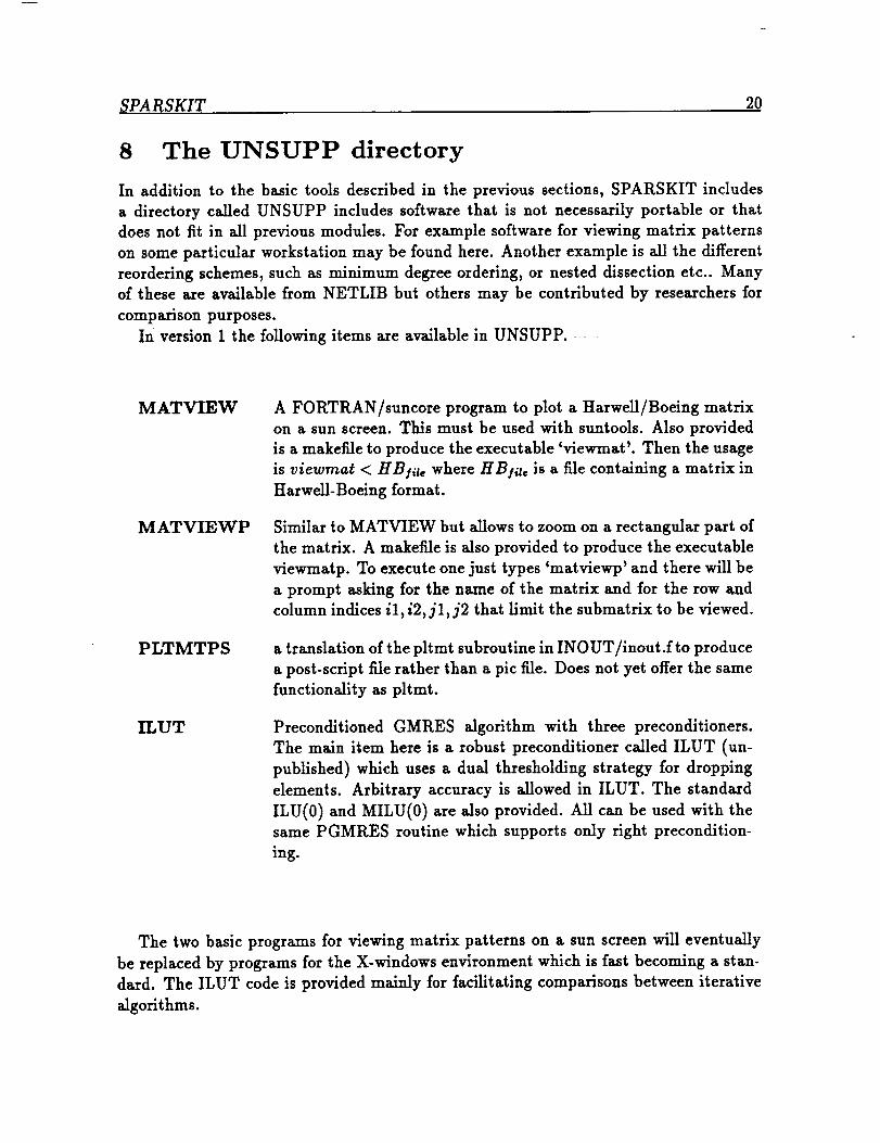
8 The UNSUPP directory
In addition to the basic tools described in the previous sections, SPARSKIT includes
a directory called UNSUPP includes software that is not necessarily portable or that
does not fit in all previous modules. For example software for viewing matrix patterns
on some particular workstation may be found here. Another example is all the different
reordering schemes, such as minimum degree ordering, or nested dissection etc.. Many
of these are available from NETLIB but others may be contributed by researchers for
comparison purposes.
In version 1 the following items are available in UNSUPP. _
MATVIEW
MATVIEWP
PLTMTPS
ILUT
A FORTRAN/suncore progrmm to plot a Harwell/Boeing matrix
on a sun screen. This must be used with suntools. Also provided
is a makefile to produce the executable 'viewmat'. Then the usage
is viewraat < HBII_ e where HBlil, is a file containing a matrix in
HarweU-Boeing format.
Similar to MATVIEW but allows to zoom on a rectangular part of
the matrix. A makefile is also provided to produce the executable
viewmatp. To execute one just types 'matviewp' and there will be
a prompt asking for the name of the matrix and for the row and
column indices il, i2,jl,j2 that limit the submatrix to be viewed.
a translation of the pltmt subroutine in INOUT/inout.f to produce
a post-script file rather than a pic file. Does not yet offer the same
functionality as pltmt.
Preconditioned GMRES algorithm with three preconditioners.
The main item here is a robust preconditioner called ILUT (un-
published) which uses a dual thresholding strategy for dropping
elements. Arbitrary accuracy is allowed in ILUT. The standard
ILU(0) and MILU(0) are also provided. All can be used with the
same PGMRES routine which supports only right precondition-
ing.
The two basic programs for viewing matrix patterns on a sun screen will eventually
be replaced by programs for the X-windows environment which is fast becoming a stan-
dard. The ILUT code is provided mainly for facilitating comparisons between iterative
algorithms.

SPARSKIT 21
9 Distribution
The first release of the package follows the Linpack-Eispack approach in that it aims at
providing ei_cient and well tested subroutines written in portable FORTRAN. Similarly
to the Linpack and Eispack packages, the goal is to make available a common base of
useful codes for a specific area of computation, in this case sparse linear algebra. The
package is in the public domain and will be made accessible through the internet.
Currently, the package is organized in six distinct subdirectorles, each containing one
or more modules. The six directories and the modules they contain are the following:
INOUT (inout.f), FORMATS (formats.f, unary.f), BLASSM (blassm.f, matvec.f), MAT-
GEN (genmat.f, zlatev.f), INFO (dinfol.f), UNSUPP (various routines). Test programs
with unix makefiles are provided in each subdirectory to test a large number of the sub-
routines. Each directory contains a README file listing contents, and giving additionalinformation.
For information concerning distribution contact the author at na.saad_na-net.stanford.edu.
10 Conclusion and Future Plans
It is hoped that SPARSKIT will be useful in many ways to researchers in different
areas of scientific computing. In the first version of SPARSKIT, there axe few sparse
problem solvers, such as direct solution methods, or eigenvalue solvers. Some of these
are available from different sources and we felt that it was not appropriate to provide
additional ones. The original motivation for SPARSKIT is that there is a gap to fill in
the manipulation and basic computations with sparse matrices. Once this gap is f_ed
with some satisfaction, then additional functionality may be added.
We briefly mentioned in the introduction the possibility of using SPARSKIT to de-
velop an interactive package. Large matrices of dimension tens of of thousands can easily
be manipulated with the current supercomputers, in real time. One of the dlil_culties
with such an interactive package is that we do not yet have reliable routines for com-
puting eigenvalues/eigenvectors of large sparse matrices. The state of the art in solving
linear systems is in a much better situation. However, one must not contemplate to
perform the same type of computations as with small dense matrices. As an example,
getting all the eigenvalues of a sparse matrix is not likely to be too useful when the
matrix is very large.
Beyond interactive software for sparse linear algebra, one can envision the integration
of SPARSKIT in a larger package devoted to solving certain types of Partial Differential
Equations, possibly interactively.
,_PARSKIT 22
Acknowledgements. The idea of creating a tool package for sparse matrices germi-
nated while the author was at the Center for Supercomputing Research and Development
of the University of Illinois (1986-1987) and part of this work was performed there. Ini-
tially the author has benefited from helpful comments from Iain Duff (then visiting
CSRD) and a number of colleagues at CSRD. Billy Stewart and his students at NCSU
used a preliminary version of SPARSKIT in a class project and made some valuable com-
ments. Ernie Rothman _ontributed some software. The author has also benefited from
helpful discussions from a number of other colleagues, including Mike Heroux, Giuseppe
Radicatti, Ahmed Sameh, Horst Simon, Phuong Vu, and Harry Wijshoff.
References
[1]
[2]
[3]
[4]
[51
[61
[7]
[8]
[9]
[lO]
E. C. Anderson and Y. Sand. Solving sparse triangular systems on parallel comput-
ers. Technical Report 794, University of Illinois, CSRD, Urbana, IL, 1988.
I. S. Duff. A survey of sparse matrix research. In Proceedings of the IEEE, 65,
pages 500-535, Prentice Hall, New York, 1977.
I. S. Duff, A. M. Erisman, and J. K. Reid. Direct Methods for Sparse Matrices.
Clarendon Press, Oxford, 1986.
I. S. Duff, R. G. Grimes, and J. G. Lewis. Sparse matrix test problems. ACM trans.
Math. Soft., 15:1-14, 1989.
T. C. Oppe Wayne Joubert and D. R. Kincaid. NSPCG User's guide. A Package
for Solving Large Linear Systems by Various Iterative Methods. Technical Report ,
The University of Texas at Austin, 1988.
T. C. Oppe and D. R. Kincaid. The performance of ITPACK on vector computers
for solving large sparse linear systems arising in sample oil reservoir simulation
problems. Communications in applied numerical methods, 2:1-7, 1986.
O. Osterby and Z. Zlatev. Direct methods for sparse matrices. Springer Verlag,
New York, 1983.
Y. Sand. Krylov subspace methods on supercomputers. SIAM J. Scient. Star.
Comput., 10:1200-1232, 1989.
D. M. Young, T.C. Oppe, D. R. Kincaid, and L. J. Hayes. On the use of vector com-
puters for solving large sparse linear systems. Technical Report CNA-199, Center
for Numerical Analysis, University of Texas at Austin, Austin, Texas, 1985.
Z. Zlatev, K. Schaumburg, and J. Wasniewskl. A testing scheme for subroutines
solving large linear problems. Computers and Chemistry, 5:91-100, 1981.

SPARSKIT 23
APPENDIX" QUICK REFERENCE
For convenience we list in this appendix the most important subroutines in the various
modules of SPARSKIT. More detailed information can be found either in the body of
the paper or in the documentation of the package.
FORMATS Module
• CSRDNS : converts a row-stored sparse matrix into the dense format.
• DNSCSR : converts a dense matrix to a sparse storage format.
• COOCSR : converts coordinate to to csr format
• COICSR : in-place conversion of coordinate to csr format
• CSRCO0 : converts compressed sparse row to coordinate format.
• CSRSSR : converts compressed sparse row to symmetric sparse row format.
• SSRCSR : converts symmetric sparse row to compressed sparse row format.
• CSRELL : converts compressed sparse row to ellpack format
• ELLCSR : converts ellpack format to compressed sparse row format.
• CSRMSR : converts compressed sparse row format to modified sparse row format.
• MSRCSR : converts modified sparse row format to compressed sparse row format.
• CSRCSC : converts compressed sparse row format to compressed sparse column
format (transposition).
• CSRDIA : converts the compressed sparse row format into the diagonal format.
• DIACSR : converts the diagonal format into the compressed sparse row format.
• BSRCSR : converts the block-row sparse format into the compressed sparse row
format.
• CSRBSR : converts the compressed sparse tow format into the block-row sparse
format.
• CSRBND : converts the compressed sparse row format into the banded format
(linpack style).
_qPARSKIT 24
• BNDCSR : converts the banded format (linpack style) into the compressed sparse
row storage.
• CSRSSK : converts the compressed sparse row format to the symmetric skyline
format
• SSKSSR : converts symmetric skyline format to symmetric sparse row format.
• CSRJAD : converts the csr format into the jagged diagonal format
• JADCSR : converts the jagged-diagonal format into the csr format
• COOELL : converts the coordinate format into the Ellpack/Itpack format.
UNARY Module
• SUBMAT : extracts a submatrix from a sparse matrix.
• FILTER : filters elements from a matrix according to their magnitude.
• TRANSP : in-place transposition routine (see also csrcsc in formats)
• COPMAT : copies a matrix into another matrix (both stored csr).
• GETDIA : extracts a specified diagonal from a matrix.
• GETL : extracts lower triangular part.
• GETU : extracts upper triangular part.
• LEVELS : gets the level scheduling structure for lower triangular matrices.
• AMASK : extracts C = A ® M
• DPERM : permutes a matrix (B = PAQ) given two permutations P, Q
• CPERM : permutes the columns of a matrix (B = AQ)
• RPERM : permutes the rows of a matrix (B = PA)
• VPERM : permutes a vector (in-place)
• RETMX : returns the max absolute value in each row of the matrix.
• DIAPOS : returns the positions of the diagonal elements in A.
• EXTBDG : extracts the main diagonal blocks of a matrix.
• GETBWD : returns the bandwidth information on a matrix.

SPARSKIT 25
• BLKFND : finds the block-size of a matrix.
• BLKCHK : checks whether a given integer is the block size of A.
• INFDIA : obtains information on the diagonals of A.
• AMUBDG : obtains the number of nonzeros in each row of AB.
• APBDGR : obtains the number of nonzero elements in each row of A q- B.
• RNRMS : computes the norms of the rows of A.
• CNRMS : computes the norms of the columns of A.
• RSCAL : scales the rows of a matrix by their norms.
• CSCAL : scales the columns of a matrix by their norms.
INOUT Module
• READMT : reads matrices in the boeing/HarweU format.
• PRTMT : prints matrices in the boeing/HarweU format.
• PLTMT : produces a 'pic' file for plotting a sparse matrix.
INFO Module
• DINFO1 : obtains a number of statistics on a sparse matrix.
MATGEN Module
• GEN57PT : generates 5-point and 7-point matrices.
• GEN5?BL : generates block 5-point and ?-point matrices.
• GENFEA : generates finite element matrices in assembled form.
• GENFEU : generates finite element matrices in unassembled form.
• ASSMB1 : assembles an unassembled matrix (as produced by genfeu).
• MATRF2 : Routines for generating sparse matrices by Zlatev et al.
• DCN: Routines for generating sparse matrices by Zlatev et al.

SPARSKIT 26
• ECN: Routines for generating sparse matrices by Zlatev et al.
BLASSM Module
• AMUB : computes C = A* B .
• BPLB : computes C = A -{- B .
• APLSB : computes C = A + sB.
• APMBT : Computes C = A + B r.
• APLSBT : Computes C = A + 8 * B T .
• DIAMUA : Computes C = Diag * A .
• AMUDIA : Computes C = A * Diag.
• APLDIA : Computes C = A +Diag.
• APLSCA : Computes A := A + sI (8 = scalar).
MATVEC Module
• AMUX : A times a vector. Compressed Sparse Row (CSR) format.
• ATMUX : A T times a vector. CSR format.
• AMUXE : A times a vector. Ellpack/Itpack (ELL) format.
• AMUXD : A times a vector. Diagonal (DIA) format.
• AMUXJ : A times a vector. Jagged Diagonal (JAD) format.
• LSOL : Unit lower triangular system solution. Compressed Sparse Row (CSR)
format.
• LDSOL : Lower triangular system solution. Modified Sparse Row (MSR) format.
• LSOL : Unit lower triangular system solution. Compressed Sparse Column (CSC)
format.
• LDSOLC: Lower triangular system solution. Modified Sparse Column (MSC) for-
mat.
• LDSOLL: Lower triangular system solution with level scheduling. MSR format.

SPA RSKIT 2 7
• USOL : Unit upper triangular system solution. Compressed Sparse Row (CSR)
format.
• UDSOL : Upper triangular system solution. Modified Sparse Row (MSR) format.
• USOLC : Unit upper triangular system solution. Compressed Sparse Column
(CSC) format.
• UDSOLC: Upper triangular system solution. Modified Sparse Column (MSC)
format.
UNSUPP Module
• ILUT: ILUT(k) preconditioned GMRES mini package.
• MATVIEW : suncore code for viewing a matrix on a sun station.
• MATVIEWP: suncore code for viewing a submatrix on a sun station.
• PLTMTPS : creates a post Script file to plot a sparse matrix.