Embed Size (px)
Citation preview
8/3/2019 V. N. Yershov- Equilibrium configurations of tripolar charges
http://slidepdf.com/reader/full/v-n-yershov-equilibrium-configurations-of-tripolar-charges 1/22
a r X i v : p h y s i c s / 0 6 0 9 1 8 5 v 1
[ p h y s i c s . g e n - p h ] 2 1 S e p 2 0 0 6
Equilibrium configurations of tripolar charges
V. N. Yershov
Mullard Space Science Laboratory
(University College London),Holmbury St.Mary, Dorking RH5 6NT, UK
Abstract
It is shown that an ensemble of particles with tripolar (colour) charges will necessarily cohere in ahierarchy of structures, from simple clusters and strings to complex aggregates and cyclic molecule-like structures. The basic combinatoric rule remains essentially the same on different levels of thehierarchy, thus leading to a pattern of resemblance between different levels. The number of primitivecharges in each structure is determined by the symmetry of the combined effective potential of this structure. The outlined scheme can serve as a framework for building a model of compositefundamental fermions. PACS: 89.75.Fb, 36.90.+f, 12.60.RC, 12.15.Ff.
1 Introduction
It is known that the structures of important objects that physicists study, like stars, galaxies, molecules,atoms, nucleons, and some particles, are equilibrium states between opposing forces of nature. Equilib-rium potentials are broadly used for modelling molecules [1, 2], vortices in superconductors [3, 4], metalstructures [5], and even granular materials [6]. Realistic interactions between molecules are known tohave always attractive and repulsive components, due to the fact that solids and liquids have the prop-erty of cohesion but, at the same time, do not collapse to a point under the action of these forces. Suchsystems are modelled with potentials that comprise a repulsive inner and an attractive outer region (orvice versa). A similar approach is often used in biochemistry [7], colloid chemistry [8], in material sciences[9], and many other branches of physics and chemistry.
In condensed matter, the interactions between neutral atoms are described by the equilibriumLennard-Jones and Morse potentials. The electron cloud of a neutral atom fluctuates about the pos-itively charged nucleus. The fluctuations in neighbouring atoms become correlated, inducing attractivedipole-dipole interactions. The equilibrium distance between two proximal atomic centres is determinedby a trade-off between this attractive (van der Waals) dispersion force and a core-repulsion force thatreflects electrostatic repulsion and the Pauli exclusion principle.
For simplicity, the Lennard-Jones forces are typically modelled as effectively pair-wise additive, andthe velocities and positions of atoms are calculated by numerical methods as a multi-body problemof mechanics. The effective potential in these systems is represented as a sum of one-body, two-bodyand three-body components. The task can be simplified by coupling two-body and higher multi-atomcorrelations in one model [10]. The central idea is that in real systems, the strength of each bond dependson the local environment, i.e. an atom with many neighbours forms weaker bonds than an atom withfew neighbours. Then, one can use a pair potential, the strength of which depends on the environment(screened potential in the Morse form). This is related to the exponential decay dependence of theelectronic density and is usually written as:
i
E i =1
2
i=j
V ij ,
V ij(rij ) = F C (rij )[F ⊖(rij ) + bijF ⊕(rij )],
(1)
where the potential energy is resolved into a site energy E i and a bonding energy V ij between the particlesi and j; rij is the distance between the particles (atoms); F ⊖ and F ⊕ are the attractive and repulsive
1
8/3/2019 V. N. Yershov- Equilibrium configurations of tripolar charges
http://slidepdf.com/reader/full/v-n-yershov-equilibrium-configurations-of-tripolar-charges 2/22
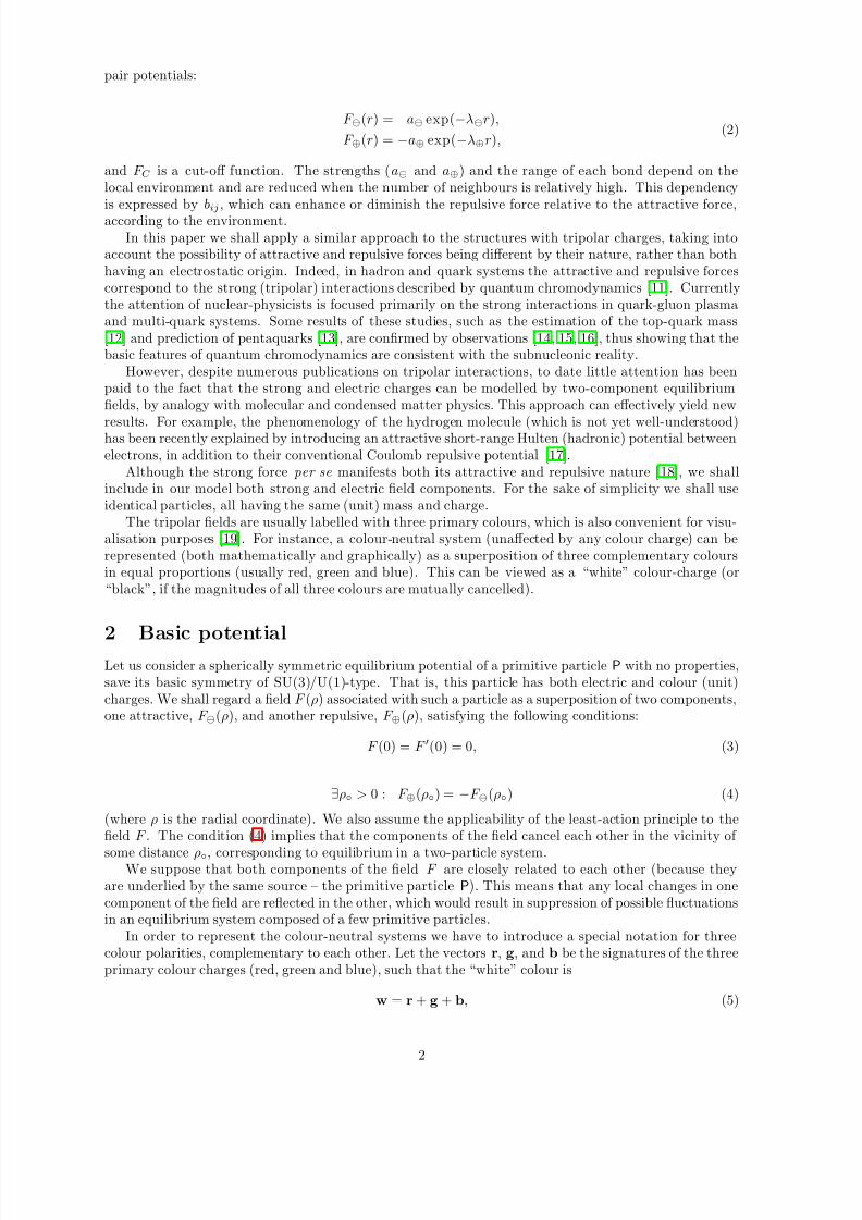
pair potentials:
F ⊖(r) = a⊖ exp(−λ⊖r),
F ⊕(r) = −a⊕ exp(−λ⊕r),(2)
and F C is a cut-off function. The strengths (a⊖ and a⊕) and the range of each bond depend on thelocal environment and are reduced when the number of neighbours is relatively high. This dependencyis expressed by bij , which can enhance or diminish the repulsive force relative to the attractive force,according to the environment.
In this paper we shall apply a similar approach to the structures with tripolar charges, taking intoaccount the possibility of attractive and repulsive forces being different by their nature, rather than bothhaving an electrostatic origin. Indeed, in hadron and quark systems the attractive and repulsive forcescorrespond to the strong (tripolar) interactions described by quantum chromodynamics [11]. Currentlythe attention of nuclear-physicists is focused primarily on the strong interactions in quark-gluon plasmaand multi-quark systems. Some results of these studies, such as the estimation of the top-quark mass[12] and prediction of pentaquarks [13], are confirmed by observations [14, 15, 16], thus showing that thebasic features of quantum chromodynamics are consistent with the subnucleonic reality.
However, despite numerous publications on tripolar interactions, to date little attention has beenpaid to the fact that the strong and electric charges can be modelled by two-component equilibriumfields, by analogy with molecular and condensed matter physics. This approach can effectively yield new
results. For example, the phenomenology of the hydrogen molecule (which is not yet well-understood)has been recently explained by introducing an attractive short-range Hulten (hadronic) potential betweenelectrons, in addition to their conventional Coulomb repulsive potential [17].
Although the strong force per se manifests both its attractive and repulsive nature [18], we shallinclude in our model both strong and electric field components. For the sake of simplicity we shall useidentical particles, all having the same (unit) mass and charge.
The tripolar fields are usually labelled with three primary colours, which is also convenient for visu-alisation purposes [19]. For instance, a colour-neutral system (unaffected by any colour charge) can berepresented (both mathematically and graphically) as a superposition of three complementary coloursin equal proportions (usually red, green and blue). This can be viewed as a “white” colour-charge (or“black”, if the magnitudes of all three colours are mutually cancelled).
2 Basic potentialLet us consider a spherically symmetric equilibrium potential of a primitive particle P with no properties,save its basic symmetry of SU(3)/U(1)-type. That is, this particle has both electric and colour (unit)charges. We shall regard a field F (ρ) associated with such a particle as a superposition of two components,one attractive, F ⊖(ρ), and another repulsive, F ⊕(ρ), satisfying the following conditions:
F (0) = F ′(0) = 0, (3)
∃ρ◦ > 0 : F ⊕(ρ◦) = −F ⊖(ρ◦) (4)
(where ρ is the radial coordinate). We also assume the applicability of the least-action principle to thefield F . The condition (4) implies that the components of the field cancel each other in the vicinity of
some distance ρ◦, corresponding to equilibrium in a two-particle system.We suppose that both components of the field F are closely related to each other (because they
are underlied by the same source – the primitive particle P). This means that any local changes in onecomponent of the field are reflected in the other, which would result in suppression of possible fluctuationsin an equilibrium system composed of a few primitive particles.
In order to represent the colour-neutral systems we have to introduce a special notation for threecolour polarities, complementary to each other. Let the vectors r, g, and b be the signatures of the threeprimary colour charges (red, green and blue), such that the “white” colour is
w = r + g + b, (5)
2
8/3/2019 V. N. Yershov- Equilibrium configurations of tripolar charges
http://slidepdf.com/reader/full/v-n-yershov-equilibrium-configurations-of-tripolar-charges 3/22
where w is the diagonal of a unit matrix. In order to satisfy (5), the rgb-vectors could have the followingcomponents:
r = (−1, +1, +1)⊺
g = (+1, −1, +1)⊺
b = (+1, +1, −1)⊺.
(6)
In the case of a system with mutually cancelled colour charges we can write
r + g + b−w = 0, (7)
which would correspond to a colour-neutral system with null electric charge.With this notation, the field F i(ρ) of a particle Pi that has a colour ci ∈ {r,g,b} can be written as
Fi(ρ) = ciF ⊕(ρ) + (ci −w/3)F ⊖(ρ). (8)
In particular, in a system with N = 3 complementary colour charges (say, c1 = r, c2 = g, c3 = b), thesuperposition of the fields F i will contain only the terms with F ⊕:
3i=1
Fi = wF ⊕,
because3
i=1
(ci −w/3) = 0,
and the terms with F ⊖ are mutually cancelled.As a simple example of the split equilibrium field one can consider the field with the following com-
ponentsF ⊖ = F 0(ρ), F ⊕ = F ′0(ρ), (9)
whereF 0(ρ) = sija0 exp(−λ0ρ−1). (10)
The derivative in (9) is taken with respect to the radial coordinate, ρ. The coefficient sij = ±1 (signature)
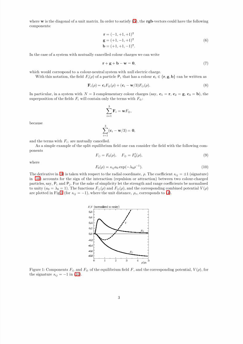
in (10) accounts for the sign of the interaction (repulsion or attraction) between two colour-chargedparticles, say, Pi and Pj . For the sake of simplicity let the strength and range coefficients be normalisedto unity (a0 = λ0 = 1). The functions F ⊖(ρ) and F ⊕(ρ), and the corresponding combined potential V (ρ)are plotted in Fig.1 (for sij = −1), where the unit distance, ρ◦, corresponds to (4).
ººº
ºº º
º º º º º º
º º º º º
ºº
ºº
º
º
º
º
º
º
º
º
º
º
º
º
º º
º
º
º º
º
º
º
º
º
º
º
º
º
º
º
º
º º º º
º º º
ºº
º
º
º
º
º
º
º
º
º
º
º
º
º
º
º
º
º
º
º
º
º
º
º
º
º
º
º
º
º
º
º
º
º º
º
º
º º
º º º
º º º
º º º
º
º
º
º
º
º
º
º
º
º
º
º
º
º
º
º
º
º
º
º
º
º
º
º
º
º
º
º
º
º
º
º
º
º
º
º
º
º
º
º
º
º
º
º
º
º
º
º
º
º
º
º
º
º
º
º
º
º
º
º
º
º
º
º
º
º
º
º
º
º
º
º
º
º
º
º
º
º
º
º
º
º
º
º
º
º
º
º
º
º
º
º
º
º
º
ºº
º
º
º
º
º
º
º
º
º
º
º
º
º
º
º
º
º
º
º
º
º
º
º
º
º
º
º
º
º
º
º
º
º
º
º
º
º
º
º
º
º
º
º
º º
ºº
º
º
º
º
º
º
ºº
º
º
º
º º
º
º
º
ºº
º
º
ºº
ºº
º
º
ºº
º
º
ºº
º
ºº
º
º
ºº
º
ºº
º
º
ºº
º º
º
ºº
º
ºº
ºº
º
ºº
º
ºº
ºº
º
ºº
º º
ºº
ºº
º
ºº
ºº
º
ººº
º
ºº
ººº
º
ºº
ºº º
º
ººº
º
ººº
ºº
ºº
ºº
ºº
ººº
ºº
ºº
ººº
º ºº
º
ººº
ºº
ººº
º º º º
º
º º º º
º
º º º º
ººº
ºº
º º º º
ºº º
ºº
º º º º
ºº
º º º º
º º º º
ºº
º º º º
ºº
º º º º º
º º º º
ºº
º º º º º
ºº ººº
ºº
º º º º º
ººº
º º º º º
º º º º º
ºº
º º º º º º
ºº
º º º º º º
ºº
º º º º º
ºº
º º º º
º
º
º
º
º
º
º
º
º
º
º
º
º
º
º
ºº
º º
º
º º
º
º º
º
º
º
º
º
º
º º
º
º
º
º
º
º
º
º
º
º
º
º
º
º
º
º
º
º
º
º
º
º
º
º
º
º
º
º
º
º
º
º
º
º
º
º
º
º
º
º
º
º
º
º
º
º
º
º
º
º
º
º
º
º
º
º
º
º
º
º
º
º
º
º
º
º
º
º
º
º
º
º
º
º
º
º
º
º º
ºº
º
º º º
º º
º
º º º º º
º º º
º º º º º º º º º º
º º º
º º º º º
º
º º
º º
º
º º
º º
º
º º
º
º
º
º
º
º
º
º
º º
º
º º
º
º
º
º
º
º
º
º
º
º
º
º
º
º
º
º
º
º
º
º
º
º
º
º
º
º
º
º
º
º
º
º
º
º
º
º
º
º
º
º
º
º
º
º
º
º
º
º
º
º
º
º
º
º
º
º
º
º
º
º
º
º
º
º
º
º
ºº
º º
º
ºº º
º
º
º
ºº
º
º
º
º
º
º
º
º
º
º
ºº
º
º
º
º
º
º
º º
º
º
º
º
º
º
º
º
º
º
º
º
º
º
º
º
º
º
º
º
º
º
º
º
º
º
º
º
º
º
º
º
º
º
º
º
º
º
º
º
º
º
º
º
º
º
º
º
º
º
º
º
º
º
º
º
º
º
º
º
º
º
º
º
º
º
º
º
º
º
º
º
º
º
º
º
º
º
º
º
º
º
º
º
º
º
º
º
º
º
º
º
º
º
º
º
º
º
º
º
º
º
º
º
ºº
ºº
ºº
º
º
ºº
º
º
ºº
º
º
ºº
º
ºº
º º
º
º
º
ºº
º ºº
º
ºº
º
ºº
ºº
º
ººº
º º
ºº
ºº
º
ººº
ºº º
º
ººº
ºº
ººº
ººº
ºº
ººº
ºº ºº
º
º º º º
ºº
º º º º
ºº ºº
ºº
º º º º º
ºº
º º º º º
º º º º º
ºº
º º º º º º
ºº ºº º
ººº
º º º º º º
º º º º
º º º º º º
º º º º ººº
º º º º
º º º º º º º º
º º º º
º º º º º º º º º
º º º º º º º º º
º º º º º
º º º º º º º º º º º
º º º º º º º º º º º
º º º º º º
º º º º º º º º º º º º ºº
º º º º º º º
º º º º º º º º º º º º ºº
ººº
ºº º
ºº
ºº
ºº ºº
º
º
ºº
º
º
ºº º
º
º
º
º
º
º
º
º
º
º
º
º
º
º
º
º º
º
º º
º º º º º º
º º
º
º
º
º
º
º
º
º
º
º
º
º
º
º
º º
º
º
º
º
ºº
º º
º
º ººº
º º º º
º
ººº
ºº º
º
º
ºº
ºº
º
º
º
º
º
º
º º
º
º
º
º
º
º
º
º
º
º
º
º
º
º
º
º
º
º
º º
º
º
º
º
º º
º
º
º
º
º
º
º
º
º
º
º
º
º
º
º
º
º
º
º
º
º
º
º
º
º
º
º
º
º
º
º
º
º
º
º
º
º
º
º
º
º º
º
º
º
º
º
º
º
º º
º
º
º
º
º
º
º
º º
º
º
º
º
º
º
º
º
º º
º
º
º
º
º
º
º
º
º º
º
º
º
º
º
º
º
º
º º
º
º
º
º
º
º
º
º
º º
º
º
º
º
º
º
º
º
º º
º
º
º
º
º
º
º
º
º
º º
º
º
º
º
º
º
º
º
º º
º
º
º
º
º
º
º
º
º
º
º
º
º
º
º
º
º
º
º
¼ ½ ¾ ¿
¼
¼
¼
¼
¼ ¾
¼ ¼
¹ ¼ º ¾
¹ ¼ º
¹ ¼ º
¹ ¼ º
©
Î
Î ´ Ò Ó Ö Ñ Ð × Ø Ó Ù Ò Ø Ý µ
Figure 1: Components F ⊖ and F ⊕ of the equilibrium field F , and the corresponding potential, V (ρ), forthe signature sij = −1 in (10).
3
8/3/2019 V. N. Yershov- Equilibrium configurations of tripolar charges
http://slidepdf.com/reader/full/v-n-yershov-equilibrium-configurations-of-tripolar-charges 4/22
3 Colour dipoles and tripoles
Obviously, the simplest structures allowed by the tripolar field are the monopoles, dipoles and tripoles,unlike the conventional bipolar (electric) field, which allows only the monopoles and dipoles. Here weshall consider the colour dipoles and tripoles. The potentials shown in Fig.1 correspond to a pair of like-charged (F ⊕ – repulsive) primitive particles with unlike-colours (F ⊖ – attractive), which constitutea charged colour dipole C2ij = Pi + Pj . Here the indices i and j label the colour charges of the dipole’sconstituents: i, j ∈ {r,g,b}, i = j; the upper index “2” stands for the number of particles involved. As
with any other dipole, the components of C2
ij will oscillate near an equilibrium point at ρ = ρ◦, wherethe potential V (ρ) has a minimum. The two components of F are approximately antisymmetric in thevicinity of the origin, which would lead to suppression of these oscillations. Then, the estimation of theground-state energies (masses) of such a system will be simplified because one can neglect the oscillatoryenergy of Pi and Pj and, to a first-order approximation, compute the mass of the system as a sum of themasses of its constituents.
The existence of a second stationary point in the potential – at the origin – means that the dipole’sconstituents, if confined within a very small volume, can be found in a spherically-symmetric superpositionstate at ρ = 0. But this state is unstable and its spherical symmetry can be spontaneously broken, withρ → ρ◦, resulting in the polarisation of the system. This also breaks another fundamental symmetry –that of scale invariance.
Given the field F (ρ) being split in two components, the rest energy of the particle P,
−∞ 0
F (ρ)dρ,
can be resolved into two parts, containing
∞ 0
F ⊖(ρ)dρ and
∞ 0
F ⊕(ρ)dρ, (11)
which can be viewed as two mass terms, mP and mP, respectively. With (10) normalised to unity, thesecond term, mP, is also a unity (let us denote this unit mass as m◦). But the first integral in (11) diverges(mP = ∞), implying that within the chosen approach the primitive colour charges cannot exist in freestates because of their infinite energies. The same is valid for the case of the colour-dipole, C2ij, which has
(a) (b)
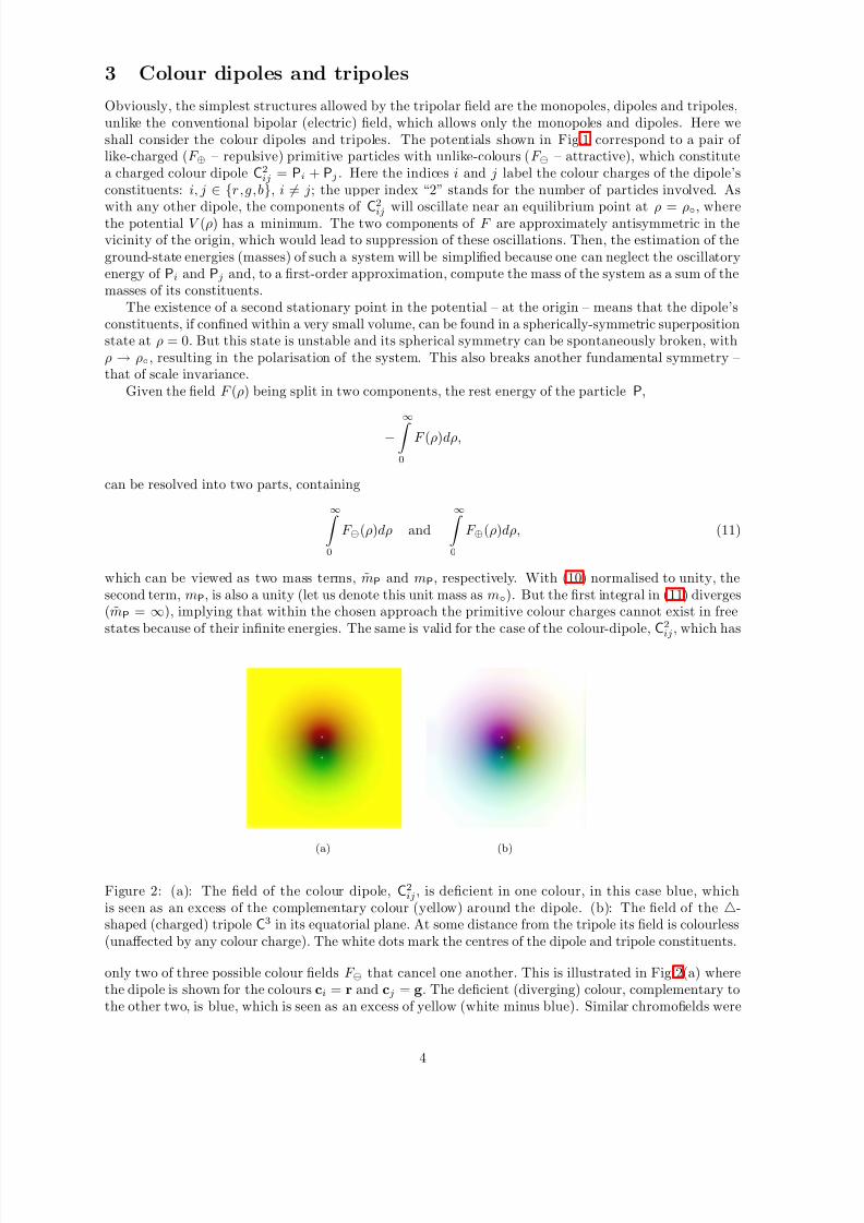
Figure 2: (a): The field of the colour dipole, C2ij , is deficient in one colour, in this case blue, whichis seen as an excess of the complementary colour (yellow) around the dipole. (b): The field of the △-shaped (charged) tripole C3 in its equatorial plane. At some distance from the tripole its field is colourless(unaffected by any colour charge). The white dots mark the centres of the dipole and tripole constituents.
only two of three possible colour fields F ⊖ that cancel one another. This is illustrated in Fig.2(a) wherethe dipole is shown for the colours ci = r and cj = g. The deficient (diverging) colour, complementary tothe other two, is blue, which is seen as an excess of yellow (white minus blue). Similar chromofields were
4
8/3/2019 V. N. Yershov- Equilibrium configurations of tripolar charges
http://slidepdf.com/reader/full/v-n-yershov-equilibrium-configurations-of-tripolar-charges 5/22
discussed in [20], based on the Gaussian dielectric function and chiral chromodielectric model [21, 22],and also in [23].
Returning to the particle (inertial) masses, we must note that in the current literature there is noagreement as to the origin of mass or inertia. In the Standard Model of particle physics, the initiallymassless fundamental particles acquire their masses through interactions with the Higgs field. This iscurrently not yet supported by observations, and in this paper we are free to adhere to a different viewthat mass is a purely electromagnetic phenomenon. In the simplified approach of this paper we shallnot be considering any other forces rather than the electrostatic force caused by the equilibrium field
F (ρ). However, contrary to the conventional Coulomb gauge, we shall not regard the field F (ρ) as actinginstantaneously at a distance because this would be incompatible with the causality principle. It is moresensible to suggest that the field flow rate is not infinite. Then, there will be a time delay between theaction on one part of a system and the response from its another part. This can be viewed as inertia of the system, and the mass of such a system can be regarded as a measure of this delayed response to theexternal action. That is, the more components of the system are to respond to this action and the moremutually interacting components contribute to that response, the higher mass should be assigned to thissystem.
To formalise the calculation of masses, we shall represent the discharge of the primitive colour particlewith the use of auxiliary 3 × 3 singular matrices P
±
i containing the following elements:
± pijk = ±δi
j (−1)δkj , (12)
where δi
j is the Kronecker delta-function; the ±-signs correspond to the sign of the charge; and the indexi stands for the colour (i = 1, 2, 3 or red, green and blue). The diverging components of the field can berepresented by reciprocal elements:
˜ pjk = p−1jk .
Then, we can define the charges and masses of the primitive particles by summation of these matrixelements:
qP = w⊺Pw , qP = w⊺
Pw (13)
andmP = |w⊺
Pw| , mP = |w⊺Pw| (14)
(qP and mP diverge). The same matrices P can be used when calculating the signature sij in (10) forthe colours i and j:
sij =
−w⊺
PiPjw. (15)
In this notation the positively charged dipole C+ 2 (Fig.2a) can be represented as a sum of two matrices,
P+
1 and P+
2:
C+ 2= P
+
1 +P+
2 =
−1 +1 +1
+1 −1 +10 0 0
, (16)
with qC2 = +2 [q◦]. If two components of the dipole are oppositely charged:
C◦ 2= P
+
1 +P−
2 (17)
(of whatever colour combination), then their electric fields cancel each other:
qC◦ 2 = 0 (18)
implying also a negligibly small mass of this neutral dipole. Of course, the complete cancellation of thefields is possible only if the centres of both charges coincide; otherwise, the system is polarised (as withany dipole). The degree of polarisation would depend on the distance between the components. Let usdefine the mass of a system containing, say, N particles, as proportional to the number of these particles,wherever their field flow rates are not cancelled. For this purpose, we shall consider (to a first-orderapproximation) the total field flow rate, vN , of such a system as a superposition of the individual volumeflow rates of its N components. Then, the total mass can be calculated as the number of particles, N ,times the normalised to unity field flow rate vN :
mN = |N vN |. (19)
5
8/3/2019 V. N. Yershov- Equilibrium configurations of tripolar charges
http://slidepdf.com/reader/full/v-n-yershov-equilibrium-configurations-of-tripolar-charges 6/22
Here vN is computed recursively as a (Lorentz additive) superposition of the individual flow rates, vi:
vi =qi + vi−1
1 + |qivi−1| , (20)
where i = 2, . . . , N ; and v1 = q1. The normalisation condition (20) expresses the common fact that thesuperposition flow rate of, say, two antiparallel flows (↑↓) with equal rate magnitudes |v↑| = |v↓| = vvanishes (v↑↓ = 0), whereas, in the case of parallel flows (↑↑) it cannot exceed the magnitudes of theindividual flow rates (v↑↑
≤v). With this notation, the mass of, for instance, the charged colour dipole
will be:m
C+ 2 ≈ 2, m
C+ 2 = ∞. (21)
The neutral colour dipole will be massless:
mC◦ 2 ≈ 0 (22)
but stillm
C◦ 2 = ∞ (23)
due to the null-elements in the matrix C◦ 2 (the dipole lacks, at least, one colour charge to make it colour-
neutral). The infinities in (21) and (23) imply that neither C+ 2 nor C
◦ 2 can exist in free states. Of course, the flow rate of the electric field of the neutral dipole (and its corresponding mass) is cancelledonly approximately (as with any dipole) because the centres of its constituents do not coincide. In an
ensemble of a large number of neutral dipoles C◦ 2, not only electric but all the chromatic components of
the field can be cancelled (statistically).Obviously, three complementary colour charges will tend to cohere and form a △-shaped structure
with the distance ρ◦ (of equilibrium) between its components. Thus, by completing the set of colour-
charges in the charged dipole (adding, for example, the blue-charged component to the system C+ 2 shown
in Fig.2a) one would obtain a colour-neutral (but electrically charged) △-shaped tripole:
C3 := [ g
r b] =△ . (24)
Hereafter, we shall use the above triangular notation in the structural diagrams representing differenttripole combinations (one must not mistake these diagrams for algebraic equations). The marked vertexof the triangle in (24) indicates one of the colour-charges, say, red, to visualise (in the structural diagrams)
possible rotations of tripoles with respect to each other. The positively charged △-shaped tripole (C
+ 3
or△+ ), which can be written in the matrix notation as
C+ 3= P
+
1 +P+
2 +P+
3 =
−1 +1 +1
+1 −1 +1+1 +1 −1
,
is colour-neutral at infinity but colour-polarised in the vicinity of its constituents (see Fig.2b). Both mand m of C3 are finite:
m△ = m△ = 3 [m◦],
since all of the diverging components in its combined chromofield are mutually cancelled (converted intothe binding energy of the tripole).
4 Two-component systems of tripoles
A part of the field of the tripole (in its equatorial plane) is ring-closed [24], whereas another part isextended (over the ring’s poles). In its equatorial plane, the tripole possesses 2π m
n -rotational symmetry(m ≤ n − 1, n = 2, 3) of the second- and third-order cyclic groups. With the dispersion of colour-charges,corresponding to this symmetry, different △-tripoles can combine into chains.
A pair of tripoles would combine pole-to-pole with each other forming a doublet (d). One can estimatethe potential energy of this system by computing the pair-wise forces between its constituents. The schemefor this computation is shown in Fig.3(a). The potential energy of the doublet depends on the positions of
6
8/3/2019 V. N. Yershov- Equilibrium configurations of tripolar charges
http://slidepdf.com/reader/full/v-n-yershov-equilibrium-configurations-of-tripolar-charges 7/22
º
º
º
º
º
º
º
º
º
º
º
º
º
º
º
º
º
º
º
º
º
º
º
º
º
º
º
º
º
º
º
º
º
º
º
º
º
º
º
º
º
º
º
º
º º
º
º
º º º
º º
º º º º
º º
º
º º
º
º
º
º
º
º
º
º
º
º
º
º
º
º
º
º
º
º
º
º
º
º
º
º
º
º
º
º
º
º
º
º
º
º
º
º
º
º
º
º
ºº
º º º º º º º º
º
ºº
º
º
º
º
º
º
º
º
º
º
º
º
º
º
º
º
º
º
º
º
º
º
ºº
ºº
º
º
ºº
ºº
º
º º
ºº
ºº
ºº
º
ºº
ºº
ºº
º
ºº
ºº
ºº
º
ºº
ºº
ºº
º
ºº
ºº
ºº
º
ºº
ºº
ºº
º
ºº
ºº
º
º
º
º
º
º
º
º
º
º
º
º
º
º
º
º º
º º º º º
º º
º
º
º
º
º
º
º
º
º
º
º
º
º
º
º
º
º
º
º
º
º
º
º
º
º
º
º
º
º
º
º
ºº
º º º º º
ºº
º
º
º
º
º
º
º
º
º
º
º
º
º
º
º
º
º
º
º
º
º
º
º
º
º
º
º
º
º
º
º
º
º
º
º
º
º
º
º
º
º
º
º
º
º
º
º
º
º
º
º
º
º
º
º
º
º
º
º
º
º
º
º
º
º
º
º
º
º
º
º
º
º
º
º
º
º
º
º
º º
º º
º º º
º
º
º
º
º
º
º
º
º
º
º
º
º
º
º
º
º
º
º
º
º
º
º
º
º
º
º
º
º
º
º
º
º
ºº
ºº
ººº
º
º
º
º
º
º
º
º
º
º
º
º
º
º
º
º
º
º
º
º
º
º
º
º
º
º
º
º
º
º
º
º
º
º
º
º
º
º
º
º
º
º
º
º
º
º
º
º
º
º
º
º
º
º
º
º
º
º
º
º
º
º
º
º
º
º
º º
º º
º
º º º º
º º
º º
º º
º
º
º
º
º
º
º
º
º
º
º
º
º
º
º
º
º
º
º
º
º
º
º
º
º
º
º
º
º
º
º
º
º
º
º
º
º
º
º
º
º
º
º
ºº
º º º º º º º
ºº
º
º
º
º
º
º
º
º
º
º
º
º
º
º
º
º
º
º
º
º
º
º
º
º
º
º
º
º
º
º
º
º
º
º
º
º
º
º
º
º
º
º
º
º
º
º
º
º
º
º
º
º
º
º
º
º
º
º
º
º
º
º
º
º
º
º
º
º
º
º
º
º
º
º
º
º
º
º
º
º
º
º
º
º
º
º
º
º
º
º
º
º
º
º
º
º
º
º º
º º º
º º
º
º
º
º
º
º
º
º
º
º
º
º
º
º
º
º
º
º
º
º
º
º
º
º
ºº
º
ººº
º
ºº
º
º
º
º
º
º
º
º
º
º
º
º
º º º
º º º º º
º º º º º
º º
º º º º º º
º º º º º
º º º º º
º º º º º
º º º
º º º º º
º º º º º
º º º º º
º º º
º º º º º
º
º
º
º
º
º
º
º
º
º
º
º
º
º
º
º º
º º º º º
º º
º
º
º
º
º
º
º
º
º
º
º
º
º
º
º
º
º
º
º
º
º
º
º
º
º
º
º
º
º
º
ºº
º
º º º º º
ºº
º
º
º
º
º
º
º
º
º
º
º
º
º
º
º
º
º º º º º
º º º º
º º º º
º º º º º
º º º º
º º º º
º º º º º
º º º º
º º º º
º º º º º º º
º º º º º º º º º º º º º º º º º º º º º ºº º
º º º º º º
º º º º º
º º º º
º º º º
º º º º º º º º º º º º
º
º
ºº
º º
º
º
ºº
ºº
º
ºº
ººº
ºº
º º º º
º
º
º º º º º º º º º º º º º º º º º º
º º º º
º º º º
º ººº
ºº
ºº
ººº
ºº
ºº
ºº
ºº
ºº
ºº
º
º
ººº
º
º
ºº
ºº
º
º
º
º
º
º º
º
º
º
ºº
º
º
º
º
º
ºº
º
º
º
º
º
º
º
ºº
º
º
º
º
º
º
º
º
º
º
º
º
º
º
º
º
º
º
º
º
º
º
º
º
º
º
º
º
º
º
º
º
º
º
º
º
º
º
º
º
º
º
º
º
º
º
º
º
º
º
º
º
º
º
º
º
º
º
º
º
º
º
º
º
º
º
º
º
º
º
º
º
º
º
º
º
º
º
º
º
º
º
º
º
º
º
º
º
º
º
º
º
º
º
º
º
º
º
º
º
º
º
º
º
º
º
º
º
º
º
º
º
º
º
º
º º
º
º
º
º
º
º
º
º
º
º
º
º
º
º
º
º
º
º
º
º
º
º
º
º
º
º
º
º
º
º
º
º
º
º
º º
º
º
º
º
ºº
º
º
º
º
º
º
º
º
º º
º
º
º
º
º
º
º
º
º
º
º
º
º
º
º
º ºº
º
º
º
ºº
º
º
ºº
º
ºº
ºº º
ººº
ºº
ººº
ºº
º ºº
º
ºº
º º º º º º º
º º º º
ºº
ººº
º
º
º
ºº
º
º
º
º
º
º
º
º
º
º
º
º
º
º
º
º
º
º
º
º
º
º
º
º
º
º
º
º
º
º
º
º
º
º
º
º
º
º
º
º
º
º
º
º
º
º
º
º
º
º
º
º
º
º
º
º
º
º
º
º
º
º
º
º
º
º
º
º
º
º
º
º
º
º
º
º
º
º
º
º
º
º
º
º
º
º
º
º
º
º
º
º
º
º
º
º
º
º
º
º
º
º
º
º
º
º
º
º
º
º
º
º º
º
º
º
º
º
º
º
º
º
º
º
º
º
º
º
º
º
º
º
º
º
º
º
º
º º
º
º
º
º
º
º
º
º
ºº
º
º
º
º
º
º
º
º
º
º
ºº
º
º
º
º
º
ºº
º
ºº
ºº
º º
º
ºº
º
ºº
ºº
º
º
º
º
º
º
º
º
º
º
º
º
º
º
º
º
º
º
º
º
º
º
º
º
º
º
º
º
º
º
º
º
º
º
º
º
º
º
º
º
º
º
º
º
ºº
ºº
º
º
º
º
ºº
ºº
º
º
º
º
ºº
ºº
ºº
º
ºº
ºº
º º
º
ººº
º º
º º º º
ººº
ººº
º º º º
º
º º
ººº
º
º
ººº
º
º
º
º º º º º º º
ººº
ººº
ººº
ººº
ººº
ºº
º
ºº
º º
ºº
ºº
º
ººº
º
º
º
ºº
º
º
º
º º
º
º
º
º
ºº
ºº
º
º
º
º
º
º
º
º
º
º
º
ºº
º
º
º
º
º
º
º
º
º
º
º
º
º
º
º
º
º
º
º
º
º
º
º
º
º
º
º
º
º
º
º
º
º
º
º
º
º
º
º
º
º
º
º
º
º
º
º
º
º
º
º
º
º
º
º
º
º
º
º
º
º
º
º
º
º
º
º
º
º
º
º
º
º
º
º
º
º
º
º
º
º
º
º
º
º
º
º
º
º
º
º
º
º
º
º
º
º
º
º
º
º º
º º
º
º º
º
º º
º º
º
º º
º º
º º
º º º
º
º º º º º º º º º º º º º º º º º
º
º º
º º
º
º º
º º
º º
º º
º
º
º º
º
º
º
º
º
º
º
º
º
º
º
º
º
º
º
º
º
º
º
º
º
º
º
º
º
º
º
º
º
º
º
º
º
º
º
º
º
º
º
º
º
º
º
º
º
º
º
º
º
º
º
º
º
º
º
º
º
º
º
º
º
º
º
º
º
º
º
º
º
º
º
º
º
ª
ª
ª
ª
º º º º ºº º º ºº º º º º ºº º º º º º º º º º º º ºº º º º º ºº º º º ºº º º º º ºº º º º º º º º º º º º ºº º º º º ºº º º ºº º º º º ºº º º
º º º º
º º º º
º º º º
º º º º º º º º º º º
º º º º º º º º º º º º
º º º º º º º º º º º
º º º º º
º º º º
º º º º
º º º º º
º º º º º
º º º
Ö
º º º º º
º º º º º º º
º º º º º º º
º º º º º º º
º º º º º º º
º º º º º º º
º º º º º º º
º º º º
º º º º º º º
º º º º º º º
º º º º º º º
º º º º º º º
º
º
º
º
º
º
º
º
º
º
º
º
º
º
º
º
º
º
º
º
º
º
º
º
º
º
º
º
º
º
º
º
º
º
º
º
º
º
º
º
º
º
º
º
º
º
º
º
º
º
º
º
º
º
º
º
º
º
º
º
º
º
º
º
º
º
º
º
º
º
º
º
º
º
º
º
º
º
º
º
º
º
º
º
º
º
º
º
º
º
º
º
º
º
º
º
º
º
º
º
º
º
º
º
º
º
º
º
º
º
º
º
º
º
º
º
º
º
º
º
º
º
º
º
º
º
º
º
º
º
º
º
º
º
º
º
º
º
º
º
º
º
º
º
º
º
º
º
º
º
º
º
º
º
º
º
º
º
º
º
º
º
º
º
º
º
º
º
º
º
º
º
º
Ö
Ö
Ö
º º º
º º
º
º
º
º º
º
º
º
º
º
º º º º º º º º º º º º º º º º º º º º
º º º º
º º
º º º
º º
º º º
º
º º
º º º
º
º
º
º º
º
º
º
º º
º
º º
º
º
º
º º
º
º
Ö
Á Â
· ¿
Á
· ¿
Â
Á
Â
Ü
Á
Ý
Á
Þ
Á
Ü
Â
Ý
Â
Þ
Â
ρIJρ◦
◦
ζ (a) (b)
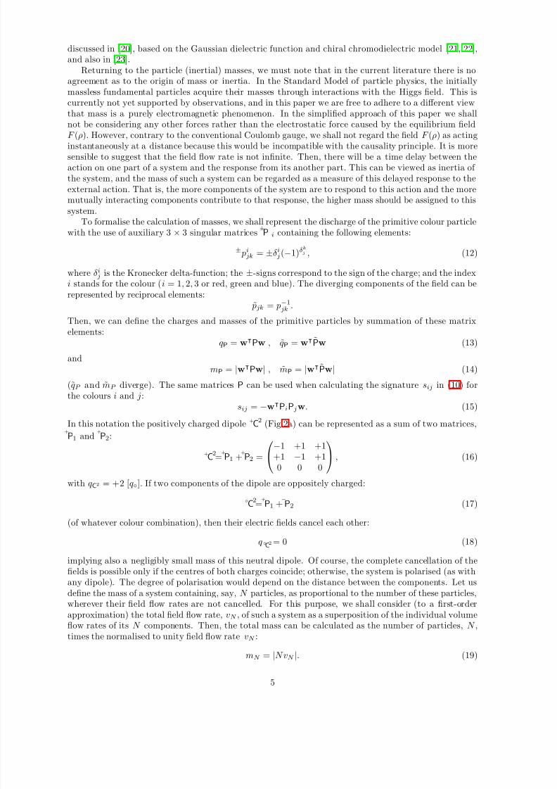
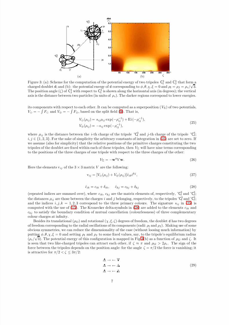
Figure 3: (a): Scheme for the computation of the potential energy of two tripoles C3I and C3J that form a
charged doublet d; and (b): the potential energy of d corresponding to φ,θ,χ,ξ = 0 and ρI = ρJ = ρ◦/√
3.The position angle (ζ ) of C3J with respect to C3I is shown along the horizontal axis (in degrees); the verticalaxis is the distance between two particles (in units of ρ◦). The darker regions correspond to lower energies.
its components with respect to each other. It can be computed as a superposition (V Σ) of two potentials,V ⊖ =
− F ⊖ and V ⊕ =− F ⊕, based on the split field (9). That is,
V ⊖(ρij ) = sijρij exp(−ρ−1ij ) + Ei (−ρ−1ij ),
V ⊕(ρij ) = −sij exp(−ρ−1ij ),(25)
where ρij is the distance between the i-th charge of the tripole C+ 3
I and j-th charge of the tripole C+ 3
J;i, j ∈ {1, 2, 3}. For the sake of simplicity the arbitrary constants of integration in (25) are set to zero. If we assume (also for simplicity) that the relative positions of the primitive charges constituting the twotripoles of the doublet are fixed within each of these tripoles, then V Σ will have nine terms correspondingto the positions of the three charges of one tripole with respect to the three charges of the other:
V Σ = −w⊺V w. (26)
Here the elements vij of the 3
×3 matrix V are the following:
vij = [V ⊖(ρij ) + V ⊕(ρij )]cikckj , (27)
cik = cik + δik, ckj = ckj + δkj (28)
(repeated indices are summed over), where cik, ckj are the matrix elements of, respectively, C+ 3
I and C+ 3
J;
the distances ρij are those between the charges i and j belonging, respectively, to the tripoles C+ 3
I and C+ 3
J;and the indices i,j,k = 1, 2, 3 correspond to the three primary colours. The signature sij in (25) iscomputed with the use of (15). The Kronecker delta-symbols in (28) are added to the elements cik andckj to satisfy the boundary condition of mutual cancellation (colourlessness) of three complementarycolour charges at infinity.
Besides its translational (ρIJ) and rotational (χ, ξ, ζ ) degrees of freedom, the doublet d has two degreesof freedom corresponding to the radial oscillations of its components (radii ρI and ρJ). Making use of someobvious symmetries, we can reduce the dimensionality of the case (without loosing much information) byputting φ,θ,χ,ξ = 0 and setting ρI and ρJ to some fixed values, say, to the tripole’s equilibrium radius(ρ◦/
√3). The potential energy of this configuration is mapped in Fig.3(b) as a function of ρIJ and ζ . It
is seen that two like-charged tripoles can attract each other, if ζ ≈ π and ρIJ > 2ρ◦. The sign of theforce between the tripoles depends on the position angle: for the angle ζ = π/2 the force is vanishing; itis attractive for π/2 < ζ ≤ 3π/2:
△+ → ← △ +
△+ → ← △+△+ → ← △+
(29)
7
8/3/2019 V. N. Yershov- Equilibrium configurations of tripolar charges
http://slidepdf.com/reader/full/v-n-yershov-equilibrium-configurations-of-tripolar-charges 8/22
and repulsive for |ζ | < π/2:
← △+ △+ →← △+ △ + →← △+ △ + → .
(30)
Thus, separated by distance ρIJ > 2ρ◦ two tripoles can combine into the configuration
d+ =
△+
△ + (or d
− =△−
△ −
). (31)
The existence of bifurcation points in the potential at ρIJ ≈ 2ρ◦ suggests the possibility of moving thesystem into a deeper potential well at ρ ≈ 0 by squeezing it below ρIJ = ρ◦ (and keeping ζ = 0).
The width of the central potential well (ζ = π, ρIJ > 2ρ◦) allows a certain degree of freedom for theconstituents of d to oscillate (rotating) within 2
3π < ζ < 4
3π:
d+↾ =△+ △+ ⇄ d
+⇂ =△+
△+ . (32)
The strength and sign of the force between the components depends on ζ . This implies the distance ρIJbeing covariant with ζ ; that is, the translational and rotational oscillations of the doublet are synchronous.Note that in (31) and (32) we put the symbols △+ side-by-side, implying, however, that they rotatecoaxially with respect to each other (θ, ξ = 0). The symbols ↾ and ⇂ in (32) denote the clockwise andanticlockwise rotations. Over again, we would like to stress that the diagrams (29)-(32) express not
otherwise than structural relationships (like, for instance, the formulae in organic chemistry), and by nomeans should they be mistaken for algebraic expressions.
ρIJρ◦
◦
ζ
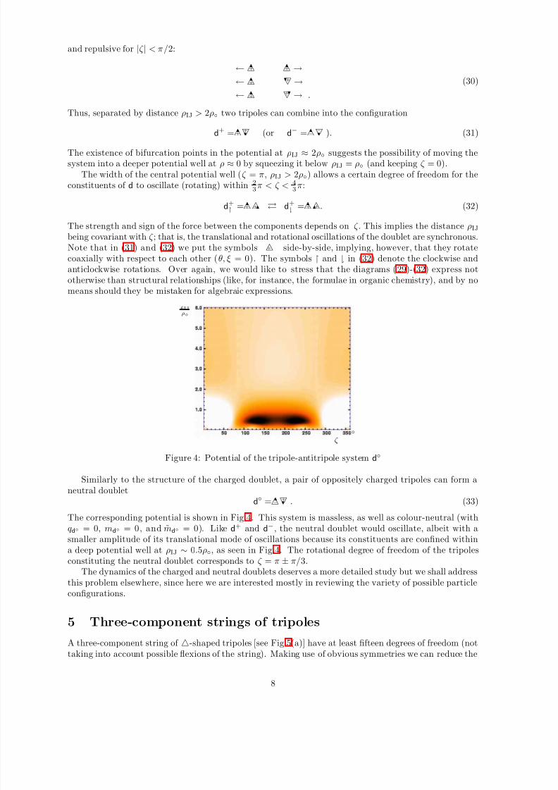
Figure 4: Potential of the tripole-antitripole system d◦
Similarly to the structure of the charged doublet, a pair of oppositely charged tripoles can form aneutral doublet
d◦ =△− △ +
. (33)
The corresponding potential is shown in Fig.4. This system is massless, as well as colour-neutral (withqd◦ = 0, md◦ = 0, and md◦ = 0). Like d+ and d−, the neutral doublet would oscillate, albeit with asmaller amplitude of its translational mode of oscillations because its constituents are confined within
a deep potential well at ρIJ ∼ 0.5ρ◦, as seen in Fig.4. The rotational degree of freedom of the tripolesconstituting the neutral doublet corresponds to ζ = π ± π/3.The dynamics of the charged and neutral doublets deserves a more detailed study but we shall address
this problem elsewhere, since here we are interested mostly in reviewing the variety of possible particleconfigurations.
5 Three-component strings of tripoles
A three-component string of △-shaped tripoles [see Fig.5(a)] have at least fifteen degrees of freedom (nottaking into account possible flexions of the string). Making use of obvious symmetries we can reduce the
8
8/3/2019 V. N. Yershov- Equilibrium configurations of tripolar charges
http://slidepdf.com/reader/full/v-n-yershov-equilibrium-configurations-of-tripolar-charges 9/22
º
º
º
º
º
º
º
º
º
º
º
º
º
º
º
º
º
º
º
º
º
º
º
º
º
º
º
º
º
º
º
º
º
º
º
º
º
º
º
º
º
º
º
º
º º
º
º º
º º º º º º º
º º
º
º
º º
º
º
º
º
º
º
º
º
º
º
º
º
º
º
º
º
º
º
º
º
º
º
º
º
º
º
º
º
º
º
º
º
º
º
º
º
º
º
º
º
ºº
ºº
º º º º
ººº
ºº
º
º
º
º
º
º
º
º
º
º
º
º
º
º
º
º
º
º
º
º
º
º
º
º
º
º
º
º
º
º
º
º
º
º
º
º
º
º
º
º
º
º
º
º
º
º
º
º
º
º
º
º
º
º
º
º
º
º
º
º
º
º
º
º
º
º
º
º
º
º
º
º
º
º
º
º
º
º
º
º
º
º
º º
º º
º º º º º
º º
º
º
º
º
º
º
º
º
º
º
º
º
º
º
º
º
º
º
º
º
º
º
º
º
º
º
º
º
º
º
º
º
º º º º º º
ºº
º
º
º
º
º
º
º
º
º
º
º
º
º
º
º
º
º
º
º
º
º
º
º
º
º
º
º
º
º
º
º
º
º
º
º
º
º
º
º
º
º
º
º
º
º
º
º
º
º
º
º
º
º
º
º
º
º
º
º
º
º
º
º
º
º
º
º
º
º
º
º º º º º º º
º
º
º
º
º
º
º
º
º
º
º
º
º
º
º
º
º
º
º
º
º
º
º
º
º
º
º
º
º
º
º
º
º
º
º º º º º
º
º
º
º
º
º
º
º
º
º
º
º
º
º
º
º
º
º
º
º
º
º
º
º
º
º
º
º
º
º
º
º
º
º
º
º
º
º
º
º
º
º
º
º
º
º
º
º
º
º
º
º
º
º
º
º
º
º
º
º
º
º
º
º
º
º
º
º
º
º
º
º
º
º
º
º
º
º
º º
º º
º º º º º
º º
º º
º
º
º º
º
º
º
º
º
º
º
º
º
º
º
º
º
º
º
º
º
º
º
º
º
º
º
º
º
º
º
º
º
º
º
º
º
º
º
º
º
º
ºº
º
ºº
º º º º º º
º
º º
º
º
º
º
º
º
º
º
º
º
º
º
º
º
º
º
º
º
º
º
º
º
ºº
ºº
ºº
ººº
ºº
ººº
ºº
ººº
ºº
º
ººº
ºº
ººº
ºº
º
º
º
º
º
º
º
º
º
º
º
º
º
º
º
º º
º º º º º º º
º
º
º
º
º
º
º
º
º
º
º
º
º
º
º
º
º
º
º
º
º
º
º
º
º
º
º
º
º
º
º
º
ºº
º º º º º
ºº
º
º
º
º
º
º
º
º
º
º
º
º
º
º
º
º
º
º
º
º
º
º
º
º
º
º
º
º
º
º
º
º
º
º
º
º
º
º
º
º
º
º
º
º
º
º
º
º
º
º
º
º
º
º
º
º
º
º
º
º
º
º
º
º
º
º
º
º
º º
º º
º º º º º
º º
º º
º
º
º
º
º
º
º
º
º
º
º
º
º
º
º
º
º
º
º
º
º
º
º
º
º
º
º
º
º
º
º
º
º
º
º
º
º
º
º
º
º
ºº
º
ººº
º º º º º º
ºº
º
º
º
º
º
º
º
º
º
º
º
º
º
º
º
º
º
º
º
º
º
º
º
º
º
º
º
º
º
º
º
º
º
º
º
º
º
º
º
º
º
º
º
º
º
º
º
º
º
º
º
º
º
º
º
º
º
º
º
º
º
º
º
º
º º
º
º º
º º º º º
º º º
º
º
º
º
º
º
º
º
º
º
º
º
º
º
º
º
º
º
º
º
º
º
º
º
º
º
º
º
º
º
º
º
º
º
º
º
º
º
º
º
º
º
º
º
ºº
ºº
º º º º º
ººº
º
º
º
ºº
º
º
º
º
º
º
º
º
º
º
º
º
º
º
º
º
º
º
º
º
º
º
º
º
º
º
º
º
º
º
º
º
º
º
º
º
º
º
º
º
º
º
º
º
º
º
º
º
º
º
º
º
º
º
º
º
º
º
º
º
º
º
º
º
º
º
º
º
º
º
º
º
º
º
º
º
º
º
º
º
º
º º
º º º
º º
º
º
º
º
º
º
º
º
º
º
º
º
º
º
º
º
º
º
º
º
º
º
º
º
º
º
º
º
º
º
º
ºº
ºº
ººº
ºº
ºº
º
º
º
º
º
º
º
º
º
º
º
º
º
º
º
º
º
º
º
º
º
º
º
º
º
º
º
º
º
º
º
º
º
º
º
º
º
º
º
º
º
º
º
º
º
º
º
º
º
º
º
º
º
º
º
º
º
º
º
º
º
º
º
º
º
º
º
º
º
º
º
º
º
º
º
º
º
º
º º
º º º º º
º º
º
º
º
º
º
º
º
º
º
º
º
º
º
º
º
º
º
º
º
º
º
º
º
º
º
º
º
º
º
º
º
º
ºº
ºº
ºº º
º
º
º
º
º
º
º
º
º
º
º
º
º
º
º
º
º
º º º º
º º º º º º º º
º º º º º º
º º º º
º º º º º
º º º º
º º º º º
º º º º º º º º º º º
º º º º º º
º º º º º º º
º º º º
º º º º
º º º º º º º º º º º º º º º º º º º
º º º º
Ö Ö Ö
¡
Á
¡
Â
¡
Ã
Ü
Ý
Þ
Á Â
 Ã
Â
Ã
ρ
ρ◦
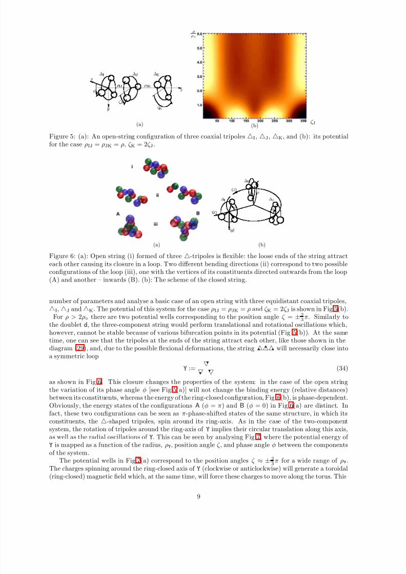
◦ ζ J(a) (b)
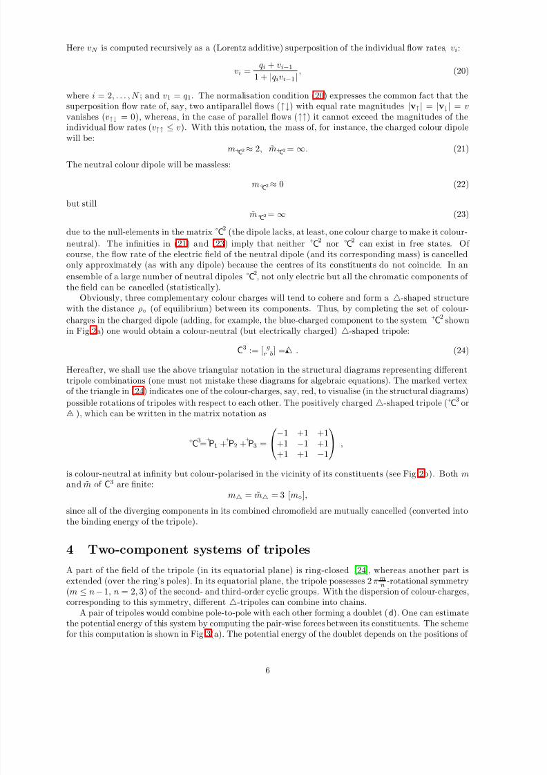
Figure 5: (a): An open-string configuration of three coaxial tripoles △I, △J, △K, and (b): its potentialfor the case ρIJ = ρJK = ρ, ζ K = 2ζ J.
º
º
º
º
º
º
º
º
º
º
º
º
º
º º
º
º
º
º
º
º
º
º
º
º
º
º º
º
º
º
º
º
º
º
º
º
º
º
º
º
º
º
º
º
º
º
º
º
º
º
º
º
º º
º º
º º
º º º º º
º º
º º
º º
º
º
º
º
º
º
º
º
º
º
º
º
º
º
º
º
º
º
º
º
º
º
º
º
º
º
º
º
º
º
º
º
º
º
º
º
º
º
º
º
º
ºº
º º º º º º º º º
ºº
º
º
º
º
º
º
º
º
º
º
º
º
º
º
º
º
º
º
º
º
º
º
º
º
º
º
º
º
º
º
º
º
º
º
º
º
º
º
º
º
º
º
º
º
º
º
º
º
º
º
º
º
º
º
º
º
º
º
º
º
º
º
º
º
º
º
º
º
º
º
º
º
º
º
º
º
º
º
º
º
º
º
º
º
º
º
º
º º
º
º
º º
º º º
º
º º º
º º
º
º
º º
º
º
º
º
º
º
º
º
º
º
º
º
º
º
º
º
º
º
º
º
º
º
º
º
º
º
º
º
º
º
º
º
º
º º º º
ººº
º º º º
º
º
º
º
º
º
º
º
º
º
º
º
º
º
º
º
º
º
º
º
º
º
º
º
º
º
º
º
º
º
º
º
º
º
º
º
º
º
º
º
º
º
º
º
º
º
º
º
º
º
º
º
º
º
º
º
º
º
º
º
º
º
º
º
º
º
º
º
º
º
º
º
º
º
º
º
º
º
º
º
º
º
º º
º
º º
º º º
º
º º º
º º
º
º º
º
º
º
º
º
º
º
º
º
º
º
º
º
º
º
º
º
º
º
º
º
º
º
º
º
º
º
º
º
º
º
º
º
ºº
ººº
ººº
ººº
ºº
º
º
º
º
º
º
º
º
º
º
º
º
º
º
º
º
º
º
º
º º
º
º
º
º
º
º
º º
º
º
º
º
º
º
º
º
º
º
º
º
º
º
º
º
º
º
º
º º º º º º º
º
º
º
º
º
º
º
º
º
º
º
º
º
º
º
º
º
º
º
º
º
º
º
º
º
º
º
º
º
º
º
ºº
ºº
ºº
ººº
ºº
º
º
º
º
º
º
º
º
º
º
º
º
º
º
º
º
º
º
º
º
º
º
º
º
º
º
º
º
º
º
º
º
º
º
º
º
º
º
º
º
º
º
º
º
º
º
º
º
º
º
º
º
º
º
º
º
º
º
º
º
º
º
º
º
º
º
º
º
º
º
º
º
º
º
º
º
º
º
º º
º º º º
º
º º º º
º º
º
º
º
º
º
º
º
º
º
º
º
º
º
º
º
º
º
º
º
º
º
º
º
º
º
º
º
º
º
º
º
º
º
º
º
ºº
º
º º º º º º º
º
ºº
º
º
º
º
º
º
º
º
º
º
º
º
º
º
º
º
º
º
º
º
º
º
º
º
º
º
º
º
º
º
º
º
º
º
º
º
º
º
º
º
º
º
º
º
º
º
º º
º
º º
º º º º º º º
º º
º
º º
º
º
º
º
º
º
º
º
º
º
º
º
º
º
º
º
º
º
º
º
º
º
º
º
º
º
º
º
º
º
º
º
º
º
º
º
º
º
º
ºº
º
ºº
º º º º º º º
ºº
º
º
º º
º
º
º
º
º
º
º
º
º
º
º
º
º
º
º
º
º
º
º
º
º
º
º
º
º
º
º
º
º
º
º
º
º
º
º
º
º
º
º
º
º
º
º
º
º
º
º
º
º
º
º
º
º
º
º
º
º
º
º
º
º
º
º
º º
º
º º º
º º º
º º º
º º
º
º
º
º
º
º
º
º
º
º
º
º
º
º
º
º
º
º
º
º
º
º
º
º
º
º
º
º
º
º
º
º
º
º
º
º
º
º
º
º
ºº
º
ºº
ºº
º º º º º º
ºº
º
º
ºº
º
º
º
º
º
º
º
º
º
º
º
º
º
º
º
º
º
º
º
º
º
º
º
º
º
º
º
º
º
º
º
º
º
º
º
º
º
º
º
º
º
º
º
º
º
º
º
º
º
º
º
º
º
º
º
º
º
º
º
º
º
º
º
º
º
º
º
º
º
º
º
º
º
º
º
º
º
º
º
º
º
º
º
º
º
º º º º º º
º º
º
º
º
º
º
º
º
º
º
º
º
º
º
º
º
º
º
º
º
º
º
º
º
º
º
º
º
º
º
º
º
ºº
º º º º º
ºº
º
º
º
º
º
º
º
º
º
º
º
º
º
º
º
º
º
º
º
º
º
º
º
º
º
º
º
º
º
º
º
º
º
º
º
º
º
º
º
º
º
º
º
º
º
º
º
º
º
º
º
º
º
º
º
º
º
º
º
º
º
º
º
º
º
º º
º º
º º º º
º
º º
º
º
º
º
º
º
º
º
º
º
º
º
º
º
º
º
º
º
º
º
º
º
º
º
º
º
º
º
º
º
ºº
º º º º º
ºº
º
º
º
º
º
º
º
º
º
º
º
º
º
º
º
º
º º º º º
º º º º º º º º º º º º º º º
º º º º º
º º º º
º º º º º º º º º º º º
º º º º
º º º º
º º º º
º º º º
º º º º º º º
º º º º º º
Ü µ
Ý µ
º º º º º º º º º
Þ µ
Ö
Ö
Ö
¡
Á
¡
Ã
¡
Â
º º º º
º º º º
º º º º
º º º º
º º º º
º º º º º
º º º º º
º º º º
º º º º º º º º
º º º º º º º º º
º º º º º º º º º º º º º º
º º º º º º º º º º º º º º º º º º º º º º º º º º º º º
º º º º º º º º º º º º º º
º º º º º º º º º º
º º º º º º
º º º º º
º º º º º
º º º º
º º º º º
º º º º º
º º º º
º º º º
º º º º
(a) (b)
Figure 6: (a): Open string (i) formed of three △-tripoles is flexible: the loose ends of the string attracteach other causing its closure in a loop. Two different bending directions (ii) correspond to two possibleconfigurations of the loop (iii), one with the vertices of its constituents directed outwards from the loop(A) and another – inwards (B). (b): The scheme of the closed string.
number of parameters and analyse a basic case of an open string with three equidistant coaxial tripoles,△I, △J and △K. The potential of this system for the case ρIJ = ρJK = ρ and ζ K = 2ζ J is shown in Fig.5(b).For ρ > 2ρ◦ there are two potential wells corresponding to the position angle ζ = ±2
3π. Similarly to
the doublet d, the three-component string would perform translational and rotational oscillations which,however, cannot be stable because of various bifurcation points in its potential (Fig.5(b)). At the sametime, one can see that the tripoles at the ends of the string attract each other, like those shown in thediagram (29), and, due to the possible flexional deformations, the string △ △△ will necessarily close intoa symmetric loop
Y := △
△
△ (34)
as shown in Fig.6. This closure changes the properties of the system: in the case of the open stringthe variation of its phase angle φ [see Fig.5(a)] will not change the binding energy (relative distances)between its constituents, whereas the energy of the ring-closed configuration, Fig.6(b), is phase-dependent.Obviously, the energy states of the configurations A (φ = π) and B (φ = 0) in Fig.6(a) are distinct. Infact, these two configurations can be seen as π-phase-shifted states of the same structure, in which itsconstituents, the △-shaped tripoles, spin around its ring-axis. As in the case of the two-componentsystem, the rotation of tripoles around the ring-axis of Y implies their circular translation along this axis,as well as the radial oscillations of Y. This can be seen by analysing Fig.7, where the potential energy of Y is mapped as a function of the radius, ρY, position angle ζ , and phase angle φ between the componentsof the system.
The potential wells in Fig.7(a) correspond to the position angles ζ ≈ ± 2
3π for a wide range of ρY.
The charges spinning around the ring-closed axis of Y (clockwise or anticlockwise) will generate a toroidal(ring-closed) magnetic field which, at the same time, will force these charges to move along the torus. This
9
8/3/2019 V. N. Yershov- Equilibrium configurations of tripolar charges
http://slidepdf.com/reader/full/v-n-yershov-equilibrium-configurations-of-tripolar-charges 10/22
ρYρ◦
◦ ζ
ρYρ◦
◦ φ(a) (b)
Figure 7: Potential of the three-component closed string Y as a function: (a) of the position angle ζ between the △-constituents of the string; and (b) of their phase angle φ for the fixed ζ = 120◦. Thevertical axes in both plots correspond to radius ρY (in units of ρ◦).
circular motion of charges will generate a secondary (poloidal) magnetic field, contributing to the spinof these charges around the ring-axis, and so forth. The strength of the magnetic field will be covariantwith respect to ρY. The interplay of the varying toroidal and poloidal magnetic fields, oscillating ρY, andvarying velocities of the rotating charges converts this system into a complicated harmonic oscillator witha series of eigenfrequences and oscillatory modes.
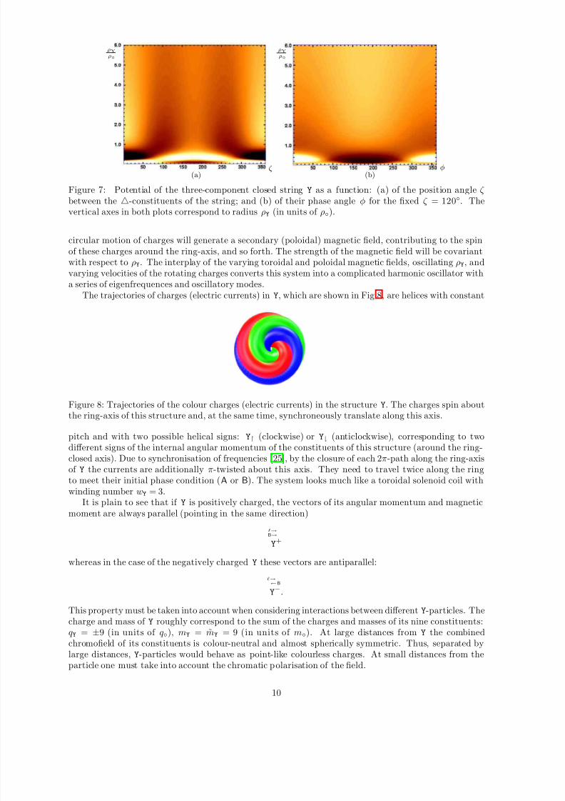
The trajectories of charges (electric currents) in Y, which are shown in Fig.8, are helices with constant
Figure 8: Trajectories of the colour charges (electric currents) in the structure Y. The charges spin aboutthe ring-axis of this structure and, at the same time, synchroneously translate along this axis.
pitch and with two possible helical signs: Y↾ (clockwise) or Y⇂ (anticlockwise), corresponding to twodifferent signs of the internal angular momentum of the constituents of this structure (around the ring-closed axis). Due to synchronisation of frequencies [25], by the closure of each 2π-path along the ring-axisof Y the currents are additionally π-twisted about this axis. They need to travel twice along the ringto meet their initial phase condition (A or B). The system looks much like a toroidal solenoid coil withwinding number wY = 3.
It is plain to see that if Y is positively charged, the vectors of its angular momentum and magneticmoment are always parallel (pointing in the same direction)
ℓ→B→
Y+
whereas in the case of the negatively charged Y these vectors are antiparallel:
ℓ→←B
Y−.
This property must be taken into account when considering interactions between different Y-particles. Thecharge and mass of Y roughly correspond to the sum of the charges and masses of its nine constituents:qY = ±9 (in units of q◦), mY = mY = 9 (in units of m◦). At large distances from Y the combinedchromofield of its constituents is colour-neutral and almost spherically symmetric. Thus, separated bylarge distances, Y-particles would behave as point-like colourless charges. At small distances from theparticle one must take into account the chromatic polarisation of the field.
10
8/3/2019 V. N. Yershov- Equilibrium configurations of tripolar charges
http://slidepdf.com/reader/full/v-n-yershov-equilibrium-configurations-of-tripolar-charges 11/22
6 Chains of unlike-charged tripoles
Hereafter – in order to simplify our analysis – we shall use the observation that △-shaped tripoles, whenclustered, form alike structures on different levels of complexity. For instance, a simple △-tripole and themore complicated ring-closed triplet Y (which consists of three △-tripoles), both possess the same 2
3π-
rotational symmetry. Then (up to a certain limit) one can use the same combinatoric rules when dealingwith structures based on Y- and △-particles. However, some new properties emerging on higher levels of complexity must be taken into account, such as, for example, the helicity property of Y, which by no means
can be found in △. Based on the resemblance between different complexity levels, and using the patternof attraction and repulsion between the tripoles with different positional angles [shown in the diagrams(29) and (30)] , let us explore the variety of possible structures based on the tripolar charges. Of course,the detailed study of these structures and their properties need more rigorous numerical calculations andsimulations, which we shall discuss elsewhere.
Based on the pattern (29) - (30), one can find that the unlike-charged doublets, d− and d+, cancombine and form chains with two possible rotations of the components with respect to each other,clockwise:
d◦2↾ =△− △− △ + △ +
(35)
or anticlockwise:d◦2⇂ =△−△− △ + △ +
, (36)
pole-to-pole to each other. The index “2” refers to the number of doublets involved (d− + d+ → d◦2).The configuration of colour-charges in d◦
2
allows a third doublet (a pair of unlike-charged tripoles) to beattached to the ends of the chain:
d◦3 =△− △−△− △ + △ +
△ +
. (37)
This completes all the three possible 2
3π-rotations of tripoles in the chain. The position angle between
the tripoles at the loose ends of the chain (37) is 180◦, which corresponds to the attractive force betweenthese tripoles [see the diagram (29)]. This allows closing the chain into a loop:
△−
△− — △−
△ +
—△ +
△ +
, (38)
the constituents of which can recombine then into a string of three neutral doublets:
d◦3 → 3d◦ =△− △ + △− △ +
△− △ +
. (39)
This restructuring would happen because of the mutual attraction between the unlike-charged tripoles inthe loop (see Fig.4: the position angle ζ = 180◦ between unlike-charged tripoles corresponds to a potentialwell). The string 3d◦ must be unstable, but a longer chain of the tripole-antitripole pairs possesses akind of cyclic symmetry that allows its closure into a symmetric stable ring. Indeed, the potential wellextending from ζ = 120◦ to ζ = 240◦ (Fig.4) implies the possibility of the unlike-charged tripoles inthe chain being mutually rotated by 120◦. Depending on the chosen direction of rotation (clockwise oranticlockwise), the chain can have one of two possible patterns of colour charges:
d◦6↾ =△−△+
△ + △ − △−△+
△ +
△ − △−△+
△ + △ −
. . . (40)
or
d◦6⇂ =△−△+ △ + △
−
△−△+ △ + △ −
△− △+ △ + △ −
. . . . (41)
The pattern repeats after each six consecutive links (doublets). The mutual orientation of the like-chargedtripoles in the first and sixth links (their 180◦-position angle) corresponds to the attractive force betweenthem and allows the closure of d◦6 in a hexagonal loop with six tripole-antitripole pairs (hexaplet)
△ −
△−
△+ △ +
—△
− △−
△+
△ +
—△
− △−
△+ △ +
(42)
11
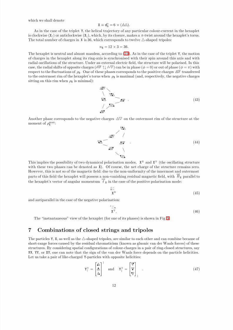
8/3/2019 V. N. Yershov- Equilibrium configurations of tripolar charges
http://slidepdf.com/reader/full/v-n-yershov-equilibrium-configurations-of-tripolar-charges 12/22
which we shall denoteX ≡ d
◦6 = 6 × (△+△−).
As in the case of the triplet Y, the helical trajectory of any particular colour-current in the hexapletis clockwise (X↾) or anticlockwise (X⇂), which, by its closure, makes a π-twist around the hexaplet’s torus.The total number of charges in X is 36, which corresponds to twelve △-shaped tripoles:
nX = 12 × 3 = 36.
The hexaplet is neutral and almost massless, according to (19). As in the case of the triplet Y, the motion
of charges in the hexaplet along its ring-axis is synchronised with their spin around this axis and withradial oscillations of the structure. Under an external electric field, the structure will be polarised. In thiscase, the radial shifts of opposite charges (△+ △ +↑↓△− △ −
) can be in phase (φ = 0) or out of phase (φ = π) withrespect to the fluctuations of ρX. One of these phases corresponds to the positive charges △+ △ +
transferredto the outermost rim of the hexaplet’s torus when ρX is maximal (and, respectively, the negative chargessitting on this rim when ρX is minimal):
△ −
△−
△+ △ +
△ − △−
△+
△ +
△ − △−
△+ △ +
. (43)
Another phase corresponds to the negative charges △− △ −
on the outermost rim of the structure at themoment of ρmax
X:
△ −
△−
△+ △ +
△ − △−
△+
△ +
△ − △−
△+ △ + . (44)
This implies the possibility of two dynamical polarisation modes, X± and X
∓ (the oscillating structurewith these two phases can be denoted as X). Of course, the net charge of the structure remains zero.However, this is not so of the magnetic field: due to the non-uniformity of the innermost and outermost
parts of this field the hexaplet will possess a non-vanishing residual magnetic field, with −→B X parallel to
the hexaplet’s vector of angular momentum−→ℓ X in the case of the positive polarisation mode:
ℓ→B→
X± (45)
and antiparallel in the case of the negative polarisation:
ℓ→←B
X∓. (46)
The “instantaneous” view of the hexaplet (for one of its phases) is shown in Fig .9.
7 Combinations of closed strings and tripolesThe particles Y, X, as well as the △-shaped tripoles, are similar to each other and can combine because of short-range forces caused by the residual chromaticism (known as gluonic van der Waals forces) of thesestructures. By considering spatial configurations of colour-charges in a pair of ring-closed structures, sayXX, YY, or XY, one can note that the sign of the van der Waals force depends on the particle helicities.Let us take a pair of like-charged Y-particles with opposite helicities:
Y+
↾ =
△+
△+△+
↾
and Y+
⇂ =
△ +
△ +
△ +
⇂
. (47)
12
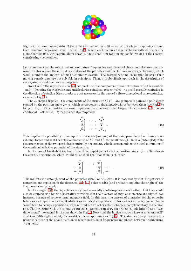
8/3/2019 V. N. Yershov- Equilibrium configurations of tripolar charges
http://slidepdf.com/reader/full/v-n-yershov-equilibrium-configurations-of-tripolar-charges 13/22
Figure 9: Six-component stringX
(hexaplet) formed of the unlike-charged tripole pairs spinning aroundtheir common ring-closed axis. Unlike Fig.8, where each colour charge is chown with its trajectoryalong the ring axis, the diagram above shows a “snap-shot” ( instantaneous configuration) of the chargesconstituting the hexaplet.
Let us assume that the rotational and oscillatory frequencies and phases of these particles are synchro-nised. In this regime the mutual orientation of the particle constituents remains always the same, whichwould simplify the analysis of such a combined system. The systems with no correlation between theirmoving constituents are not solvable in principle. Then, a probabilistic approach in the description of such systems would be more appropriate.
Note that in the representation (47) we mark the first component of each structure with the symbols↾ and ⇂ (denoting the clockwise and anticlockwise rotations, respectively) – to avoid possible confusion in
the direction of rotation (these marks are not necessary in the case of a three-dimensional representation,as seen in Fig.6a).The △-shaped tripoles – the components of the structure Y
+
↾ Y+
⇂ – are grouped in pairs and pair-wiselyrotated by the position angle ζ = π, which corresponds to the attractive force between them [see Fig.3(b)for ρ > 2ρ◦]. Thus, besides the usual repulsive force between like-charges, the structure (47) has anadditional – attractive – force between its componets:
⇐△+
△+
△+
↾ → ←
→ ←→ ←
⇒ △ +
△ +
△ +
⇂
. (48)
This implies the possibility of an equilibrium state (merger) of the pair, provided that there are noexternal forces and that the relative momenta of Y+↾ and Y
+
⇂ are small enough. In this (entangled) statethe orientation of the two particles is mutually dependent, which corresponds to the local minumum of the combined effective potential of the structure.
In the case of like-helicities, two of the three triplet pairs have the position angle ζ = π/6 betweenthe constititing tripoles, which would cause their repulsion from each other:
←←
⇐△+
△+△+
↾ → ←
⇒ △ +
△ +
△ +
↾
→→
. (49)
This inhibits the entanglement of the particles with like-helicities. It is noteworthy that the pattern of attraction and repulsion in the diagrams (48)-(49) coheres with (and probably explains the origin of) thePauli exclusion principle.
In the merger (48) the Y-particles are joined co-axially (pole-to-pole) to each other. But they couldalso be coupled side-by-side (laterally) provided that their vectors of angular momenta are aligned, forinstance, because of some external magnetic field. In this case, the pattern of attraction for the oppositehelicities and repulsion for the like-helicities will also be reproduced. This means that every colour chargewould tend to occupy a position always in front of two other colour-charges, complementary to the firstone. The structure with the laterally coupled Y-particles can grow (in principle, indefinitely) as a “two-dimensional” hexagonal lattice, as shown in Fig.10. Note that the lattice is shown here as a “stand-still”structure, although in reality its constituents are spinning (see Fig.8). The stand-still representation ispossible because of the above mentioned synchronisation of frequencies and phases between neighbouringY-particles.
13
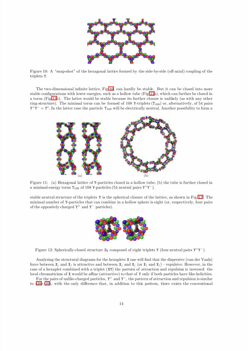
8/3/2019 V. N. Yershov- Equilibrium configurations of tripolar charges
http://slidepdf.com/reader/full/v-n-yershov-equilibrium-configurations-of-tripolar-charges 14/22
Figure 10: A “snap-shot” of the hexagonal lattice formed by the side-by-side (off-axial) coupling of thetriplets Y.
The two-dimensional infinite lattice, Fig.10, can hardly be stable. But it can be closed into morestable configurations with lower energies, such as a hollow tube (Fig.11a), which can further be closed ina torus (Fig.11b). The latter would be stable because its further closure is unlikely (as with any otherring-structure). The minimal torus can be formed of 108 Y-triplets (T108) or, alternatively, of 54 pairsY+Y− = Y
◦. In the latter case the particle T108 will be electrically neutral. Another possibility to form a
(a) (b)
Figure 11: (a) Hexagonal lattice of Y
-particles closed in a hollow tube; (b) the tube is further closed ina minimal-energy torus T108 of 108 Y-particles (54 neutral pairs Y+Y−).
stable neutral structure of the triplets Y is the spherical closure of the lattice, as shown in Fig. 12. Theminimal number of Y-particles that can combine in a hollow sphere is eight (or, respectively, four pairsof the oppositely charged Y
+ and Y− particles).
Figure 12: Spherically-closed structure S8 composed of eight triplets Y (four neutral pairs Y+Y−).
Analysing the structural diagrams for the hexaplets X one will find that the dispersive (van der Vaals)force between X⇂ and X↾ is attractive and between X⇂ and X⇂ (or X↾ and X↾) – repulsive. However, in thecase of a hexaplet combined with a triplet (XY) the pattern of attraction and repulsion is inversed: thelocal chromaticism of X would be affine (attractive) to that of Y only if both particles have like-helicities.
For the pairs of unlike-charged particles, Y+ and Y−, the pattern of attraction and repulsion is similar
to (48)-(49), with the only difference that, in addition to this pattern, there exists the conventional
14
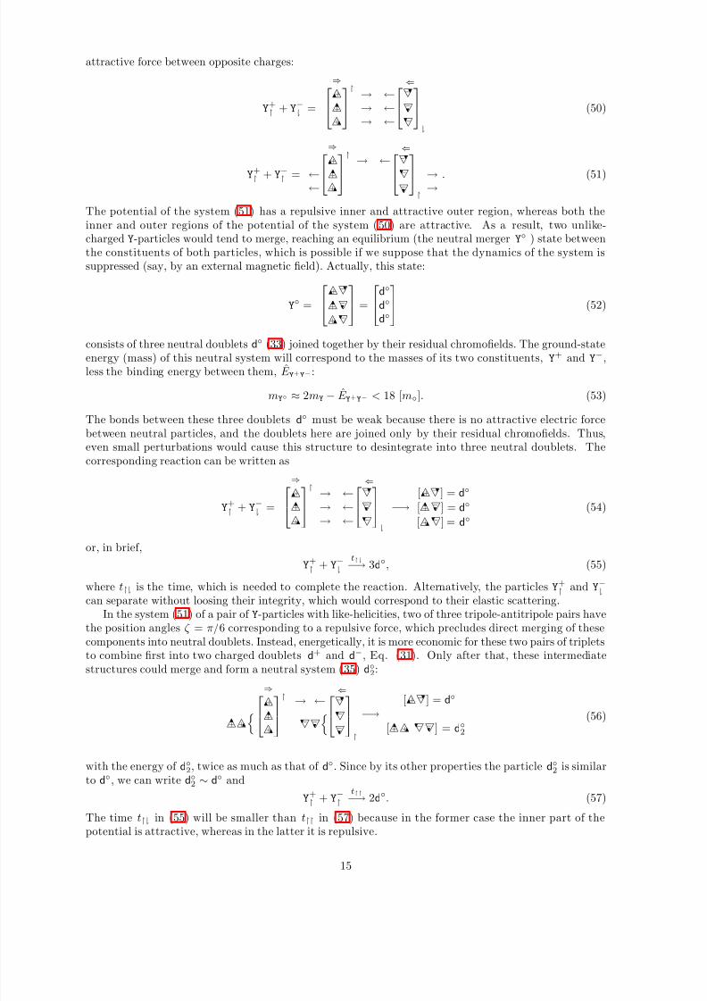
8/3/2019 V. N. Yershov- Equilibrium configurations of tripolar charges
http://slidepdf.com/reader/full/v-n-yershov-equilibrium-configurations-of-tripolar-charges 15/22
attractive force between opposite charges:
Y+↾ + Y
−⇂ =
⇒△+
△+△+
↾ → ←
→ ←→ ←
⇐ △ −
△ −
△ −
⇂
(50)
Y
+↾ + Y
−↾ = ←←
⇒
△+
△+
△+
↾ → ←
⇐
△ −
△ −
△ −
↾
→→ . (51)
The potential of the system (51) has a repulsive inner and attractive outer region, whereas both theinner and outer regions of the potential of the system (50) are attractive. As a result, two unlike-charged Y-particles would tend to merge, reaching an equilibrium (the neutral merger Y
◦ ) state betweenthe constituents of both particles, which is possible if we suppose that the dynamics of the system issuppressed (say, by an external magnetic field). Actually, this state:
Y◦ =
△+
△ −
△+ △ −
△+ △ −
=
d◦d◦d◦
(52)
consists of three neutral doublets d◦ (33) joined together by their residual chromofields. The ground-stateenergy (mass) of this neutral system will correspond to the masses of its two constituents, Y+ and Y
−,less the binding energy between them, E Y+Y− :
mY◦ ≈ 2mY − E Y+Y− < 18 [m◦]. (53)
The bonds between these three doublets d◦ must be weak because there is no attractive electric forcebetween neutral particles, and the doublets here are joined only by their residual chromofields. Thus,even small perturbations would cause this structure to desintegrate into three neutral doublets. Thecorresponding reaction can be written as
Y+
↾ + Y−⇂ =
⇒
△+
△+
△+
↾ → ←→ ←→ ←
⇐
△ −
△ −
△ −
⇂
−→[△+
△ −
] = d◦
[△+ △ −
] = d◦
[△+
△ −
] =d◦
(54)
or, in brief,
Y+
↾ + Y−⇂
t↾⇂−→ 3d◦, (55)
where t↾⇂ is the time, which is needed to complete the reaction. Alternatively, the particles Y+↾ and Y−⇂
can separate without loosing their integrity, which would correspond to their elastic scattering.In the system (51) of a pair of Y-particles with like-helicities, two of three tripole-antitripole pairs have
the position angles ζ = π/6 corresponding to a repulsive force, which precludes direct merging of thesecomponents into neutral doublets. Instead, energetically, it is more economic for these two pairs of tripletsto combine first into two charged doublets d+ and d−, Eq. (31). Only after that, these intermediatestructures could merge and form a neutral system (35) d◦2:
△+ △+
⇒△+
△+△+
↾
→ ← △ − △ −
⇐ △ −
△ −
△ −
↾
−→ [△+ △ −
] = d
◦
[△+ △+
△ − △ −
] = d◦2
(56)
with the energy of d◦2, twice as much as that of d◦. Since by its other properties the particle d◦2 is similarto d◦, we can write d◦2 ∼ d◦ and
Y+
↾ + Y−↾
t↾↾−→ 2d◦. (57)
The time t↾⇂ in (55) will be smaller than t↾↾ in (57) because in the former case the inner part of thepotential is attractive, whereas in the latter it is repulsive.
15
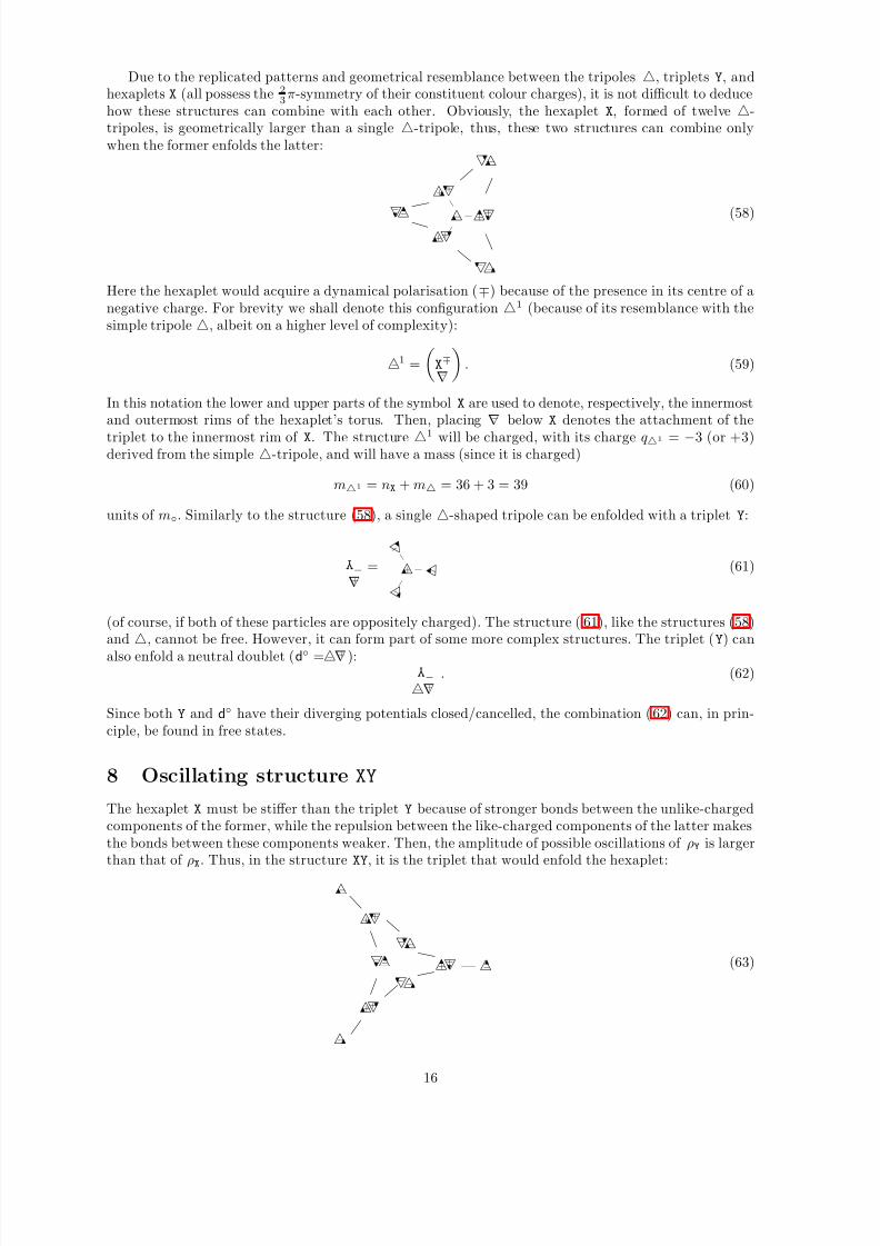
8/3/2019 V. N. Yershov- Equilibrium configurations of tripolar charges
http://slidepdf.com/reader/full/v-n-yershov-equilibrium-configurations-of-tripolar-charges 16/22
Due to the replicated patterns and geometrical resemblance between the tripoles △, triplets Y, andhexaplets X (all possess the 2
3π-symmetry of their constituent colour charges), it is not difficult to deduce
how these structures can combine with each other. Obviously, the hexaplet X, formed of twelve △-tripoles, is geometrically larger than a single △-tripole, thus, these two structures can combine onlywhen the former enfolds the latter:
△ −
△−
△+
△ +
△ − △−
△+
△ +
△ − △−
△+
△ +
–
△− –
– (58)
Here the hexaplet would acquire a dynamical polarisation (∓) because of the presence in its centre of anegative charge. For brevity we shall denote this configuration △1 (because of its resemblance with thesimple tripole △, albeit on a higher level of complexity):
△−1 =
X∓
∇−
. (59)
In this notation the lower and upper parts of the symbol X are used to denote, respectively, the innermostand outermost rims of the hexaplet’s torus. Then, placing
∇− below X denotes the attachment of the
triplet to the innermost rim of X. The structure △1 will be charged, with its charge q△1 = −3 (or +3)derived from the simple △-tripole, and will have a mass (since it is charged)
m△1 = nX + m△ = 36 + 3 = 39 (60)
units of m◦. Similarly to the structure (58), a single △-shaped tripole can be enfolded with a triplet Y:
Y
−
∇+
=
△ −
△−
△−–
△+
–
– (61)
(of course, if both of these particles are oppositely charged). The structure ( 61), like the structures (58)and
△, cannot be free. However, it can form part of some more complex structures. The triplet (Y) can
also enfold a neutral doublet (d◦ =△−∇+ ): Y
−
△−∇+
. (62)
Since both Y and d◦ have their diverging potentials closed/cancelled, the combination (62) can, in prin-ciple, be found in free states.
8 Oscillating structure XY
The hexaplet X must be stiffer than the triplet Y because of stronger bonds between the unlike-chargedcomponents of the former, while the repulsion between the like-charged components of the latter makesthe bonds between these components weaker. Then, the amplitude of possible oscillations of ρY is largerthan that of ρX. Thus, in the structure XY, it is the triplet that would enfold the hexaplet:
△ −
△−
△−
△−
△+ △ +
△ − △−
△+
△ +
△ − △−
△+ △ +
— △− (63)
16
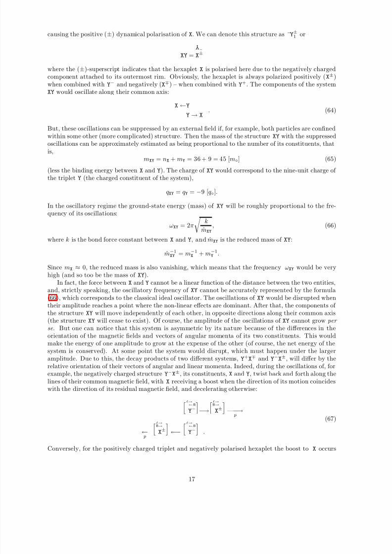
8/3/2019 V. N. Yershov- Equilibrium configurations of tripolar charges
http://slidepdf.com/reader/full/v-n-yershov-equilibrium-configurations-of-tripolar-charges 17/22
causing the positive (±) dynamical polarisation of X. We can denote this structure as −Y±1 or
XY =
Y
−
X±
where the (±)-superscript indicates that the hexaplet X is polarised here due to the negatively chargedcomponent attached to its outermost rim. Obviously, the hexaplet is always polarized positively (X±)when combined with Y
− and negatively (X∓) – when combined with Y+. The components of the system
XY would oscillate along their common axis:
X ←Y
Y → X. (64)
But, these oscillations can be suppressed by an external field if, for example, both particles are confinedwithin some other (more complicated) structure. Then the mass of the structure XY with the suppressedoscillations can be approximately estimated as being proportional to the number of its constituents, thatis,
mXY = nX + mY = 36 + 9 = 45 [m◦] (65)
(less the binding energy between X and Y). The charge of XY would correspond to the nine-unit charge of the triplet Y (the charged constituent of the system),
qXY = qY = −9 [q◦].
In the oscillatory regime the ground-state energy (mass) of XY will be roughly proportional to the fre-quency of its oscillations:
ωXY = 2π
k
mXY
, (66)
where k is the bond force constant between X and Y, and mXY is the reduced mass of XY:
m−1XY
= m−1X
+ m−1Y
.
Since mX ≈ 0, the reduced mass is also vanishing, which means that the frequency ωXY would be veryhigh (and so too be the mass of XY).
In fact, the force between X and Y cannot be a linear function of the distance between the two entities,
and, strictly speaking, the oscillatory frequency of XY cannot be accurately represented by the formula(66), which corresponds to the classical ideal oscillator. The oscillations of XY would be disrupted whentheir amplitude reaches a point where the non-linear effects are dominant. After that, the components of the structure XY will move independently of each other, in opposite directions along their common axis(the structure XY will cease to exist). Of course, the amplitude of the oscillations of XY cannot grow per
se. But one can notice that this system is asymmetric by its nature because of the differences in theorientation of the magnetic fields and vectors of angular momenta of its two constituents. This wouldmake the energy of one amplitude to grow at the expense of the other (of course, the net energy of thesystem is conserved). At some point the system would disrupt, which must happen under the largeramplitude. Due to this, the decay products of two different systems, Y+X∓ and Y
−X±, will differ by the
relative orientation of their vectors of angular and linear momenta. Indeed, during the oscillations of, forexample, the negatively charged structure Y
−X±, its constituents, X and Y, twist back and forth along the
lines of their common magnetic field, with X receiving a boost when the direction of its motion coincides
with the direction of its residual magnetic field, and decelerating otherwise:
ℓ→←B
Y−
−→
ℓ→B→
X±
—−→
p
← p
ℓ→B→
X±
←−
ℓ→←B
Y−
.
(67)
Conversely, for the positively charged triplet and negatively polarised hexaplet the boost to X occurs
17
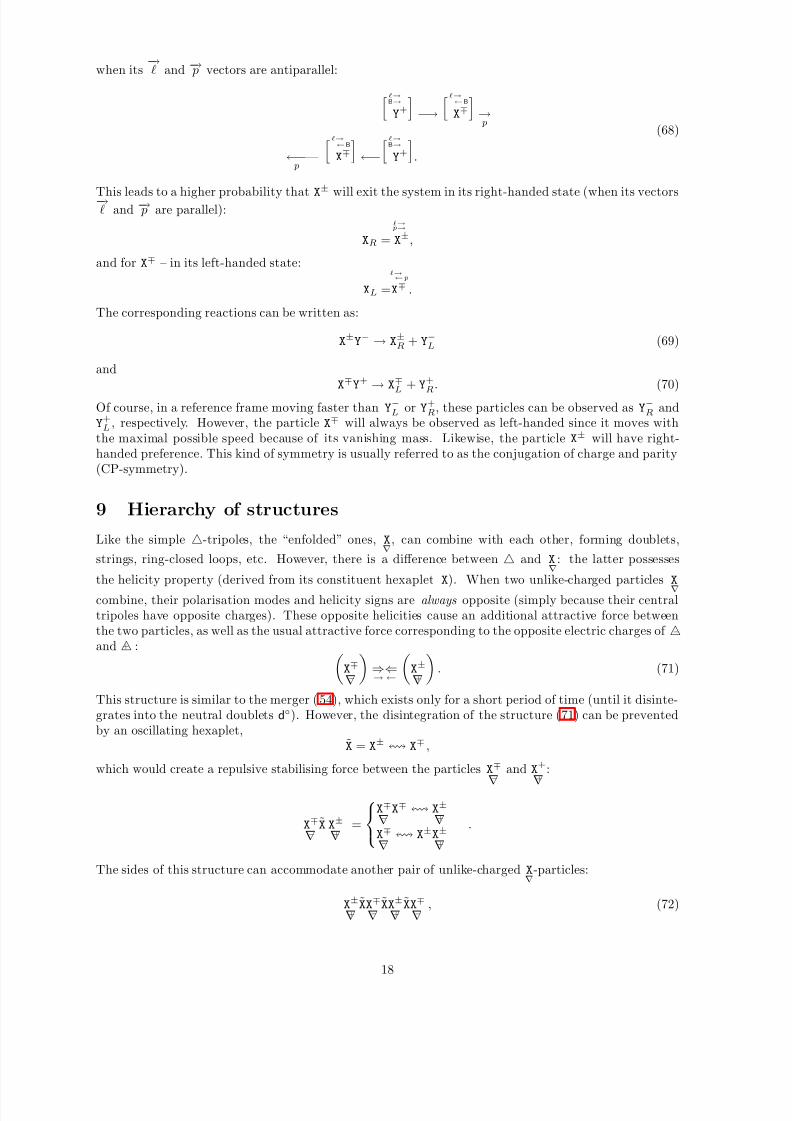
8/3/2019 V. N. Yershov- Equilibrium configurations of tripolar charges
http://slidepdf.com/reader/full/v-n-yershov-equilibrium-configurations-of-tripolar-charges 18/22
when its−→ℓ and −→ p vectors are antiparallel:
ℓ→B→
Y+
−→
ℓ→←B
X∓
→ p
←− p
—
ℓ→←B
X∓
←−
ℓ→B→
Y+
.
(68)
This leads to a higher probability thatX±
will exit the system in its right-handed state (when its vectors−→ℓ and −→ p are parallel):
XR =
ℓ→p→
X±,
and for X∓ – in its left-handed state:
XL =
ℓ→←p
X∓ .
The corresponding reactions can be written as:
X±Y− → X
±R + Y
−L (69)
andX∓Y+
→X∓
L+ Y
+
R. (70)
Of course, in a reference frame moving faster than Y−L or Y
+
R, these particles can be observed as Y−R and
Y+
L , respectively. However, the particle X∓ will always be observed as left-handed since it moves with
the maximal possible speed because of its vanishing mass. Likewise, the particle X± will have right-
handed preference. This kind of symmetry is usually referred to as the conjugation of charge and parity(CP-symmetry).
9 Hierarchy of structures
Like the simple △-tripoles, the “enfolded” ones, X∇
, can combine with each other, forming doublets,
strings, ring-closed loops, etc. However, there is a difference between △ and X∇
: the latter possesses
the helicity property (derived from its constituent hexaplet X). When two unlike-charged particles X
∇combine, their polarisation modes and helicity signs are always opposite (simply because their centraltripoles have opposite charges). These opposite helicities cause an additional attractive force betweenthe two particles, as well as the usual attractive force corresponding to the opposite electric charges of △−and △+ :
X∓
∇−
⇒→
⇐←
X±
∇+
. (71)
This structure is similar to the merger (54), which exists only for a short period of time (until it disinte-grates into the neutral doublets d◦). However, the disintegration of the structure (71) can be preventedby an oscillating hexaplet,
X = X± X
∓ ,
which would create a repulsive stabilising force between the particles X∓
∇−
and X±
∇+
:
X∓
∇−X X
±
∇+=
X∓
∇−X∓ X
±
∇+
X∓
∇− X
±X±
∇+
.
The sides of this structure can accommodate another pair of unlike-charged X∇
-particles:
X±
∇+XX∓
∇−XX±
∇+XX∓
∇−, (72)
18
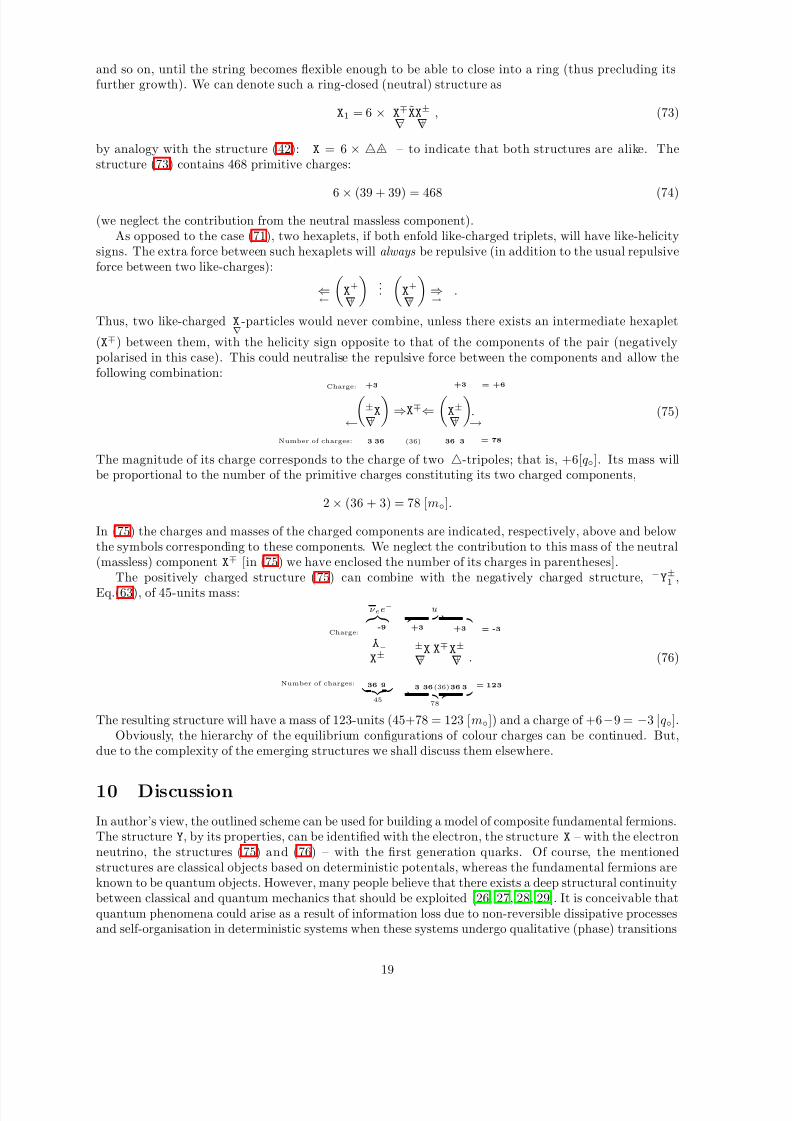
8/3/2019 V. N. Yershov- Equilibrium configurations of tripolar charges
http://slidepdf.com/reader/full/v-n-yershov-equilibrium-configurations-of-tripolar-charges 19/22
and so on, until the string becomes flexible enough to be able to close into a ring (thus precluding itsfurther growth). We can denote such a ring-closed (neutral) structure as
X1 = 6 × X∓
∇−XX±
∇+, (73)
by analogy with the structure (42): X = 6 × △−△+ – to indicate that both structures are alike. Thestructure (73) contains 468 primitive charges:
6 × (39 + 39) = 468 (74)
(we neglect the contribution from the neutral massless component).As opposed to the case (71), two hexaplets, if both enfold like-charged triplets, will have like-helicity
signs. The extra force between such hexaplets will always be repulsive (in addition to the usual repulsiveforce between two like-charges):
⇐←
X±
∇+
...
X±
∇+
⇒→
.
Thus, two like-charged X∇
-particles would never combine, unless there exists an intermediate hexaplet
(X∓) between them, with the helicity sign opposite to that of the components of the pair (negativelypolarised in this case). This could neutralise the repulsive force between the components and allow thefollowing combination:
Charge:
Number of charges:
←
+3
3
±X
∇+
⇒
36
X∓
(36)
⇐X±
∇+
36
+3
3
= +6
= 78
→. (75)
The magnitude of its charge corresponds to the charge of two △-tripoles; that is, +6[q◦]. Its mass willbe proportional to the number of the primitive charges constituting its two charged components,
2 × (36 + 3) = 78 [m◦].
In (75) the charges and masses of the charged components are indicated, respectively, above and belowthe symbols corresponding to these components. We neglect the contribution to this mass of the neutral(massless) component X∓ [in (75) we have enclosed the number of its charges in parentheses].
The positively charged structure (75) can combine with the negatively charged structure, −Y±1 ,
Eq.(63), of 45-units mass:
Charge:
Number of charges:
νee− Y
−
X±
36
-9
9 45
u +3
3
±X
∇+
36
X∓
(36)
X±
∇+
36
+3
3 78
= -3
= 123
. (76)
The resulting structure will have a mass of 123-units (45+78 = 123 [m◦]) and a charge of +6−9 = −3 [q◦].Obviously, the hierarchy of the equilibrium configurations of colour charges can be continued. But,
due to the complexity of the emerging structures we shall discuss them elsewhere.
10 Discussion
In author’s view, the outlined scheme can be used for building a model of composite fundamental fermions.The structure Y, by its properties, can be identified with the electron, the structure X – with the electronneutrino, the structures (75) and (76) – with the first generation quarks. Of course, the mentionedstructures are classical objects based on deterministic potentals, whereas the fundamental fermions areknown to be quantum objects. However, many people believe that there exists a deep structural continuitybetween classical and quantum mechanics that should be exploited [26, 27, 28, 29]. It is conceivable thatquantum phenomena could arise as a result of information loss due to non-reversible dissipative processesand self-organisation in deterministic systems when these systems undergo qualitative (phase) transitions
19
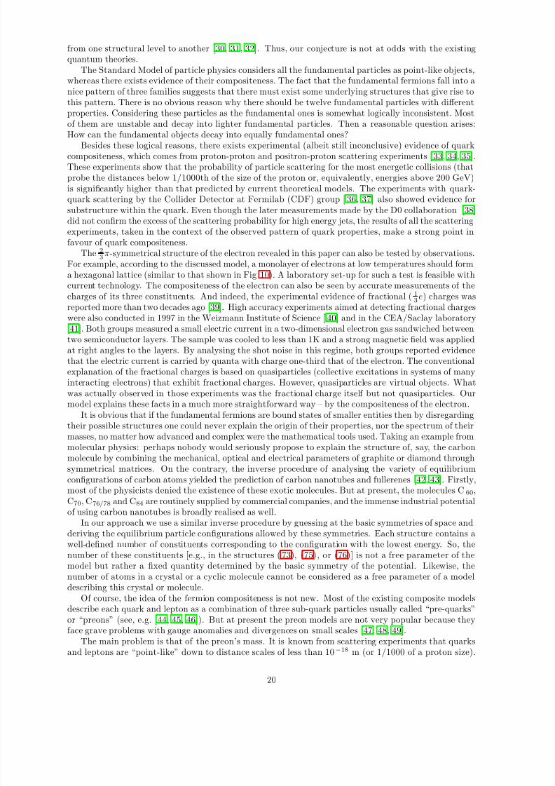
8/3/2019 V. N. Yershov- Equilibrium configurations of tripolar charges
http://slidepdf.com/reader/full/v-n-yershov-equilibrium-configurations-of-tripolar-charges 20/22
from one structural level to another [30, 31, 32]. Thus, our conjecture is not at odds with the existingquantum theories.
The Standard Model of particle physics considers all the fundamental particles as point-like objects,whereas there exists evidence of their compositeness. The fact that the fundamental fermions fall into anice pattern of three families suggests that there must exist some underlying structures that give rise tothis pattern. There is no obvious reason why there should be twelve fundamental particles with differentproperties. Considering these particles as the fundamental ones is somewhat logically inconsistent. Mostof them are unstable and decay into lighter fundamental particles. Then a reasonable question arises:
How can the fundamental objects decay into equally fundamental ones?Besides these logical reasons, there exists experimental (albeit still inconclusive) evidence of quarkcompositeness, which comes from proton-proton and positron-proton scattering experiments [33, 34, 35].These experiments show that the probability of particle scattering for the most energetic collisions (thatprobe the distances below 1/1000th of the size of the proton or, equivalently, energies above 200 GeV)is significantly higher than that predicted by current theoretical models. The experiments with quark-quark scattering by the Collider Detector at Fermilab (CDF) group [ 36, 37] also showed evidence forsubstructure within the quark. Even though the later measurements made by the D0 collaboration [38]did not confirm the excess of the scattering probability for high energy jets, the results of all the scatteringexperiments, taken in the context of the observed pattern of quark properties, make a strong point infavour of quark compositeness.
The 2
3π-symmetrical structure of the electron revealed in this paper can also be tested by observations.
For example, according to the discussed model, a monolayer of electrons at low temperatures should form
a hexagonal lattice (similar to that shown in Fig.10). A laboratory set-up for such a test is feasible withcurrent technology. The compositeness of the electron can also be seen by accurate measurements of thecharges of its three constituents. And indeed, the experimental evidence of fractional ( 1
3e) charges was
reported more than two decades ago [39]. High accuracy experiments aimed at detecting fractional chargeswere also conducted in 1997 in the Weizmann Institute of Science [ 40] and in the CEA/Saclay laboratory[41]. Both groups measured a small electric current in a two-dimensional electron gas sandwiched betweentwo semiconductor layers. The sample was cooled to less than 1K and a strong magnetic field was appliedat right angles to the layers. By analysing the shot noise in this regime, both groups reported evidencethat the electric current is carried by quanta with charge one-third that of the electron. The conventionalexplanation of the fractional charges is based on quasiparticles (collective excitations in systems of manyinteracting electrons) that exhibit fractional charges. However, quasiparticles are virtual objects. Whatwas actually observed in those experiments was the fractional charge itself but not quasiparticles. Ourmodel explains these facts in a much more straightforward way – by the compositeness of the electron.
It is obvious that if the fundamental fermions are bound states of smaller entities then by disregardingtheir possible structures one could never explain the origin of their properties, nor the spectrum of theirmasses, no matter how advanced and complex were the mathematical tools used. Taking an example frommolecular physics: perhaps nobody would seriously propose to explain the structure of, say, the carbonmolecule by combining the mechanical, optical and electrical parameters of graphite or diamond throughsymmetrical matrices. On the contrary, the inverse procedure of analysing the variety of equilibriumconfigurations of carbon atoms yielded the prediction of carbon nanotubes and fullerenes [42, 43]. Firstly,most of the physicists denied the existence of these exotic molecules. But at present, the molecules C60,C70, C76/78 and C84 are routinely supplied by commercial companies, and the immense industrial potentialof using carbon nanotubes is broadly realised as well.
In our approach we use a similar inverse procedure by guessing at the basic symmetries of space andderiving the equilibrium particle configurations allowed by these symmetries. Each structure contains awell-defined number of constituents corresponding to the configuration with the lowest energy. So, thenumber of these constituents [e.g., in the structures (73), (75), or (76)] is not a free parameter of themodel but rather a fixed quantity determined by the basic symmetry of the potential. Likewise, thenumber of atoms in a crystal or a cyclic molecule cannot be considered as a free parameter of a modeldescribing this crystal or molecule.
Of course, the idea of the fermion compositeness is not new. Most of the existing composite modelsdescribe each quark and lepton as a combination of three sub-quark particles usually called “pre-quarks”or “preons” (see, e.g. [44, 45, 46]). But at present the preon models are not very popular because theyface grave problems with gauge anomalies and divergences on small scales [47, 48, 49].
The main problem is that of the preon’s mass. It is known from scattering experiments that quarksand leptons are “point-like” down to distance scales of less than 10−18 m (or 1/1000 of a proton size).
20
8/3/2019 V. N. Yershov- Equilibrium configurations of tripolar charges
http://slidepdf.com/reader/full/v-n-yershov-equilibrium-configurations-of-tripolar-charges 21/22
The momentum uncertainty of a preon (of whatever mass) confined to a box of this size is about 200 GeV,which is 50,000 times larger than the mass of the up-quark. Thus, the problem consists in reconcilingthe relatively small quark masses with the many orders of magnitude greater mass-energies arising fromthe preons’ enormous momenta.
One way in which the mass from internal momentum can be cancelled is to postulate an extremelystrong force, which must be at least 105 times stronger than the strong interaction. It is somewhatunwelcome because it would add a considerable complication to the Standard Model, which already hastoo many arbitrary parameters. However, with such a hyperforce, the preons would be so tightly bound
inside a quark that the energy contribution from their large momentum would be cancelled by their largebinding energy. This approach is quite promising, and that is why we adhere to it in this paper.We have also assumed that infinite energies are not accessible in nature. Then, since it is an experi-
mental fact that energy usually increases as distance decreases, we hypothesize that energy of any fieldon small scales, after reaching a maximum, decays to zero at the origin. With this approach, one can useclassical (intrinsically anomaly-free) potentials on small scales without being troubled by infinite energiesor anomalies.
References
[1] A.Lyubartsev, A.Laaksonen: Chem. Phys. Lett. 325 (2001) 15-22
[2] A.V.Burenin: Physics-Uspekhi 45 (2002) 753–776
[3] C.-H.Sow, et al.: Phys.Rev. A 80 (1998) 2693
[4] A.Wallraff et al.: Nature 425 (2003) 155–158
[5] J.B.Adams et al.: J. Nucl. Materials 216 (1994) 265–274
[6] D.L.Blair, T.Neicu, and A. Kudrolli: Phys. Rev. E 67 (2003) 031303
[7] D.Leckband: Ann. Rev. Biophys. Biomol. Struct. 29 (2000) 1–26
[8] C.J.Crocker, D.G.Grier: Phys. Rev. Lett. 77 (1996) 1897–1900
[9] G.Malescio et al.: J. Phys.: Condens. Matter 14 (2002) 2193–2200
[10] J. Tersoff: Phys. Rev. B 37 (1988) 6991[11] E.F.Suisso, J.P.B.C.de Melo, T.Frederico: Phys. Rev. D 65 (2002) 094009
[12] LEP collaboration: Phys. Lett. B 276 (1992) 247–253
[13] D.Diakonov, V.Petrov, M.Polyakov: Z. Phys. A 359 (1997) 305–314
[14] CDF collaboration: Phys. Rev. Lett. 74 (1995) 2626–2631
[15] D0 collaboration: Phys. Rev. Lett. 74 (1995) 2632–2637
[16] V.V.Barmin et al.: (DIANA collaboration), Yad. Fiz. 66 (2003) 1763–1766
[17] R.M.Santilli, D.D.Shillady: Int. J. Hydr. Energy 24 (1999) 943–956
[18] R.Eisberg, R.Resnick: Quantum physics of atoms, molecules, solids, nuclei, and particles, 2nd ed.,“John Wiley & Sons, Inc.” (1985) 618–631
[19] A.Grutsch, F.Herrmann: Eur. J. Phys. 16 (1995) 271–274
[20] G. Martens et al.: Eur. Phys. J. A 18 (2003) 223–226
[21] M.C.Birse: Progr. Part. Nucl. Phys. 25 (1990) 1–80
[22] H.-J.Pirner: Prog. Part. Nucl. Phys. 29 (1992) 33–85
[23] P.O.Bowman, A.P.Szczepaniak, Phys. Rev. D 70 (2004) 016002
21
8/3/2019 V. N. Yershov- Equilibrium configurations of tripolar charges
http://slidepdf.com/reader/full/v-n-yershov-equilibrium-configurations-of-tripolar-charges 22/22
[24] M.Kibler, G.-H.Lamot, P.Winternitz: Int. J. Quant. Chem. 43 (1992) 625
[25] H.F.El-Nashar et al.: Chaos 13 (2003) 1216–1225
[26] P.A.M.Dirac: Rev.Mod.Phys., 17 (1945) 195–199
[27] P.A.M.Dirac: Sci.Am., 208 (1963) 45-53
[28] A. Mostafazadeh: Phys.Rev. A 60 (1999) 5144–5145
[29] C.K.Raju: Found. of Phys. 34 (2004) 937–962
[30] G.’t Hooft: Class. Quantum Gravity, 16 (1999) 3263–3279
[31] G.’t Hooft: Quantum Mechanics and Determinism , Preprint: hep-th/0105105 (2001) 13 p.
[32] I.Prigogine, T.Petrovsky, G.Ordonez: in Proc. 24-th IHEP Workshop, ed. V.A.Petrov (IHEP Press,Protvino 2001) 204–220
[33] E.J.Eichten, K.D.Lanc, M.E.Peskin: Phys. Rev. Lett 50 (1983) 811–814
[34] C.Adloff et al. (HERA collab.): Zeitschrift f. Physik. C 74 (1997) 191–205
[35] J.Breitweg et al. (ZEUS collab.): Zeitschrift f. Physik. C 74 (1997) 207–220
[36] F.Abe et al. (CDF collaboration): Phys. Rev. Lett., 70 (1993) 1376–1380
[37] F.Abe et al. (CDF collaboration): Phys. Rev. Lett., 77 (1996) 5336–5341
[38] B.Abbott et al. (D0 collaboration): Phys. Rev. D 64 (2001) 032003
[39] G.S.LaRue, J.D.Phillips, W.M.Faiebank: Phys. Rev. Lett. 46 (1981) 967–970
[40] R. de-Picciotto et al.: Nature 389 (1997) 162–164
[41] L.Saminadayar et al.: Phys. Rev. Lett. 79 (1997) 2526–2529
[42] P.M.Ajayan: Chem. Rev. 99 (1999) 1787
[43] P.J.F.Harris: Carbon nanotubes and related structures (Cambridge Univ. Press, Cambridge 1999)
296 p.
[44] J.C.Pati, A.Salam: Phys. Rev. D 8 (1973) 1240–1251
[45] H.Harari, Phys. Lett. B 86 (1979) 83–86
[46] H.Harari, N.Seiberg: Phys. Lett. B 98 (1981) 269–279
[47] S.Weinberg: Phys. Rev. D 13 (1976) 974
[48] J.-J.Dugne: Higgs pain? take a preon! , Preprint: hep-ph/9709227 (1997) 13 p.
[49] R.D.Peccei: The mystery of flavour Preprint: hep-ph/9712422 (1997) 23 p.