NASA-CR-199628

/ /

V

t

///

Final Report

for

NASA Cooperative Agreement NCA2-719NASA Ames Research Center

Numerical Simulation of Supersonic and Hypersonic Inlet Flow Fields

(NASA-CR-1996ZS) NUMERICAL N96-13017

SIMULATION OF SUPERSONIC ANO

HYPERSONIC INLET FLO_ FIELCS Final

Report (North Carolina State Unclas

Univ.) 4C p

G3/02 0067496

D. Scott McRaeDean A. Kontinos

Mars Mission Research Center

North Carolina State UniversityRaleigh, North Carolina

July 21, 1995

https://ntrs.nasa.gov/search.jsp?R=19960003008 2018-06-17T08:16:42+00:00Z

ABSTRACT

Thisreportsummarizestheresearchperformedby NorthCarolinaStateUniversity andNASA Ames Research Center under Cooperative Agreement NCA2-719, "Numerical

Simulation of Supersonic and Hypersonic Inlet Flow Fields". Four distinct rotated upwindschemes were developed and investigated to determine accuracy and practicality. The schemefound to have the best combination of attributes, including reduction to grid alignment with norotation, was the cell centered non-orthogonal (CCNO) scheme. In 2-D, the CCNO scheme

dramatically improved accuracy when used with first order flux interpolation. CCNO alsoimproved rotation when flux interpolation was extended to second order. In 3-D,improvements were less dramatic in all cases, with second order flux interpolation showing theleast improvement over grid aligned upwinding. The reduction in improvement is attributed touncertainly in determining optimum rotation angle and difficulty in performing accurate andefficiently interpolation angle in 3-D. The CCNO rotational technique will prove very usefulfor increasing accuracy when second order interpolation is not appropriate and will materially

improve inlet flow solutions.

INTRODUCTION

The development programs of the High Speed Civil Transport, National AerospacePlane, and next generation fighter/attack aircraft have identified the need for greaterunderstanding and predictive capability of the complex fluid dynamic processes occumng inhigh speed inlet configurations. The flow fields in the inlet are replete with intricate fluidphenomena such as crossing shock waves, shock-wave/turbulent-boundary-layer interactions,merging comer flow boundary layers, and vortical flow. Because of limitations in wind tunnelcapabilities such as limitations of scale and in non-obtrusive measuring techniques, much of theunderstanding of inlet flowfields is a result of numerical simulation. These computer solutionsrely heavily on state-of-the-art numerical techniques.

A commonly and confidently used numerical procedure is the upwind scheme whichhas been a major breakthrough in the modeling of fluid flow in the transonic through

hypersonic flow regimes. The upwind schemes have provided the ability to capture flowdiscontinuities within a few grid points without tuning the artificial dissipation. However, it iswell known that excess dissipation is generated by upwind schemes when the captureddiscontinuities are oblique to the computational grid. The excess dissipation smears the

captured shock waves, thereby reducing the accuracy of the numerical predictions. High speedinlet configurations are especially prone to this effect because the grid topologies are naturally

h-type configurations with oblique crossing shock waves, reflecting shock waves, and shock-wave/boundary-layer interactions. Thus it is the objective of this research to develop anumerical model that improves the prediction and resolution of these dominant flow features inregions where they are captured oblique to the computational mesh and thereby improve theaccuracy of the global inlet solution.

A promising approach to reducing the aforementioned smearing effect is employing arotated upwind scheme. The rotated upwind procedure is one of a class of newly dev.elopingnumerical procedures that attempt to introduce multi-dimensional dependency into thenumerical integration. The basic idea of the rotated upwind scheme is to dynamically align theupwind difference stencil in a direction based on the developing flow field features. Thisprocedure is an alternative to traditional schemes where the dissipation model is affixed by thecomputational mesh. The realignment of the upwind operator enhances the ability of thecomputational model to predict more accurately the local flow physics. The rotation isespecially beneficial in regions where a dominant flow feature, such as a shock wave, existsand is oblique to the computational grid. As mentioned previously, these features commonly

occur in high speed inlet simulations.

A focused investigationwas conducted under thiscooperativeagreement to determine

how the rotation could best be performed and to ascertain how rotation improves the

computational results. Rather than repeat published explanations and data, a review of the

techniques developed and results obtained is presented below and two AJAA papers whichinclude detailed explanations and results are included as appendices. These papers include

brief reviews of previous rotation and multidimensional upwind research, including references.

RESEARCH RESULTS

Several rotated upwind schemes have been developed for the Euler equations in twodimensions, all of which show significantly improved shock capturing ability over grid aligned

schemes to first-order accuracy when the shock wave is oblique to the grid. It is initiallyunclear which of the schemes offer the best promise for further development. Therefore an

initial study is performed where the essential differences between the previous schemes aredistilled and then used as building blocks for competing baseline algorithms. This step of theresearch resulted in four, fh'st-order accurate, rotated upwind schemes that are presented in

AIAA Paper 94-0079 "Rotated Upwind Strategies for Solution of the Euler Equations", a copyof which is attached. The four baseline schemes are the result of a two parameter survey ofalgorithm characteristics. The parameters are the position in the cell at which the rotation takesplace (cell-center vs. cell-edge) and the topological space in which the rotation takes place(physical vs. computational). It is found that the cell-center rotation strategies are more robustand accurate than the ceil-edge schemes because of a requisite averaging procedure in the cell-

center schemes. The averaging procedure acts as an inherent smoothing agent and eliminatesodd-even decoupling which is found to be characteristic of the ceil-edge schemes. It is alsoshown that rotating in computational space vs. a rotation in physical space is simpler toimplement and has the advantage that it will revert to a grid aligned formulation. It is alsoshown that the fast-order accurate rotated scheme produces results typical of the second-orderaccurate grid aligned scheme for the solution of a two-dimensional reflecting shock wave ductconfiguration.

The comparative study noted above revealed that a baseline fast-order accurate rotatedupwind scheme where the rotation in computational space is performed at each ceil-center anddesignated as CCNO (Cell Center rotation, Non-Orthogonal fluxes) has the best overallcharacteristics. The scheme was then extended to second-order accuracy and viscous termswere included to model the Navier-Stokes equations. Furthermore, rotated boundaryconditions were also developed. The extended algorithm was applied to various shockreflection and shock-boundary layer interaction flowfields. The results are contained in AIAAPaper 94-2291, "Rotated Upwind Algorithms for Solution of Two- and Three-DimensionalEuler and Navier-Stokes Equations" which is attached. The first test case, that of an inviscidshock wave reflection demonstrates that the CCNO algorithm yields a more accurate result than

the grid aligned scheme to both first- and second-order accuracy. Furthermore, the improvedaccuracy is maintained as the grid density is increased. This result is an improvement overprevious rotated schemes which show only marginal improvement to second-order accuracy.The next test case is a shock wave impinging on a turbulent boundary layer. To first-orderaccuracy, the CCNO scheme is shown to produce results in better agreement with theexperimental data as compared to the grid aligned scheme. To second-order accuracy, althoughthe inviscid region of the flowfield is qualitatively improved with the CCNO scheme, noimprovement in the wall pressure and skin friction distributions are realized. This result is notunexpected, as the mathematical character of the governing equations changes from essentiallyhyperbolic outside the viscous layer to essentially parabolic near the surface. Therefore despitethe improved prediction in the inviscid region, the wall properties are dominated by the viscousterms prediction which are inherently elliptical in nature and thereby do not benefit fromupwinding. Although this is a disappointing result in terms of wall predictions, it is

encouraging in terms of interior flow measurements such as mass flow rates and thrust

performance which are integrated quantities across the entire domain.

The two-dimensional CCNO algorithm was extended to three dimensions and is also

described in the previously cited paper. The key development made during the extension of the

algorithm was the derivation of two sequences of rotation that align a coordinate axis in anygiven preferred direction. Furthermore, the sequences of coordinate rotation are designed totake advantage of directional symmetry such that the number of possible orientations of therotated coordinate system with respect to the original coordinate system is minimized.Consequently, the logic required in the interpolation and projection procedures is reduced.The result is an automatic method of aligning efficiently a coordinate axis in any given or

computed preferred direction.

The three-dimensional algorithm is shown to be sufficiently robust to compute complexflowfields commonly found in supersonic through hypersonic inlet configurations. An inviscidthree-dimensional shock surface reflection test case shows that the CCNO algorithm improvesthree-dimensional shock wave capturing to both first- and second-order accuracy. This is a

significant result in light of other recent multi-dimensional algorithms that show only marginalor no improvement to three-dimensional inviscid calculations. However, it is also shown thatthe accuracy improvements in the three-dimensional calculation are not as great as what wasseen in two dimensions. It is believed that this is a result of uncertainties in selecting a true

dominant direction which becomes more problematic in three dimensions as compared to twodimensions. Viscous calculations of an intersecting-wedge,/corner-flow geometry and a

generic hypersonic inlet configuration (the inlet results are contained in Kontinos, D. A."Rotated Upwind Algorithms for Solution of the Two- and Three-Dimensional Euler andNavier-Stokes Equations," Ph.D. Dissertation, Department of Mechanical and Aerospace

Engineering, North Carolina State University, Raleigh, NC, 1994) show that as in the two-dimensional viscous calculations, the inviscid portion of the flowfield, e.g., the shock waves,

are qualitatively improved using the CCNO algorithm. However to fu'st-order accuracy, thepredictions of pressure and heat transfer on the wall are not improved using the rotatedalgorithm. To second-order accuracy, there is some improvement in the wall propertyproperties in regions of a dominant cross flow feature. For instance, in the intersecting wedgecase better agreement with the experimental data is achieved with the CCNO algorithm in thecross-flow reattachment region of the multiple shock wave structure in the comer of thegeometry. Similar improvement is seen in the generic inlet configuration in the region where

the boundary layer is rolled into a comer vortex.

The accuracy improvements gained by the CCNO algorithm come at a considerablecost. Both the two- and three-dimensional algorithms are shown to consume 2-4 times more

computer time than their grid aligned counterparts. The increase in computer usage is causedby an increase in the work required per iteration and a reduced stability limit which causes anincrease in the number of iterations for convergence. However, regions of potential algorithm

improvement are highlighted that may reduce the work load, such as a more accurate temporallinearization and a simplification of the interpolation procedure. It is believed that the CCNOscheme may have application for inviscid flow solutions but the scheme is immature forviscous flowfields. In viscous flowfields, selection of a dominant direction becomes uncertain

in subsonic regions such as in boundary layers, especially in three dimensions. Moreover, the

fine grid spacing typical of viscous flow field meshes restricts and allowable time step andincreases the amount of computer usage. As mentioned previously, a more accurate temporallinearization may overcome this difficulty. Finally, current research into truly multi-dimensional Riemann solvers may reveal an optimum upwind direction in the boundary layer

thereby refining the CCNO schemes effectiveness.

CONCLUSIONS

The development and evaluation of rotated upwind procedures revealed that bothaccuracy and practicality must be considered in the choice of such schemes. The rotationscheme that was chosen, CCNO, was the best compromise between accuracy and ease of

implementation. This scheme was demonstrated to improve results in essentially inviscid flowregimes in both 2-D and 3-D. The improvement was most dramatic when a first order accuraterotation was used, producing results that compared well with second-order accurate grid

aligned solutions. The second order CCNO scheme also gave improved results over secondorder grid aligned results. However, the improvement was not as dramatic in 3-D and wasachieved at considerable computational cost. Further research is indicated to determine howbest to f'md the optimum upwinding direction in 3-D and how to obtain efficiently interpolatedflux quantities in the rotated directions. The lack of improvement due to rotation in the viscouslayer is forecast by the mathematical character of the governing equations in this region.

RECOMMENDATIONS

CCNO may be used to increase accuracy to match second order grid aligned resultswith only In'st order flux interpolation. This may be particularly useful when the grid isdistorted to conform to geometry or flow features.

Further research should be conducted to optimize rotation direction and to improvehigher order flux interpolation, particularly in 3-D.

AIAA paper 94-0079

32nd Aerospace Sciences Meeting

Reno, NV

Rotated Upwind Strategies for Solution of the

D_,. Kontinos* and D.S. McRavt

North Carotina State UulvermtyRaleigh,North Carolina

Euler EquatlonJ

Four finite volume, fully conservative, rotund upwind

strategies for solution of the two-dimensional Eulerequations are compared. The four strategies are based on thecombinations of two options which are a cell-edge vs. acell-center rotation, and a rotation in physical space vs.

computational space. The four schemes are implementedwith maximum commonalty for direct comparison. Thesolutions are relaxed to steady state by the LU-SGS scheme.Solutions of a Mach 2 channel flow problem are presented

and compared in terms of accuracy and robustness. It isshown that the cell-edge strategies create unacceptableoscillations in the solution while the cell-center strategiescontain inherent smoothing that allow for accurate solutionswith good convergenceproperties.The fn'st-orderrotated

upwind resultsareseentobe comparabletostandardsecond-

orderupwind results.

The development of upwind schemes has been a majorbreakthrough in the modeling of fluid flow in the transonicthrough hypersonic regimes. The upwind schemes haveprovided the ability to capture flow discontinuities within afew grid points without tuning the artificial dissipation.However, it is well known that excess dissipation isgenerated when the captureddiscontinuities axe obliqueto

the grid.

One such upwind algorithm, Rce's 1 scheme, has been

used quite successfully by a variety of researclmrs. The Roescheme models flow discontinuities as a series of linearized

waves. In one dimension, these linearized waves model the

actual wave propagation quite accurately. However, inmultidimensions, the one dimensional Roe scheme

misinterprets the multidimensional flow field andincorrectly models local wave propagation. This manifestsitself as excess dissipation and results in the smearing offlow discontinuities. An excellent discussion of this effect

is presented in Ref. [2].

* Research Assistant, Mechanical and Aerospace

Engineering, Student Member AIAA.t Professor, Mechanical and Aerospace Engineering,Member AIAA.

Copyright © 1994 American Institute of Aeronautics andAsmanantics, Inc. All rights reserved.

In an effort to improve upwind schemes inmultidimensional flow, much recent effort has been focused

on dissipation models that incorporate multidimensional

effects. A comprehensive review by van Leer 3 gives a goodoverview of such methods. One of the approaches is theuse of a rotated upwind scheme. The basic idea is to orientthe upwind solver in a preferred direction (or 'rotate' theintegration stencil to this preferred direction) such that theone dimensional operator can more accurately model themultidimensional flow. Several rotated upwind schemeshave been developed for the Euler equations in two

dimensions(4,5,6,7,8), all of which show significant

improvement over grid aligned schemes to first-orderaccuracy and modest improvement to second-order accuracy.The main drawback of these algorithms has been theincrease in computer work as compared to the grid alignedalgorithms. Moreover, to date a three dimensional

algorithm has not been developed and it is unclear whether arotatedformulation will show the same improvements in3D as it dces in 2D.

The objective of this study is to compare four two-dimensional rotated upwind strategies in terms of accuracyand robustness so that a method can be selected for

development in three dimensions. Each of the strategiescontain elements of previously developed algorithms,

although several aspectsare new. They are implemented

with as much commonalty as possible to promote a goodcomparison.

This study is organized as follows; first Section 2presents the governing equations. Section 3 presents ageneral overview of each of the four strategies. The detailsof the implementation of the smategies axe presented inSection 4. Section 5 will present results of a simplechannel flow problem and Section 6 will conclude.

2.0 The Euler Equations

For this study, the governing equations ate the two-dimensional Euler equations in integral conservation lawform. The setinindexnotationisasfollows:

fpdV+ fp%%dS=OOtvoi s_

BtVot ._f

mass

mom

&Vol surl

energy

In the finite volume framework, the conserved variables axetaken as averages over the cell volume. Thus, the conservedquantifies can be taken out of the volume integrals in theprevious equations. Moreover, the surface integrals becomesummations over the cell sides. Expanding out themomentum equation into its vector components, theequations can be written as,

W = vol. (2.1)

where the conserved variables are,

u=[p pu pv E,]", (2.2)

andthefluxesaregivenby,

p=[: (2.3)

where the cell face normal with magnitude equal to the cell

face length is denoted by ns and the velocity by V. The

variables p, p, u, and v are the pressure, density, and x and yCartesian velocity components, respectively. Using theperfect gas relation, the total energy E t is given by,

p(u 2 + v2)

Et =_-_+ 2 '(2.4)

where 7 is the ratio of specific heats which has a value of1.4 for air.

3.0 Rotated Unwind Strategies

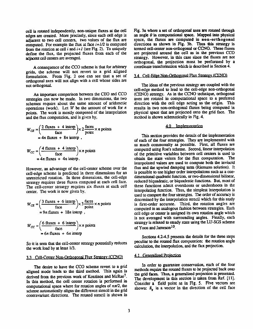
This section presentsan overview of the four strategiescompared in this study. Recall that the main goal of arotated upwind scheme is to align the one dimensionalRiemann solver across flow discontinuities to reduce excessdissipation. In order to achieve this goal, one mustcompute the flux in a direction independent of the grid.This section will describe four strategies for such a fluxcomputation. Each strategy will base the flux computationat the cell edge or cell center, and compute the preferreddirection in physical space or computational space. Thissection describes the strategies in broad terms while Section4 presents the details.

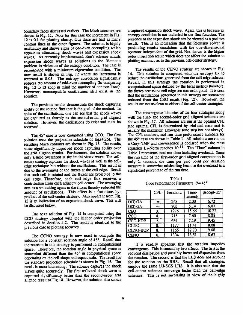
3.1 Cell-Edge Orthogonai Flux Strategy (CEO)

The first strategy is a distillation of the schemedeveloped by Levy, et. al.5. Levy's scheme is a cell-edge

method wherein a preferred upwind direction is selected ateach cell face and two orthogonal fluxes arc computed; anupwind flux in the preferred direction, and a centraldifference flux normal to the preferred direction. This isshown schematically in Fig. 1. Later versions of thealgorithm apply Roe's scheme in both directions 9. Thevalues of the dependent variables are interpolated betweencell centers through a linear-quadratic interpolating function.The rotated flaxes are then projected onto the grid facedirection to ensure conservation. Levy shows improvedshock capturing over grid aligned schemes.

The same strategy is taken by Dadone and Grossman 6.However, a different tactic is used to compute the numericalflux. An upwind flux (Rods scheme) is computed in boththe primary (preferred) and secondary(ca'thogonal)direction.Alsoa simplifiedinterpolationstencilisincorporatedthatessentially 'grabs' the values of the clmmeteristie variables atthe nearest cell center to the rotated stencil. Computationsusing this scheme also show improved results as comparedto grid aligned schemes. Moreover, convergence rate andboundary condition improvements are shown as compared toprevious rotated schemes.

The cell-edge,orthogonal flux philosophy isincorporatedinthisstudyand istermedCEO. An upwindfluxiscomputed in both the preferredand secondarydirectionat each celledge. The interpolationof theprimitivevariablesislinearbetweenadjoiningcells.

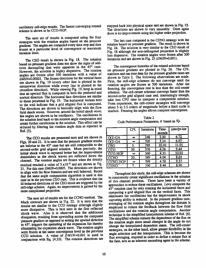
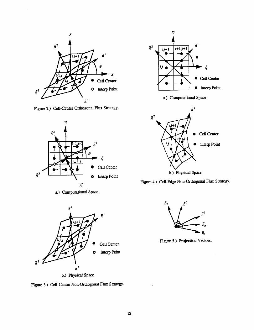
3.2 Cell-Center Ortho2onal Flux Strategy (CCO)

As an alternative to the previous cell-edge strategy, theconcept of a cell-center rotation is now proposed (the notionof assigning a rotation angle to a cell center is recognizedby Davis 4 although a method is not developed). Thissecond strategy, termed cell-center orthogonal or CCO, isderived from the previous rotated finite difference scheme ofKontinos and McRae 7. In this previous work, a rotationangle is selected in computational space thereby def'ming arotated coordinate system. The flux divergence is thencomputed in the rotated frame. The method showsimproved results over grid aligned schemes for both inviscidand viscous flows. Unfortunately, the grid point residualsare computed independently of each other and the scheme isnot conservative as originally implemented.

In order to guarantee conservation, the scheme isconverted from finite difference to finite volume to becomethe CCO strategy. In the CCO scheme, four fluxes arecomputed in two orthogoual directions originating at thecell center (recall in the cell-edge philosophy, twoorthogonal fluxes are computed at each cell face and thenprojectedonto that cell face). These four fluxes are thenprojected around the cell edges, details of which arepresentedin the next section.The CCO strategyisrepresentedin Fig.2 where a singlecellis shownschematicallyalongwiththerotatedfluxes.Becauseeach

cell is rotated independenOy, non-unique fluxes at the celledges are created. More precisely, since each cell edge isadjacent to two cell centers, two values of the flux arecomputed. For example the flux at face i+1/2 is computedfrom the rotation at cell i and i+1 (see Fig. 2). To uniquelydefine the flux, the projected fluxes from each of theadjacentcell centers are averaged.

A consequence of the CCO scheme is that for arbitrarygrids, the scheme will not revert to a grid alignedformulation. From Fig. 2 one can see that a set oforthogonal axes will not align with a cell whose sides arenot orthogonal.

An important comparison between the CEO and CCOstrategies can now be made. In two dimensions, the twoschemes require about the same amount of arithmeticoperations (work). Let W be the amount of work for npoints. The work is mosdy composed of the interpolationand the flux computation, and is given by,

(2 fluxes + 4 interP)x 2 faces xWce face y _ n points

= 4n fluxes + 8n interp ,

Wcc =(4 fluxes +4face interP') xnpoints

= 4n fluxes + 4n interp.

However, an advantage of the cell-center scheme over thecell-edge scheme is predicted in three dimensions for anunrestricted rotation. In three dimensions, the cell-edgestrategy requires three fluxes computed at each cell face.The cell-center strategy requires six fluxes at each cellcenter. The work is now given by,

3 fluxes + 6 )interp . ,_faces .......

= ^ _ ^ ,, _in_Wce face _'_

= 9n fluxes + 18n interp ,

Wcc =(6 fluxes+face6interp') x n p°ints

= 6n fluxes + 6n interp

So it is seen that the cell-center strategy potentially reducesthe work load by at least 1/3.

3.3 Cell-Center Non-Orthogonal Flux Strategy (CCNO)

The desire to have the CCO scheme revert to a gridaligned mode leads to the third method. This again isderived from the previous work of Kontinos and McRae 7.In this method, the cell center rotation is performed incomputational space where for rotation angles of nrJ2, thescheme automatically aligns the difference stencil in the gridcontravariant directions. The rotated stencil is shown in

Hg. 3a where a set of orthogonal axes are rotated throughan angle O in computational space. Mapped into physicalspace, the fluxes are computed in non-orthogonaidirections as shown in Fig. 3b. Thus this strategy istermed cell-center non-orthogonal m"CCNO. These fluxesare projected around the cell as in the previous CCOstrategy. However, in this case since the fluxes are notorthogonal, the projection must be performed by acoordinate transformation which is described in Section 4.

3.4 Cell-Edge Non43rthogonal Flux Strategy (CENO)

The ideas of the previous strategy are coupled with thecell-edge method to lead to the cell-edge non-orthogonal(CENO) strategy. As in the CCNO technique, orthogon_axes arerotatedin computationalspaceto a preferreddirection with the cell edge acting as the origin. Thisresults in two non-orthogonal fluxes being computed inphysical space that are projected onto the grid face. Themethod is shown schematically in Fig. 4.

4.0 Implementation

This section provides the details of the implementationof each of the four strategies. They are implemented withas much commonalty as possible. First, all fluxes arecomputed using Roe's scheme. Second, linear interpolationof the primitive variables between cell centers is used toobtain the state values for the flux computation. Theinterpolated values are used to compute both the inviscidflux and the upwind damping term (Riemann solution). Itis possible to use higher order interpolations such as a one-dimensional quadratic function, _ two-dimensional bilinear,reduced biquadratic, or biquadratic functions. But, most ofthese functions admit overshoots or undershoots in the

interpolating function. Thus, the simplest interpolation isused to compare the four strategies. The order of accuracy isdetermined by the interpolation stencil which for this studyis ftrst-order accurate. Third, the rotation angles arecomputed in an analogous fashion between swategies. Eachcell edge or center is assigned its own rotation angle whichis not averaged with surrounding angles. Finally, eachstrategy is relaxed to steady state using the LU-SGS schemeof Yoon and Jameson 1°.

Sections 4.2-4.5 presents the details for the three stepspeculiar to the rotated flux computation: the rotation anglecalculation, the interpolation, and the flux projection.

4.1 Generalized Projection

In order to guarantee conservation, each of the fourmethods require the rotated fluxes to be projected back ontothe grid faces. Thus, a generalized projection is presented.The development in this section is taken from Ref. [11].Consider a field point as in Fig. 5. Five vectors are

shown: ns is a vector in the direction of the cell face

3

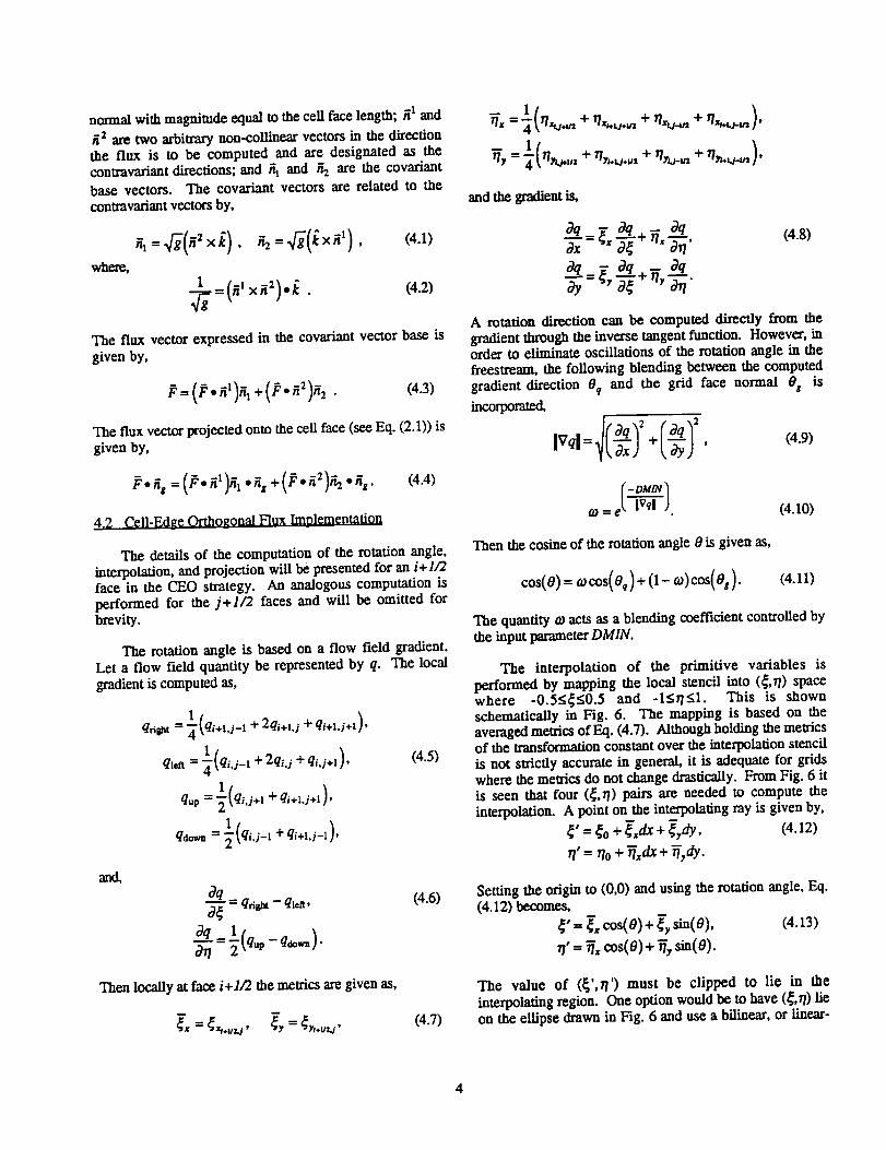
normalwithmagnitudeequaltothecellfacelength;_land

_2 aretwo arbitrarynon-collinearvectorsinthedirectionthefluxis to be computed and are designatedas thecontravariantdirections;and nl and _ arethecovariantbase vectors.The covarlantvectorsaterelatedto the

contravariantvectorsby,

where,1

(4.2)

The fluxvectorexpressedinthecovarlantvectorbaseisgivenby,

(4.3)

The fluxvectorprojectedontothecellface(seeEq.(2.1))isgivenby,

<44)

4.2 Cell-Edge Orthogonal Flux Implementation

The details of the computation of the rotation angle,interpolation, and projection will be presented for an i+I/2face in the CEO strategy. An analogous computation isperformed for the j+]/2 faces and will be omitted forbrevity.

The rotation angle is based on a flow field gradient.Let a flow field quantity be represented by q. The localgradient is computed as,

1 + qi÷Lj+l),qri_t= "_(qi+Lj-1+ 2q/+i.i

Iq,_ = _( q,,j-I+ 2ql,j+ q,,i+l),

1

qup = _'(qi,j+! +q,+L,+,),

1qd,,_n= _(qi.j-I+ qi+l.i-l),

(4.5)

and,

B"-_- qfi_ - ql_,

dq = l-

(4.6)

Thenlocallyat face i+1/2 themetricsaregivenas,

(4.7)

1

1

andthegradientis,

Oq= aq+_ Oq

aq= a_q_ aq0y " +

(4.8)

A rotation direction can be computed directly from thegradient through the inverse tangent function. However, inorder to eliminate oscillations of the rotation angle in thefreestream, the following blending between the computedgradient direction 0q and the grid face normal 0s is

incorporated,

V _q 2

f- DM/N _

= et-r_'). (4.10)

Then thecosineoftherotationangle0isgivenas,

cos(O)=OJcos(Oq)+ (I-_)cos(Oj). (4.11)

The quantity 0) acts as a blending coefficient controlled bythe input parameter DMIN.

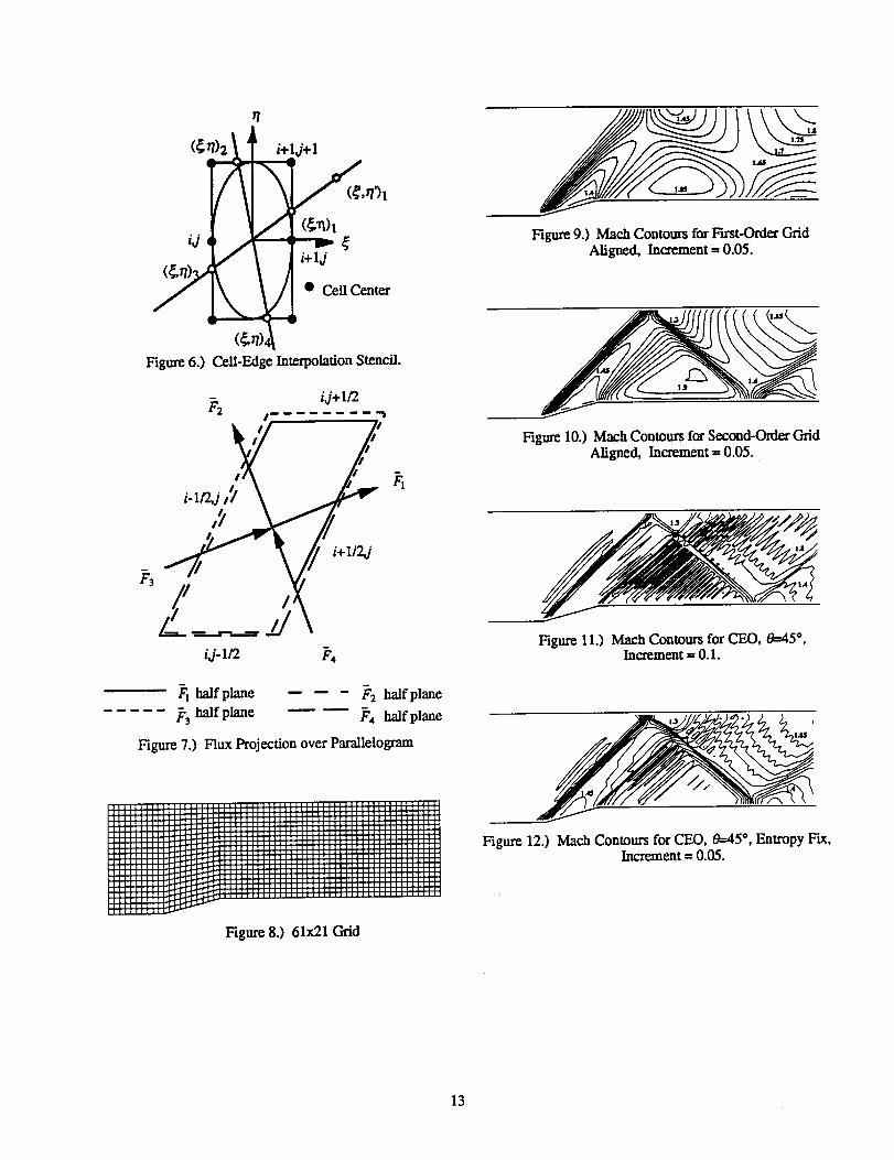
The interpolation of the primitive variables isperformed by mapping the local stencil into (_,r/) spacewhere -0.5<_<0.5 and -1<17<1. This is shownschematically in Fig. 6. The mapping is based on theaveraged metrics of Eq. (4.7). Although holding the metricsof the transformation constant over the interpolation stencilis not strictly accurate in general, it is adequate for gridswhere the metrics do not change drastically. From Fig. 6 itis seen that four (_,_1) pairs are needed to compute theinterpolation. A point on the interpolating my is given by,

_'= _o+ _:dx+ _,dy, (4.12)

71'= no + _':_ + _,#Y.

Setting the origin to (0,0) and using the rotation angle, Eq.(4.12) becomes,

,_'= _'=cos(O)+ _',sin(O), (4.13)

.'= cos(o)+% sin(o).

The value of (_',_1') must be clipped to lie in theinterpolating region. One option would be to have (_,_l) lieon the ellipse drawn in Fig. 6 and use a bilinear, or linear-

4

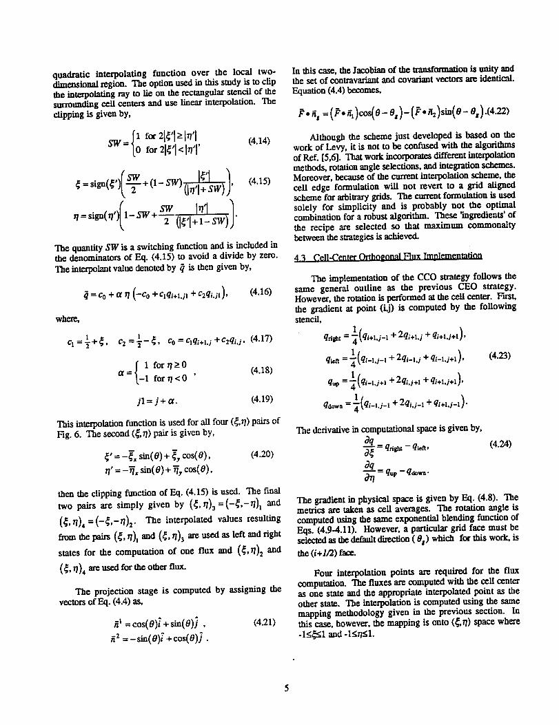
quadraticinterpolating function over the local two-dimensional region. The option used in this study is to clipthe interpolating ray to lie on the rectangular stencil of thesurrounding cell centers and use linear interpolation. Theclipping is given by,

{_for21¢'l_I,71sw= for2]_1<lq1'(4.14)

¢ = sign(_') + (1-SW) (lq' W) '

r/ffi sign(r/,)(l_ SW + SW ,rf, 12 (l_'l+l- sw)

(4.15)

The quantity SW is a switching function and is included inthe denominators of F-xl. (4.15) to avoid a divide by zero.

The interpolant value denoted by ?/is then given by,

_=Co +o_q (-Co +qqi+t.jt +c2qij1), (4.16)

where,

1 lq=T+_, c2=T-_, Co=qqi+l.j+c2qi.j, (4.17)

11 for 7/> 0a= _ fort/<0 ' (4.18)

jl=j+a. (4.19)

This interpolation function is used for all four (_,r/) pairs ofFig. 6. The second (_,_7) pair is given by,

¢'=-_', sin(o)+_,=s(o),_' = -fi, sin(O)+_, cos(o),

(4.20)

then the clipping function of Eq. (4.15) is used. The final

two pairs are simply given by (_,q)3 =(-¢.-_)1 and

(¢'q),=(-¢'-q)2" The interpolated values resulting

fromthe_ (_,r/),and (_,q)3areusedasleftandright

statesforthecomputationof one fluxand (_,7/)2and

(_,_),areusedfortheotherflux.

The projection stage is computed by assigning thevectors of Eq. (4.4) as,

.' =cos(O)_'+_(o)).,_2=-sin(o)f+co.(O)}.

(4.21)

In this case, the Jacobian of the transformation is unity andthe set of contravariant and covariant vectors are identical.Equation (4.4) becomes,

p.,, =(p.,,)cos(o-o, )sin(o-o,).(4.=)Although the scheme just developed is based on the

work of Levy, it is not to be confused with the algorithmsof ReL [5,6]. That work incorporates different interpolationmethods, rotation angle selections, and integration schemes.Moreover, because of the current interpolation scheme, thecell edge formulation will not revert to a grid alignedscheme for arbitrarygrids. The current formulation is usedsolelyfor simplicityand isprobablynot the optimalcombinationfora robustalgorithm.These"ingredients'ofthe recipeare selectedso thatmaximum commonaltybetween the strategies is achieved,

4.3 Cell-Center Orthogonal Flux Implementation

The implementation of the CCO strategy follows thesame general outline as the previous CEO strategy.However, the rotation is performed at the cell center. F'ust,the gradient at point (i,j) is computed by the followingstencil,

1 qi+Lj+t),qright= _'(qi+t,j-I + 2qi+l,j +

1qtea = "_(qi-Ij-1 + 2qi-l.i + q_=l.j+l), (4.23)

1 + qi+lj+x),q,p = _(q_-1._+1 + 2qi.i+l

I + qi+1,j-i)"qdow, = _(qi-lj-I + 2q_j°l

The derivative in computational space is given by,Oq

Oq_"'ff -- qup - qdo_a.

(4.24)

The gradient in physical space is given by Eq. (4.8). Themetrics are taken as cell averages. The rotation angle iscomputed using the same exponential blending function ofEqs. (4.9-4.11). However, a particular grid face must beselected as the default direction (0:) which for this work, is

the (i+I/2) face.

Four interpolation points are required for the fluxcomputation. The fluxes ate computed with the cell centeras one stateand theappropriateinterpolatedpointastheotherstate.The interpolationiscomputedusingthesamemapping methodologygivenintheprevioussection.Inthiscase,however,themappingisonto(_,T/)spacewhere-I<_I and-I<T/_I.

Before the fluxes can be projected, the algorithm mustproperly label each of the four fluxes. This sorting isrequired because the preferred direction may be oriented inany manner with respect to the computationalcoordinates(i.e. grid indices). So to project the "correct" fluxes ontothe cell faces, the fluxes must be ordered. Flux sorting isaccomplished by denoting the first flux counter-clockwise

from cell normal (i+1/2) as the E1 direction (see Fig. 2).The algorithm selects the proper direction by the following_ter_

El. n_.l12j > 0. _1x ff_+u2j > 0. (4.25)

After the _z direction is defined, the other fluxes areincremented in the counter-cleckwise direction.

The last stage of the flux computation is the projectionof the fluxes onto the grid faces. In the CEO method, thetask is straightforward since the rotated fluxes are computedat each cell face and projected onto that face. However forthe CCO method, the set of four fluxes must be projectedaround the entire cell. Such a projection is not unique sotwo methods that are implemented will be outlined.

In the first method, an orthogonal pair of fluxes isassigned to each cell edge. With the notation

_'t =(P._k)tik, (k=l,4), the fluxesat the cell edge are

given as (see Fig. 2),

p,+,,2_=(P,+P.)._,÷,,:,.r:... =(p:+Pl)._,.÷,,:,p,_,,_=(p,+p2)._,_,,2..p,.i_,,_=(p.+p,)._,._.:.

(4.26)

Recall thatunity andidentical.

the fluxes are orthogonal so that the Jacobian isthe contravariant and covariant vectors are

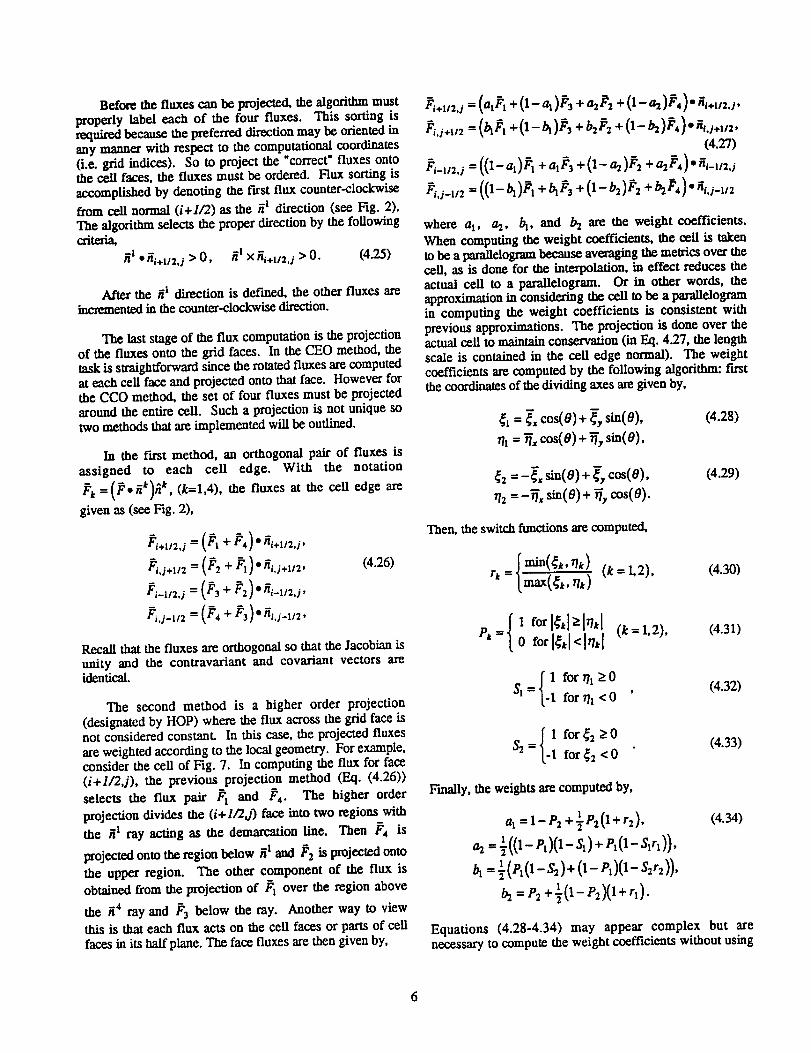
The second method is a higher order projection(designated by HOP) where the flux across the grid face isnot considered constant In this case, the projected fluxesare weighted according to the local geometry. For example,consider the cell of Fig. 7. In computing the flux for face(i+l/2d), the previous projection method (Eq. (4.26))

selects the flux pair Pl and F4. The higher order

projection divides the (i+//2j} face into two regions with

the _i ray acting as the demarcation line. Then F4 is

projected onto the region below _x and F2 is projected onto

the upper region. The other component of the flux is

obtained from the projection of Pl over the region above

the if4 ray and _'3 below the ray. Another way to view

thisisthateachfluxactson thecellfacesorpartsofcellfacesinitshalfplane.The facefluxesarethengivenby,

_',.,,_.=(=.P.+0- _)_',+_:. 0- =_)P.)-s,..,..P,j+,,_=(_P,+0-_)P,+b_p=+0- _)P.)"_._+.,_.

(4.27)

_',-u2.i = ((1- az)P, +a,/_, + (1- a_)P, + a_F,) • 6,_u=j

_,.__,,2=(0-_)_,+_, +0- b_)_+_'.)- _,j_.,_

where a_, a2, /_, and _ are the weight coefficients.When computing the weight coefficients, the cell is takento be a parallelogram because averaging the metrics over thecell, as is done for the interpolation, in effect reduces theactual cell to a parallelogram. Or in other words, theapproximation in considering the cell to be a parallelogramin computing the weight coefficients is consistent withprevious approximations. The projection is done over theactual cell to maintain conservation (in Eq. 4.27, the lengthscale is contained in the cell edge normal). The weightcoefficients are computed by the following algorithm: firstthe coordinates of the dividing axes are given by,

_,- L cos(O)+_',sin(o).,, =_ cos(O)+_, sin(o).

(4.28)

_, =-$. _(o) +_,c=(o).,==-fi. s=(o)+fi, cos(O).

(4.29)

Then, the switch functions are computed,

r*=lma_(¢,.,,)(4.30)

1 forl_,l>l_Ttl (k=l,2),P*= o forff,l<l'_,l(4.31)

11 forT/t >0Sz= . forth< 0 ,(4.32)

11fore2 >0S:= . for_2<0(4.33)

Finally, the weights ate computed by,

al=l-Pl+½Pl(l+r2),

a_ = -_((1- Pt)(1- _)+ P_(1- S1rx)),

/_ = ½(P, (1- S_)+ (1 - P,)(1- $:r2)),

b:= P_ +_(l- P:_l + r,).

(4.34)

Equations (4.28-4.34) may appear complex but arenecessary to compute the weight coefficients without using

W-THEN logic which inhibits vectorization and nearlydoubles the amount of required computer lime.

4,4 Cell-Center Non-Orthogonal Flux Implementation

The interpolation and logic required in the CCNOstrategy is greatly simplified over CCO because everythingis performed in computational space where the orientation isalways the same. Also, since upwinding is performed ineach direction, a full range of rotation is achieved for 0° < 0< 90 °.

The gradient is computed in computational space using

Eqs. (4.23-424). The rotation angle is given as,

dq. aq aq

c°s( O) = -s'gn("_ ] max(_Vq_ , DMiN) '(4.35)

where Ivd is the magnitude of the gradient in

computational space. Equation (4.35) is taken from Ref.[7]. Also it should be noted that the values of DMIN for

the blending function of Eq. (4.35) are quite different fromthe values of the exponential blending of Eq. (4.10)although the effect is nearly the same. Also, the values of0 given from Eq. (4.35) are reflected into the fast quadrant.

The interpolation for the CCNO strategy is much lesscomplex than the previous two strategies because thetopology in computational space is always consistent, inthe CEO and CCO strategies, logic must be written todetermine where to interpolate in physical space (Eqs. 4.12-42.0). For instance, depending on the skewness of a cell, asingle interpolant value can lie in one of three possiblequadrants in computational space. Conversely, in theCCNO method, a single interpolant value is restricted toonly one quadrant. Therefore, the indices of theinterpolation support stencil can be hardwired into the code.

The main difference in CCNO as compared to CCO is

the flux projection. Recall that the fluxes are orthogonal incomputational space but are non-orthogonal in physicalspace. Consequently, the projection of Eq. (4.4) does notreduce to simple trigonometric identities as in Eq. (4.22) foran arbitrary cell shape. However, this formulation revertsto a grid aligned scheme for arbitrary grids. First thefollowing vectorsaredefmed,

_'=(_..,.,cos(o)+,.,.,.,,,sin(O))_"

+(_,,...cos(O)+_,,j.,,,sin(O)):

_ =(%..,cos(o)-_..,,,sin(o))_

+(,,,.,.,ocus(o)-_,,_,,sin(O)).7(4.36)

= co <o)+,,,..,.,+(_,,.._,co,(o)+,7,.,,,,in(o));

_'=(..,,,,,cos(o)-,L,..,.sin(O))_"

+(,7,,,,,,co,(O)-,_.,.,,,.,._(0))._

Pairs of these vectors will be selected as the contravariant

directions to be used in the projection for the ceil faces. Asbefore in the CCO strategy, two methods of projection are

employed. The first assigns a flux pair to each face. Theassignment follows the same schedule of Eq. (4.26)although now the full transformation must be computed.The second is the higher order projection where the rotatedflux is considered to act on the regions of the faces in its

half plane. The weight coefficients of the higher orderformulation are much simpler to compute in CCNO

because of the symmetry in the computational plane. Fast,

let {/j}denote the pair of fluxes in the _i and _/directionswhich will be used for the projection of Eq. (4.4). The{i,j}palr establishes the vector base for the projection.

Further, let {i'j}*ns denote this projection. Then the cell

face fluxes are given by,

_'i+,,2./ = [a2(SW{1,2} + (1- SW){3, 4})

+at {1,4}] ",fii+l/2.j ,

F',.i+,,= = [_ (SW{2, 3} + (1- SW){1. 4})

+al {1,2}]* nLi.ll2 ,

F',-,."2.,/= [_ (SW{3, 4} + (1- SW){1, 2})

+a,{2,3}]. _i-_,,.j,

F,../-1,,2 -- [a'2(SW{1, 4} + (1- SW){2, 3})

+a I {3,4}] • n_./-l,2 ,

(4.37)

where,

1 for _ > rlSW= 0 ford<r/(4.38)

_z= min(_. 77) (4.39)

,,,=½(1+=).o_=½(1-=) (4.40)

This completes the implementation of the CCNOmethod.

4,5 Cell-Edge Non-Orthoeonal Flux Implementadon

The CENO strategy is directly analogous to the

previous CCNO method. The rotation angle calculation andinterpolation are performed in computational space defined

by the average metrics of Eq. (4.7). The rotation angleblending is given by Eq. (4.35) and the interpolating raysare given by Eq. (4.12) and Eq. (4.20). The projection ontothegridfaceisbasedon thevectors,

(4.41)

o)- m(o)F+ FThe projection in the CENt method reduces to a simpletrigonometric relation because the local metrics areconstant For example, for a (i+1/2) face the projection is,

Fi+lt2,j = Fl COs(0)- F2 sin(0) . (4.42)

The CENt formulation also suggests the possibility ofselecting a preferred direction for the seCOndary flux as wellas the primary flux (as opposed to setting a condition oforthogonality in physical or computational space). For

instance, _1 could be arranged to upwind across shock

waves while _2 is triggered to upwind across a shear wave.Such a scheme would require a full transformation of thefluxes and Eq. (4.42) would not apply.

This completes the implementation of the fourstrategies. The next two subsections will briefly describethe boundary COnditions and integration.

4,6 Boundary_ Conditions

For a supersonic inviscid calculation, three types ofboundary conditions are employed. The f_rst is supersonicinflow where the flux is set to freestream on the inflow

plane. The second is supersonic outflow where thevariables are extrapolated to zeroth-order accuracy. The thirdis a nonporous wall condition where properties are reflectedabout the slip wall.

In the cell center strategy, the fluxes on the four sidesof the cell ate coupled to the rotation angle and hence toeach other. Consequently, it is unclear how to define therotation angle on the Rrst row of ceils next to the wall. Sofor this study, the fluxes on and near the wall are computedin a grid aligned fashion. More precisely, the nonporouswall fluxes arc computed based on the boundary COndition.The flux on the faces normal and immediately adjacent tothe wall are computed using a grid aligned formulation. Allotherfluxesarecomputedusingtherotatedfluxfunctionsofeachparticularstrategy.Thisincludestheoutflowfluxeswhere a column of ghostcellsiscreatedwiththe flowquantities extrapolated to zeroth-order from the interior ofthe domain. This additional column of cells providessupport for the interpolation stencil at the last column ofinterior cells.

4.7 Intem'ation Method

All fourmethods willbe integratedin the samefashion.Thus,theonlydifferencewillbeinthecalculationof the cell residuals (R.HS). The solution will be relaxed in

time by the LU-SGS scheme of Yoon and Jameson 10.Using the LU-SGS scheme with a rotated RHS is thoughtto be the best method to relax the solution to steady-statebecause of the following reasons: An explicit updatescheme such as a multistep Lax-Wendroff type or Runge-Kutta requires multiple calls to the flux computation whichshould be avoided since the rotation requires extra work. Ifone were to seek an implicit solution, the temporallinearization of the fluxes would require some spatialapproximation based on the local rotation angle since thefluxes are functions of interpolated quantities. This wouldexpand the implicit stencil to a nonadiagonal block matrixfor a two dimensional solution. With such a large bandedmatrix, an approximate factorization or Gauss-Seidelinversion becomes prohibitively expensive. Thus, the LU-SGS scheme is chosen. It is hoped that the diagonaldominance of the system, upon which the LU-SGS schemedepends, is sufficient to mask the incompatibility of theLHS to the ILl-IS.

The four rotation strategies are tested by computing theflow in a channel with a 15° ramp. The test case is takenfrom Ref. [5] where a more COmplete description is given.The 61x21 grid is shown in Fig. 8. The inflow Machnumber is 2 and the flow is from left to right The test caseis Rrst computed to Rrst-order accuracy using a grid alignedalgorithm. Mace number contours are shown in Fig. 9. Therange of the contours for this case and most subsequentcases are from 1.3 to 2.0 in increments of 0.05. The fL,'St-

order grid aligned result shows a smeared initial shock waveand severely smeared reflected shock waves.

The gridalignedalgorithmisthenextendedtosecond-

orderaccuracyby MUSCL extrapolationoftheprimitivevariables.The MINMOD limiterisemployed to damposcillationsaroundtheshockwave. The resultingMachcontoursareshown inFig.10. The second-orderresultshowstheshockwavestobemuch moreclearlydefined.

The next set of results are solutions of the four

strategies where the rotation angle Ois set to 45 °. For thischannel flow problem, 45* nearly aligns the flux functionacross all the shock and expansion waves. Thus it presentsa good initial test case for the rotated schemes withoutintroducing any complications from a rotation anglecalculation. However, a priori knowledge of the rotationangles will not be known in general so the calculation of apreferred direction remains an important issue.

The CEO strategy is presented furst. All rotationangles are set to 45* on all faces (other than the particular

boundaryfaces discussed earlier). The Mach contours areshown in Fig. 11. Note for this case the increment in Fig.12 is 0.1 for plotting clarity, thus there axe half as manycontour lines as the other figures. The solution is highlyoscillatory and shows signs of odd-even decoupling whichappear as alternating shock waves and expansion shockwaves. As currently implemented, Roe's scheme admitsexpansion shock waves as solutions to the Riemannproblem in violation of the entropy condition. The case isre,computed with a minimum eigenvalue condition. Thenew result is shown in Fig. 12 where the increment isreturned to 0.05. The entropy correction significantlyreduces the amount of odd-even decoupling (in comparingFig. 12 to 13 keep in mind the number of contour lines).However, unacceptable oscillations still exist in thesolution.

The previous results demonstrate the shock capturingability of the rotated flux that is the goal of the method. Inspite of the oscillations, one can see that the shock wavesare captured as sharply as the second-order grid alignedsolution. However, the oscillations do exist and must beaddressed.

The 45 ° case is now computed using CCO. The firstsolution uses the projection schedule of Eq.(4.26). Theresulting Mach contours are shown in Fig. 13. The resultsshow significantly improved shock capturing ability overthe grid aligned results. Furthermore, the solution showsonly a mild overshoot at the initial shock wave. The ceil-center strategy captures the shock waves as well as the cell-edge technique but without the oscillations. This result isdue to the averaging of the fluxes at the cell edge. Recallthat each cell is rotated and the fluxes are projected to thecell edge. Therefore, each cell edge flux receives acontribution from each adjacent cell center. The averagingacts as a smoothing agent to the fluxes thereby reducing theamount of oscillations. This effect is a fortuitous by-product of the ceil-center strategy. Also apparent from Fig.13 is an indication of an expansion shock wave. This willbe discussed below.

The next solution of Fig. 14 is computed using theCCO strategy coupled with the higher order projectiondescribed in Section 4.2. The result is identical to the

previous ease to plotting accuracy.

The CCNO strategy is now used to compute thesolution for a constant rotation angle of 45 °. Recall thatthe rotation in this strategy is performed in computationalspace. Therefore, the rotation angle in physical space issomewhat different than the 45* in computational spacedepending on the cell shape and aspect ratio. The result forthe standard projection schedule is shown in Fig. 15. Theresult is most interesting. The scheme captures the shockwaves quite accurately. The fu'st reflected shock wave iscaptured significantly better than the secund-order gridaligned result of Fig 10. However, the solution also shows

a captured expansion shock wave. Again, this is because anentropy condition is not included in the flux function. Thepresence of the expansion shock can be viewed as a positiveresult. This is an indication that the Riemann solver isproducing results consistent with the one-dimensionaloperator independent of the grid. Not shown is the higherorder projection result which does not affect the solution toplotting accuracy as in the previous ceil-center strategy.

The results of the CENt strategy are shown in Fig.16. This solution is computed with the entropy fix toreduce the oscillations generated from the cell-edge scheme.Recall, in this strategy the rotation is performed incomputational space defined by the local metrics therefore,the fluxes across the cell edge are non-orthogenal. It is seenthat the oscillations generated in this strategy are somewhatreduced from the CEO result (Fig. 12). However, theresults are not as clean as either of the cell-center strategies.

The convergence histories of the four strategies alongwith the fast- and second-order grid aligned schemes areshown in Fig. 17. All schemes are run at the optimal CFL(the optimal CFL is determined by trial-and-error and isusually the maximum allowable time step but not always).The CFL numbers, and run time performance numbers forthe 45* case are shown in Table 1. All solutions are run ona Cray-YMP and convergence is declared when the massequation L2-Norm reaches 10-I 1. The "T'tme"colunm inTable 1 represents total run time including overhead. Sincethe run time of the f'wst-order grid aligned computation isonly 2. seconds, the time per grid point per iterationmeasure is somewhat misleading because the overhead is asignificant percentage of the run time.

Table 1Code Performance Parameters, 0= 45°

CFL Iterations Time- lasec/pbiterseconds

(3(1) GA -- 248 2.00 6.72O(2) GA ** 705 5.14 6.07CEO 3. 1276 15.66 10.22CCO 4. 715 7.60 8.85CCO-HOP 8 634 7.19 9.45CCNO 8. 1177 11.41 8.08CCNO-HOP 8. 1165 12.70 9.08CENt 6. 1304 13.51 8.63

It is readily apparent that the rotation impedesconvergence. This is caused by two effects. The fu'st is thereduced dissipation and possibly increased dispersion fromthe rotation. The second is that the LHS does not accountfor the rotation on the RHS. Recall that all strategiesemploy the same LU-SGS LHS. It is also seen that thecell-center schemes converge faster than the cell-edgeschemes. This is not surprising in view of the highly

oscillatorycell-edge results. The fastest converging rotatedscheme is shown to be CCO-HOP.

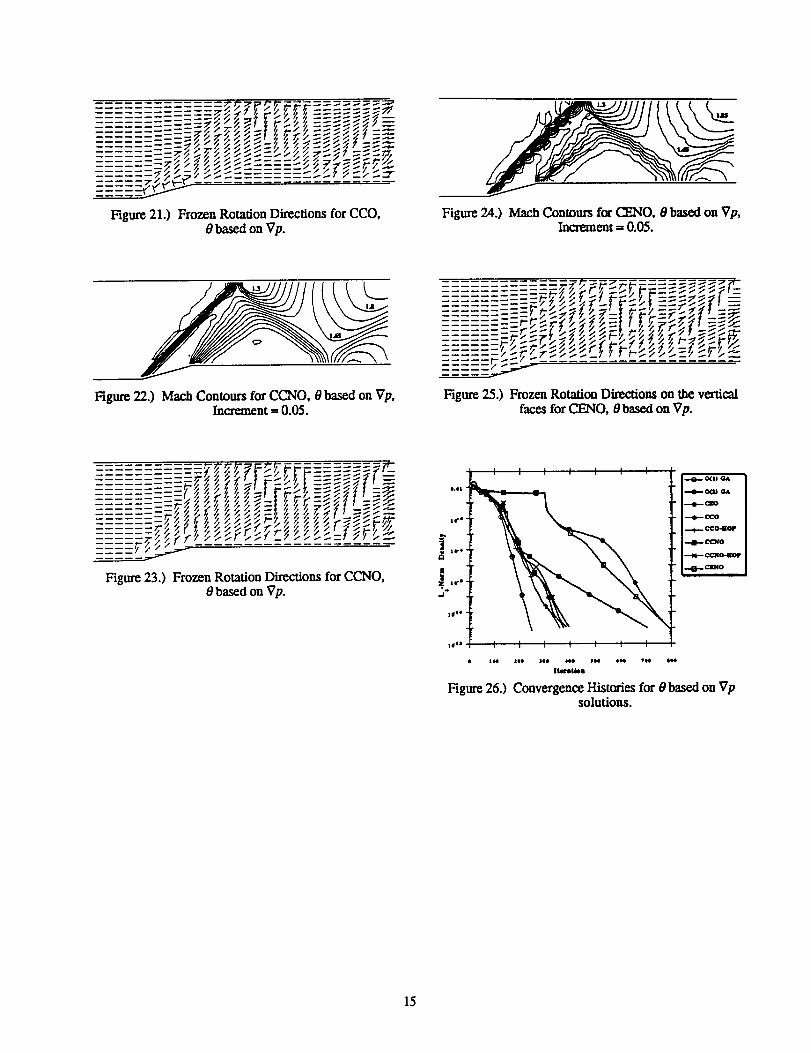
The next set of results is computed using the fourstrategies with the rotation angles based on the pressuregradient. The angles are computed every time step and thenfrozen at a particular level of convergence or maximumRer-_/on limit.

The CEO result is shown in Fig. 18. The solutionbased on pressure gradient does not show the signs of odd-even decoupling that were apparent in the 45 ° case.However, the solution is highly dispersive. The rotationangles are frozen after 300 iterations with a value ofDMIN=O.O0001. The frozen directions for the vertical facesare shown in Fig. 19 (every other line is plotted in thestreamwise direction while every llne is plotted in thecrossflow direction). While viewing Fig. 19, keep in mindthat an upwind flux is computed in both the preferred andnormal direction. The horizontal face directions are similarto those presented in Fig. 19. The horizontal vectors nextto the wall indicate that a grid aligned flux is computed.The directions are shown to basically align with the flowfield shock waves. However, around the initial shock wave,the angles are shown to be oscillatory. The oscillations inthe solution feed back to the rotation angle computation andcreate furtheroscillations in the solution. This effect can bereduced by filtering the rotation angle data as reported inRed'.[5].

The CCO results are presented next and are shown inFigs. 20 and 21. It is seen that the pressure gradient resultsare inferior to the 45 ° case but are still comparable to thesecond-order grid aligned solution. More precisely, theinitial shock wave is captured better but the improvementdiminishes as the shock waves are reflected clown thechannel. The rotation angles are frozen when the densityresidual reached a value of 5.x10 -4 and are shown in Fig.21. For this case DMIN---O.O005. The directions are shown

to align with the flow features and are well behaved. Recallthat the same angle computation algorithm is used in finiscase as in the previous CEO case. This is evidence that theill-hehaved directions of the CEO result are triggered by thecell-edge scheme. Again, no improvement is gained by themcae complicated projection.

The next set of results are for the CCNO method. The

Much contours are shown in Fig. 22. It is seen that theresults are similar to the CCO strategy although slightlymore dissipative. This is best seen in the fast reflectedshock wave. Also it is observed that the additionaldissipation, resulting from upwinding across the computedpressure gradient as opposed to setting the upwind directionto 45 °, triggers the spreading of the expansion fan therebyeliminating the expansion shock wave. The rotation angleswere frozen at the same convergence level as the previousCCO solution. A value of DMIN=O.O01 is used in

conjunction with Eq. [4.35]. The rotation directions are

mapped back into physical space and ate shown in Fig. 23.The directions are shown to vary smoothly. Once againthere is no improvement using the high_ order projection.

The lastcasecomputedistheCENO strategywiththerotationbasedon pressuregradient.The resultisshown inFig. 24. The solution is very similar to the CEO result ofFig. 18 although the non-orthogonal projection is slightlyless dispersive. The rotation angles were frozen after 300iterations and are shown in Fig. 25 (DM/N=0.001).

The convergence histories of the rotated solutions basedon pressure gradient are plotted in Fig. 26. The CFLnumbers and runtime data for the pressure gradient cases areshown inTable2. The followingobservationsaremade.First, the cell-edge schemes do not converge until therotation angles are frozen at 300 iterations. After thefreezing,theconvergencerateislessthanthecell-centerschemes.The cell-centerschemesconvergefaster than thesecond-ordergridalignedcaseand,interestinglyenough,takelessCPU timetocompute a comparablesolution.From experience,thecell-centerstrategieswillconvergeabout3 to3.5ordersofmagnitudebeforea limitcycleisreached.Freezingtheanglesallowscompleteconvergence.

Table2Code Performance Parameters,8 basedon Vp

CFL Iterations Time- gsec/pt-iterseconds

O(1) GA o, 248 2.00 6.72

0(2,) GA ,- 705 5.14 6.07CEO 3. 789 10.42 11.01CCO 20. 376 4.26 9.44CCO-HOP -- 360 4.33 I0.02CCNO 20. 389 4.04 8.65CCNO-HOP oo 399 4.58 9.57

CENO 7. 790 8.44 8.90

Throughout this study,the cell-edge schemes ate showntoconsistentlycream significant oscillationsinthesolutionof this channel problem. There have been a variety ofapproaches to reduce these oscillations. Levy computes the45 ° rotation case by only rotating the horizontal faces andcomputing a grid aligned flux on the vertical faces. Thiseliminates the oscillations but the improvement in shockcapturing ability is reduced. In the pressure gradient case,averaging of the rotation angles throughout the domain isemployed to reduce the feedback between the flow fieldoscillations and the rotation angle computation. Anothertechnique is the simplified interpolation scheme of Ref. [6].The simplified scheme reduces the dependence of tim flux onthe rotation angle since small changes in the angle do notchange the interpolated dependent states. The cell-centerstrategies, on the other hand, aBow greater flexibility in theangle selection and the interpolation. This is because theflux averaging, required in order to define a unique flux atthe face, acts as an inherent smoothing agent in the scheme.

lO

Fourrotatedupwindstrategieshavebeen tested on asimple Mach 2 channel flow problem It is concludedthecell-centerstrategiesofferbetterpromiseinextendingthestudytothreedimensionsthanthecell-edgestrategiesbecauseofthereductioninwork,theinherentsmoothinginthefluxaveraging,andacceptableconvergencerates.TheCCO strategyproduces the bestresultsof the four

strategies.The resultsarecomparabletothesecond-ordergridalignedscheme. The CCNO strategyalsoproducesgoodresults,issimplertoincorporatethanCCO, and hastheaddedfeatureofrevertingm agridalignedformulation.Finally,itisshown thatforthissimpletestcase,thehigherorderprojectiondoesnotimprovethecell-centerresults.

This researchis supportedby NASA Grant No.NAGW-1331 to the Mars Mission Research Center.

Additionalsupporthasbeenallocatedby theNASA-AmesResearchCenter,MoffetField,California,underInterchangeNo. NCA2-719. The authorswould alsoliketothankthe

North Carolina Supercomputing Center for the use of theirfacilities.

References

[1] Roe,P.L. (1981), "ApproximateRiemann Solvers,ParameterVectors,andDifferenceSchemes,"JournalofComputationalPhysics,Vol.43, 1983,pp.357-372.

[2] Rumsey, C.L., "Development of a Grid-IndependentApproximate Ricmann Solver," Ph.D. Dissertation,Department of Aerospace Engineering, University ofMichigan, 1991.

[3] vanLeer,B.,"ProgressinMulti-DimensionalUpwindDifferencing,"Proceedingsof the13thInternationalConference on Numerical Methods in Fluid

Mechanics,Rome, July 1992, LectureNotes in

Physics,414,Springer-Vcdag,pp.1-26.

[41Davis, S.F., "A Rotationally Biased Upwind DifferenceScheme for the Euler Equations," Journal ofComputational Physics, Vol. 56, pp. 65-92.

[5] Levy, D.W., Powell, K.G and van Leer, B., "AnImplementation of a Grid-Independent Upwind Schemefor the Elder Equations," AIAA Paper 89-1931-CP,1989.

[6] Dadone,A. and Grossman,B.,"A RotatedUpwindScheme fortheEulerEquations,"AIAA Paper91-0635,January,1991.

[7] Kontinos,D.A. and McRae, D.S.,"An Explicit,RotatedUpwind Algorithm for Solutionof theEuler/Navier-StokesEquations,"AIAA Paper 91-1531-CP,1991.

[8] Leek, C.L., and Tannchill, J.C., "A New RotatedUpwind Difference Scheme for the Euler Equations,"AIAA Paper 93-0066, January,1993.

[9] Levy, D.W., PoweU, K.G and van Leer, B., "Use of aRotated Riemann Solver for the Two-DimensionalEuler Equations," Journal of Computational Physics,Vol. 106, 1993, pp. 201-214.

[10] Yoon, S. and Jameson, A., "An LU-SSOR Schemefor the Eulcr and Navier-Stokes Equations," AIAAPaper 87-0600, Jan. 1987.

[11]Thompson, J.F., Warsi, Z.U.A, and Mastin, C.W.,"Numerical Grid Generation," Elsevier SciencePublishing Co., Inc., 1985, Chapter I]].

Y

• CellCenters

/ij+111/ e Inte o onPoints lru ..'

Hgure I.)Cell-EdgeOrthogonalFluxStrategy.

11

y i/

E2 _2 ij+l i+1j+1 If 0

X

__ " Ce.C,nter _ _,. CeHCent_

_, 7_r. i .._../J'X\ 0 Interp Point * Intcrp Point

4 a) Computational Spacen

Figure 2) Cell Cen_r Orthogonal Flux Strategy _tn

• Cell Center

I _ _ • InterpPoint

-.o 4 • CeU Center_3 b.)Physical Space

\, o Interp Point

_4 Figure 4.) CeU-EdgeNon-Orthogonal Flux Strategy.

a.) Computational Space

2 _ _2

n_ ; CeUCenterimerpPoint Figure5.)ProjectionVectors.

_3

_4

b.) Physical Space

Figure3.)Ceii-CenterNon-OrthogonalFluxStrategy.

12

7/

i+lj+l

_ i+lj

e Cell Cemer

Figure 6.) Cell-Edge Interpolation Stencil.

_'2 ij+ ll2

i-ll2J t i 'l _'l

F'3 _ V / i+l/2d

./I/ /,\/,j-1/2 _,

half plane F2 half plane

F3 half plane F4 half plane

Hgurc 7.)Hux ProjectionoverParallelogram

Hgum 8.)6Ix2I Grid

Hgurc 9.) Mach Contoursfor F'gst-Ordcr GridAligned, Increment = 0.05.

Figure 10.) Mach Contours for Second-Order GridAligned, Increment = 0.05.

Figure 11.) Mach Contours for CEO, 0=45%Increment = 0.1.

Hgurc 12.) Mach Contours for CEO, 6e45 °, Entropy Fix,Increment = 0.05.

13

Figure13.)Mach ContoursfoxCCO, _.45°,Increment= 0.05.

FigUl_ 14.) Mach Contours fox CCO, Higher OrderProjection, 0=45 °, Increment = 0.05.

Figure 15.) Maeh Contours for CCNO, 0=45°,Increment = 0.05.

Figure16.)Mach ContoursforCENO, 0--45°,EntropyFix,Increment= 0.05.

le'4

]te "_e

|

._ 1_ a

I I I I I I

o_l " .--.0.--o0) q_,

...4I--.OBO

..,4k... (_o

•.-4.-.. CCO-I_OlP

--.(B-- Cello

-..tl4_ O(_IO-EIOF

--,O--.¢lNO

|(i-I e

:o'" I I I I I I

e lee 404) ¢ee e(NI IINI4 tg_ I4N

|_rmUom

Figure 17.) Conv_gencc Histoxics for 0=45 ° Solutions.

Figure 18.) Mach Contours for CEO, 0based on Vp,Increment = 0.05.

, _..'_ _ _

:::::_-:::::=:_7:_-s-_-_-'<,_×,__,_ _!i_:,_A_/_":,3__....... /_ ,_xx _,,...... __ /_ ,xx _,

:: ::z _.._:_

Figure 19.) Frozen Rotation Directions on thevertical faces for CEO, Obased on Vp.

Figure20.)Mach ContoursforCCO, 0basedon Vp,Increment= 0.05.

14

........ _ × _ _ _./. -/1I "/."/,:,7 _ .../ × -,r._ _._

---_7/_ ..-_._ _ _ ....... :,.:_,= .... _._/:

.__ ,_._............. . ......

Ngur_ 21.)FrozenRotationDirectionsforCCO,0 basedon Vp.

Figuro 24.) Mach Contours for CENO, 0 based on Vp,Increment = 0.05.

Figure 22.) Ma_h Contours for CCNO, 0 based on Vp,Incrmnent = 0.05.

-_--- _=-_, ......... _.___ ,z'-,_'/_- _.---:'_ _-" _ _-_ _ _ _-_ F"-----.---'-'_ _ _- _._<! _. P. z_..=_'_------_ _._ • _ _"_=I_- _ _ _.--:_ _ _ - -'-

_ i--_- --_ .....................

Figure25.)FrozenRotationDirectionson thevertical

faceaforCENO, 0basedon Vp.

...... --ZX Z f' g Z Z/_;_P"7 Z ZX ZZ .-.//

.... _/.'/7f 7 __ 11,,...___1// _*_

Figure 23.) Frozen Rotation Directions for CCNO,0 basedon Vp.

I ! I I I I I

141-'1

!"i

Figure 26.) Convergence Histories for 0 based on Vpsolutions.

.-.+.. _o41o1_

15

AIAA 94-2291

Rotated Upwind Algorithms forSolution of the Two- and Three-Dimensional Euler and Navier-

Stokes Equations

D.A. Kontinos and D.S. McRaeNorth Carolina State University

Raleigh, NC

25th AIAA Fluid Dynamics" Conference

June 20-23, 1994/Colorado Springs, CO

For permission to copy or republish, contact the American Institute of Aeronautics and Astronautics370 L'Enfant Promenade, S.W., Washington, D.C. 20024

Two-

Rotated Upwind Algorithms for Solution of theand Three-Dimensional Euler and Navier-Stokes Equations

D.A. Kontinos* and D.S. McRaef

North Carolina State UniversityRaleigh, North Carolina

Abstract

Rotated upwind algorithms are presented for thenumerical solution of the Euler and Navier-Stokes

Equations in two and three dimensions. The finite-volumealgorithms axe designed with the notion of aligning Roe'sapproximate Reimann solver in a computed preferreddirection. The algorithms are applied to shock wavereflection and shock-wave/boundary-layer interaction

flowfields typically found in supersonic and hypersonic inletconfigurations. Calculation of an inviscid Math 2 channelflow problem shows that the rotated algorithm producesmore accurate results than a traditional grid aligned

algorithm to both first- and second-order accuracy.Moreover, the improvements to second-order accuracy are asgreat as those to first-order accuracy. Viscous solution of aturbulent boundary layer / shock wave impingement showthat the rotated scheme improves the shock wave capturingin the inviscid portion of the flowfield to both first- andsecond-order accuracy. The improvements in the shockwave capturing to first-order accuracy result in improvedwall pressure and skin friction distributions. However tosecond-order accuracy, the wall predictions are not improved.The calculation of an inviscid three-dimensional shock wave

surface shows the rotated algorithm to be more accurate than

the grid aligned algorithm to both first- and second- orderaccuracy. The accuracy improvements in three dimensionsare not as great as those in two dimensions. Computationof a viscous flowfield in the corner of two intersecting

wedges shows that the inviscid portions of the flowfield are

qualitatively improved with the rotated algorithm to bothfirst- and second-order accuracy. However, surface pressure

predictions are only marginally improved with the rotatedalgorithm.

Much of the recent algorithm development has beenfocused on creating artificial dissipation models that includemulti-dimensional effects. It is hoped that the great success

of the upwind dissipation models can be extended by moreaccurately modeling wave propagation in multi-dimensional

* Research Assistant, Mechanical and Aerospace

Engineering, Student Member AIAA.t Professor, Mechanical and Aerospace Engineering,Member AIAA.

Copyright © 1994 American Institute of Aeronautics andAstronautics, Inc. All rights reserved.

space. A variety of promising and novel approaches arecurrently being pursued. Since the number of methods hasbecome too numerous to list in this format, the reader isreferred to a comprehensive overview of the multi-

dimensional methods presented by van Leer 1.

One approach to including multi-dimensional effects inthe flux function is the use of a rotated upwind method.The idea, originating with formulations of the potential

equations 2.3 and later developed by Davis 4 for the Eulerequations, is to rotate the integration stencil to anorientation where the differencing is applied in a direction

that more closely models the correct path of informationpropagation. For the Euler and Navier-Stokes equations,rotation results in applying the upwind formulation acrosscaptured discontinuities rather than along grid lines. Theorientation of the upwind operator with respect to flow

discontinuities significantly impacts the ability of theupwind model to correctly interpret local wave propagation.

For example, Roe's 5 scheme is known to model a singleshock wave as a sum of acoustic and shear waves if the

operator is applied oblique to the shock wave (an excellentdiscussion of this effect is presented in Ref. [6]). Theadditional non-physical shear wave generates excess

dissipation and smears the captured shock wave. However,the correct wave propagation is predicted when the operatoris applied across the shock wave. Thus, we are motivatedto calculate an upwind flux across flow discontinuities

independent of the orientation of the discontinuity withrespect to the grid.

Many rotated upwind schemes for solution of the Eulerequations have been developed 7.g,9,10, all of which showincreased shock resolution as compared to traditional gridaligned schemes for simple inviscid test problems to first-order accuracy. The improvements to second-order accuracyare shown to be modest but encouraging. Furthermore,none of the previous rotated upwind schemes have beenextended to three dimensions. In fact, very few of the newly

developed multi-dimensional upwind methods have beentested in three dimensions. Some exceptions are the worksof Deconinck et. al.11 for three-dimensional scalar

advection, and Rumsey 6 who solves the Euler equations inthree dimensions. Rumsey's results show improvement ofthree-dimensional shock and shear capturing to f'trst-order

accuracy. To second-order accuracy, only improvement toshear capturing is shown. Thus, it has not beendemonstrated, nor is it necessarily anticipated, that a rotated

upwind scheme that aligns the Roe operator in a singlepreferred direction in three-dimensional space will improve

three-dimensionalshockwavecapturing.It is theobjectiveof this study to develop a robust, rotated upwind algorithmfor the solution of both the Euler and Navier-Stokes

equations in two and three dimensions. The necessarycharacteristics of this scheme are that it is fullyconservative, second-order accurate in space, and sufficientlyrobust to compute a variety of supersonic throughhypersonic flow fields.

2,0 The Navier-Stokes Equations

For this study, the governing equations are the set of

conservation laws governing three-dimensional viscous fluidflow known collectively as the Navier-Stokes equations.The equation set in integral form and in index notation isgiven as the following:

_--- ]pdV+ ](puini)dS=O, (2.1)03t Votu_ S_/ace

f pujdV ÷ f (puiuj + To )nidS = OOt

Volumt Surface

(2.2)

IPEtdV+ I(Etui+Tqu,+ql)nldS=O, (2.3)_t vot_ s_'lac,

where p is the density, ul is the velocity, Et is the total

energy, ni is the outward normal to the surface bounding

the control volume, qi is the heat flux, d V is the

differential element of the control volume, and dS is the

differential element of the bounding surface. The term T o

is the stress tensor which contains both the pressure andshear stress terms. The shear terms are modeled assuming alinear stress-strain relation, the heat flux is modeled throughFourier's law, and the dynamic viscosity is calculated usingSutherland's Law. In addition, the perfect gas equation ofstate is employed.

The governing equations are solved in a finite-volumeformulation with the conserved variables taken as averagesover the cell volume. The surface integrals of Eq. (2.1 -2.3) become summations over the cell sides. Expanding thevector momentum equation into its scalar components, theequations for a fixed grid become,

= ! Y:.S (2.:)Ot Volume _ '

where U is the vector of dependent, conserved variables and

P contains the fluxes. The cell face normal as expressed in

terms of the grid metrics is denoted by ._. The magnitude

of S is equal to the cell face area. The Euler equationsubset is obtained by neglecting shear terms.

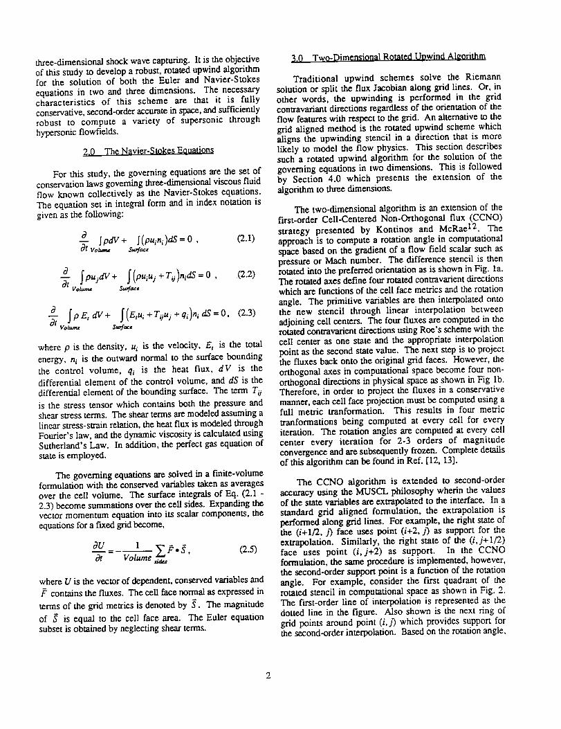
3,0 Two-Dimensional Rotated Upwind Algorithm

Traditional upwind schemes solve the Riemannsolution or split the flux Jacobian along grid lines. Or, inother words, the upwinding is performed in the gridcontravariant directions regardless of the orientation of theflow features with respect to the grid. An alternative to thegrid aligned method is the rotated upwind scheme whichaligns the upwinding stencil in a direction that is morelikely to model the flow physics. This section describessuch a rotated upwind algorithm for the solution of thegoverning equations in two dimensions. This is followedby Section 4.0 which presents the extension of thealgorithm to three dimensions.

The two-dimensional algorithm is an extension of thefirst-order Cell-Centered Non-Orthogonal flux (CCNO)strategy presented by Kontinos and McRae 12. The

approach is to compute a rotation angle in computationalspace based on the gradient of a flow field scalar such aspressure or Mach number. The difference stencil is thenrotated into the preferred orientation as is shown in Fig. la.The rotated axes define four rotated contravarient directions

which are functions of the cell face metrics and the rotation

angle. The primitive variables are then interpolated ontothe new stencil through linear interpolation betweenadjoining cell centers. The four fluxes are computed in therotated contravarient directions using Roe's scheme with thecell center as one state and the appropriate interpolationpoint as the second state value. The next step is to projectthe fluxes back onto the original grid faces. However, theorthogonal axes in computational space become four non-orthogonal directions in physical space as shown in Fig lb.Therefore, in order to project the fluxes in a conservativemanner, each cell face projection must be computed using afull metric tranformation. This results in four metric

tranformations being computed at every cell for everyiteration. The rotation angles are computed at every cellcenter every iteration for 2-3 orders of magnitudeconvergence and are subsequently frozen. Complete detailsof this algorithm can be found in ReL [12, 13].

The CCNO algorithm is extended to second-orderaccuracy using the MUSCL philosophy wherin the valuesof the state variables are extrapolated to the interface. In astandard grid aligned formulation, the extrapolation isperformed along grid lines. For example, the right state ofthe (i+1/2, j) face uses point (i+2, j) as support for theextrapolation. Similarly, the right state of the (i,j+l/2)face uses point (i, j+2) as support. In the CCNOformulation, the same procedure is implemented, however,the second-order support point is a function of the rotationangle. For example, consider the first quadrant of therotated stencil in computational space as shown in Fig. 2.The gust-order line of interpolation is represented as thedotted line in the figure. Also shown is the next ring ofgrid points around point (i,j) which provides support forthe second-order interpolation. Based on the rotation angle,

one could follow the same liner interpolation procedures asthe f_rst-order stencil. However, the second-order supportring consists of six points thus requiting logic to determinethe location of the interpolation. Such a procedure

significantly increases the amount of work required by thealgorithm. An alternative procedure is implemented in thisstudy. The second-order support point is taken to be theclosest cell center value to the intersection of the rotated

axis with the second-order support ring. Thus, the second-order interpolation is not a continuous function of therotation angle, but is a step function. Of course, theintroduction of a discontinuous interpolating function

dictates that the rotation angles must be frozen in order toreach convergence. If the angles are not frozen, it is veryprobable that the second order interpolation will cyclebetween two discontinuous values. But since it is seen in

Ref. [12] that the rotation angles are frozen in order to

converge the first-order algorithm, the discontinuous second-order interpolating function does not introduce any furtherlimitations.

The final component of the flux computation of theCCNO algorithm are rotated boundary conditions. Sincethe rotation angles are defined at the cell centers, the fluxcomputation of each of the four faces surrounding aparticular cell center are essentially coupled. Consequently,reflection and extrapolation boundary procedures commonly

employed in grid aligned schemes must be modified toaccount for the coupling of the boundary faces withadjoining interior faces. The details of the boundarycondition procedures are omitted here for brevity but arepresented in Ref. [13]. Finally, the viscous fluxes arecomputed in the standard grid aligned fashion and thesolution is relaxed in time using the diagonal form of theLU-SGS scheme of Yoon and Jameson 14.

4.0 Three-Dimensional Rotated Upwind Algorithm

This section will outline the development of the three-dimensional cell-centered non-orthogonal flux rotatedupwind scheme. Recall, that the overall strategy of theCCNO scheme is to compute a preferred upwind direction incomputational space at each cell center. Then a coordinaterotation is performed such that a computational axis isaligned in the preferred direction. Primitive variables arethen interpolated onto the new coordinate system. Theinviscid fluxes are computed and transformed back onto thegrid faces in a conservative manner. Sections 4.1-4.4 detailthe steps of the algorithm. Section 4.1 presents thecoordinate rotation that aligns a coordinate axis with anyarbitrary direction. The rotation matrix defined in Section4.1 is then used in Section 4.2 to define the contravariant

directions of the rotated fluxes. Section 4.3 presents theinterpolation procedure and Section 4.4 describes theprojection of the rotated fluxes onto the original grid faces.

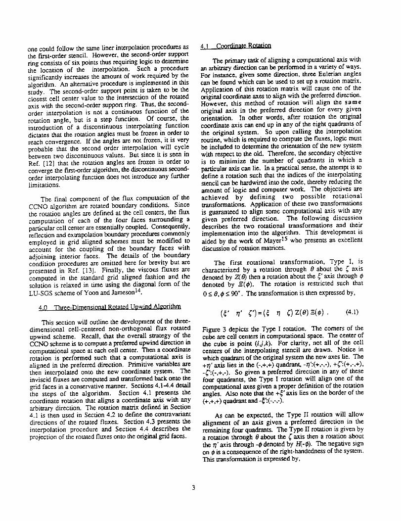
4,1 Coordinate Rotation

The primary task of aligning a computational axis withan arbitrary direction can be performed in a variety of ways.For instance, given some direction, three Eulerian anglescan be found which can be used to set up a rotation matrix.Application of this rotation matrix will cause one of theoriginal coordinate axes to align with the preferred direction.However, this method of rotation will align the sameoriginal axis in the preferred direction for every givenorientation. In other words, after rotation the originalcoordinate axis can end up in any of the eight quadrants of

the original system. So upon calling the interpolationroutine, which is required to compute the fluxes, logic mustbe included to determine the orientation of the new systemwith respect to the old. Therefore, the secondary objectiveis to minimize the number of quadrants in which a

particular axis can lie. In a practical sense, the attempt is todefine a rotation such that the indices of the interpolatingstencil can be hardwired into the code, thereby reducing theamount of logic and computer work. The objectives areachieved by defining two possible rotationaltransformations. Application of these two transformations

is guaranteed to align some computational axis with anygiven preferred direction. The following discussiondescribes the two rotational transformations and their

implementation into the algorithm. This development isaided by the work of Mayer 15 who presents an excellentdiscussion of rotation matrices.

The first rotational transformation, Type I, ischaracterized by a rotation through 0 about the _ axisdenoted by Z(g) then a rotation about the _' axis through 0denoted by _($). The rotation is restricted such that

0 < 0, $ < 90*. The transformation is then expressed by,

n' n (4.1)

Figure 3 depicts the Type I rotation. The corners of thecube are cell centers in computational space. The center ofthe cube is point (ij,k). For clarity, not all of the cellcenters of the interpolating stencil are drawn. Notice inwhich quadrant of the original system the new axes lie. The+r/' axis lies in the (-,+,+) quadrant, -r/':(+,-,-), +_":(+,-,+),-_":(-,+,-). So given a preferred direction in any of thesefour quadrants, the Type I rotation will align one of thecomputational axes given a proper def'mition of the rotationangles. Also note that the +_' axis lies on the border of the(+,+,+) quadrant and -_':(-,-,-).

As can be expected, the Type II rotation will allowalignment of an axis given a preferred direction in theremaining four quadrants. The Type II rotation is given bya rotation through 0 about the _"axis then a rotation aboutthe r/' axis through -0 denoted by/-/(-_). The negative signon ¢Jis a consequence of the right-handedness of the system.This transformation is expressed by,

(_" ,7" ¢')=(_ n ()z(o)H(-,). (4.2)

Figure 4 depicts the Type II rotation. Now it is seen thatthe +_' axis lies in the (+,+,+) quadrant, -_':(-,-,-),+_:(+,-,-), -(':(-,+,+). The +r/' axis lies on the border of the(-,+,+) quadrant and -r/':(+,-,-). Comparing Type I and TypeII rotations it is seen that the ends of _' and r/' always lie inthe same quadrant. Thus, for the _' and 77' axes the

objective of minimizing the number of possibleorientations has been achieved. It is only (' which requiressome logic to determine indices of the interpolating stencil.However, each end of the (" axis can only lie in one of two

quadrants. Superposition of the two transformations resultin the following rotation matrix,

cos(o)(p +gcos(_)) _sin(_)

- sin(¢,)(,:_cos(O)+/3sin(o)) cos(cO

(4.3)

where is _z = 1 for a Type I rotation, g = 0 for a Type IIrotation, and/3 = 1-tz.

To completely define the rotation, the angles and theswitch between Type I and Type II rotation must becomputed. First let the preferred direction in computational

space be given by _,i,_f=(p_+q_+r_) where the ^

denotes some unit normal in computational space. Theswitch between types of rotations is given as,

for pq _ 0

(4.4)

Before computing the rotation angles, the orientation of thepreferred direction is revealed by computing the followingswitch functions,

i for pq _ 0(_ pq =

for pq < 0

(4.5)

Ifor qr_>06¢, = , (4.6)

0for qr < O

i for pr >_0¢_pr =

for pr <0

(4.7)

_" = aSq, +/_Sp,. (4.8)

Then from geometric considerations the angles are given by,

cos(O) = _,_IP[+ (1- 3eq)lq[p2 + q2

(4.9)

cos(_,)(1- d:)lr[+ 8" P'_ q2= (4.10)p2 + q2 + r 2

The complete range of rotation is 0 < 0,¢_ < 90 ° so that thecosine of the angles is sufficient.

4.2 Contravariant Directions

The rotation matrix developed in the previous section isused to define the contravariant directions of the new

coordinate system. Recall that the advantage of defining therotation in computational space is that the scheme willautomatically revert to a grid aligned formulation.Moreover, the scheme reverts to a grid aligned mode in thelimit of 90 ° rotation. Conceptually, the coordinatetransformation rotates each coordinate axis between

adjoining cell face normals which are the contravariantdirections of the grid. For example, let J be the metric

Jacobian matrix given by,

r/,J = _ 77y (4.11)

In a finite-difference formulation, the metrics are defined at

the grid point so that the metrics of a new coordinatesystem, denoted by J" are unambiguously given by,

J'= R(a, O,¢,)J. (4.12)

In a finite-volume formulation, the metrics are def'med at the

cell face. Therefore, under a cell centered coordinaterotation, the new metric Jacobian is not clearly defined.

However, the rotation matrix does prescribe the propertransition between the cell face normals under a rotation in

computational space. Consider the +4" rotated contravariantdirection as an example. We know that under the given

rotation,the+_' axisalwaysliesin thefin'st quadrant ofcomputational space. Furthermore from observing thelimits of 0° or 90 ° rotation of both 0 and ¢, it is apparentthat the contravariant direction is some function of the

metrics of faces (i+1/2, j, k), (i,j+l/2, k), and (i,j, k+I/2).Therefore the transformation of the +_' axis is given by,

j" = R(a, 0, ¢) •

Lc:<,,,,,¢,<,>.,,,

(4.13)

It is important to note that this transformation yields thedirection of the +_' axis only, consequently, only the toprow of elements of J' is needed giving,

_ = sTti+ J6J + jfik , (4.14)

where j,_ are the elements ofJ'and _l is the contravariant

direction of the +_' coordinate axis.

The other five contravariant directions are defined bydeveloping some simplifying notation. First, let J(a,b,c) bedefined as follows,

J(a,b,c)= I r7_t.._ rly_,+,,+

_ I i÷,,,,ti,l

r/, j+,, (4.15)

_Zl, j,,t*c

Here, a, b, and c assume values of _+1/2 to select the sidesof the computational cube at point (i, j, k). Furthermore,let the function ROW(m, A) give the vector on the ruth

row of matrix A. Then the fit direction developedpreviously is denoted as

,_' = ROW(I, R(a,O,O)J(i/2,it2,,/2)) (4.16)

The remaining conlxavariant directions are developed in asimilar manner and are given as,

fi2 =ROW(2, R(a,O,¢)J(-ll2,1/z,,12)), (4.17)

fi3 = ROW(l, R(ct, O,_)J(-i/2,-,12,-,/2)) , (4.18)

-a ROW(2, R(a,O,O) J(t/2,-ll2,-t/2)) , (4.19)/l =

_5 = ROW(3, R(_X, 0, ¢_)J(a -i/2,-,/2,1/2)) , (4.20)

ffs= ROW(3, R(a, O,0) J('/2- O/,i/z,-I :2)) , (4.21)

where _2, ,_3, _4, _s, and _6 al_ the contravariant

directions of the -_', +7/', 47', +_", and -_' axes, respectively.

4,3 Interoolation

Once the rotation of Section 4.1 has been defined, the

interpolation of the primitive variables can be performed.In fact, one of the advantages of rotating in computationalspace is that there is symmetry of the interpolation stencilabout the cell center. The first-order interpolation isperformed by computing eoorclinates of the interpolating rayand then using a trilinear interpolating function over a

quadrant of computational space. For example, consider the

(+,+,+) quadrant of Fig. 5 where the fit ray is shown undera Type II rotation. Let the origin of (_, r}, _ be at point

(i, j, k). Then over the region of the cube any value 0 can

be given by the trilinear function,

0 = (1- ¢)[ ¢qi+1,73: + 17qi.)+l.a -(1- ¢ )(1- rl)qi.j.a

+_rl(qi+l.j+i.,-qi+i.,.t- qi.)+l.t)] (4.22)

+_[ _qi+,..i.,+i + rTqi.)+,.t+, -(1- ¢)(1- rl)qi.j.l,+ ,

+_rl(qi+,.,+,.,+,- qi+l.j.,+!.-qi.)+,.#++,)].

All that needs to be deemed are the coordinates (_,rl,O in the

range 0 < _, 77,_"< 1. Of course it is desirable to define the

coordinates such that for no rotation, a grid aligned schemeis recovered. One possible option is to set (_,r/,_) such that

,_2+ 712+ _2 = 1. This is shown as the shell segment

drawn in Fig. 5. This is the easiest option to implementbecause all that is required is a normalization of the

coordinates defining the interpolating ray. The option usedin this study is to clip (_,r/,g") where the interpolating rayintersects the outer face of the interpolating stencil. Then

the trilinear function of Eq. (4.22) in effect reduces tobilinear interpolation over the outer square region.Moreover, if the interpolating ray happens to intersect theline segment adjoining two grid points, the interpolatingfunction reduces to linear interpolation. This second optionis selected so that under/overshoots are minimized through alow order interpolating function. Similar expressions toEq. (4.22) are written for the other quadrants of theinterpolating stencil.

The second-order interpolation of the three-dimensionalalgorithm is similar to the two-dimensional procedure of

Section3. Thesecond-orderinterpolantvalue is taken asthe nearest cell center value to the interpolating ray.

Consider the first quadrant of the second-order stencil asshown in Fig. 6. In the first quadrant, there are 19 pointsin the stencil which are displayed in Fig. 6 as black and

gray circles (excluding (i, j, k)). The discontinuousinterpolation function must be able to select the nearest cellcenter value to the interpolating ray. Such a function iscostly because there are 19 possible interpolant values.Consequently, the stencil is reduced to be composed of the 7comer points which are shaded black in Fig. 6. The indicesof the nearest cell centers are calculated based on thecoordinates of the first-order interpolating ray. Details of

this procedure are contained in Ref [13].

4,4 proiection

The inviscid fluxes are computed using Roe's schemewith the cell center point as one state, the appropriateinterpolated point for the second state, and the rotatedmetrics defined in Section 4.2. At this point in the

computation, there are six fluxes computed in the rotatedcontravariant directions. In order to maintain conservation,

the fluxes must be projected back onto the original gridfaces. Recall that the fluxes are orthogonal incomputational space; however, they are non-orthogonal inphysical space. Therefore, in order to project the fluxes, anew transformation must be computed for each face basedon the contravariant directions as is done in the two-

dimensional algorithm. The three-dimensionaltransformation can be found in Thompson et. al.16. Once

again for emphasis, the full transformation must becomputed at each grid point for each face in order tomaintain conservation. This results in six metric

transformations being computed at each grid point everyiteration. Unfortunately, this requirement causes significantincreases in the algorithm's work load.

The projection schedule for each of the six faces of thecell is now given. Three fluxes are required per face and areselected such that in the limit of 90* rotation the

contravariant directions are properly oriented in a grid

aligned fashion. For example, the to/• Si+l/2d,k flux (where

fit is the inviscid flux and Si+tt_,j._ is the cell face normal

of face (i+1/2, j, k)) must be a function of the contravariantdirections thnr have a (i+1/2, j, k) metric dependency. From

Eq. (4.16) and Eqs, (4.19 - 4.21) it is seen that _1, h_ ' _s,

and E6 all have a (i+1/2, j, k) metric dependency. Letting

H represent the transformation, the projection dependencyfor face (i+l/2,j, k) is given by,

to,• = (4.23)

where F_=ff/*_ " and a and fl are the switching

coefficients between Type I and Type II rotation. Theprojection schedule for the remaining faces are given as,

tOt ",_i-,,2.).k = H(F2.F3,_FS,aF'), (4.24)

ff', "S-i.)+u2.k = H(F1,FZ. F6) , (4.25)

tOt" S-i.j-l/2.k = H(F3,F4,FS) , (4.26)

F, " S-'i.).k+l/2 = H(F1,FZ,FS) , (4.27)

Ft " Si.i.k_ll 2 = H(F3,F4,F') . (4.28)

The two numerical flux values from each adjoining cellcenter rotation around a particular face are averaged in orderto uniquely define the cell face flux. Also, rotated boundaryconditions are implemented in three dimensions and aredescribed in Ref. [13].

5.0 Results

5.1 Inviscid. Much 2. Channel Flow

The two-dimensional CCNO algorithm is tested by

computing a Much 2 flowfield in a channel with a 15° rampwhich can be found in Ref. [7]. This geometry has beenused quite extensively as a test case for multi-dimensional

upwind algorithms. The deceptively simple geometry

belies the intricate physics of the flow. In fact, fine ,g)'idresolution studies of this case by Parpia and Parikh 17 show

that the initial shock wave does not reflect in a regularmanner off of the top wall. Instead, a Much stem developsand a slip surface is generated at a triple point. These flowcharacteristics are not captured with the 61x21 grid (Fig. 7)used in this study. The case is computed using the standardgrid aligned upwind formulation and the resulting Muchcontours are shown in Fig. 8. The contours range from 1.3to 2.0 in increments of 0.05. The case is computed usingthe CCNO algorithm to ftrst-order accuracy. The preferredupwind direction is selected to be the direction of thepressure gradient. The resulting Mach contours are shownin Fig. 9. The rotation angles are computed for every cellevery iteration until the L2-Norm of the mass equation is

reduced by approximately three orders of magnitudewhereupon the rotation angles are frozen. The freezingoccurs in 260 iterations and the resulting orientations areshown in Fig. 10. The solution converges 12 orders ofmagnitude in 453 iterations at a CFL of 5 consuming 2.9seconds of Cray Y-MP/C90 time.

The first-order CCNO method is shown to capture theshock waves with less smearing than the first-order gridaligned result of Fig. 8. The solution is relativelyoscillation free except for a leading overshoot ahead of the

rampshockwave.A pressuresurveythroughthemiddleofthe domain is shown in Fig. 11. The pressure comparisonclearly shows that the rotated scheme captures thediscontinuities and associated pressure rises more sharplythan the grid aligned procedure to first-order accuracy. Inorder to quantify the error, a fine grid solution of 385x129

points is computed using the second-order grid alignedscheme. This solution is considered to be the "exact"solution of an error norm calculation. Mach number

contours of the 385x129 grid solutions are shown in Fig.12. Based on the fine grid solution, the density L2-error-

norm of the f'trst-order grid aligned solution is calculated tobe 4.561x10 -3 while the first-order CCNO error is

2.521x10 -3. Analysis of the error distribution reveals that

the major source of error is the smearing of the capturedshock waves.

The increase in accuracy of a first-order rotated schemehas been shown by previous researchers e.g. Levy et. al.7,Dadone and Grossman 8, and Kontinos and McRae 9,12.

However, the improvements of second-order accurate rotatedschemes over second-order accurate grid aligned schemeshave been shown to be modest at best. Thus, the CCNO

algorithm is now compared to grid aligned upwinding tosecond-order accuracy on the 61x21 grid. The Machcontours of the second-order grid aligned and CCNOsolutions are shown in Fig. 13 and 14, respectively. The

range and increment of the contours are the same as theprevious figures for direct comparison. The frozen rotationangles, based on the pressure gradient, are similar to thosein the first-order solution as shown in Fig 10. Fromcomparison to the second-order grid aligned result, it is seenthat the rotated solution shows improved shock wavecapturing. The improvement in the solution is alsoindicated in the pressure survey along j = 10 shown in Fig.15. The density error norm of the grid aligned and CCNOsolution are calculated to be 2.640x10 "3 and 1.345x10 -3,

respectively. Two very important observations can be madefrom the error calculation. First, the first-order CCNO

solution is more accurate than the second-order grid alignedresult. Secondly, and most importantly, the ratio of theerror norms show that the improvement of the CCNOsolution over the grid aligned solution is as great to second-order accuracy than to first-order accuracy. The CCNOsolution with CFL=5 converges 12 orders of magnitude in897 iterations in 7.33 seconds on the Cray Y-MP/C90.

The density error norms are plotted versus the numberof points in the x direction on a log-log scale in Fig. 16.Additional data points, generated from 97x33 and 121x41grids, are also included in Fig. 16. The figure shows thatthe rotated results are more accurate than the grid alignedresults to both first- and second-order accuracy.Furthermore, the improvements to second-order accuracy areas great as to first-order accuracy. It is also seen that theaccuracy gains are maintained as the grid is refined. Alsoshown in Fig. 16 are the slopes of the error lines whichindicate the numerical order of accuracy of the schemes for

this particular geometry. Of course the grid is not uniformin the y direction so the accuracy calculation based on the xdirection spacing is only approximate.

5,2 Turbulent Shock Wave Impingement

The next two-dimensional test case is a shock wave

impinging on an equilibrium turbulent boundary layer. Thecase is studied experimentally by Recta and Murphy 18 and isshown schematically in Fig. 17. A shock generator isinclined 13 ° to the incoming Mach 2.9 freestream. The

Reynolds number is 5.73x105 per cm, the temperature is

108 ° K, and the incoming boundary layer height is 1.694cm. The wall is measured to have a temperature of 291 ° K.At these conditions, the impinging shock wave creates an

adverse pressure gradient sufficient to separate the turbulentboundary layer. The separation region appears as anincrease in the thickness of the boundary layer and a shockwave is formed off of its leading edge. The flow thenexpands around the separation region and a second shockwave is formed at reattachment. Also shown in Fig. 17 isthe location of the theoretical inviscid shock wave

impingement location denoted by xi. The results are

presented with xi as a reference point. This flowfield is

measured by Recta and Murphy with two differentexperimental setups. In the first set-up, designated by G 1,the shock generator spans the width of the channel therebyencompassing the sidewall boundary layers. The secondsetup, designated by G2, includes side plates to remove theeffect of the sidewall boundary layers in order to isolate theshock-boundary layer interaction. It is found that includingside plates reduces the streamwise scale of the interaction

and lowers the pressure level of incipient separation. Theflowfields of both setups are inherently three-dimensional innature. It is found that as the shock generator angle isincreased, separation occurs at the comers of theconfiguration and spreads symmetrically toward thecenterline. At a shock generator angle of 13 °, the flow isseparated across the channel and a nearly uniform pressuredistribution is measured. However, the uniformity of thepressure distribution across the span is not a sufficientcondition for two-dimensionality of the flowfield.Consequently, comparisons of computed two-dimensionalresults to the experimental data must be made with caution.

The flowfield is computed using a 101x81 grid. Thepoints are equally spaced in the streamwise direction and aregeometrically stretched away from the wall. The minimum

wall spacing is near y÷ -- 1. The turbulence is simulated

using the one-equation turbulence model of Edwards and

McRae 19. The first-order grid aligned and CCNO pressure

contours are shown in Figs. 18 and 19, respectively. Thegrid aligned pressure contours show a smeared incident andreflected shock wave. The interaction region does not

indicate separation of the boundary layer. The CCNOpressure contours show the shock waves to be captured withless smearing. Furthermore, the pressure contours indicate

aninteractionregiontypicalof separatedflowsi.e.bothaseparationandreattachmentshockwavearevisible. Acomparisonof theskinfrictionalongthewallisplottedinFig.20. Alsoshownaretheexperimentallymeasuredseparationandreattachmentlocations.Theskinfrictionresultsverifythatthegridalignedsolutiondoesnotpredicta separationandthattheCCNOsolutiondoespredictaseparation.DespitetheCCNOscheme'spredictionof theseparationzone,bothsolutionsproducesimilarpressuredistributionsthatarenotin favorableagreementwiththeexperimentaldataasshowninFig,21. Theinitiationofthepressuresriseisnotpredictedwellandtheshapeofthedistributionisonlyinqualitativeagreement.Althoughthepressuredistributionsof thetwofirst-ordersolutionsareverysimilar,clearly the CCNO scheme more accuratelypredicts the character of the flowfield. The shock waves arecaptured with less smearing and the separation zone ismsrt_tre_

The grid aligned solution is run for 5,000 iterations at aCFL of 5,000 consuming 4.04 minutes of CPU on theCray Y-MP/C90. The CCNO solution is computed withthe rotation directions based on the pressure gradient. Therotation angles are damped to zero below the sonic line. Itis found that rotating the stencil below the sonic line in theseparation zone severely inhibits convergence. The solutionis first computed in grid aligned mode for 1,000 iterations ata CFL of 5,000 to allow the incident shock wave to set up.The rotation angles are then computed at a CFL of 50 up toiteration 9,000 upon which the angles are frozen. The CFLis then reduced to 5 and the solution is computed toiteration 16,000. The total CPU time is 15.73 minutes on

the Cray Y-MP/C90.

The shock impingement case is computed to second-order accuracy. The grid aligned pressure contours areshown in Fig. 22 while the CCNO pressure contours areshown in Fig. 23. It appears that the CCNO solution iscapturing the incident and reflected shock waves with greaterclarity. However, examination of the skin frictiondistribution of Fig. 24 reveals the two solutions predictvery similar results. Both second-order solutions overpredict the size of the separation zone. The pressuredistributions through the interaction zone are shown in Fig.25. The two schemes produce similar predictions which arein good agreement with the G1 data at the initial pressurerise. The post interaction pressure levels are in goodagreement with the experimental data as well. It is difficultto determine which of the two experimental data sets arebest used for a two-dimensional comparison. It is theintention of the experiment to reduce the three-dimensionality of the flowfield by cutting off the fullydeveloped turbulent sidewall boundary layers with the sideplates. Therefore, one anticipates that the G2 data is bestfor a two-dimensional comparison. However, adding theside plates generates laminar sidewall boundary layers thatare more prone to separation than their turbulentcounterparts. Thus, it is unclear which set of data is best to

compare against the computational results. Moreover, theeffectiveness of the turbulence model on this shock-

impingement case is uncertain. Regardless of thecomparison to the experimental data, it is important todiscover that the CCNO solution does not significantly alterthe flowfield predictions to second-order accuracy. The

pressure contours suggest that the CCNO algorithm yields aqualitatively better solution in the inviscid region of theflowfield, yet the wall predictions are quite similar.

The second-order grid aligned scheme is run for 19,000iterations consuming 15.31 minutes of CPU on the CrayY-MP/C90. The CCNO solution is computed with thesame rotation angle calculation as the first-order solution.The computation is run for 16,500 iterations in 19.07minutes. The rotation angles are frozen at iteration 10,000and are shown in Fig. 26.

5.3 Inviscid. Mach 2.8. Channel Flow

The first three-dimensional test case is Mach 2.8

inviscid flow in a four wall channel containing a ramp.

This test case is taken from Rumsey 6 and the geometry isshown in Fig. 27. The foot of the ramp is at an obliqueangle to the oncoming freestream and the inclination of theramp varies across the domain. The side boundaries are allsolid walls. With an inflow Mach number of 2.8, a trulythree-dimensional shock surface develops within the channelthus providing a challenging test of the three-dimensionalrotated scheme.

The case is run on a coarse grid with 41 points in thestreamwise direction and crossflow planes of 17x17. Allgrid points are evenly spaced along boundary line segments.The interior points are linearly interpolated between

opposite faces. One selected plane of the grid in eachcoordinate direction is shown in Fig. 28. The solution iscomputed to first-order accuracy with the grid alignedalgorithm. The resulting Mach number contours on threeselected planes interior to the domain are shown in Fig. 29.The contours for this and all subsequent contour plots rangefrom 1.4 to 2.8 in increments of 0.05. The predominantfeature is the ramp shock wave that reflects off of the topwall and exits the domain as shown in the j plane view.The k and i planes show variations across the domaindemonstrating the three-dimensional nature of the solution.

However, the In'st-order grid aligned results are highlysmeared and secondary flow features are difficult to discern.

The solution is computed using the three-dimensionalCCNO algorithm with the pressure gradient selected as thepreferred direction. The resulting Maeh contours are shownin Fig. 30. Clearly, the shock system is captured with lesssmearing using the CCNO algorithm. Not only is theprimary shock resolved to a higher degree, but secondaryshock structures that are smeared out with the grid alignedscheme are now evident. For example, the k plane view inFig. 30 shows a secondary shock wave emanating from a

triplepointmidwayacrosstherampshockwave.Thisfeatureis completelysmearedout in thegrid alignedsolution.

Thef'trst-orderresultsof theCCNO algorithm are

encouraging. Recall that few multi-dimensional upwindschemes have been developed and tested in three dimensions.Although certainly it can be predicted that aligning the Roesolver across a planar shock surface in three dimensions willreduce dissipation, it is not certain that any improvement atall can be expected by aligning a single coordinate axis in apreferred direction when crossing oblique shock waves existsuch as in this test case. Thus, the first-order results

present promise for the three-dimensional algorithm.

In order to quantify the error, a fine grid solution is

computed and considered as the "exact" solution of an errornorm calculation. The fine grid mesh spacing is one fourththat of the 41x17x17 grid thus yielding a 161x65x65 grid.The solution is computed to second-order accuracy with thegrid aligned scheme. The resulting Mach contours areshown in Fig. 31. Evident in the fine grid solution is thecurvature of the shock waves in the i and k planes as aresult of the increase in shock strength created by theincrease in ramp inclination across the domain. Moreover,the shock wave reflection off of the side walls creates a

triple point evident in both the i and k views. Acomparison of the first-order solutions to the fine gridsolution is provided in Fig. 32 where a pressure surveythrough the center of the domain in the streamwise directionis shown. The pressure survey demonstrates the improvedshock capturing ability of the CCNO algorithm.

The L2-norm of the mass equation of the first-order grid

aligned solution based on the fine grid solution is computedto be 1.889x10 3. The first-order CCNO error is calculated

to be 1.1314x10 -3. The ratio of the grid aligned to rotatederror is 1.670. Recall that in the two-dimensional inviscid

channel flow problem the error ratio is nearly 2. This is anindication that the improvement between grid aligned androtated schemes is greater in two dimensions than in threedimensions to first-order accuracy.

The solution on the coarse grid is computed to second-order accuracy. The grid aligned Mach contours are shownin Fig. 33 while the CCNO Mach contours are shown inFig. 34. From comparison between these two figures, it isseen that the rotated scheme improves the three-dimensionalshock capturing. The CCNO result shows the triple pointin the i and k planes while the grid aligned scheme onlyhints at its existence. Furthermore, a pressure surveythrough the middle of the domain, as shown in Fig. 35,also indicates improved accuracy. The mass equation errornorm (based on the fine grid solution) of the second-ordergrid aligned scheme is calculated to be 9.566x10 -'t while theCCNO error is 7.339x10 -4. The ratio of the error norms is

1.30. The improvements of the second-order accurate three-dimensional scheme are not as marked as the first-order

results. However, this is still an encouraging result. Themulti-dimensional wave model of Rumsey 6 showed no

improvements to second-order accuracy. Furthermore, keepin mind that only a single preferred direction is defined andthat the rotation is complete when a coordinate axis isaligned in that direction. There exists an additional degreeof freedom in the plane normal to the preferred directionwhere an additional rotation can be defined. Then one of the

two remaining coordinate axes could be aligned in somesecondary direction. In this current formulation, this optionis not explored and thus additional improvements may bepossible.

The convergence histories of the coarse grid solutionsare presented in Fig. 36. The first-order grid alignedsolution is run at a CFL of 10,000 and reaches a

convergence level of 10 -11 in 170 iterations and 11.4

seconds on the Cray Y-MP/C90. The second-order gridaligned solution is also run with a CFL of I0,000 andreaches convergence in 369 iterations taking 23.8 seconds.The CCNO solutions are both run at a CFL of 10 with the

preferred direction aligned with the pressure gradient. Forthe first-order CCNO solution the angles are frozen when

the residual reaches 9.x10 "4. Convergence is reached in 297iterations and 41 seconds of CPU. The second-order CCNO

rotation angles are frozen after 150 iterations. Convergenceis achieved in 593 iterations and 107 seconds.

Consistent with the two-dimensional inviscid results, itis seen that the CCNO algorithm takes longer to convergethan the grid aligned scheme. This is a result of thedecrease in numerical dissipation and a poor temporallinearizaton of the rotated fluxes. Recall that the implicitside does not account for the rotation of the fluxes. It is

also seen that the CCNO algorithm is significantly morecomputationally expensive than the grid aligned scheme.The grid aligned scheme (both first- and second-order) arerunning at approximately 6.3 micro-seconds per point periteration. The f'trst- and second-order CCNO algorithms arerunning at 13.5 and 17.6 micro-seconds per point periteration, respectively. A large portion of the increase isdue to the second-order interpolation because thecomputation of the interpolation indices does not optimizewell on the Cray Y-MP/C90. The other intensivecomputation is the three-dimensional transformation of therotated fluxes. An option to reduce this computation is tostore the results of the transformation after the angles havebeen frozen. The storage requirements are an additional 18real numbers per point. Furthermore, the indices of thesecond-order interpolation could also be stored and this couldperhaps increase the amount of optimization. Althoughthere is a penalty in the required memory, this option wouldsignificantly reduce the CPU usage since a large portion ofthe calculation is performed with the rotation angles frozen.

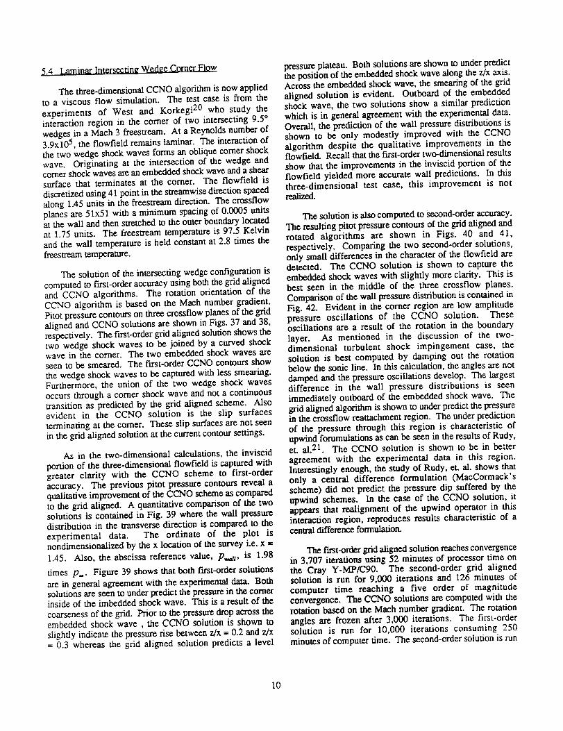
5,4 Laminar Intersecting Wedge Comer Flow

The three-dimensional CCNO algorithm is now appliedto a viscous flow simulation. The test case is from the

experiments of West and Korkegi 20 who study theinteraction region in the corner of two intersecting 9.5*wedges in a Math 3 freestream. At a Reynolds number of3.9x105, the flowfield remains laminar. The interaction of

the two wedge shock waves forms an oblique comer shockwave. Originating at the intersection of the wedge andcomer shock waves are an embedded shock wave and a shearsurface that terminates at the corner. The flowfield is

discretized using 41 point in the streamwise direction spacedalong 1.45 units in the freestream direction. The crossflowplanes are 51x51 with a minimum spacing of 0.0005 unitsat the wall and then stretched to the outer boundary locatedat 1.75 units. The freestream temperature is 97.5 Kelvinand the wall temperature is held constant at 2.8 times thefreestream temperature.

The solution of the intersecting wedge configuration iscomputed to first-order accuracy using both the grid alignedand CCNO algorithms. The rotation orientation of theCCNO algorithm is based on the Mach number gradient.Pitot pressure contours on three erossflow planes of the gridaligned and CCNO solutions are shown in Figs. 37 and 38,respectively. The In'st-order grid aligned solution shows thetwo wedge shock waves to be joined by a curved shockwave in the corner. The two embedded shock waves areseen to be smeared. The first-order CCNO contours show

the wedge shock waves to be captured with less smearing.Furthermore, the union of the two wedge shock wavesoccurs through a comer shock wave and not a continuoustransition as predicted by the grid aligned scheme. Alsoevident in the CCNO solution is the slip surfacesterminating at the corner. These slip surfaces are not seenin the grid aligned solution at the current contour settings.

As in the two-dimensional calculations, the inviscidportion of the three-dimensional flowfield is captured withgreater clarity with the CCNO scheme to first-orderaccuracy. The previous pitot pressure contours reveal aqualitative improvement of the CCNO scheme as comparedto the grid aligned. A quantitative comparison of the twosolutions is contained in Fig. 39 where the wall pressuredistribution in the transverse direction is compared to theexperimental data. The ordinate of the plot isnondimensionalized by the x location of the survey i.e. x =

1.45. Also, the abscissa reference value, p_,, is 1.98

times p.. Figure 39 shows that both first-order solutions

are in general agreement with the experimental data. Bothsolutions are seen to under predict the pressure in the cornerinside of the imbedded shock wave. This is a result of the

coarseness of the grid. Prior to the pressure drop across theembedded shock wave, the CCNO solution is shown toslightly indicate the pressure rise between z/x = 0.2 and z/x

= 0.3 whereas the grid aligned solution predicts a level

pressure plateau. Both solutions are shown to under predictthe position of the embedded shock wave along the z/x axis.Across the embedded shock wave, the smearing of the gridaligned solution is evident. Outboard of the embeddedshock wave, the two solutions show a similar predictionwhich is in general agreement with the experimental data.Overall, the prediction of the wall pressure distributions isshown to be only modestly improved with the CCNOalgorithm despite the qualitative improvements in theflowfield. Recall that the first-order two-dimensional results

show that the improvements in the inviscid portion of theflowfield yielded more accurate wall predictions. In thisthree-dimensional test case, this improvement is notrealized.

The solution is also computed to second-order accuracy.The resulting pitot pressure contours of the grid aligned androtated algorithms are shown in Figs. 40 and 41,respectively. Comparing the two second-order solutions,only small differences in the character of the flowfield aredetected. The CCNO solution is shown to capture theembedded shock waves with slightly more clarity. This is

best seen in the middle of the three crossflow planes.Comparison of the wall pressure distribution is contained inFig. 42. Evident in the comer region are low amplitudepressure oscillations of the CCNO solution. Theseoscillations are a result of the rotation in the boundarylayer. As mentioned in the discussion of the two-dimensional turbulent shock impingement case, thesolution is best computed by damping out the rotationbelow the sonic line. In this calculation, the angles are notdamped and the pressure oscillations develop. The largestdifference in the wall pressure distributions is seenimmediately outboard of the embedded shock wave. Thegrid aligned algorithm is shown to under predict the pressurein the crossflow reattachment region. The under prediction

of the pressure through this region is characteristic ofupwind forumulations as can be seen in the results of Rudy,et. al.21. The CCNO solution is shown to be in be:ter

agreement with the experimental data in this region.Interestingly enough, the study of Rudy, et. al. shows thatonly a central difference formulation (MacCormack'sscheme) did not predict the pressure dip suffered by theupwind schemes. In the case of the CCNO solution, itappears that realignment of the upwind operator in thisinteraction region, reproduces results characteristic of acentral difference formulation.

The fast-order grid aligned solution reaches convergencein 3,707 iterations using 52 minutes of processor time onthe Cray Y-MP/C90. The second-order grid alignedsolution is run for 9,000 iterations and 126 minutes ofcomputer time reaching a five order of magnitude

convergence. The CCNO solutions are computed with therotation _ on the Math number gradient. The rotationangles are frozen after 3,000 iterations. The first-ordersolution is run for 10,000 iterations consuming 250minutes of computer time. The second-order solution is run

10

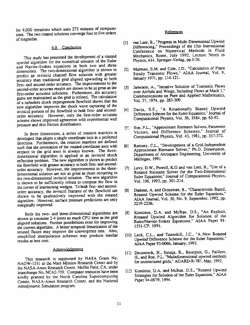
for 9,000iterationswhichuses273minutesof computertime.Thetworotatedsolutionsconvergefourtofiveordersofmagnidue.

[i]

This study has presented the development of a rotatedupwind algorithm for the numerical solution of the Eulerand Navier-Stokes equations in both two and threedimensions. The two-dimensional algorithm is shown to [2]

predict an inviscid channel flow solution with greateraccuracy than traditional grid aligned upwinding to bothfn'st- and second-order accuracy. The improvements to thesecond-order accurate results are shown to be as great as the [3]t%rst-order accurate solutions. Futhermore, the accuracygains are maintained as the grid is refined. The calculationof a turbulent shock impingement flowfield shows that thenew algorithm improves the shock wave capturing of theinviscid portion of the flowfield to both f'trst- and second- [4]order accuracy. However, only the fast-order accuratescheme shows improved agreement with experimental wallpressure and skin friction distributions.

[51In three dimensions, a series of rotation matrices is

developed that aligns a single coordinate axis in a preferreddirection. Furthermore, the rotation matrices are definedsuch that the orientation of the rotated coordinate axes with [6]respect to the grid axes is always known. The three-dimensional algorithm is applied to an inviscid shockreflection problem. The new algorithm is shown to predictthe flowfield with greater accuracy to both f'trst- and second-order accuracy. However, the improvements to the three- [7]dimensional solution are not as great as those occurring inthe two-dimensional inviscid solution. The new algorithmis shown to be sufficiently robust to compute the flow inthe corner of intersecting wedges. To both Fast- and second-order accuracy, the inviscid features of the flowfield are [8]shown to be qualitatively improved with the rotatedalgorithm. However, surface pressure predictions are onlymarginally improved.

Both the two- and three-dimensional algorithms are [9]shown to consume 2-4 times as much CPU time as the gridaligned solutions. Further possibilities exist for improvingthe current algorithm. A better temporal linearization of therotated fluxes may improve the convergence rate. Also,simplified interpolation schemes may produce similar [10]results at less cost.

This research is supported by NASA Grant No.NAGW-1331 to the Mars Mission Research Center and bythe NASA-Ames Research Center, Moffet Field, CA, underInterchange No. NCA2-719. Computer resources have been

kindly granted by the North Carolina SupercomputingCenter, NASA-Ames Research Center, and the National

Aerodynamic Simulation program.

[11]

[12]

References

van Leer, B., "Progress in Multi-Dimensional UpwindDifferencing," Proceedings of the 13th InternationalConference on Numerical Methods in Fluid

Mechanics, Rome, July 1992, Lecture Notes inPhysics, 414, Springer-Verlag, pp.l-26.

Murman, E.M. and Cole, J.D., "Calculation of Plane

Steady Transonic Flows," AIAA Journal, Vol. 9,January 1971, pp. 114-121.

Jameson, A., "Iterative Solution of Transonic Flows

over Airfoils and Wings, Including Flows at Mach 1,"Communications on Pure and Applied Mathematics,Vol. 27, 1974, pp. 283-309.

Davis, S.F., "A Rotationally Biased UpwindDifference Scheme for the Euler Equations," Journal ofComputational Physics, Vol. 56, 1984, pp. 65-92.

Roe, P.L., "Approximate Riemann Solvers, ParameterVectors, and Difference Schemes," Journal of

Computational Physics, Vol. 43, 1981, pp. 357-372.

Rumsey, C.L., "Development of a Grid-IndependentApproximate Riemann Solver," Ph.D. Dissertation,Department of Aerospace Engineering, University ofMichigan, 1991.

Levy, D.W., Powell, K.G and van Leer, B., "Use of aRotated Riemann Solver for the Two-Dimensional

Euler Equations," Journal of Computational Physics,Vol. 106, 1993, pp. 201-214.

Dadone, A. and Grossman, B., "Characteristic-Based,

Rotated Upwind Scheme for the Euler Equations,"AIAA Journal, Vol. 30, No. 9, September, 1992, pp.2219-2226.

Kontinos, D.A. and McRae, D.S., "An Explicit,Rotated Upwind Algorithm for Solution of theEuler/Navier-Stokes Equations," AIAA Paper 91-1531-CP, 1991.

Leek, C.L., and Tannehill, J.C., "A New Rotated

Upwind Difference Scheme for the Euler Equations,"A/AA Paper 93-0066, January, 1993.

Deconinck, H., Struijs, R., Bourgois, G., Paillere,H., and Roe, P.L. "Mulitdimensional upwind methodsfor unstructured grids," AGARD-R-787, May, 1992.

Kontinos, D.A. and McRae, D.S., "Rotated UpwindStrategies for Solution of the Euler Equations," AIAAPaper 94-0079, 1994.

11

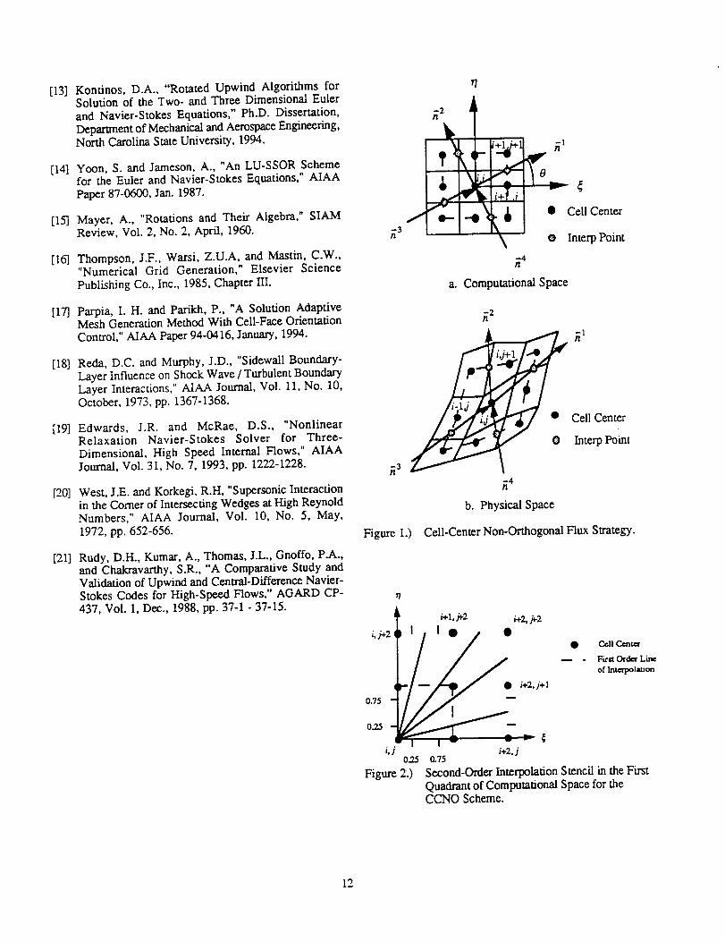
[13]

[14]

[15]

[16]

[17J

[18]

[19]

[20]

Kontinos, D.A., "Rotated Upwind Algorithms forSolution of the Two- and Three Dimensional Eulerand Navier-Stokes Equations," Ph.D. Dissertation,Department of Mechanical and Aerospace Engineering,North Carolina State University, 1994.

[21]

Yoon, S. and Jameson, A., "An LU-SSOR Schemefor the Euler and Navier-Stokes Equations," AIAAPaper 87-0600, Jan. 1987.

Mayer, A., "Rotations and Their Algebra," SIAMReview, Vol. 2, No. 2, April, 1960.

Thompson, J.F., Warsi, Z.U.A, and Mastin, C.W.,"Numerical Grid Generation," Elsevier SciencePublishing Co., Inc., 1985, Chapter III.

Parpia, I. H. and Parikh, P., "A Solution AdaptiveMesh Generation Method With Cell-Face OrientationControl," AIAA Paper 94-0416, January, 1994.

Reda, D.C. and Murphy, J.D., "Sidewall Boundary-Layer Influence on Shock Wave / Turbulent BoundaryLayer Interactions," AIAA Journal, Vol. 11, No. 10,October, 1973, pp. 1367-1368.

Edwards, J.R. and McRae, D.S., "NonlinearRelaxation Navier-Stokes Solver for Three-Dimensional, High Speed Internal Flows," AIAAJournal, Vol. 31, No. 7, 1993, pp. 1222-1228.

West, J.E. and Korkegi, R.H, "Supersonic Interactionin the Comer of Intersecting Wedges at High ReynoldNumbers," AIAA Journal, Vol. 10, No. 5, May,1972, pp. 652-656.

Rudy, D.H., Kumar, A., Thomas, J.L., Gnoffo, P.A.,and Chakravarthy, S.R., "A Comparative Study andValidation of Upwind and Central-Difference Navier-Stokes Codes for High-Speed Flows," AGARD CP-437, Vol. 1, Dec., 1988, pp. 37-1 - 37-15.

-3/1

J

-z An

¥ I

• Cell Centere-- I -O tl- II II

_ 0 Interp Point

-4/I

a. Computational Space

-2

_,/ Cell CenterInterp Point

_3-4/1

b. Physical Space

Figure I.) Cell-Center Non-Orthogonal Flux Strategy.

i+1,_-2 i+2, .h-2

°" i-t.z5__

i,j i+2, i0.25 0.75

Figure2.)

• Ce.II Camt_-

- Vtrg Order Line

of Intcrpolaticc

Second-Order Imcrpolation Stencil in the FirstQuadrant of Computational Space for theCCNO Scheme.

12

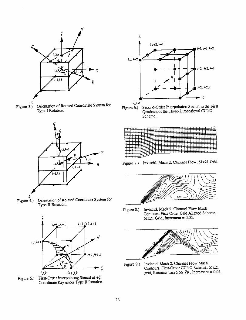
Figure 3.)

,

Orientation of Rotated Coordinate System for

Type I Rotation.

/Figure 4.) Orientation of Rotated Coordinate System for

Type Ii Rotation.

l i,/+l_+l i+1#1_+11

id,k i+I j,k

Figure 5.) First-Order Interpolating Stencil of+_'Coordinate Ray under Type II Rotation.

i,j,k

Figure 6.)

T i,j+2, k+2•/ -i,j,k+2 ,_'_/+2../+2. k+2

I I

I I)/

I .I I

7 ,,_ i+2, j+2,k

Second-Order Interpolation Stencil in the FirstQuadrant of the Three-Dimensional CCNOScheme.

Figure 7.)

Figure 8.) Inviscid, Mach 2, Channel Flow Mach

Contours, First-order Grid Aligned Scheme,61x21 Grid, Increment = 0.05.

Figure 9.) Inviscid, Mach 2, Channel Flow MachContours, First-Order CCNO Scheme, 61x21

grid, Rotation based on Vp, Increment = 0.05.

13

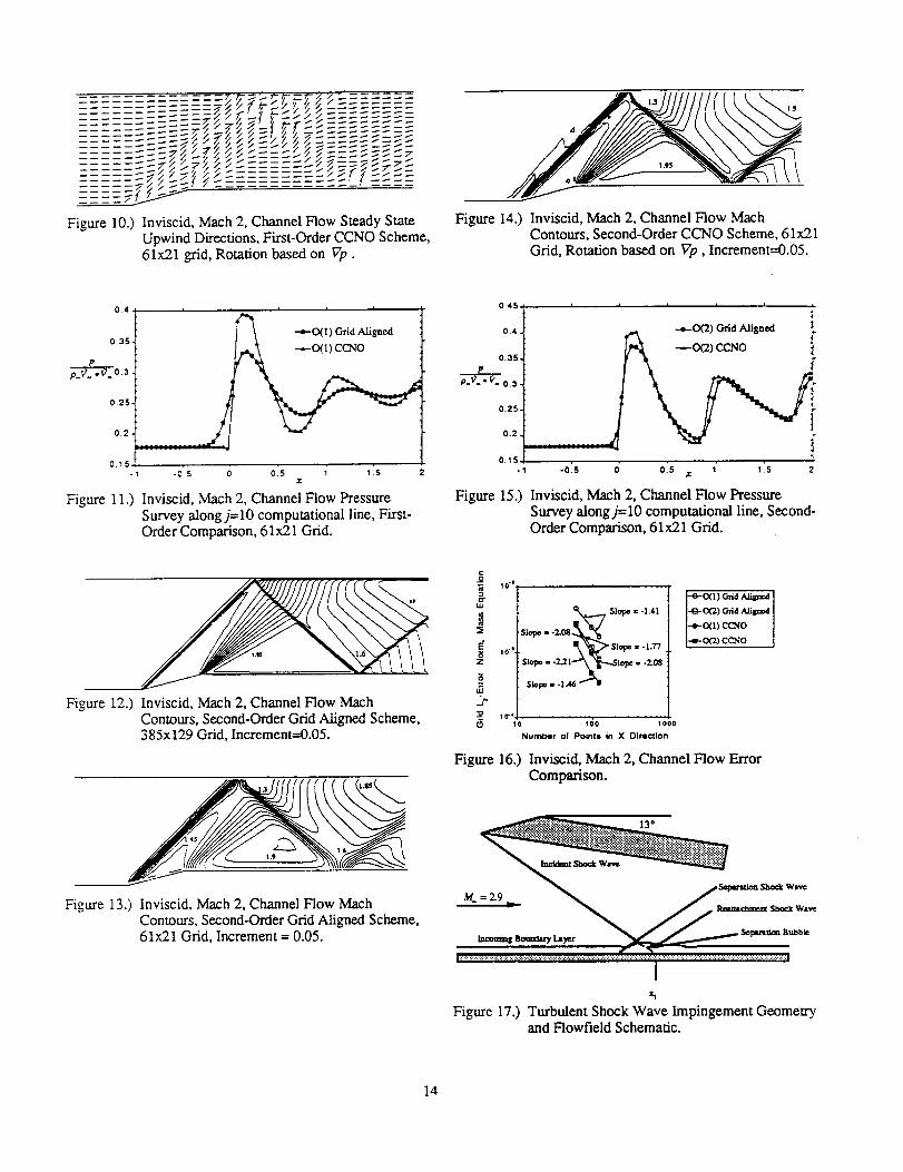
........ -- "<" " f T, _ _, r. /. ............ _X>" ,f--_ _-/// ....... --

7 _ ....

Figure 10.) Inviscid, Mach 2, Channel Flow Steady StateUpwind Directions, First-Order CCNO Scheme,61x21 grid, Rotation based on Vp.

Figure 14.) Inviscid, Mach 2, Channel Flow MachContours, Second-Order CCNO Scheme, 61x21Grid, Rotation based on Vp, Increment=0.05.

04

0.35

P

p_,,7 ._7. 0.3,

0.25-

02.

0.151

i i i i

_0(I) Grid Aligned

_r

Figure 11.) Inviscid, Mach 2, Channel Flow PressureSurvey alongj=10 computational line, First-Order Comparison, 61x21 Grid.

0.45 ,,. I I i i i

0.4. _ -4-0(2) Grid Aligned

0.35.

._...e__ep.V ._. o.a.

0,25-

0.2

0.15 .

-_ -o:s o' o:s _ ? _:s 2

Figure 15.) Inviscid, Math 2, Channel Flow PressureSurvey alongj=lO computational line, Second-Order Comparison, 61x21 Grid.

Figure 12.) Inviscid, Mach 2, Channel Flow Mach

Contours, Second-Order Grid Aligned Scheme,385x129 Grid, Increment---O.05.

Figure 13.) Inviscid, Mach 2, Channel Flow Mach

Contours, Second-Order Grid Aligned Scheme,61x21 Grid, Increment = 0.05.

10"'

g10".

Z

B

U,J

_2 tO''.

..7 S)ap¢ = -1.41

-e-off) C_d _ ]

-_-(X2) Gala Alilp_ I

-_-0(I) CC'qO I

-_- oa) cc_o j

(_ 10 100 1000

Number of Points in X Direction

Figure 16.) Inviscid, Math 2, Channel Flow ErrorComparison.

i_._.........................;...........................................,................. ¢7... _ -- I

Ixt

Figure 17.) Turbulent Shock Wave Impingement Geometryand Flowfield Schematic.

14

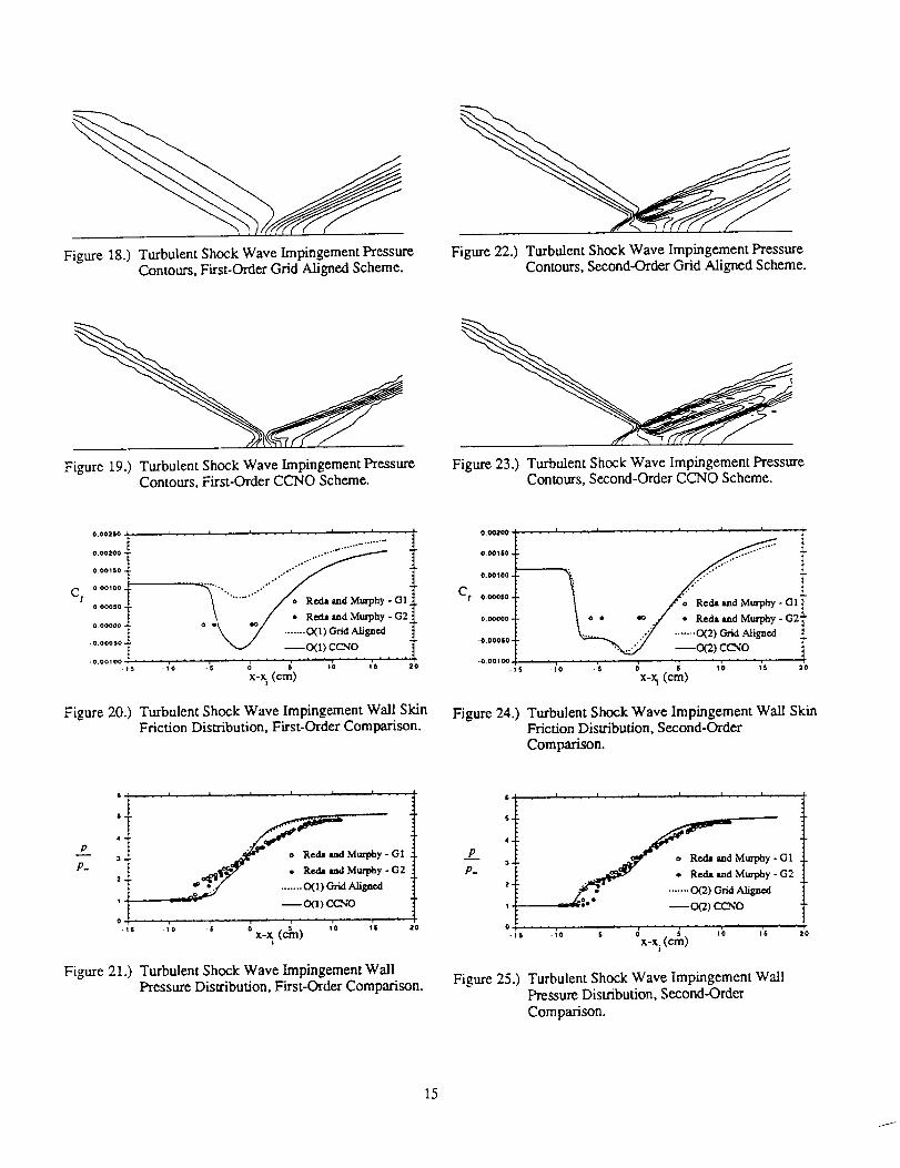
Figure18.)TurbulentShockWaveImpingementPressureContours,First-OrderGridAlignedScheme.

Figure22.)TurbulentShockWaveImpingementPressureContours,Second-OrderGridAlignedScheme.

Figure19.)TurbulentShockWaveImpingementPressureContours,First-OrderCCNOScheme.

Figure23.)TurbulentShockWaveImpingementPressureContours,Second-OrderCCNOScheme.

C t

0 [ O02SO i .... I [ . r I .... I _ 1 i . " r l . I . .

0.002000,001000.0..... ," t_"''"'" *'**'""" """'""'*'*"'"""*'"_"'**_" .......

o.oooso. - GI

02" ,o / *Red., and Murphy - G2

o.ooooo * _ ....... (9(1) (3_d A/i_l)c.d.O.O00SO-

_o(1) CCNO• O.O01QO ; ............. , , , , , , ...... ,

.,, .;o % x-x (era)

Figure 20.) Turbulent Shock Wave Impingement Wall SkinFriction Distribution, First-Order Comparison.

0.002_ . [ q _ .... I i . I . 1 t I .... I ....

0,001S0 , ...,"'"'"

C#. 0.0010@ • "_" _..'""O.O001_O • ""

oooooot o. "t •-o.oooso- k:_ ../ ...... 0(2) Grid Aligned

--cx2) cc,_o.0.00100 ........ _ - _ , - . . _ .... , .... , . .

-lS -1'0 .5 0 $ 10 IS ' ;

x-_ (cm)

Figure 24.) Turbulent Shock Wave Impingement Wall SkinFriction Distribution, Second-OrderComparison.

6 i . I I . I . . I .... i " I ....

P.3. Murphy - GI

,,¢jf"j • _,,,_ _,J M,_y - o2

1

: _ 0(1)C,CNO0 - - , ........... , .... . - , • , . .

" '° '_ _x-_ (elrl) '0 "20

Figure 21.) Turbulent Shock Wave Impingement Wall

Pressure Distribution, First-Order Comparison.

4,

p7. 3.

2-

.... I .... i I . . I I I .

1-

0

-1S .(0 /S

_z7.: ......0,:2)o.<,_,.__'* -- CK'/)CCNO

d 5 IO (& 20

X-Xi(era)

Figure 25.) Turbulent Shock Wave Impingement WallPressure Distribution, Second-Order

Comparison.

15

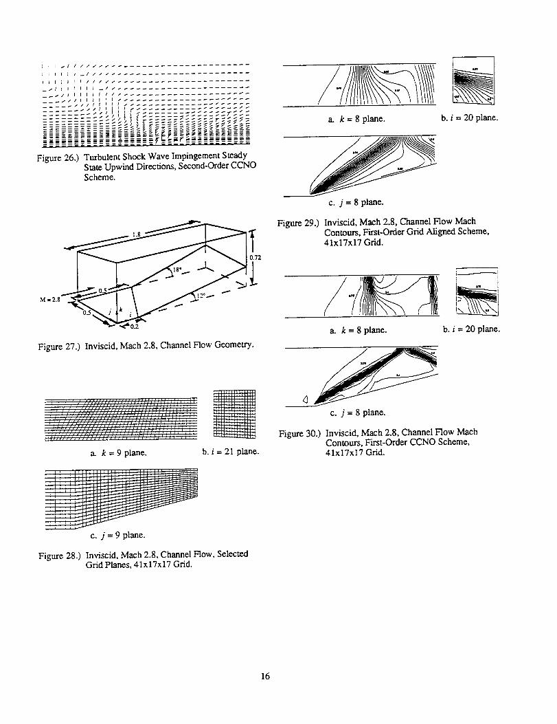
IIIJAPIII//I_ .....................

_xlIlldll_Ix1_ ...................

"¢_}I _z''c===zzz=:;;zc-:_;

NNNNNNNNNNNN_NNN_

Figure 26.) T_bulent Sh_k Wave Impingement S_adySm_ Upwind D_om, S_ond-Order CCNOScheme.

M_2.g_ _

0.2

Figure 27.) Inviscid, Mach 2.8, Channel Flow Geometry.

; _' i,','//,'///,',,...... II///I/_;" _._ _c l "''l'/ ;i

," " " L ....

a. k = 9 plane. b. i = 21 plane.

a. k = 8 plane. b. i = 20 plane.

c. j = 8 plane.

Figure 29.) Inviscid, Mach 2.8, Channel Flow MachContours, First-Order Grid Aligned Scheme,41x17x17 Grid.

a. k --8 plane. b. i = 20 plane.

c. j = 8 plane.

Figure 30.) Inviscid, Mach 2.8, Channel Flow MachContours, First-Order CCNO Scheme,41x17x17 Grid.

c. j = 9 plane.

Figure 28.) Inviscid, Mach 2.8, Channel Flow, SelectedGrid Planes, 41x17x17 Grid.

16

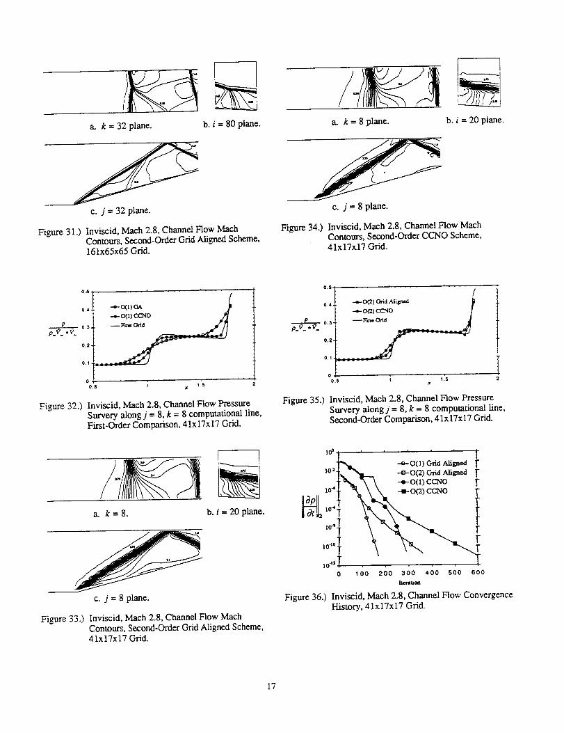
a. k = 32 plane.

c. j = 32 plane.

Figure 31.)

b. i = 80 plane.

Inviscid, Mach 2.8, Channel Flow Mach

Contours, Second-Order Grid Aligned Scheme,161x65x65 Grid.

a. k = 8 plane.

c. j = 8 plane.

Figure 34.) Inviscid, Mach 2.8, Channel Flow MachContours, Second-Order CCNO Scheme,41x17x17 Grid.

b. i = 20 plane.

p._.-_

0.5

0.4

0.3,

0.2.

0.1.

00.5

J _ _ . , . _ _

--_ o(1) c,A

1 .'5x

Figure 32.) Inviscid, Mach 2.8, Channel Flow PressureSurvery along j = 8, k = 8 computational line,First-Order Comparison, 41xlTx17 Grid.

O.S

0,4.

0.3-

p._. -_.

0.2-

0.1

0

0,5 1 1.5z

Figure 35.) Inviscid, Mach 2.8, Channel Flow PressureSurvery alongj = 8, k = 8 computational line,Second-Order Comparison, 41x17x17 Grid.

a. k=8. b. i = 20 plane.

c. j = 8 plane.

Figure 33.) Inviscid, Mach 2.8, Channel Flow Mach

Contours, Second-Order Grid Aligned Scheme,41x17x17 Grid.

lO ° , , i _ ,

" --Q-O(1) Grid AlignedZO=- --_-O(2) Grid Aligned

" .-e- 0(1) CCNO

10"4" _0

0 1 O0 200 300 400 500 600

|rcrtuon

Figure 36.) Inviscid, Mach 2.8, Channel Flow ConvergenceHistory, 41x17x17 Grid.

17

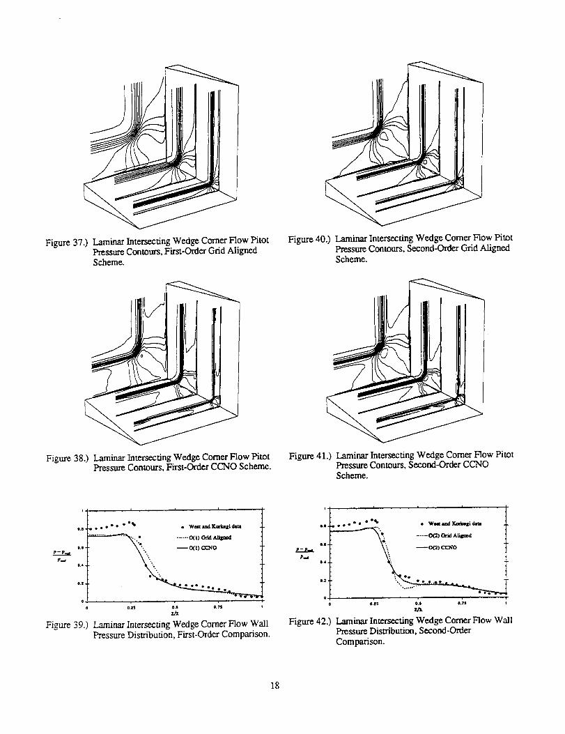
Figure 37.) Laminar Intersecting Wedge Comer Flow PitotPressure Contours, First-Order Grid AlignedScheme.

Figure 40.) Laminar Intersecting Wedge Comer Flow PitotPressure Contours, Second-Order Grid AlignedScheme.

Figure 38.) Laminar Intersecting Wedge Comer Flow PitotPressure Contours, First-Order CCNO Scheme.

Figure 41.) Laminar Intersecting Wedge Comer Flow PitotPressure Contours, Second-Order CCNOScheme.

i . . . i . i i

o.e • • • • • • eee • Wll_lml_lKtl'blle|d41141

_..'. ------_)_

P,..r o.4°'* _ _0(11 ¢1_O

O.2,

• • ee ee

o

0._ O.S O,?S

Figure 39.) Laminar Intersecting Wedge Comer Flow WallPressure Dis_ibution, First-Order Comparison.

) 1 _ m i . _

o.8. ,*_.. * Wotsnd Kmkali

...... (_.) _ia A_do.1_.

:. _o_) cc_oP,=d

e,2 - '.. eo

o

OmZ5 O.S 0.TS

z/x

Figure 42.) Laminar Intersecting Wedge Comer Flow WallPressure Distribution, Second-OrderComparison.

18

Technical Publications Resulting fromThis Cooperative Research

Kontinos, D. A. and McRae, D. S., "Rotated Upwind Strategies for Solution of the Euler

Equations", AIAA 94-0079, 32nd Aerospace Sciences Meeting, Reno, NV, January, 1994.

Kontinos, D. A. and McRae, D. S., "Rotated Upwind Algorithms for Solution of the Two-and Three-Dimensional Euler and Navier-Stokes Equations", AIAA 94-2291, 25th AIAA FluidDynamics Conference, Colorado Springs, CO, June 20-23, 1994.

Kontinos, D. A., "Rotated Upwind Algorithms for Solution of the Two-and Three-Dimensional Euler and Navier-Stokes Equations", Ph.D. Dissertation, N.C. State University,Spring, 1994.