University of Plymouth

PEARL https://pearl.plymouth.ac.uk

04 University of Plymouth Research Theses 01 Research Theses Main Collection

1985

THE DEVELOPMENT AND

ASSESSMENT OF AN ANALYTICAL

STRUCTURAL MAINTENANCE

DESIGN SYSTEM FOR ROADS

KUMAR, V. BALA

http://hdl.handle.net/10026.1/2804

University of Plymouth

All content in PEARL is protected by copyright law. Author manuscripts are made available in accordance with

publisher policies. Please cite only the published version using the details provided on the item record or

document. In the absence of an open licence (e.g. Creative Commons), permissions for further reuse of content

should be sought from the publisher or author.

THE DEVEI..DPMENT AND ASSESSMENT OF AN ANALYTICAL srRUCIURAL MAINTENANCE

DESIGN SYSTEM FOR IDADS.

by

V. BALA KUMAR, B.Sc .

This thesis is suhn.itted to the CoLIDcil for National Academic Awards in

partial fulfilment of the requirements for the Degree of Doctor of

Philosophy.

This work was LIDdertaken within the Department of Civil Engineering at

Plyrcouth Polytechnic, Plyrcouth, in collaroration with the Transport and

Road Research Laboratory (TRRL), U.K ••

September 1985

ABSTRACI'.

Previous work at Plynouth has shown the deflected shape as measu­

red by the Deflectograph can be used to estimate the thickness of surfa­

cing. This thesis extends the earlier work to develop relations between

deflected shape and the stiffness and thickness of pavement layers.

A literature study has been carried out to identify the factors

causing the deterioration of flexible pavements. The literature study

also assesses the various pavement evaluation equipnent that is available

and describes various methods of analysis and the interpretation of the

pavement surface deflection shape 1 that have been prop:>sed. The propert­

ies of the materials of the various layers of the flexible pavement have

been reviewed. Various structural rrodels of a pavement are considered and

the study indicates that the finite element method provides a most accur­

ate prediction of actual pavement response to a moving wheel load.

A 3D finite element rrodel of a flexible pavement has been prodoced

and partially validated with data obtained fran the TRRL. A Fortran Prog­

rame has been developed to convert absolute deflections predicted by the

3D rrodel into equivalent Deflectograph deflections. The rrodel has been

used to carry out parametric study to establish appropriate relationships

between the deflected shape and material properties of the pavement

layers. Relationships have been established to determine the thickness 1

nodular ratio and nodulus of the pavement layers and its supp:>rt subgrade

fran rreasurement of the deflected shape. An Analytical Pavement Evaluat­

ion and Design System has been set up based on the relationships. The

system has been validated by ccrnparing the material properties obtained

fran the laboratory testing with those predicted by the design rrodel

using the Deflectograph measurements obtained fran local roads with

measurerrent of layer thickness and subgrade strength measured in-si tu.

ABSTRACI'.

Previa.ts work at Plyrrouth has sh:Jwn the deflected shape as measu­

red by the Deflectograph can be used to estimate the thickness of surfa­

cing. This thesis extends the earlier work to develop relatioos between

deflected shape and the stiffness and thickness of pavenent layers.

A literature study has been carried out to identify the factors

causing the deterioration of flexible pavanents. The literature study

also assesses the various pavanent evaluation equi:pnent that is available

and describes various methods of analysis and the interpretation of the

pavement surface deflectioo shape 1 that have been prop:>sed. The propert­

ies of the materials of the various layers of the flexible pavement have

been reviewed. Various structural rrodels of a pavanent are considered and

the study indicates that the finite elanent method provides a rcost accur­

ate predictioo of actual pavement response to a rroving Wheel load.

A 3D finite element rrodel of a flexible pavement has been prcrlu:ed

and partially validated with data obtained fran the TRRL. A Fortran Prcxr

rame has been developed to convert absolute deflections predicted by the

3D rrodel into equivalent Deflectograph deflections. The rrodel has been

used to carry out parametric study to establish appropriate relationships

bet....een the deflected shape and material properties of the pavenent

layers. Relationships have been established to detennine the thickness 1

rrodular ratio and rrodulus of the pavement layers and its supp;::>rt subgrade

fran measurement of the deflected shape. An Analytical Pavement Evaluat­

ion and Design System has been set up based eo the relationships. The

system has been validated by canparing the material properties obtained

fran the laboratory testing with those predicted by the design rrodel

using the Deflectograph measurements obtained fran local roads with

measurement of layer thickness and subgrade strength measured in-si tu.

DECLARATION.

While registered as a candidate for the degree for which this

submission is made, the author has not been a registered candidate £or

another award of the C. N.A.A. or of a University during the research

prograrnne.

All -....K)rk described in this thesis is wholly original and was

carried out by the author except where specifically noted by reference.

Assistance received in the research -....K)rk and perparation of this thesis

is acknowledged.

Author: V. BAIA r<:uMAR •

........... ~!', ..... Supervisor: Pro£. C. K. KENNEDY.

ACKNOWLECGMENTS.

The author is indebted to the Science Engineering and Research

cowcil (SERC) for its financial supfX)rt. The author wishes to express

his graditude in particular to Pro£. C.K.Kennedy, Head of Department of

Civil Engineering, Plyrrouth Polytechnic, who supervised this thesis and

who gave generously of his time for discussion and supfX)rt.

Thanks are due to Dr. I. Butler, Mr. B. Undy and Mrs. P . Hop.vcod

for their help. Thanks are also due to Mr. D.Hicks and Mr. G.Bouch of

the Canp.1ter centre for their help.

SI'ATEMENT OF ADVANCED SIUDIES.

The author has, during his period of research, attended tYJI',)

residential courses: 'Symp:Jsiurn on Highway Maintenance and Data Colle­

ction', held at Nottingham University in July 1983, and 'Analytical

Design of Bi turninous Pavements' , held at Nottingham University in April

1984.

The author has written a paper to the International SymfOsium

on 'The Bearing Capacity of Roads and Airfields' to be held in Sept

1986 at Plymouth.

The author has attended the course entitled 'The Deflectograph

Use and Analysis of Results', organised by the Department of Civil

Engineering at Plyrrouth Polytechnic for practising enginners.

The author attended the 'European Flexible Pavement Study

Group Meeting' held at Plymouth Polytechnic in July 1983.

LIST OF FIGURES.

LIST OF TABLES.

LIST OF PlATES.

NOI'ATIONS.

TABLE OF <X>NTENTS.

Page

ix

xiv

XV

xvi

CBAPI'ER 1 • 0 INrroOOcriON.

1.1 General.

1

1

1. 2 Factors Influencing The Deterioration

of Road Pavements. 2

1 • 2 .1 Traffic Loading. 2

1. 2. 2 Enviromtental Effects. 5

1.2.2.1 Moisture Content and Water Table. 5

1.2.2.2 Temperature. 5

-1 • 2 • 3 Design and Construction. 7

1. 3 Maintenance • 8

1.4 Statement of Problem. 9

1.5 Research HypOthesis. 9

rnAPI'ER 2.0 PAVEMENT EVAilJATION EQUIPMENT AND INI'ERPRETATION. 11

2.1 Introduction. 11

2. 2 Characterization of Measuring Device. 12

2.3 Rolling Wheel Techniques. 13

2.3.1 Deflection or Benkelman Beam. 14

2.3.1.1 Pavement Evaluation. 15

2 • 3. 2 Deflectograph. 18

2.3.2.1 Pavement Evaluation. 21

2.3.3 Travelling Deflectometer. 26

i

2.3.3.1 Pavement Evaluation.

2.3.4 CUrvature Meter.

2.3.4.1 Pavement Evaluation.

2 .4 Stationary Loading Techniques.

2.4.1 Plate Bearing Test.

2.4.1.1 Pavement Evaluation.

2.4.2 The Falling Weight Deflectameter.

2.4.2.1 Pavement Evaluation.

2.4.3 Dynaflect.

2.4.3.1 Pavement Evaluation.

2.4.4 Road Rater.

2.4.4.1 Pavement Evaluation.

2. 5 wave Propagation Technique.

2.5.1 Pavement Evaluation.

2.6 Factors Affecting The Selection of

Page

26

27

29

29

30

30

31

32

33

35

38

38

41

41

Pavement Evaluation Equipnent. 41

2. 7 Justification for the Selection of Deflectograph. 42

rnAPI'ER 3.0 MATERIAL OfARACI'ERIZATION FOR FLEXIBLE PAVEMENT DESIGN. 44

3 .1 Intoduction. 44

3.2 Bituminous Materials. 44

3. 2 • 1 Hot Rolled Asphalt ( HRA) • 45

3.2.2 Dense Bitt.nnen Macadam (DBM). 45

3. 2. 3 Open Textured Macadam. 46

3.3 Stiffness Characteristics. 46

3.3.1 Estimation of Bitt.nnen and Mix Stiffness. 47

3. 3 .1.1 Bi tt.nnen Stiffness. 4 7

3.3.1.2 Mix Stiffness. 50

ii

Page

3. 3. 2 Measured Stiffness. 53

3.3.2.1 Dynamic Test or Repeated

LOad TriaJCial Test. 54

3. 3 • 3 Pennanent Deformation . 60

3.3.3.1 Introduction. 60

3.3.3.2 Creep Testing. 60

3. 3. 3. 3 Repeated Load Testing. 63

3. 3. 4 Fatigue Cracking. 67

· 3.3.4.1 Introduction. 67

3.3.4.2 Effect of Stiffness and

Criterion of Failure. 67

3.3.4.3 Effect of Mix Variables. 69

3 • 3. 4. 4 Prediction of Fatigue Performance • 70

3.4 Cement Bound Materials. 72

3.5 COhesive Soil. 73

3.5.1 Resilient Behaviour. 74

3.5.2 Permanent Strain. 76

3.6 Granular Materials. 77

3. 6 .1 Resilient Behaviour. 78

3. 6. 2 Permanent Strain. 80

3. 7 Summary of Procedures to Detennine Material

Properties for Pavement Design.

3.7.1 Bituminous Material.

3.7.2 Cement Bound Materials.

3.7.3 COhesive Soil.

3.7.4 Granular Soil.

iii

80

81

82

82

83

Page

rnAPl'ER 4. 0 SELECI'ION OF STRUCIURAL MJDEL. 84

4 .1 Introduction • 84 .

4. 2 Linear Elastic Half-Space Theory. 84

4.2.1 EqUivalent Thickness Theory. 85

4. 3 Elastic Theory. 86

4.3.1 Layered Elastic Theory. 86

4. 3 .1.1 Elastic Theory Approach •. 89

4.3.2 Finite Element Method. 91

4.3.2.1 Finite Element Approach. 92

4.4 Visooelastic Layered System. 94

4.4.1 Visooelastic Approach. 95

4. 5 Theory Selection. 96

· rnAPl'ER 5.0 FINITE ELEMENT' ANALYSIS Of FLEXIBLE PAVEMENT. 99

5.1 Introduction. 99

5 • 2 The Finite Element Method • 99

5.2.1 Basic Structural Analysis. 100

5.2.2 Subdivision of Structure. 101

5.3 Finite Element Program (PAFEC). 102

5.3.1 Method of Analysis. 103

5.3.2 Basic Element Shapes. 104

5. 3. 3 'I\oio and Three Dimensional

Isoparametric Element. 106

5.3.4 Geometric Aspect Ratios of the Elements. 106

5. 3. 5 Autanatic Subcl i vision of Structure. 107

5.3.6 Material Properties. 108

5. 3.6.1 Incremental Procedure. 109

5.3.6.2 Iterative Procedure. 109

iv

5. 3 • 6 • 3 Mixed Procedure •

5.3.6.4 Oomparison of Basic Procedure.

5.3.6.5 Non-Linear Analysis -PAFEC.

5.3.7 Loadings.

5 • 4 Three Dimensional Pavanent.

5.4.1 M::ldel A.

5.4.2 M::ldel B.

5 • 4. 3 Conclusions to be Drawn fran 'I'he Initial

M::ldel A-B.

5.4.4 M::ldel c.

5.4.5 Model D.

5.4.6 Model E.

5.4.7 Model F.

5.5 Validation of the Final Model (M::ldel F).

5.5.1 Granular Road Base Pavanent.

5.5.1.1 Subgrade Layer.

5.5.1.2 Intermediate Granular Layer.

5.5.1.3 The Asphalt Bound Layer.

5.5.2 Matching the Response of the 3D Model

Page

110

110

111

111

112

115

117

122

123

124

126

133

138

138

139

140

140

And Actual Pavanent Structure. 143

5.5.3 Oomparison of Asphalt Tensile Stresses. 144

5. 6 FORI'RAN Program to Change the Absolute Deflection

to Deflectograph Deflection.

5.7 Stmnary.

V

151

152

OfAPI'ER 6.0 RELATIONSHIPS BE'IWEEN OJRVA'IURE AND/OR DEFLEcriON

AND THICKNESS AND ELASI'IC MJDUUJS OF THE VARIOUS

lAYERS OF THE PAVEMENT.

6.1 Introduction.

6.2 Parametric Study.

6.3 Selecting the Position of a Suitable Ordinate

Page

155

155

156

Differential Deflection. 158

6.4 Method of Statistical Analysis. 159

6.4.1 Regression and Fitting of Camon Slope. 160

6.4.2 Confidence Limit. 163

6. 5 Relationships Between Deflected Shape and

Pavement Condition.

6.5.1 Relationship Between o8 and CBR of

Subgrade.

6.5.2 Relationships Between Maximum Deflection,

o0 , and Equivalent Thickness, He.

6.5.3 Relationships Between o0-o8 and He

fiJr a Given Thickness of Granular Material,

fie (H2ffi3) •

6.5.4 Relationships Between o0-o8 and He

fiJr a Given Pavement Thickness,

Hp (HlffiG).

6.5.5 Relationships Between o0-o8 and He

for a Given Value E1/E2 Ratio.

6.5.6 Relationships Between o0-o2 and H1

for a Given Ratio E1/E2.

vi

163

163

166

170

171

174

175

6.5.7 Relationships Between o0-o2 and E1

for a Given Value of E2 and H1 •

Page

6.6 Analytical Pavanent Evaluation and Design System. 185

6.7 Limiting Factors. 185

6. 7.1 Insignificant Relationships. 186

6.8 Summary. 190

rnAPI'ER 7. 0 VALIDATION OF 'IHE ANALYTICAL PAVEMENT EVAilJATION

AND DESIGN SYSTEM.

7 .1 Introduction.

7. 2 Thickness and Modulus of Pavanent Layers.

7.2.1 Bituminous Material.

7 • 2. 2 Road Base Thickness and Subgrade strength.

7.3 Deflectograph Deflection (Input Values).

7.4 Limitation of Validation.

7. 5 Estimation of Thickness and Modulus

193

193

194

194

195

195

196

of Pavanent Layer. 196

7 • 5 .1 Estimation of Subgrade Strength, CBR. 196

7.5.2 Estimation of Equivalent Thickness, He· 197

7 • 5. 3 Estimation of Total Pavement Thickness,

Hp, and !bad Base Thickness, It. 197

7. 5. 4 Estimation of Modular Ratio E/E2 and

M::ldulus Values of E1 and E2 .

7.6 Canparison of Deflected Shape.

7.7 Conclusion.

vii

198

200

200

rnAPI'ER 8.0 SUMMARY, OONCI.lJSIONS AND REOJMMENDATIONS.

8 .1 Summary.

8.2 Conclusions.

8. 3 Recanmendations.

REFERENCFS.

APPENDIX I. EXXJIVALENT NODAL FORCES.

APPENDIX II • CONTACT' ARFA AND PRESSURE BmwEEN THE TYRE

AND THE OOAD.

APPENDIX Ill. PAFEC PRCX;RAM OF THE 3D l'ODEL.

APPENDIX IV. TRANS. F77 •

APPENDIX V. PLOT.F77.

APPENDIX VI • TABLES OF STATISTICAL ANALYSIS DErAilS.

APPENDIX VII. TRIAXIAL TESTING.

viii

Page

203

203

204

205

206

224

227

229

240

243

249

254

Lisr OF FIGURES.

Figure Page

1 .1 Developnent of Deformation in a Rolled Asphalt

Pavement and its Subgrade Related to Monthly

Temperature Durations within the Pavement. 6

1.2 Serviceability History. 9

1. 3 Effect of Maintenance. 9

2.1 Different Deflection Bowl fOr Same maximum Deflection. 12

2.2 Defining the 'Slope of Deflection'. 16

2.3 Cycle of Operation: Diagrarrmatic. 22

2.4 Diagrarrmatic Representation of Deflectograph. 23

2. 5 Essentail Chassis Details for Deflectograph Vehicles. 24

2.6 Recording the Deflected Shape as a Maximum Deflection

and Ten Ordinate Deflection. 25

2. 7 The Relationship Between the Maximum, Ordinate and

Differential Deflections. 25

2. 8 The curvarure Meter • 27

2.9 Recording Curvature with a Curvature Meter. 28

2.10 Deflection Interpretation Chart. 33

2.11 Dynaflect Deflection Basin Parameters. 35

3.1 Variation of Bitumen Stiffness with Time and Temperature. 47

3. 2 Narograph for Detennining the Stiffness of Bi tumens. 49

3.3 Loading Time as a Function of Vehicle Speed and Layer

Thickness. 50

3.4 Relationship Between Mix Stiffness and Binder Stiffness. 51

3. 5 Narograph fOr Mix Stiffness. 52

3.6 Stresses on a Soil Element due to a Passing Wheel Load. 55

3.7 Stress System in the Triaxial Test. 56

ix

Figure Page

3.8 Measurements in Repeated Load Triaxial Test with Constant

Cell Pressure.

3.9 Variation of Equivalent Vertical Stress Pulse Time with

Vehicle Velcx:i ty and Depth.

3.10 Creep Results.

3.11 COmparison of Results from Dynamic Tests aand Creep

0 Tests at 20 c.

3.12 Creep Tests-Effect of Stress Level.

3.13 Creep Tests-Effect of Temperature.

3.14 Influence of the Magnitude of the Vertical Stress Pulse

on Vertical Strain.

3 .15 Influence of Confining Stress on Vertical Strain.

3.16 Influence of Temperature on Vertical Strain.

3.17 Effect of Stiffness on Fatigue Life Using Different Modes

of Loading.

3 .18 Variation of Induced Stresses and Flexural Strength with

Elastic Modulus for Various Lean Concrete Bases.

3.19 The Effect of Stress Condition on the Resilient Modulus

of Cohesive Soil.

3.20 Resilient Modulus of a Saturated Silty Clay as a Function

of Deviator Stress.

3.21 Relationship Between Relative Compaction, Relative Moisture

Content and Resilient Modulus.

3.22 Relationship Between Permanent Strain and Number of

Stress Application for a Normally Consolidated Saturated

Silty Clay.

3.23 The Effect of Stress Condition on the Resilient Modulus

of Granular Soil •

X

57

58

61

62

63

63

65

66

66

71

73

73

74

76

77

79

Figure

3.24 Permanent Strain in a Granular Material as a Function

of Applied Stresses.

4.1 Diagramrntic Representation of the Equivalent Thickness

Theory.

Page

81

85

5.1 TWO Dimensional (2D) Elements. 105

5.2 Three Dimensional (3D) Elements. 105

5.3 Equivalent Nodal Loads due to Constant Pressures on

Element Surface. 112

5.4 Diagrammatic Representation of Deflectograph. 113

5.5 Absolute Deflection Profiles Along The Road. 114

5.6 Deflection Profiles Across The Road. 115

5.7 Deflectograph Tyre Print. 118

5.8 Triangles with: (a) curve Sides, and (b) Straight Sides. 118

5.9 Model Bl - B2. 119

5.10 Model B3 - 84.

5.11 Model c.

5.12 Model D.

121

127

128

5.13 Absolute Deflection of the Granular Roadbase Pavement. 129

5.14 Absolute Deflection of the Bitt.nninous Roadbase Pavement. 130

5.15 3D View of Model E.

5.16 Plan of Model E.

5.17 Finite Representation of Infinite Bodies.

5.18 Plan of Model F.

5.19 Various Layers of Model F.

5.20 Granular Road Base Pavement.

5.21 The Relationship Between Mix Stiffness, Binder Stiffness

and VMA.

xi

131

132

133

136

137

139

142

Figure Page

5.22 Elastic Modulus, Poisson' s Ratio and the Thickness of the

Initial Model. 143

5. 23 Elastic Modulus, Poisson' s Ratio and the Thickness of the

Final Model. 145

5. 24 Variation of the Subgrade Strength with Depth. 147

5.25 Comparison of Absolute Deflection Along the Line Through

the Centre of . the Twin Rear Wheels. 148

5.26 Comparison of Absolute Deflection Along the Line Through

the Centre of the Vehicle. 149

5. 27 Comparison of Deflectograph Deflection. 150

5.2B Simplified Diagrarnnatic Representation of Deflectograph. 152

6.1 Range of Layer Thickness and Elastic Modulus of Each Layer

of The Pavement. 15B

6.2 Nomenclature to Represent the Deflection Ordinates at

Various Distance away from the Point of Maximum Deflection 161

6. 3 Diagrarrmnatic Representation of the Methoo to Obtain the

Position and Distance of the Differential Deflection. 162

.6.4 Power Law Relationship Between DB and CBR.

6.5 scatter of Data: r..og10 (D0 ) Vs r..og10 (He) for CBR 2.

6.6 Relationships Between Do and He·

6.7 Relationships Between Do-DB and He for a Given HG· 6.B Relationships Between Do-DB and He for a Given ~·

6.9 Relationships Between Do-DB and He for CBR 2 for

Given E/E2 Ratio and E2

= 2 x lOB N/m2 •

6.10 Relationships Between D0-DB and He for CBR 2 for

Given E/E2 Ratio and E2 = 9 x lOB N/m2 •

6.11 Relationships Between D0-D8 and He for CBR 10 for

Given E/E2 Ratio and E2 = 2 x 108 N/m2 •

xii

165

16B

169

172

173

176

177

178

Figure

6.12 Relationships Between D0-D8 and He for CBR 10 for

Given E1/E

2 Ratio and E2 = 9 x 108 N/m2

•

6.13 Relationships Bet.v.een D0-D2 and H1 for Given Ratio

8 2 of E1/E2 and E2 = 2 x 10 N/m •

6.14 Relationships Between D0-D2 and H1 for Given &ltio

of E1/E2 and E2 = 9 x lOB N/rnF.

6.15 Relationships Bet.v.een D0-D2 and E1 for Given E2

and H1 = 100 mn.

6.16 Relationships Between D0-D2 and E1 for Given E2

and H1 = 150 mn.

6.17 Flow Chart: Analytical Pavement EValuation and Design

System.

6.17 Flow Chart: Analytical Pavement EValuation and Design

System ( a:mtinued) •

6.18 Relationships Bet.v.een D0-D3 and He for CBR 2 for

Given H1 •

Page

179

180

181

183

184

187

188

189

7 .1 Canparison of Deflectograph Deflection Profile: CBR 8. 201

7. 2 Canparison of Deflectograph Deflection Profile: CBR 11 • 202

A.l Change of Lateral PrOfile of Contact Pressure with

Inflation Pressure. 228

xiii

Lisr OF TABLES.

Table Page

1 .1 Reccmnended Standard AJcle Factor for Use in S .Africa. 4

2.1 Structural Diagnosis Chart Based on Dynaflect Deflections. 37

4 .1 Elastic Theories of 'I'wo Layered System. 88

4.2 Elastic Theories of Three Layered System. 88

5.1 Brief Description of Ten Phases of PAFEC 75. 103

5. 2 Warning, Error and Element Shape for 2D and 3D Elements. 122

5.3 Boundary Conditions of Model B. 125

5.4 Boundary Conditions of Model Cl - C2. 135

5. 5 Boundary Conditions of Model F. 135

5.6 General Infonnation about Model F. 146

5.7 Proportionality F,actor, Z, Derived fran The Shell Manual. 146

6.1 Different Combinations of the Thickness and Elastic Modulus

Modulus of the Different Layers of the Pavement. 157

6.2 Equations to Describe the Relationship Between Dg

and CBR. 164

6.3 Equations for the Relationships Between Do and He. 167

7.1 canparison of Thicknesses and Moduli of Pavement Layers. 199

A.l Statistical Analysis: Fitting of COTII'l'On Slope and

Confidence limit.

A. 2 Statistical Details of the PoY.er Law Relationship Between

D0-D8 and He for Given Thickness of Granular

Material, He;·

A.3 Equations to Describe the Relationships Between D0-D8

and He for a Given Value of Granular Material

Thickness, He; .

xiv

250

251

252

Table Page

A.4 Equations to Describe the Relationships Between D0

-D8

and He for a Given Pavement Thickness, ~.

A.5 Equations to Describe the Relationships Between D0-D8

and He for a Given Value of E/E2 ratio.

A.6 Equations to Describe the Relationships Between D0-D2

and H1 for a Given Value of E/E2 ratio.

A.7 Equations to Describe the Relationships Between D0

-D2

and E1 for a Given Value of E2 and H1 •

Lisr OF PLATES.

Plate

2.1 Deflectograph-Beam Assembly.

2.2 Deflectograph-Recording Head.

A.l Triaxial Testing System.

A.2 Vertical Displacement Transducer.

A.3 Lateral Displacement Collar and Transducer.

A.4 Deformation Measuring System.

XV

252

252

253

253

Page

20

23

25~

260

260

261

F

L

R

a

d

E

H. 1 ••• n

E. 1 ••• n

Jli. • .n

wl or dl

w2 or d2

w3 or d3

w4 or d4

ws or ds

D110

SCI

OCI

NJTATIONS.

= AXle Load Factor.

=AXle Load.

= Standard AXle Load.

= Radius of CurVature.

= Radius of Circular Loaded Area.

= Deflection.

= Deflection at Distance 0 m or Deflection at Centre of

Loaded Area.

= Poisson's Ratio.

= Elastic Modulus.

= Differential Deflection.

= Deflection at . Distance ' r' fran the Load.

= Ratio of the Deflection, dr, at a Distance 'r' fran

the Load to the Deflection Under the Centre of the

Load, d0

•

= Layer Thickness Layers i = 1 to n.

= Elastic Modulus of Layers i = 1 to n.

= Poisson's Ratio of Layers i = 1 ton.

= Deflection at Sensor No 1 .

= Deflection at Sensor No 2.

= Deflection at Sensor No 3.

= Deflection at sensor No 4.

= Deflection at Sensor No 5.

= Dynaflect Maximum Deflection (w1

).

= Surface curvature Index (1-41

- \-J2

) ·

= Bas2 Curvature Index (w4

- w5

) ·

xvi

SP%

HRA

D~

f

SP(or SP ) r

PI(or PI ) r

T

p

V

VMA

Evr

Err

Ep

M or E r r

/E/ *

acp

Ecp

= spreadibility [lOO(w1 + w2 + w3 + w4 + w5 )J

sw1

= Hot Rolled Asphalt.

= Dense Bitumen ~-1acadarn.

= Bitumen Stiffness.

= Mix Stiffness.

= Loading Time, sec.

= Frequency, Hz.

= Softening Point( or Recovered Softening Point), 0c.

= Penetration Index (or Recovered Penetration Index) ,

oc.

= Temperature, 0c.

= Penetration at 25 °c

= Vehicle Speed in Km/hr.

= Volume Concentration of the Aggregate.

= Volume of Voids.

= Voids in the Mixed Aggregate.

= Major Principal Stress.

= Minor Principal Stress = Cell Pressure = Applied

confining Pressure.

= AXial Strain.

= Radial Strain.

Permanent Strain.

= Resilient Modulus (Stiffness).

=Complex Modulus (Stiffness).

= Amplitude of the Sinusoidal Vertical Stress.

Amplitude of Resultant Sinusoidal Steady State Vertical

Strain.

xvii

a; a3

u

s

Ip

CBR

p

Esub:Jrade

q

qr

f)

X

y

z

Line XX

Line yy

= Phase Lag, oc.

= Time Lag Between a Cycle of Sinusoidal Stress and the

Resultant Cycle of Sinusoidal Strain, sec.

= Time for a Cycle of Sinusoidal Stress, sec.

= Service Life.

= Initial Strain Corresponding to a Given Number of

Cycle to Failure.

= Maximum Value of Applied Tensile Strain.

= Number of Cycles of Strain Applied.

= Number of Cycles to Produce Failure Under Constant

Strain Amplitude.

= Initial Effective Confining Stress.

= Applied Confining Stress.

= Initial Pore Pressure.

= Soil Suction •

= Plasticity Index, %.

= california Bearing Ratio.

= Mean Normal Stress.

= Elastic Modulus of Subgrade.

= Deviator Stress.

= Cyclic Deviator Stress.

= Sum of Principle Stress = Oj_ + 2 a2 = q + 3 a3

= 1 X1 Direction.

= 1 Y1 Direction.

= 1 z 1 Direction •

= Line Through the Centre of the Twin Rear Wheels

Near the Kerb.

= Line Through the Centre of the Vehicle.

xviii

Line zz

NS

os

2D

3D

D - D X y

= Line Through the Centre of the Twin Rear Wheels

Away fran the Kerb.

= Near Side Twin Rear Wheels of the Vehicle.

= Off Side Twin Rear Wheels of the Vehicle.

=Tyre Inflation Pressure.

= Actual Tyre Contact Area.

= Canp..1ted 'J:Yre Area •

= Static Wheel LOad.

= Two Dimensional.

= Three Dimensional.

= Equivalent Thickness;

Differential Deflection; Difference in Magnitude of

Deflection at Distances x and y away from the Point of

MaxUnum Deflection.

= Deflection at Distance x away fran the Point of

MaxUnum Deflection.

= Deflection at 0 rrm away from the Point of Maximum

Deflection.

= Deflection at 100 rrm away fran the Point of Maximum

Deflection.

= Deflection at 200 rrm away from the Point of MaxUnum

Deflection .

= Deflection at 300 rrm away from the Point of Maximum

Deflection.

= Deflection at 400 rrm away fran the Point of Maximum

Deflection.

xix

Ds = Deflection at 500 mn away fran the Point of Maximum

Deflection •

D6 = Deflection at 600 mn away fran the Point of Maximum

Deflection.

07 = Deflection at 700 mn away fran the Point of Maximum

Deflection.

Ds = Deflection at 800 mn away fran the Point of Naximum

Deflection •

HG = Thickness of the Granular Material.

11> = Thickness of the Pavement.

XX

rnAPTER 1 • 0 INI'OOOOcriON.

1 .1 General.

Structural deterioration under traffic takes place to same

extent in all road pavements although in well designed ones its

developnent is a very slow and seasonal process. An increasing propor­

tion of the network of major roads built in the last two decades will

require strengthening in the years ahead; this is o?.dditional to the

periodic strengthening required to improve the older and largely

undesigned road network, to maintain it at structural standards appro­

priate. to today's heavier traffic. It is therefore important that the

considerable expenditure~'on strengthening of roads should be made as

effective as possible by the use of a suitable method for designing

strengthening measures.

A system for the design of strengthening measures should be

capable of two functions:

(a) predicting the remaining life of a pavement under traffic so that

strengthening by overlaying can be tirred to coincide with the

onset of critical conditions;

(b) designing the thickness of overlay required to extend the life

of a road to carry any given traffic and to indicate length of

roads which have deteriorated sufficiently to require partial or

total reconstruction.

Essential to a design method is sane fonn of measurement of

the structural condition of the road. '!'he procedure must be sufficie­

ntly rapid and convenient to enable closely spaced measurements to be

made over long lengths of road in a realistic period of time.

1

The measurement of the surface deflection basin provides

valuable infonnation for the structural evaluation of flexible pave­

ments. The surface deflection of a pavement system and its curvature

under a load are influenced by the stiffness of its a:::mp:Jnent layers,

thickness, load intensity and its overall structural integrity. A

mechanistic rrethod of pavement design generally starts with a a:::mp:Jn­

ent analysis of the different materials (laboratory testing of mater­

ial specimens). The different a:::mp:Jnents are then incorp:>rated into a

system ( layered lllJdel) , and the behaviour of the whole system under

lead is analysed (stresses, strains, deflections). In a mechanistic

pavement evaluation rrethod, the system response is measured (surface

deflections) , the response is analysed with the use of a layered

lllJdel, and the material properties are back calculated.

1.2 Factors Influencing the Deterioration of Road Pavements.

1.2.1 Traffic Loading.

Both the magnitudes and the numbers of oammercial traffic

loads contribute to the damage of flexible pavements. For pavement

design purroses, it is usual to consider vehicle loadings in terms of

axle loads. Tyre pressure and wheel or axle configuration also influ­

ence the pavement performance. Defects caused by traffic include

fatigue cracking, defonnation, wear by loss or p:Jlishing of aggregate

and excessive embedment of chippings. ·

Tyre pressure primarily affects the wearing course and has

little influence on the loading of the lower layers. Wheel and axle

configurations influence mainly the upper layers of the pavement. The

AASHO (American Association of State Highway Officials) Road Test (l)

has shown that an 80 KN single axle load has the same structural

2

damaging effect as a 142 l<N tandem axle load, i.e. equivalent pavement

perfonnance achieved on similar pavement structure. A canplete system

of classifying cammercial traffic in tenns of vehicle types and axle

configurations is given in Ref (2).

Traffic on a road is mixed in ccrnrosition and therefore it is

very important for design purroses to express cumulative traffic in

tenns of an equivalent number of standard axles. Investigations were

carried out at the AASHO Road Test (1) to detennine the relative

damaging effects of loads of different sizes and the following relat-

ionship was developed:

F = (~ L

s

a (1.1)

The concept of equivalent load means that one application of

a load, L, is equivalent in tenns of pavement damage to, F, applicat-

ionsof a standard load, L , is generally taken as equal to 80 KN. s

The value of 'a' I£S found to be dependant uron the thickness of the

pavement and the strength of the subgrade but the average value from

the AASHO Road Test (1) I£S fotmd to be approximately 4.0. The relat-

ionship sh01r..n in Eqn 1.1 is also known as the Fourth Pov.er Law. Recent

work carried out in S.Africa (3) with a heavy vehicle simulator has

shOir.Kl that the value of 'a' can vary depending uron the pavement type

and the criterion of distress. The approximate equivalences obtained

for different pavement types is given in Table 1.1. A value of 4.2 was

recammended for use in S.Africa if an average value for all pavement

types was required •

The average equivalence factor suitable for use for flexible

pavements in the U.K. is given in Road Note 29 (4). If the ccrnrosition

of traffic is expressed in tenns of the number of axle loads in each

3

of a range of categories, the damaging pov.er of the traffic flow may

be assessed. The prornrtion of pavement damage caused by each load

category is obtained by multiplying the number of axle loads in that_

category by the appropriate equivalence factor. The equivalence factor

is used in. conjuction with measured load spectr<J. obtained fran weigh­

bridges installed in roads to assess the damaging power of tr<J.ffk of

<Hfferent oanrnsitions (5). The damaging effect of small axle loads is

insignificant despite their large number. Consequently all but CClTI!ller­

cial vehicles over 15 ON!:. (762 Kg) unladen weight can be ignored for

the puq:cse of pavement design.

Pavement Base Type V<tlue of 'a'

Natural Gravel 2-3

Crushed Stone 3-4

Asphalt 4

cement Treated 6

Table 1. l Recacunended Standard Axle Factor foe use

in S.Africa (after Freeme et al, Ref 3).

Where weighbridge data are not available, average numbers of

standard axles per CClTI!llercial vehicle has to be used. Because this

average is a function of l:oth o:mnercial vehicle loading and the perc­

entage of CClTI!llercial vehicles in a trafEi.c flo<¥, its value depends on

the type of road . Typical values for design puq:cses in the 'J. ~<. are

given Ref (6).

The speed of traffic has an influence on the design of flexi­

ble pavement because it affects the mechanical properties of bitumino­

us materials. The critical factor is the time for which a load pulse

4

due to a moving vehicle affects the bituminous layer. This is a funct­

ion of bJt.h vehicle speed and the thickness of bituminous layer.

1.2.2 snvironmental Effects.

The envirorunental effects which are :i.mp:>rtant in pavement

design are moisture, influenced by the p::>sition of the water table,

and temperature. These factors influence the subgrade performance and

the properties of bituminous materials respectively.

1.2.2.1 Moisture Content and Water Table.

eroney and Bulman (7) have reviev.ed the influence of climate

on subgrade soil and have given attention to the relationship between

elastic rrodulus rmd moisture content. The arrount of water present is

defined by the p::>sition of the water table \vhich varies fran season to

season. In the U.K. the water table is generally at its highest during

winter and spring, and at its lOY.est during SllllTI1er. When the water

table is at its highest, it weaKens ~1e subgrade and the pavement is

then most susceptible to deformation.

Crony and Bulman (7) stated that unless the water table in a

road structure was very high, iliere was no evidence of long term

moisture exchange within the subgrade sufficent to affect the strength

of sub-base/base layers.

1.2.2.2 Temperature.

The stiffness of the bituminous material decreases with incr­

easing temperature. This in turn increases the traffic stress imp::>sed

on the material below the bituminous layer. Therefore permanent (lefor­

mation is most likely to occur in the summer when the temperature is

5

high, especially for flexible pavements a::>ntaining rolled asphalt and

crushed stone as q:::posed to lean concrete road bases ( 8 ) • Fig 1.1

sh:)ws the developnent of deformation in a rolled asphalt pavement and

its subgrade related to rronthly temperature durations within the pave-

ment.

F lo4

IS 006

Nontlls ol IM y.ar 1969

A Ill J A S 0 N

l•ro defOf nM'lho n r elotea to tile ~n1ng of the n>od to traffic on July 1968

E !:1------~ E

20 o oe

2S 0·10

,~. '=§ .... " ·~~" l•••l 2 Rollod "'pnalt

9aUcast

10 0 ·12

H•a•r clay

so

~ LO ILEVfll ~ .,

lO .. E c ~ f .. E 20

;;. .. g . 0

.. 10

.<; s; ' 11 -.r.-

c -l 0 0 -·--- --E 99"1. .. .. -10 ~ s;

0 .<; LO

& 0 ~ E .. ., 30 LEVEL zj ~ "' e 0 .. c E 20 .<; .. .... .. 8 i N

10

" - 0 ---- --

0

Fig 1.1 oevelopnent of Deformation in a Rolled Asphalt Pavement

and its Subgrade Related to Monthly Temperature Durations

within the Pavement (after Lister Ref 8) •

At low temperatures, the stiffness of bituminous material is

relatively high and under these conditions it is least able to resist

6

the horiz<r~tal tensile strain developed at the rottorn of these layers

caused by repeated load application of traffic. Under these condit­

ions, fatigue cracking is l!Dst likely to occur. Fatigue failure may

take place as a result of low temperature and a great number of repea­

ted loads. This also depends on the pavement structure, the layer

stiffness at the low temperature and the strain level generated • The

tiJne for the cracks to propagate can also be shorter under these

conditions than at higher temperatures.

It is also fOSSible for thennal cracking of the bituminous

layer due to tensile failure to take place, especially under extreme

cold conditions (7). Decrease in temperature causes the bituminous

material to beccme stiffer and to contract, and since the bituminous

layer is restrained by the underlying layers, the contraction induces

stresses which often exceed the tensile strength causing fracture (9).

The fracture is generally initiated at the surface.

Very low pavement temperature can result, in pavement damage

due to heave in the subgrade or sub-base. This heave arises not fn::rn

the expansion of water on freezing, but fran a continuous migration- of

l!Disture into the freezing zone fran the unfrozen material below. On

certain types of fo1.u1dation, heave as great as 80 mn may occur, foll­

Q\o.eCl by a temjX)rary but considerable loss in strength during the thaw.

1.2.3 Design and Construction.

Underdesigned pavements deteriorate rapidly which results in

premature failure. Underdesign can be due to an incorrect design, but

it is l!Dre likely to be as a consequence of an error in either the

estDnate of traffic or the strength of the subgrade and/or pavement

layers. This error can arise due to unexpected changes in traffic

7

loading, similar to the increase recorded in the U.K. in 1972/73 or to

inadequte soil surveys (10).

The use of p:x>r quality materials and/or =nstruction techni­

ques will have the same effect as underdesign, since the pavanent will

be weaker in those areas.

1.3 Maintenance.

The serviceability of a pavanent is a measure of its state of

fitness to carry traffic a:::mfortably, safely and econanically. The

level of serviceability of a pavanent declines gradu.;.lly and =ntinua­

lly as shown diagrammatically in Figs 1.2 and 1.3 (11). If no remedial

action is taken the pavement will ultimately reach a state in which it

can no longer carry traffic safely. Pavement maintenance =nsists of

remedying and/or preventing road surface deterioration using techniq­

ues such as surface dressing, overlaying or re=nstruction at interv­

als throughout its life so that the level of serviceability is always

maintained above the acceptable miniumum as shown in Fig l. 3 ( ll) . The

structural =ndition of the pavement may be assessed by measuring

surface cracking, permanent deformation, transient surface deflection

and the shape (curvature) of the transient deflection tow!.

Deformation and cracking induced by traffic loading are the

criteria most commonly used for assessing the state of structural

serviceability of n pavanent and hence for deciding when maintenance

is necessary. Transient deflection produced under a moving wheel load

is commonly used to assess serviceability in =nnection with structu­

ral maintenance programnes. Measurements of curvature are also used

for this purpose.

8

4 >­t: _J

iD 3 < uJ u ~ 2 uJ Vl

5

4

3

------------------LEVEL OF ACCEPTABILITY 2 ----------------------

QL---------------------------- 0~-----------------------------TIME OR TRAFFIC AGE.

Fig 1.2 Serviceability History Fig 1.3 Effect of Maintenance

(after Peattie, Ref 11). (after Peat tie, Ref 11 ) •

1.4 Statement of the Problem.

The failure of a flexible pavement, generally results from a

loss in strength of one or nore layers in the pavement structure

caused by sane of the factors discussed in Section 1.2. There are

various techniques of rehabilitating a failed pavement (see Section

1.3), but the selection of an appropriate technique requires a knONle-

dge of Where the failure originates. One method of identifying the

weakened layer would be to analyse the stresses and strains generated

in each layer. Pavement response to applied load, in Which these

stresses and strains are calculated, may be analysed using the finite

element method, elastic layer analysis based on Burmister' s theory,

visco-elastic layer analysis and other methods all of Which are discu-

ssed in Chapter 4. 0. All this analysis requires the input of the pave-

ment layer material properties.

1.5 Research Hypothesis.

The shape of surface deflection basin of a pavement system

under load is oot oonstant, but varies with many factors. The nost

9

significant influencing factors are pavement temperature, subgrade

lTDisture, cracking and elastic rrodulus of the layers.

'l'he current structural maint e· .. nance design method usP.d in the

U.K. is based on the empirically derived relations between the deflec­

tion of a road 1 s surface produced by the passage of a rolling wheel

load and the road 1 s performance. 'l'h.e measurement of. deflection is made

with a Deflectograph, which can also provide information on the defle­

cted surface shape under load. The rraximum deflection of a pavement

measured with a Deflectograph is used to asses» the overall strength

o£ a pavement and to determine the thickness of overlay required to

strengthen a pavement (12). However, the method is not capable of

identifying which layers of the pavement are contributing to the weak-

ness.

Previous work (13) has shown that the deflected shape rTEasur­

ed by the Deflectograph can be used to estimate the thickness of the

surfacing, the highest strength layer in the pavement. 'l'he research

described in this thesis is a continuation of previous work ( 13), and

is intended to produce an analytical rrodel that makes use of the

measurement of the deflected shape in order to define the properties

and the thickness of all or sane of the layers in the lXive.nent. In

this way layers of weakness will be identified and alternative strat­

egies including the use of overlays or partial reconstruction to

restore the pavement strength can be evaluated. In the case of recon­

struction or partial reconstruction, the prediction of the maximum

deflection can be used as an input to a pavement design method in

which the performance ITDdel is the LR 833 Charts (12).

10

ClfAPI'ER 2.0 PAVEMENT EVAWATION EQUIPMENT' AND INTERPRET' AT ION.

2.1 Introduction.

The structural analysis of pavement systems, the prediction

of their life expectancy and the design of necessary strengthening

measures are anong the rrost significant aspects of pavement manage­

ment. The need for the developnent_ of a r<ipid method of pavement cond­

ition evaluation arises from an ever increasing demand for rational

design and rehabilitation of pavement systems. There is general agree­

ment anong pavement engineers and researchers that the men»urement of

the surface deflection basin provides valuable information for the

structural evaluation of flexible pavement. The maximum transient

surface. deflection of a pavement system and its transient deflected

shape or curvature under load are influenced by the stiffness of its

cx:mponent layers together with their thickness, the applied load

intensity and its overall »truc::tural integrity.

Structural evaluation is, to an extent, an inverted design

process. If the cross section and propertie» of th<~ ;:>wing rraterial

and support system are known, it is possible to cx:mp.~te the pav<'!"llent

n'!sponse (stresses, strains and displacements) for a given loading

condition. In the evaluation process, the response of the pavement is

observed and ~1e rraterial properties are back calculated.

Arrong the different responses to load, exhibited by a pave­

ment, only surface deflection is easily measurable. ~he deflection at

various points away from the point of maximum deflection must be meas­

ured together with the maximum deflection since the shape of the

deflection bowl can be_different for the same maximum deflection, as

11

illustrated in Fig 2.1. The shape depends on the layer thicknes s and

material properties, while naxirnun deflection is sensitive primarily

to variations in subgrade suPfX)rt ( 15 ) •

maximum deflection

Fig 2.1 Different Defl ection Bowl for Same Maxirnun Deflection.

The Deflection Beam (16), ~ture Meter (16), Dynaflect

(16), Deflectograph (16), Falling Weight Deflect.aneter (16) and Road

Rater (16) have been used either to measure the maxirnun deflection

cnly or to measure lx>th the maxirnun deflection and the deflection at

various other {X)ints away fran the {X)int of maxirnun deflection . A

number of different methods have been suggested by various authors for

defining and interpreting the curvature measured, each related to the

design method adopted and equipnent used to measure the deflection

l::x:Jwl.

2. 2 Characterization of Measuring Device.

The maxirnun transient surface deflection and curvature gener­

ated at the road surface depend. to a large extent en the method of

testing. This dependency is caused main1 y by non-linear reSfOnse of

the materials in a pavement to load magnitude, together with time of

loading or rate of loading effects. Measuring equiprent can be classi­

fied into two categories:

12

(a) Rolling wheel techniques (measure displacement of the road's

surface under the action of a rolling wheel load) ;

(b) Stationary loading techniques (measure dispacement under a single

or repeat pulse load.

The structural =ndi tion of the pavement may also be assessed

by the wave Propagation techique (16) which normally involves the

application of very small loads and uses, rather than the deflection

level, the velocity of propagation and the wavelength of the waves

developed by the applied =nstant dynamic load to determine material

properties.

2.3 Rolling Wheel Techniques.

I These techniques involve the measurement of vertical tran-

sient deflection of the road surface under the action of a rolling

wheel load, travelling at a creep speed. The Benkelrnan Beam (16),

Travelling Deflectarneters (17) and Deflectograph (16) are all class-

ified under this heading. Rolling wheel techniques are often =itic-

ised on the grounds that normal traffic does not move at the =eep

speed and that the dynamic response of bituminous materials, whose

stiffness is frequency dependent, is not characterised =rrectly. Much

of the damage in the U.K. is due to the deformation of the pavement

layers arid the subgrade, which takes place during warm or hot weather.

The stiffness of the bituminous material, which is also temperature

dependent, is low under such =nditions. It can be shown that the

stiffness of the bituminous material under =eep speed and moderate

temperature at \Vhich the deflections are measured, are similar to

those obtained under normal ccmnercial vehicle speeds at high tempera-

ture.

13

2.3.1 Deflection or Benkelman Beam.

The Deflection Beam also known as the Benkelman Beam was

originally designed by Benkelman (17) for the use in the WASHO (West­

ern Association of State Highway Officials) Road Test in the U.S.A ••

Since then it has been rcodified by the TRRL (Transp:>rt and Road

Research Laboratory) for use in the U.K •. The transient deflection of

the road surface as it is loaded by the passage of a wheel is measured

by the rotation of a long pivoted beam in contact with the road at the

p:>int where deflection is t.o be observed. The aluminium alloy beam, of

length 3. 66 m passes between the dual rear wheels of a loaded lorry.

It is pivoted at a p:>int 2.44 m fran the tip giving a 2:1 length ratio

on the either side of the pivot. The pivot is carried on a frame which

also carries a dial gauge arranged to measure the movement of the free

end of the beam. The datum frame is supporte.d by three adjustable

legs. The deflection measured is not the absolute deflection. On most

road pavements the towl ·of the deflection surrounding the load wheel

extends to a radius of greater than about 1.5 m. The beam tip and the

fon..e.rd feet of the beam frame are thus within the bowl. Details of

the Deflection Beam and its operating procedures are presented in Ref

(18, 19). Making 2 measurements at a p:>int, an experienced team can

canplete about 250 measurements of a rraximum deflection in a \>.Orking

day. Measurements of deflected shape can also be obtained by connect­

ing the Deflection Beam to a Chart Recorder but at the expense of a

reduction in the rate of testing.

14

2.3.1.1 Pavement Evaluation.

The transient deflection is used e}{tensively as an indicator

of the overall pavement performance l:oth in the U.K. (16) and else­

where. Maximum deflection provides a measure only of the overall pave­

ment condition. To evaluate the condition of individual layers of the

pavement requires a knowledge of l:oth maximum deflection and deflected

shape.

Kung ( 20) reviewed sane of the theories of the ·curvature

measurement, proposed by several authors and also suggested a new

method based on 'slope of deflection' for assessing pavement perform­

ance. The tenn ' slope of deflection' is defined as the tangent of the

angle made by the orginal pavement surface and the e}{tension of r.h~

~traight line connecting the point of infl~ion of the deflected

curve and the point of maximum deflection, i.e. tan 8 = cd/bc, see

Fig 2.2. Carey et al (20) suggested the 'Bending Index' relationship

for the correlation study of pavement deflection and performance:

Bending Index, b = d/ a (2 .1)

where d = deflection in inches, and

a = one half the deflected length.

A similar suggestion was made ~1 Ford (20) and Bisselt (20)

except instead of 'one half the deflected length', 'Radius of influen­

ce1 was used which was assumed to be frcrn the point of maximum deflect­

. ion back to where the curve lJecanes tangential to the horizontal, i.e.

cd/ac, see Fig 2.2. According to Kung (20) 'one half deflected

length' and 'Radius of influence' are too long in length for use in

this type of study because of the fact that deflection increases

slowly until the wheel is within a certain distance frcrn the probe of

the Benkelman Beam and then increases rapidly to the maximum point.

15

Kung (20) stated that the ratio of 'cd' to 'be' in the 'slope of

deflection' methoo, would be rrore justifiable than that of 'cd' to

' ac' , see Fig 2. 2, because the line 'lXl' pa.sses through the .[X)int of

inflection 'e' , which is one of the sharpest _[X)rtions of the curve.

The unit elongation are greatest on the sharpest _[X)rtion of the curve,

i.e • .[X)int of maxirnun tensile stress. Kung (20) verified his suggest-

ion, 'slope of deflection' , by earring out 40 field tests on the

Virginia Test High.Nays. A high degree of correlation was found between

slope of deflection and flexible pavement cracking and it was

suggested that the maxi.rttun allo.r.able slope of deflection of ab:>ut

-3 0. 75 x 10 was appropriate.

a b

d

Fig 2. 2 Defining the 'Slope of Deflection' •

The Benkelman Beam has also been used in S.Africa (21) to

measure the deflection recorded as a truck stofPed briefly every 6

inches (153 mn) of its travel for distance of 4 ft (1220 rnn) on either

side of the .[X)int of measurement. The resulting deflection was plotted

and the radius of curvature determined graphically by fitting a curve

to the .[X)ints of measured maxiroun deflection. This methoo proved to be

quite accurate but in practice it proved difficult because of the need

to stop the truck at exactly 6 inches (153 rnn) intervals.

16

Dehlen (22) used ooth JTaJC.i.mum deflection and the radius of

curvature at the p:>int of rrax.i.mum deflection to investigate the probl-

em of 1 chicken net 1 cracking, and concluded that a correlation existed

between the condition of the surfacing and ooth the JTaJCiroum deflection

and the radius of curvature. These relationships indicate that 1 chick-

en net 1 cracking was due to excessive flexure of the bituminous

surfacing.

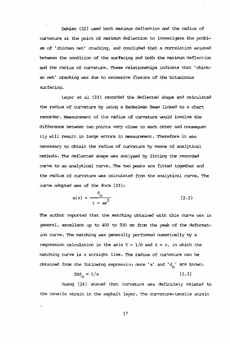
Leger et al ( 23 ) recorded the deflected shape and calculated

the radius of curvature by using a Benk.elman Beam linked to a chart

recorder. Measurement of the radius of curvature would involve the

difference between two p:>ints very close to each other and consequen

Uy will result in large errors in measurement. Therefore it was

necessary to obtain the radius of curvature by means of analytical

methods. The deflected shape was analyzed by fitting the recorded

curve to an analytical curve •. The two peaks are fitted together and

the radius of curvature was calculated fran the analytical curve. The

curve adopted was of the form (23):

d a(x) = 0

2 1 + ax

(2.2)

The author reported that the matching obtained with this curve was in

general, excellent up to 400 to 500 rrm fran the peak of the deformat-

ion curve. The matching was generally performed numerically by a

regression calculation in the axis Y = 1/d and X = x, in which the

matching curve is a straight line. The radius of curvature can be

obtained fran the following express inn once 1 a 1 and

2Rd = 1/a 0

Id I 0

are known:

(2. 3)

Huang (24) stated that curvature was definitely related to

the tensil8 strain in the asphalt layer. The curvature-tensile strain

17

ratio depends primarily on the thickness of the surfacing and was

independent of the road base thickness. The use of curvature, instead

of deflection, as a criterion for a:mtrolling fatigue, was highly

desirable because the curvature-tensile strain ratio was not affected

by m:xlular ratios.

The rrajor difficult'.! with the use of all these methods is

tl1at speed of operation; While suitable for short failure investigat­

ion . the Deflection Beam does not provide sufficient route capacity

for routine testing.

2.3.2 Deflectograph.

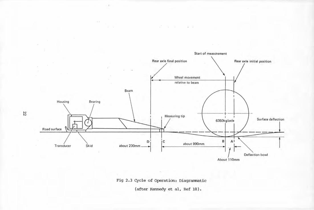
The Deflectograph, originally designed by the Laboratoire des

Pants et Chaussees in France (25), operates within the Wheel base of a

standard rigid Wheel base lorry. The principle of the pivoted beams

supported by a datum frame is similar to that of the Deflection Beam.

Two beams, one in each wheel path, are rrounted on a T-shaped datum

frame, Which rests on the road surface at its extremities. The two

beams, see Plate 2 .1, are attached through bearings to the recording

heads. During the measuring cycle the beams and the datum frame are

stationary on the road surface. The tips of the measuring anns are

t-J1en at a p::>sition approximately 1100 rnn ahead of the centreline of

the rear axle, see Fig 2.3. At this p::>int a switch is activated that

energises a solenoid within the recording heads, Which in turn causes

two anvils to grip a vertical spring attached to the core or armature

of a displacement transducer, see Plate 2. 2 ( 18) • The operation of

these anvils links the measurement ann and the transducer through the

beam ann extension. The tips of the measurement ann are, by then,

approximately 990 rrm in front of the centreline of the rear axle and

18

it is fran this r::oint, B in Fig 2.3, t."lat the measurement of deflect­

ion begins.

The downward !IOVement is detected by tb.e .measuring arms and

is transferred to tb.e displacement transducer via tb.e extension arm and

tb.e clamping solenoi<l. The output fran tb.e transducer is fed to the

analogue and digital recording equipment housed in the rear cabin on

tb.e. vehicle. When tb.e centreline of the twin rear Wheels has reached a

r::oint, D in Fig 2.3, 230 rnn in front of tb.e tip of the measurement

arms, tb.e clamping solenoids are de-energised; this allows tb.e transd­

ucer' s armature and vertical spring to fall back to tb.eir rest or zero

r::osition. After tb.e ll'la}l'lint.m deflection has been recorded, tb.e datLnn

frame and deflection beams are pulled fon.e.rd on steel skids at twice

t."le speed of tb.e lorry by a cable system, operated tb.rough an electro­

mechanical clutch, to tb.e next measuring r::oint. The measurements are

taken at approximately 4 m intervals.

The vehicle speed is arout 2 to 2.5 Km/hr giving a ll'la}l'linum

surveyed lengtb. of al::out 10 to 16 Km, providing al::out 2, 500 to 4, 000

readings per day in each Wheel patb.. The deflection measured by tb.e

Deflectograph is recorded relative to tb.e datum provided by tb.e

T-frame. The Deflectograph assembly, shown in Figs 2. 3, 2. 4 and 2. 5,

indicates tb.at all tb.e supports of tb.e T-frame will be affected by the

loaded Wheels during the measuring cycle and that tb.e front Wheel will

play a greater part in influencing tb.e measured values tb.an in tb.e

case of tb.e operation of tb.e Deflection Beam.

The canplex relation between absolute and tTIP..asured deflection

resulting fran the datum frame rotation is a major drawback of the

Deflectograph system. A further difficulty with tb.is approach is the

slow loading speed and tb.e difficulty this prQ~uces in selecting

19

appropriate layer rroduli which ccrnplicates any ccmparison between

measured deflections and those predicted by theory although in princ-

iple, this is possible if suitable layer rroduli are selected (26).

Guide roller

Plate 2.1 Oeflectograph-Beam Assembly

(after Kennedy et al Re£ 18).

T-frame

Beam

Point of measurement

The Oeflectograph has been m:x3ified by the TRRL to record the

deflected shape of the flCiVement' s surface as a maxinn.Jn deflection and

ten ordinate deflections, i.e. a multi value curvature rreasurement, see

Figs 2.6 and 2 . 7. The curvature of the pavement's surface is expressed

as a differential deflection, which in turn gives an indication of the

a:::li'ldition of the flCiVernent structure.

20

Differential deflection is the difference between the maximum

deflection and an ordinate deflection and is specifien in terms of the

horizontal distance between the two p:>ints of rreasurement, i.e. the

differential deflection 50 rrm £ran the maximum deflection relates to

the shFtpe of the. deflection dish over that distance.

2 • 3 • 2 .1 Pavement EValuation •

Butler et al (13) carried out theoretical studies, using a

two dimensional finite element approach, and practical studies, using

in-situ rreasurements of maximum deflection and deflected shape

obtained with a Deflectograph on a wide range of pavement types. The

finite element rrodel was used to detennine the relationship between

the deflected shape of the pavement surface and the thickness of the

bituminous layer. Charts (13) •...ere produced which enabled the p:>sition

of the differential deflection most influenced by a change in bitumin-

ous layer thickness to be identified and it was found to corresp:>nd to

an offset 200 rrm fran the p:>int of maximum deflP.ction. It was found

that the stiffness of the bituminous layer has a greater influence on

the deflected shape (differential deflection) than on the maximum

deflection, whereas the opposite is true for the rrodulus of the

subgrade. The differential deflection was less influenced by the

stiffness of the subgrade and the stiffness and thickness of the

granular layers.

The rrein draw back wit..'l the use of the Deflectograph for

analysing the resp:>nse of a pavement is the limitation of its current

-2 accuracies of measurements; 1 to 2 x 10 rrm. To be effective accur-

acies of 1 to 2 x 10-3 rrm are required.

21

Housing Bearing

Road surface

Transducer Skid

Beam

Start of measurement

' .-R-ea_r ... a,_x_l_e_f-in_a_l_p_o_si-tt_· o_n _______ \ ___ -+--~/Rear axle initial position

,.. Wheel movement

relative to beam

-+-----+ --+----+ Surface deflection

I

6350kg/axle

Measuring tip

I o'

about 230mm --1 c about 990mm

Fig 2.3 cycle of Operation: Diagrammatic

(after Kennedy et al, Ref 18).

AI

;!-Deflection bowl

f

About 110mm

Beam extension

Beam pivot .

Bearing housing------!.~~

Neg. no. A3153n1/8

Plate 2.2 Deflectograph-Rea:>rding Head

(after Kennedy et al, Ref 18) •

+----

Dimension Satisfactory range (mm)

F 990 ± 20 G 220- 230 H 1530 :t 5 J 1400 t 1 K 2130 ± 5

cb cp

Oamping / solenoid

Vertical spring

Displacement transducer

Fig 2.4 Di agranmatic Representation of Def1ectograph

(after Kennedy et al, Ref 18 ) •

23

c Wheel base and trade width

E

~~ ..... ~5 ...... ~a T 'f"k-Aa.,. __

--- -]· I • . ~---\-. l Contact area of tyre---{ )-----'-on road surface \ ______ _/

Dimensions and tyre contact area on one pair of rear wheels

Detail

Dimension A Dimension B Dimension C Dimension D Dimension E Front axle load Rear axle load Twin rear wheel load Tyres Tyre pressure

Satisfactory range

290-JBOmm 130-190mm 1830-1875mm 1980-2013mm 4445-4510mm 4500kg: 5% 6350kg: 10% 3175kg =. 10% 12.00 X 20 690kN/m2 (100psi)

0

Front axle

Fig 2.5 Essential Chassis Details Ear Deflectograph Vehicles

(after Kennedy et al Ref 18 ) •

24

undist\U"bed pavement surface

maximum deflection

--------------- ~en ordinate ce~ion measurements - . -,-

deflected shape

Fig 2.6 Recording the Deflected Shape as a Maxiroun Deflection

Undisturbed pavement surface

Maximum Deflection

Deflected Shape

and Ten Ordinate Deflection.

Horizontal Distance (L)

Ordinate

Differential Deflection

Fig 2. 7 The Relationship Between the Maxi.Inun, Ordinate

and Differential Deflections.

25

2.3.3 Travelling Deflectameter.

The Oeflectameter ( 16) consists of automated versions of the

Deflection Beam with the beams llDunted in front of each pair of dual

rear wheels of a 15 m long articulated lorry. It is longer and less

manoeuvrable than the Deflectograph (16). The beams are carried on a

large datum frame which stands stationary on the road, independent of

the continuously llDving lorry while the deflection generated by the

approaching wheel is detected and recorded. The datum frame and beams

are then carried rapidly forv.ard relative to the lorry, ready to begin

the next cycle of measurement. The lorries operate at 1 to 1 • 5 Klil/hr

and taking measurements at 6 and 11 m intervals respectively. The

capacity of this system is al::out 2,000 measurements per day. This

equipment is in use in california and Denmark and is capable of recor­

ding both the maximum deflection and deflected shape of the ·road

surface (16).

2. 3. 3 .1 P':lvement Evaluation.

The radius of curvature (R) of tl1e road surface at the point

of maximum deflection (d) or the product of 'Rd' can sanetimes be·

determined from the influence line, i.e. the deflection recorded as

the wheel approach!=s (27). Since the radius of curvature is difficult

to measure, an influence length is sanetime calculated as a measure of

the shape of the influence line. In Denmark, the length of deflection

curve is determined as the distance between two points at which defle­

ction is approximately 95% and 5% respectively of the maximum (27).

26

2.3.4 Curvature Meter.

The Curvature Meter ( 21, 28) y,as used in S .Africa to measure

the deflected shape and is based en the principle that the differen-

tial deflection occurring over ~ short distance is r e lated to the

curvature of the surface over that distance. The instrument, Fig 2.8,

a::nsists essentially of a short bar resting en the road surface at

toth ends with a dial gauge m:mnted centrally between the feet with

its .spindle in oontact with the surface. The instrument is placed 5 ft

(1525 rnn) ahead of the dual rear wheels of a loaded truck, in an

awroximatel y level p::>si tion. The truck is driven fon.erd slowly,

without stowing at any p::>int, and the maximum reading is reoorded as

the wheels pass directly q:p::>site the instrument (p::>int B in Fig 2.8).

'!'l.o negative maxima will also be observed 1 oorre Sp::>nd ing to p::>ints A

aro c. A final reading is taken when the wheels have passed 10 ft

(3050 mn) beycod the instrument.

:1aximum Deflection

s

I< L

/ 7 /

Positive Curvat ure

s

Fig 2. 8 The Curvature Meter (after Dehlen I Ref 21 ) •

The relation between curvature and dif ferential deflectien

may be deduced by simple geanetry, by fitting an approximate curve to

the three p::>ints of measurement: the maxirnun and two p::>ints of

27

inflection. Previous work (21) undertaken in S.Africa with a Benkel.Iran

Beam has indicated that in the vicinity of the p::>int of maximun defle-

ction, the deflected shape is typically a sine form. It has also been

ooted that p::>ints of inflection ( tnints P in Fig 2. 8, where the curve

changes fran concave to convex) occur fairly consistently at distances

of 6 inches (153 rnn) on either side of the p::>int of maximun deflect-

ion. The relationship betvJeen the curvature and differential deflect-

ion in the case of a sine curve is ( 21 ) :

(2.4)

where L = distance between the dial gauge and each supp::>rt,

Dd= differential deflection,

f = factor ....nich varies between 2.0 and 2.47 as the ratio L/ S

varies between 0 and 1.

L L

sha!?e of e road's surface

I

Fig 2. 9 Recording Curvature w:i th a Curvature Meter

(after Dehlen, Ref 21 ) •

The Curvature Meter is tmable to J'T'easure the total deflect-

ion occurring beneath the wheels and a telescope or a pair of binocul-

ars is needed to read the dial gauge, ....nile sitting on the road behind

28

the vehicle • Use of this equipment in the U.K. has indicated that

'Dd' has a range of 0.001 to 0.002 inches 011 !IDtor.'ldys, and up to

0.015 inches 011 roads of light construction.

2.3.4.1 Pavement EValuation.

This instrument was developed to carry out the same task as

that of the Benk.elman Beam. The evaluation process is the same as that

. _ described in Section 2 • 2. l . l.

2. 4 Stationary LOading Techinques.

Stationary Loading techniques cover a wide range of loading

conditions including static loading of the Plate Bearing Test and two

forms of dynamic loading ....tlich apply either steady state sinuso-1dally

varying force of a single impulse transient force, to the pavement

surface. The pavement is loaded by a pulse of constant duration

irrespective of depth and the planes of principle stress do not

rotate, Dynamic deflection is represented by a curve, indicating pave­

ment reaction, with the amplitude of the deflection expressed in terms

of the frequency of application of the load • A particular deflection

value can be determined for a given frequency fran the curve. Stress­

strain conditions generated by these tests are not representative of

conditions in the pavement structure under nonnal loading conditions

and the deflection response of frequency and stress dependent mater­

ials will be affected.

29

2.4.1 Plate Bearing Test.

The Plate Bearing test consists of an allrost static load

applied to a circular loading plate. The pavement is usually subjected

to a number of load cycles before the reoound deflection is measured.

There are several test methods and the results obtained depend on the

equipment used, load, duration of the load application, stiffness and

diameter of the plate and the location of the measuring devices.

Repeated static Plate Bearing Tests to determine pavement

layers properties (estimate of layer m::x'luli) and deflection are cnmo­

nly used in Denmark and Finland (27). The test is slow and in general

is not accurate. The speed of operation limits the number of test

results that can be obtained, usually about 2 to 10 measurements per

day, and these are usually insufficient to asse~the homogeneity of

the pavement with distance.

2.4.l.l l?ave:nent EValuation.

It is possible to:

(a) measure the deflection under a given load;

(b) measur~ the load corresponding to a given deflection;

(c) determine the elastic deformation m::x'lulus corresponding to a

pressure/deformation curve;

(d) detennine the m::x'lulus of. each layer of a 2 layer system by using

several loads with plates of two or three different diameters.

The deflection is measured through the centre of the plate. The

repeated rebound deflection is used for calculation of E-values.

30

2 .4. 2 The Falling weight Deflectaneter.

The Falling Weight Deflectaneter equipl!E!lt (27) applies a

pulse load by dropping a weight of 150 Kg onto a set spring system

which in turn transmits a load pulse of atout 28 ms duration to the

ro'l.d surface by means. of a circular plate of 300 rrm diameter. The

maximum force developed is 60 KN When dropped fran 400 rrm high. The

deflection of the pavement is measured by means of velocity transd-

ucers, one in the centre of the loaded area and up to 5 transducers i'it

a fixed distance fran the load. 'l'his enables the shape of the deflec-

tion towl to be characterized. The equipnent is carried on a single

axle trailer tov.ed by a vehicle carrying the p::>wer supply and record-

ing equipnent. The towing vehicle also houses the =ntrols for the

loading cycle and for the operation of the hydraulic jack, used to

raise the trailer When a test is being carried out. Maximum output is

of the order of 200 measurements per day.

The equipment does not measure the absolute deflections,

because of the seating load, but a datum is fixed. Repeat measure-

ments are required because of the single load pulse method of testing.

The pattern of load pulse developed within the structure differs fran

that developed under traffic in that its duration is independent of

depth and principal stresses do not rotate.

A parameter, 1 Q 1, is used to define the ratio of the

r

deflection (d ) at a distance 1 r 1 fran the load to the deflection r

under the cent-.re 1.)f the test load (d0

). Claessan et al (29) stated

that "the parameter 1Q 1 vas choosen instead of the radius of curva­r

ture, because 1 Q 1 can be measured llDre easily and provides equival­

r

ent information". For typical structures, 1 r 1 has been fixed at a

distance of 600 r.m and the curvature expressed as tht~ a500 Btio.

31

2.4.2.1 Pavement Evatuation.

Using the BISAR ccmputer program (30), graphs such as that

reproduced as Fig 2.10 (29) have been prepared giving the relationship

bety,een E1

(rrr:x:lulus of the asphalt layer), d0

, Qr and H1

(thickness of the asphalt layer) for predetennined values of E2

(rrr:x:lulus of untound or cemented base layer), a2

(thickness of base

layers), E3

(rrr:x:lulus of the subgrade) and the distance r, for a

given test load. Fran such graphs, with d and Q measured, two o r

unknown structural parameters can be detennined if the other variables

are known or can be estimated.

In the studies carried out by Van der Poel (31), the deflect-

ion is calculated at three points of the pavement surface, one at the

centre of the loaded area ( d ) , one at a distance of 600 mn of the 0

centre ( d600

) and one at a distance of 2000 mn ( d2000

) • The shape

of the deflection l::owl is characterised by the surface curvature index

(SCI), calculated by subtracting d600

fran d0

• In relation to the

maximum deflection ( d0

), the SCI value gives an indication of the

pavement properties, while d2000

am be related to the bearing capa­

city of the subgrade. As described in Ref (31) the rrr:x:lulus of the

subgrade can be calculated fran the deflection, d , measured at a r

distance, r, fran a loaded area with a contact stress, q, and a radius

of 'a':

E = r

where p. = Poisson' s ratio.

(2 .s)

The major restriction to the use of this fonn of equipment

for pavement evaluation is the strong dependence of predicted pavement

material properties on the measurement of maximum deflection and

32

deflected shape; information on the repeat ibility of the rreasur~

ments has not been published.

1011

I

6

2

10

I

6

2

6

E,, N / m2

Q 600" 0 60018 0

Hz •300mm

E2 •2 .7xE 3 E3 • 100MN/m2

p •10000 N

o •150 mm

JL-. •!kz ·~. 0 35

~Lo----~2--~~.~_.6~1~1~oy----2._~~·._.-6~~~~1o3 80

, 10-6m

Fig 2 .10 Deflection Interpretation Chart

(after Claessen et al, Ref 29 ) •

2 .4.3 nynaflect.

The Dynaflect ( 32) is an electranechani.cal system for rreasur-

ing the dynamic deflection on the road' s surface caused by oscillatory

load. Measurements are independent of a fixed surface reference. It

cc::nsists of a small, tv.o Wheeled , trailer, carrying a dynamic sinuscr

idal force generator in the form of tv.o oontro-rotating masses. The

dynamic force varies at a fixed frequency of 8 Hz with a maximun value

33

of '227 N, Which is superi.mp:>sed on a static load of 725 Kg and is

transmitted to the road surface through the two small rigid Wheels

located 0.5 m apart. The maximum deflection is recorded midv.ey between

the Wheels together with the deflection at four other r:oints along the

centre line, between the Wheels, spaced in the longitudinal direction

<~t 305 mn intervals. Deflections are measured with velocity sensitive

transducers and are recorded by equipnent carried in the towing

vehicle. The deflection basin parameters associated with the oynaflect

measurement are shown in Fig 2 • .ll. 'I'he five parameters associated with

each Dynaflect measurement are described ':'IS follO\VS (32):

(a) Dynaflect MaJCimum Deflection (DMD)

(b) Surface CUrVature Index (SCI)

(c) Base CUrVature Index ( B:I)

= w1

(1st sensor deflect­

ion); measure of pavement

structural characteristics

and support condition.

= w1

- w2

(differential

deflection between the 1st

a~d 2nd sensors); an indica-

tor of the structural condi-

tion of the surface layP-r.

= \'V4 - w5 (differential

deflection between the 4th

and 5th sensor) ; measure the

base supr:ort conditions.

(d) Spreadability (SP%), [100(W1

+ w2

+ w3

+ W4

+ W5

)J

swl

= (average deflection as a

percentage of the lMXimum);

measure the load carrying

34

(e) Fifth Sensor Deflection (w5

)

Orioinal surface

----...... .........

" ' ' ' \ \ \

' 11'1

capacity and stiffness ratio

of the pavement structure.

= w5

; indirect measure

of subgrade rn::Xlulus.

Wmoa s O)'nofteet maalmum deflection (numerical value ot sensor •t SCI • Surface curvature lnd•• (num•ricol difference of sensor MI and .41 21 BCI • Base curvature indtl (numerical difference of sensor .r:4 and •s) SP% • Wt+W2+WJ+W4+Ws • 100

5 w, W5 = Num•ricat ... atut ot sensor • 5

Fig 2 .11 Dyna£lect Deflection Basin Parameters

(after Bandyopadhyay, Ref 32 ) •

2.4.3.1 Pavement Evaluation.

Studies of pavement condition evaluation fran Dynaflect

deflection basin parameters have been carried out by several authors

(15, 32, 33) and several conclusions have been deduced fran their

work. CMD is a measure of pavement structure characteristic and

support conditions.

SCI is predan.i..na.ntly an indicator of the structural condition

of the surface layer. SCI is inversely prop:>rtional to the radius of

35

curvature and is therefore a measure of tensile strains in the pave­

ment. Majidzadeh (15) sho..ed that SCI is dependent on pavement thick­

ness and the m::x:'lular ratio E/E2

(pavement m::x:'lulus/support

m::x:'lulus) using a two layer elastic m::x:'lel. For a relatively thick pave­

ment, SCI decreases with an increase in the m::x:'lular ratio E/E2

,

whereas fOr a tl1in pavement, the SCI-E1

/E2

relation depends great-

ly on the magnitude of thickness, H (pavement thickness), an increase

in tllickness reduces the SCI parameters. It was shown (15) that the

tensile strain at the rottan of the pavement layer and the vertical

strains on the subgrade are prop:>rtional to the SCI. It has been

rep:>rted (33) that the SCI parameters could be used for detection of

problem areas in the pavement layer. The adequacy of load transfer at

joints, effect of transverse crack planes and roads containing concre­

te quality have been evaluated in numerous pavements in Ohio (u.s.A.)

using the SCI parameter. This parameter can be used to detail areas of

deficiency at tlle pavement surface layer.

The BCI has been widely used as a parameter suitable for

detection of problems in the subgrade and the base layers. BCI values

ranging from 0.05 to 0.11 are generally representative· of satisfact­

ory performance, whereas p:>arly performing fldVements show BCI values

greateF than 0.1 c; t:n (). 2.

w5

has been shown (33) to be an indirect measure of sub­

grade m::x:'lulus and is relatively insensitive to pavement ~1ickness and

m::x:'lulus of surface layer.

The SP% describes the slab action of the p<!.Vesnent and its

ability to distribute load. Pavements with high SP% values Cl istr ibute

loads rrore effectively and the resulting stresses and strains on the

suhgrade are smaller. The ability of tlle pavement to absorb the

36

indLCed stresses is reflected in the spreadibility parameter, which,

in turn, is a function of pavenent thickness (H), nodular ratio,

E/E2

(paverrent rrodulus/ Supp:Jrt nodulus), and other geanetrical

variables. It was sh()<M'l (33) that a higher SP% is not al....ays a guara-

ntee for satisfactory pavement performance, especially for thin pave-

ment where the effectiveness of load distribution decreases with a

decrease in paverrent thickness. A structural diagnosis chart based on

Dyna£lect deflection parameters, prepared by Bandyopadhyay ( 32) , is

sl'o.Yn in Table 2 .1 •

The main drawback of this system is that the low force level

does not represent lorry traffic and a fixed frequency of 8 Hz sane-

times proouces resonance. The equipnent can therefore be used to id en-

tify fOssible VJeak areas but the estimation of material properties

~ the results must be questionable.

0110 SCI BCI CONDITION OF PAVEMENT STRUCTURE.

CHECK EACH EVALUATION WITH sP•t. AND Ws CRITERIA

G.T. 0.12 PAVEMENT AND SUBGRAOE WEAK G.T. 0.16

LE. 0 . 12 SUBGRAOE STRONG, PAVEMENT WEAK G.T. 1.40

G.T. 0.12 SUBGRAOE WEAK, PAVEMENT MARGINAL L.E. 0 . 16

L.E. 0.12 OMO HIGH, STRUCTURE OK

G.T. 0 .12 STRUCTURE MARGINAL, OMO OK G.T. 0 . 16

L .E:. 0.12 PAVEMENT WEAK, OMO OK LE. 1.40

LE. 0 . 16 G.T. 0 . 12 SUBGRAOE WEAK, OMO OK

L.E. 0.12 PAVEMENT AND SUBGRAOE STRONG

Table 2 .1 Structural Diagnosis Chart Based on Dynaflect

Deflections (after Bandyopadhyay, Ref 32) •

37

1.4.4 Road Rater.

The Road Rater (34) is pov.ered fran an electro-hydraulic

power unit attached to a van or truck. It serves as a means of measur­

ing a road 1 s strength by the application of a dynamic load of 445 N,

operating at frequencies between 10 and 50 Hz superimposed on a static

load of 500 Kg. The road 1 s deflection profile, measured by four veloc­

ity sensors housed on a l:xx:.rn and spaced 0.35 m apart, is displayed

visually on instrumentation located inside the vehicle. About 300

measurements at a single frequency or alternatively 100 at 3 frequency

are possible in a working day. The actual· number is dependent on the

spacing of the points of measurement. This equipnent is used in the

u.s.A. and in Italy (16).

Kilareki et al ( 35 ) , used the Road Rater deflection basin to

calculate the Surface CUrvature Index (SCI), the Base CUrvature Index

(OCI) and the Base Damage Index (BDI). These criteria were correlated

with the maximum tensile strain, the fatigue cracking of the pavement

sections and traffic loading; a relationship was established between

the SCI and the traffic loading resulting in the prediction of remain­

ing pavement life.

The main drawback is similar to that of the Dynaflect in that

unrealistically small loads are applied in relation to those applied

by lorry traffic.

2.4.4.1 Pavement Evaluation.

Using the BISAR a:rnputer program (30), the deflection values

corresponding to the asswned rrcx:lulus values are a:rnputed (34). The

calculated deflections are then a:rnpared with the measured deflections

and the assumed rrcx:lulus valuP-s are corrected. The correction begins

38

from the subgrade nodulus and proceeds sucessively to sub-base, base

and surface noduli. This iteration process is repe'ited until the

difference between the calculated and the measured deflection~ 5)r the

four sensors are within the specified tolerance. In the theoretical

developnent of the nodulus evaluation procedure, it was shown that the

deflection at the £ourth sensor is essentially dependent on the

subgrade modulus only, Whereas, the deflection at the third sensor can

be approximated with sufficient degree of accuracy as a function of

only the moduli of sub-base and subgrade. The following relationship

were suggested ( 34) :

-1.04 E

4 = 67.88 x 5

4

E3

= 1492.85 x 83- 7 •26 x 8

46 •24

Where E4

= 8ubgrade nodulus l.I1 105 lbf/ in2

,

E3

= Sub-base nodulus in 105

lbf/ in2

,

8 = Deflection at fourth sensor in 10-6 in, 4

83

= Deflection at third sensor in 10-6 in.

(2.6)

(2.7)

It was reported (34) that the modulus values of surface, base

and subgrade will be greater and those of the sub-base will be lo...er

When evaluated fran ROad Rater deflections canpared to those determin-

ed fran repeated load and plate load tests. The discrepancy in the

nodulus values could be due to the effects of dynamic loading and

stress (or strain) level effects. Plate load test is a static test and

the repeated load test can also be considered as a static load test

because of its loading frequency (20 cycles/min) When canpared with

the Road Rater loading with a frequency of 25 Rz or 1500 cycles/min.

'I'he stress level in the pavement induced by the Road Rater is cxmside-

rably lo...er than those generated by the plate load. Therefore, under

the low confining pressure, the sub-base l!E.terial will exhibit a

39

smaller m:::>dulus. At a deeper level, the low deviator stress level

induced by the Road Rater results in a significantly higher subgrade

m:::>dulus canpared to those detennined fran plate load and repeated load

test. Therefore the a:mbined effects of dynamic loading and low stress

intensity yield higher m:::>dulus values for the subgrade and lower

m:::>dulus values for the sub-base material when canpared with the

m:::>dulus values detennined fran the laboratory repeated load tests and

field plate load tests.

Kilareski et ~1 (35) reported that the surface deflection at

geophone No.l, d1

(located at tJ1e centre between the loading plate),

is rrore sensitive to the variation of tJ1e ,:;llrence m:::>dulus, E1 , than

d2

. 80th d3

and d4

are insensitive to the variation of the

i!"Cdulus ;::1

• A similar effect was observed with the variation of the

base m:::>dulus , E2

as that of E1

• The sub-base m:::>dulus E3

, signif­

icantly affects. all deflection values except for d4

(geophone

deflection No 4). All four deflection values decrease considerably

with an increase in the subgrade m:::>dulus E4

• The BISAR canp.lter

program ( 30) , was used to analyse ~ four layer elastic system, and the

deflection values d1

, d2

, d3

and d4

corresponding to the

assumecl values of i!"Cduli v..ere calculated (34). These calcul~ted o~fle­

ctions are canpared with deflections measured at the four geophones.

Ne\v assumed m:::>dulus values based on the previous values v..ere calcula­

ted using the equat_ion stated in Ref (35). The iteration process is

repeated until the difference betv..een the calculated and measured

deflection for all sensors are within ~ specified tolerance.

40

2. 5 wave Propogation Technique.

The structural condition of the pavements can also be assess­

ed by measuring the velocity of propagation and length of waves pro_[X>­

gating fran an applied dynamic loac (36). Steady state loading is

nonnally used. High frequency produces a short wave length surface or

Rayleigh waves, which travel at speeds determined by the surface layer.

At lrn..er frequency, wavelengths several times that of the structure

are produced and these characterise the lower layers of the pavement

and the subgrade.

2.5.1 Pavement EValuation.

The stiffness of the surfacing and subgrade layers can be

determined by extrapolating parts of the dispersion curve (plot show­

ing the relation between phase velocity = frequency x wavelength, and

wavelength) to zero wavelength. Interpretation of the remainder of the

dispersion curve can only be achieved by the o:::mparison with the

the.ortical curves based on the theory of elasticity. Using the Wave

Propagation techniques it is only possible to cover two sites per day.

The main drawback of the method is therefore that it is very slow. In

addition, the stress level imposed by these tech n i.ques is small and

the pavement stiffness obtained will therefore, differ fran that

generated under moving traffic loads.

2.6 Factors Affecting the Selection of Pavement EValuation Equipment.

The following factors must be considered before undertaking

any structural strength measuring equipment:

(a) General Requirement.

( i) the total distance and range of environmental conditions of

41

the site;

( ii) the purp:>se of the investigation failure or routine

structural strength survey;.

(iii) the range of ccnstruction and material type to be tested;

(iv) availability of suitable skilled staff to operate the

equipment and to analyse and interpret the data.

(b). Equipment Requirements.

( i) suitability for daily and yearly route capacity;

(ii) ability to test a wide range of oonstruction and material

types;

( iii) provision of a rapi<:] system for processing and assesing the

collected data;

(iv) should be linked to an authoritative design method.

For the output of the method to be effective in designing

streng.th·.ening measures, it is i.mp:>rtant that the measurement input to

any design method is sufficient.

2. 7 Justification for the Selection of Deflectograph.

Research carried out over a number of years at the TRRL, has

established that a significant relation exists between the magnitude

of the deflection of a road pavement under a rolling wheel !TDving at

creep speed and the structural performance of that road • Under traff­

ic, systematic measurements of deflection obtained on toth orginal and

overlaid pavements has provided the basis for prediction of the unexp­

ired lives of pavements and for the design of bituminous overlays to

extend their lives.

42

In selecting a .method of rne3.surement, the TRRL opted for the

realism of the rolling wheel and given the empirical approach orginal­

ly planned, accepted the Deflection Beam for development into a stand­

ard measurement technique. However, extended surveys over long lengths

of llDt.Orway and tnmk road, denonstrated the need for a measurement

techniques of greater capacity than that provided by the Deflection

Beam, which testing at 10 m intervals, can cover only 1 Km of road in

a ....orking day.

The TRRL therefore purchased the Deflectograph which carries

out measurement of deflection at closely spaced intervals and it is

fOSSible to survey 8 to 10 Km in a working day. Despite the drawbacks

given in Section 2.3.2, its use for measuring curvature has been

investigated because:

(a) It is used extensively for monitoring highway net....orks;

(b) It has the greatest_route capacity and the ability to take measur­

ement at short intervals a:::rnpared to the other equipment;

(c) The performance aspect of existing design method is accepted;

(d) If the curvature information could also be obtained and interpret­

ed, it ....ould give a very p:>....erful evaluation system.

43

aiAPI'ER 3 .0 MATERIAL rnARACI'ERIZATION FOR FLEXIBLE PAVEMENT DESIGN.

3 .1 Intrcx:l uction .

In the design of a road pavement there are two aspects of

material properties which have to be considered. Firstly, the load­

deformation or the stress-strain characteristics of the material used

in the various layers of the structure need to be known so that analy­

sis of the stresses and strains at the critical p::>ints can be perfonn­

ed. secondly, information is required on the likely rrode of failure of

the various materials under repeated application of load so that the

design criteria in the form of maximum allowable stresses or strains

can be incorporated into a design procedure. The ·material used in the

flexible pavement construction fall essentially into four categories,

bi twninous round, cement round, unbound aggregate and cohesive

subgrade soil. Non-cohesive material can be classified as unround

aggregate. All these materinls are non-hanogenous, anisotropic, non­

linear and generally non-elastic.

Pavement performance does not depend solely on the charactis­

tic of the materials in the individual layers but rather on the inter­

action of the various layers. This interaction of the layers will

itself depend on the thickness of the layers as well as the material

characteristics.

3.2 Bitt.nninous ~laterials.

Bitt.nninous material is mineral nggregate mixed with either

tar or bitwnen or with one of the low viscosity cut back bitwnen or

bitwnen enulsion binders. Traditionally in the U.K., bitt.nninous road

44

materials can be clnssified under three basic mixes types which are:

(a) Hot Rolled Asphalt (BS594, Re£ 37);

(b) Dense Bitumen (or tar) Macadam ( BS4987 , Re£ 38 ) ;

(c) Open Textured Macadam ( BS4987, Ref 38) •

3.2.1 Hot Rolled Asphalt (HRA, Re£ 37).

This is a gap graded material including. filler and a relativ­

ely hard grade of bitumen. The bitumeri content is high and the mechan­

ical properties of the material are influenced primarily by those of

the bitumen sand-filler llDrtar. The a:>arse aggregate bulks the mixture

and contributes to its stability. Fine aggregates fonns the major

proJ:X)rtion of the I!Ortar while the filler stiffens and strengthens the

binder. Bitumen binds the whole mi.xture together and provides. water

proofing. Canpacted rolled asphalt mi.xes are dense and basically

impervious from the time of laying and J:X)ssess good load spreading

properties and durability. HRA is extensively used £or ·the wearing

course, on heavily trafficked roads, but can also be used for the base

course and the roadbase. It is easy to canpact and therefore relative­

ly insensitive to site conditions and quality of technical supervis-

3. 2. 2 Dense Bitumen macadam (DBM, Ref 38).

This is a uniformly graded material often using a softer

binder than rolled asphalt. Its properties are partly influenced by

interparticle friction and interlock, which is the characteristic of a

macadam, and partly by the viscosity of the binder. The a:>arse aggre­

gate provides the main skeleton of the interlocked aggregate and prov­

ides the distribution of the traffic loads. Fine aggregate fills, or

45

partially fills the voids in the coarse aggregate skeleton and it has

a significant bearing on the finished surface texture. Filler increa­

ses the viscosity of the binder, thus reducing the risk of binder

draining fran the aggregate. Caribined with the binder, it helps to

fill small voids. Binder acts as a lubricant between the aggregate

particles particularly during canpaction and also as a water proofing

and l:x:lnding agent.

'!'he bitumen content is relatively low and this makes it a

cheaper material than rolled asphalt. These materials tend to be used

for the roadbase and the base course layers, though they may also be

used for surfacing ( 39) •

3 • 2. 3 Open Textured Macadam ( 38 ) .

This is a unifonnly graded material with low binder content.

It has a high void content when canpacted and therefore it is not useCl

as a major structural layer. The main function of its ingredients are

the same as those of DBM. It is used for surfacing minor roads and has

the advantage of providing a relatively dry surface under wet conditi­

ons. The ability of very open t.:;,xtured mixes to drain surface water

has been exploited for surfacing runways when the material is under­

laid by an impenneable layer.

3.3 Stiffness Characteristics.

Bituminous materials are viscoelastic and therefore e1eir

stress-strains characteristics are dependent on l:x:lth time of loading

(t) and temperature (T). Van der Poel (40) defined the stress-strain

relationship as the stiffness (S):

S (t, T) = Stress/TOtal Strain (3.1)

46

.. E z ;L

.D Vl

10)

102

10

X)'

102

10·)

The variaticn o f stiffness with time and temperature is sh<::IY.n in

Fig 3 . 1 for a typical bitumen stiffness. The mix stiffness depends on

the mix variables such as aggregate type , and grading, bitumen type

and content and degree of mix canpaction and the resulting air voids

content.

Elastic behavio.Jr. 5 = E

Visco - elastic behaviour

Viscous betxlviour 5=~

t

ti ... 10~ 10-i; 10 ... 10.1 10'

Time ( s l

Fig 3 . 1 Variaticn of Bitumen Stiffne.s s With Time and Temperature

(after Brown, Ref 40)

3. 3 . 1 Estimation of Bitumen and Mix Stiffness .

3.3 . 1.1 Bitumen Stiffness.

Bitumen stiffness varies with loading time and t~rature

exhibiting elastic behaviour at low temperature and short loading

time, viscous behaviour at high temperature and long loading time and

viscoelastic response in between . This i s illustrated clearly in

Fig 3 .1 • The stiffness of bitumen, ~, can be estimated with the aid

of a rx::rrograph, see Fig 3. 2, developed by Van der Poel ( 41 ) and which

requires the £allowing data:

47

(a) LOading time, t(sec) or frequency, f(Hz);

(b) Temperature, T(0c);

(c) SOftening Point (reoovered, SP ) fran the Ring and Ball Test, r

(d) Penetration Index, PI, which is a rreasure of temperature suscept

ibity.

The penetration index ( recnvered) is calculated using the following

equation (42):

Pir = 1951 - 500 log Pr- 20 SPr

50 log P r - SP r- 120 .1

(3.2)

If recovered binder properties are not available, then they can t:e

estimated fran the initial properties using the following equations

(41):

P = 0.65 P. r l.

SPr = 98.4- 26.4 log Pr

(3 .3)

(3 .4)

The loading time may t:e determined fran Fig 3.3, which requires an

estimate of the asphalt layer thichness (H mm) or alternatively the

following equation (42) may t:e used:

-4 ., log t = 5 X 10 H - 0. 2 - 0. 94 log V (3 .5)

As an alternative to using the namograph, the following equation (42)

may t:e used to calculate the binder stiffness:

~ = 1.157 X 10-7 X t-Q• 368 x 2.718-Pir X (SPr- T)S

(3 .6)

The ranges of applicability of this equation are as follows:

Pir = -1 to 1, (SP -T) = 20 to 60 °c, r

t = 0.01 to 0.1 sec, ~ = MPa

48

+7

+6

+~

)( +4

"' +3 '1J .5 +2 1o·• 10"' IO. z c +I 0 .,.,

·~ 0 n:l ~ ...

-I ~

~ "' c - 2 "' a.. -3

Stiffness modulus, N/m2

10' .. 101 ..

7 7'

L//

! - 3

I

- 2

Temperature difference, °C

_,

-10'

_.!.!1.

=

--b

10' i 2

-10

ooo » "' ~ 10 .10 eo .\ .n Above T 800 pen .. ,l,,t.LI.I.!.I ... J,,I,,.!.,,L,. L•, , 1

I

ro ., ., oo uo liO uo •eo .,., ..o •• ,., ,1,.,.1.., !. .. 11o o 110 I ,. ,L ol o .!. .,, ! .,,!.,11!.

Example:

... -1, 1 Below T 800 pen

The st.lffneu modulus, defined as the ratio 0 / E = stresa/straln, Is 1 function

of time of loading (frequency), temperature difference with T800 end PI pen' .

T 800 pen Is the temperature et which the penetration would be 800.

This Is obtained by extrapolating the experimental log penetration

venus temperature line to the penetration value 800.

At low temperatures end/or high frequencies the ttlffneu modulus

of all bltumensasymptotes to a limit of approx. 3 x 109 N/m2

Unlu:

1 N/m2 = 10 dyn/cm2 = 1.02 x 10·5 kgf/cm2 = 1.45 x 10..,.1b/sq. In.

1Ns/m2 =10P

I

I

I I

I I

I

r---- Frequency, Hz --+---10' IO' lOs oJ

Operating conditions

Temperature : 11 °c

Loading time : 0.02 teeonds

Characteristics of the bitumen In the mix

T BOO pen temperature at which the penetration

Is 800 0.1 mm : &4 °C

PI, penetration Index : 0

Connect 0.021 on time scale with temperature

difference 64- 11 °c on temperature scale.

Record n l ffneu on grid at PI = 0

The stllfntu of the bitumen determined with this nomograph Is

sblt = 2.0 x 108

Nt m2

Time of loading, s

Fig 3. 2 Narograph for Determining the Stiffness Mcx'}ulus of Bitwnens

(after Van der Peel, Ref 41).

Z•I01

0 ·5 O·L. 0 ·3

0 ·2

Vl - 0 ·1 w ~ 0 ·07

~ 0 ·05 o O·OL. <! 0 _J 0 ·03

0 ·02

0 ·01

~ -- r--- --------~ ------- -~ --I--

~ f..---f--- -- f-- f..--r- ----~ ~ f..--~

-r---,....-

--f.-------

----- --- -~ -~ -

,..,

1-2

3

< rn 0 ~

r rn (./)

0 \J rn rn 0

A" f-1.1 0 3 --::r

o2 1l. 0

0 -u·

10

0 100 200 300 L.OO 500 600 THICKNESS OF BITUMINOUS LAYER (mm}

Fig 3.3 wading Tilre as a Functico of Vehicle Speed and

Layer Thickness (after Brown et al, Ref 42) •

3.3.1.2 Mix Stiffness.

Van der Poel (40) has shown that the stiffness of a mix

(Sm) containing dense graded aggregate and bit~ is primarily

dependent co the aggregate. Heukelan and Klanp ( 43) extended the ....ork

of Van der Poel and deduced the following relationship for the mix

stiffness:

c = V

(3. 7)

vol of Agg

Vol of Agg + Vol of bit~

~ = stiffness of bitumen fran narograph in MN/m2

•

so

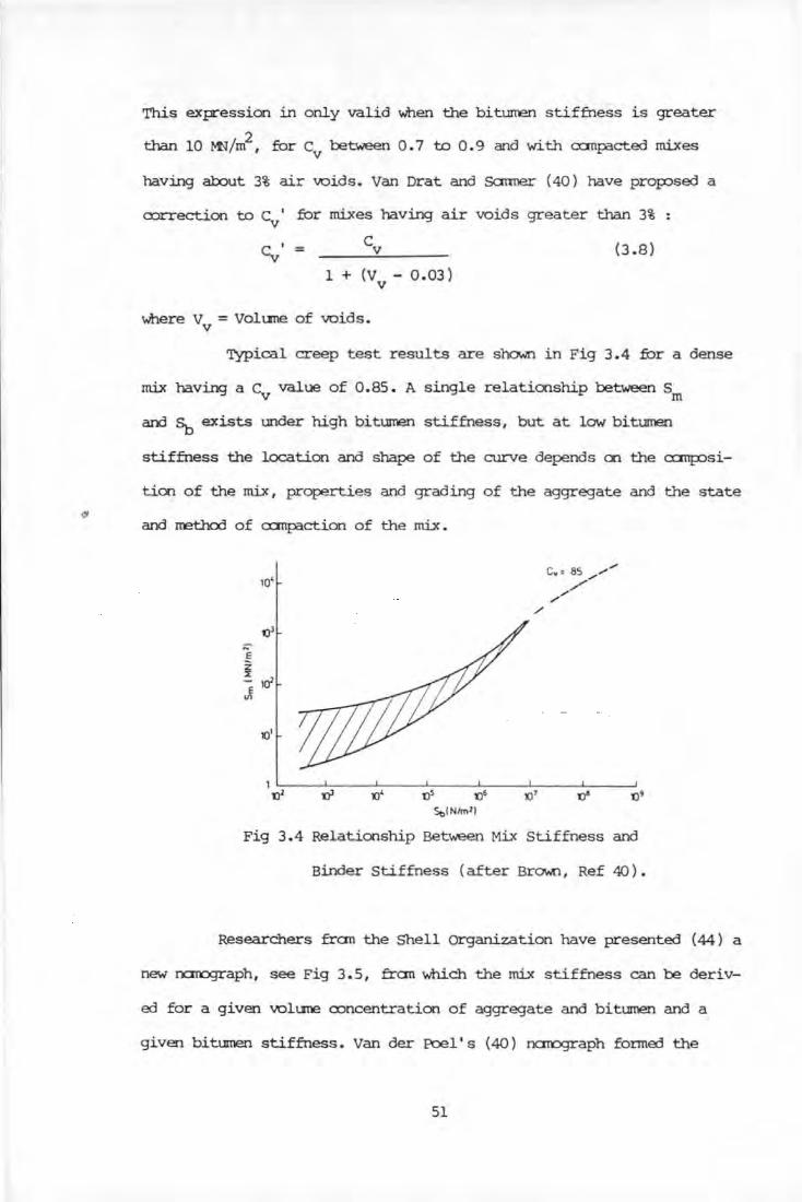
This expression in only valid ...men the bitumen stiffness is greater

than 10 l"N/m2 , for c betw'een 0. 7 to 0.9 and with a:mpacted mixes V

having about 3% air voids. Van Drat and Scrrrner (40) have profOsed a

oorrection to c ' for mixes having air voids greater than 3% V

Cy' = c V

1 + (V - 0.03) V

(3.8)

...mere V = Volume of voids. V

Typical creep test results are shown in Fig 3. 4 for a dense

mix having a c value of 0.85. A single relationship between s v m

and ~ exists rmder high bitumen stiffness, but at low bitumen

stiffness the location and shape of the curve depends on the ccmp:>si-

tion of the mix, properties and grading of the aggregate and the state

and m:!thod of a:mpaction of the mix.

10'

/

10'

St,IN/m2)

Fig 3.4 Relationship Between Mix Stiffness and

Binder Stiffness (after Brown, Ref 40) •

Researchers fran the Shell organization have presented (44) a

new ocm:::Jgraph, see Fig 3.5, fran which the mix stiffness can be deriv-

ed for a given volune concentration of aggregate and bitumen and a

given bitumen stiffness. Van der Poel' s ( 40) nc:rrograph formed the

51

basis for this new narograph.

80 90 ....... r--... .......... ......

70 '" "\... " f'.. Mineral

60.._ ~ !'\.. " ~ "' r\. aggregate,

' ' t\. ["\. """" "

.~ t'-,. l"

Stiffness modulus

of the bituminous mix,

N/m2

~ "' 0 /o v (V g)

' " ..... t\. ~ ~'-<: ~ ""-~---~-----40 '

20 ...... ...... 1'\. ...... ...... ...... ...... ...... 95

"' ..... "' " ["'\. " 0 " "' ' " "\..."t. "\... "\... ~ " ~ 0 "' .....

t\. "" "i ~ ~ "' I" ..... ' ' I~ c~ " "' ~ ~ ~ ["\. " "

Stiffness modulus ~ ~ "' "' ), '\. r--.. ~ r'\,. " " 85 of th e bituminous binder,

N/m2 ..... vb ...... " ...... ..... 1'\. "' ...... ......

I 0... ....._......_.

"' " " 100 40 30 20 10 5"' t'-.."'\.t ~ " " ""'" ~ '\ ~\ \ \ \\ ~ " i"-""

IS "' 75

2 " "'-\ '\. 1'\. \ ..... , ..... " ""'

"\... "\... " -

' r'\. \ \\ • """ ,~ ""' "r--.. 1"- " r'\,. 109 I 65 =

8 = 6 ...... '. \\ I ...... " ---"\ ~'\ ·" "' "' " ' 4

~' -

~ ~\ "~ ' "' 50 -~---·---~~ "' ~ " 2 ' t\. -

~ l\ "' ' -"\ "' ~ " 30

taB ~ ~ = 8 -

6 10 = ~~ -\'.'\: 4 r \\ ~ 80.5 ~~~:~·~ ~ '\. ~ 2 aggregate

\' '\. t\."\ ~

Jv.! ~· ~ ~ -I-

" 107 13.1 Bitumen 8 -'-

Air 6.4 6 0 /o v -"" '.

5 10 20 30 100

e.g. Stiffness modulus of the recovered Stiffness

binder 2 x 108 N/m2 > modulus Bituminous binder,

Volume of binder Vb 13.1 °/o of the mix 0 /o v (V b)

Volume of mineral aggregate V g 80.5°/o 1:1 x 101 O N/m2

2

1010

8

6

4

2

2

2

Fig 3.5 Narograph for Mix Stiffness (after Claessen et al, Ref 44).

52

For typical U.K. dense bitumen macadam (DBM) and rolled

asphalt (RA) mixes, BrO\I/!1 (45) rcodified the Shell narograph and devel-

oped an equation to determine the Ymmg rcodulus (stiffness) as a func-

tion of the temperature, vehicle speed and the layer thickness:

2 -4 2 LOg

10(E)= LOg(aT -I:II'+c) - 10 (dT +er+f) x (0.5H-Q.2-Q.94I..ogV)

( ) /2 (3.9)

where: E = Young Modulus stiffness , MN m ,

V = Vehicle Speed, Km/hr, 0

T = Temperature, C,

H = L2yer Thickness, m,

a, b, c, d, e, f = '13terial Consvmts i'!S Jiven l~lG'.-J:

.. , 'r, c (~ e ~ L

n~.~ i 1.0. 2 557 8120 l.G 3G.O 1470

RI\ 20.2 79:3 .LOJGO :) 51.5 1200

3.3.2 Measured Stiffness.

The narograph of Van der Poel (40) and the latest Shell nano-

graph may be used to estimate the value of stiffness over the range of

temperature and loading times associated with pavement design requir-

ements to within a factor of about l. 5 to 2 • 0 times the indicated

values. However, if a more accurate value of stiffness of a particular

mix is required, and also preferably for the use of the analytical

design method, it is necessary to measure the actual material response

under loading conditions, including stress levels, to be used in

practice. The types of test which have been used to measure stiffness

as a function of time are as £allows:

( a) Creep under constant stress;

(b) Stress relaxation under constant strains;

(c) Constant rate of strain;

53

(d) Dynamic tests under sinusoidal stress or strain;

(e) Dynamic tests under repeat step function pulse loading.

M:>re details of the testing procedure ancl the necessary testing equip­

rrent are presented in Ref ( 46, 4 7 ) •

The ...ork of Van der Poel (40) and others mentioned al:ove is

based on the assumption that bituminous mixes behave as linear visccr­

elastic material but careful measurement of dynamic stiffness has

indicated that two conditions of behaviour occur, linear (stiffness

independent of stress level) below a certain stress, ancl non-linear at

higher stress values. The non-linear behaviour appears to depend on

the ccmr:osition and void content of the mix as well as the temperature

ancl loading conditions. The effect of the ccmp::>sition and void content

of the mix on stiffness is small when ccmp:rred with the effect of

temperature and speed of loading and ma.y safely be ignored in nost

cases.

3.3.2.1 Dynamic or Repeated Load Triaxial Test.

When a rolling wheel load passes over a p::>int in a road

structure, the various layers are subjected to stress variations like

those sho..n in Fig 3.6. These variations will differ between layers

ancl between p::>ints in the same layer, but the basic pattern is similar

everywhere. The repeated load triax ial test is the best practical

method for the testing of the pavement material as it allows the

determination of both resilient and permanent strains. The ma.jor

limitation of the triaxial test is that only principal stresses can be

applied to a test specimen. Furtherrrore, as shown in Fig 3. 7, two of

the principal stresses are necessarily equal because of the axial

syrrmetry of the arrangment.

54

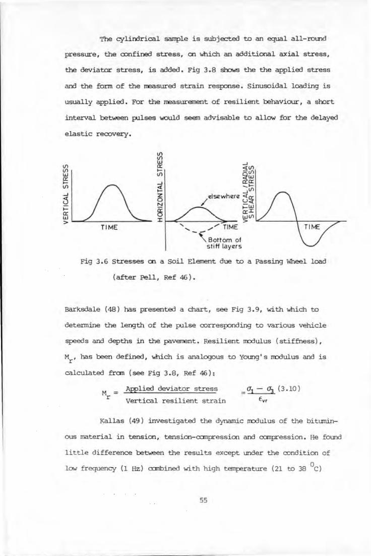
The cylioorical sample is subjected to an equal all-round

pressure, the confined stress, en Which an additional axial stress,

the deviator stress, is added. Fig 3.8 sh:)ws the the applied stress

and the form of the rreasured strain res.r:onse. Sinusoidal loading is

usually applied • For the rreasurement of resilient behaviour, a short

interval between p.Jlses would seem advisable to allow for the delayed

elastic recovery.

1/'1 1/'1 w _J

1/'1 a:: <((/) 1/'1 1-

~~ w 1/) a:: 1- _J 1/)

~ .._I-_JI/'I

_J z ~tlsewhere <(~ j 0 / ~ N 1-

~ ._w

a:: a:: I w I

Wll'l > >

TIME ' _,,TIME ...... --'Bottom of

stiff layers

Fig 3. 6 Stresses en a Soil Element due to a Passing Wheel load

(after Pell, Ref 46 ) •

Barksdale ( 48) has presented a chart, see Fig 3. 9, with Which to

determine the length of the pulse corresponding to various vehicle

speeds and depths in the pavement. Resilient rrcdulus (stiffness) ,

M , has been defined, Which is analogous to Yotmg' s rrcdulus and is r

calculated fran (see Fig 3 .8, Ref 46):

M = r

Applied deviator stress

Vertical resilient strain

= a1 - a3 ( 3 .10 )

Evr

Kallas (49) investigated the dynamic rrcdulus of the bitumin-

ous material in tension, tension-cx::rnpression and canpression. He found

little difference between the results except under the condition of

low frequency (1 Hz) a::::mbined with high temperature (21 to 38 °c)

55

when the dynamic tension or tension-a::rnpression m:::x:Julus a:>uld be as

low as one half of the dynamic a::rnpression m:::x:Julus. The De£lect.ograph

(18) rroves at al:x>ut 2 Krn/hr, i.e. loading of low frequency, and it is

0 usually operated at an average temperature of 25 c. Therefore,

under these loading a:>nditions the dynamic m:::x:Julus (stiffness) of the

bituminous ma.terial should be determined fran a::rnpression testing.

o-1 = Major princ1pal stress

cr3 = Minor princ1pal streg; =Cell pressure

(er,- cr3l = Deviator stress

Fig 3. 7 Stress System in the Triaxial Test

(after Pell, Ref 45 ) •

Bituminous a:>re samples obtained fran sane of the AASHO Road

Test pavement sections were tested under repeated load conditions to

determine dynamic a::rnplex rrodulus (stiffness) values (50). Each of the

a:>re samples were subjected to various loading conditions and tempera-

tures. The change in the vertical stress did not have an appreciable

influence in the dynamic m:::x:Julus; ro...ever, the dynamic m:::x:Julus signif-

icantly varied with a change in tem];Jerature (50).

56

The resilient rcodulus ( stiffness) , ~, obtained fran the

repeated load triaxial test is defined as the deviator (or repeated

axial) stress divided by the recoverable strain (or resilient strain),

associated with the l::ounce of the specimen (51). By definition, a

secant rcodulus is obtained that corresfOnds to the mini.mun value

ocaurring during the loading fX)rtion of the test.

q, : ~led devl<llo< stress

Gm= mo!Qn dev>olo< stress

jj~}} i i ~

VI ~~-----------------------

' s~----------------

€ ..... . €, ~ Reslltf'f"''t stro1ns

Ei> = ~ slron

Fig 3 . 8 Measurements in Repeated Load Triax ial Test with

Constant Cell Pressure (after Pell, Ref 46).

Kallas and Riley (52) carried out repeated load tests en

unconfined cylindrical samples of asphalt paving mixtures at several

temperatures. rhe resultant axial and radial strains were rreasured and

the dynamic a:mple x rcoduli and the Poisson' s ratio were detennined.

57

The vertical strains ....ere treasured with strain gauges cemented to the

specimen at mid-height with epoxy cerrent. The h::>rizontal strains were

rreasured with strain gauges cemented at mid-height to specimens, at

right angles to the direction of loading.

10~-------------------------------,

Vehicle speed .. ·~ : ~ 1.0

"' -~ .. > c .. ;; ~

" g

0.1

v • 72 km/h (45 mi le/ h)

Depth beneath pavement surface (cm)

Fig 3. 9 Variation of Equivalent Vertical Stress Pulse Time with

Vehicle Velcx::i ty and Depth (after Barksdale, Ref 48) •

Absolute values of the cx::mplex rrodulus (stiffness), ~r , and the phase lag, 8, ....ere calculated as follows (52) :

,Er=~ E~

(3 .11)

= absolute value of the ccrnplex rrodulus;

a~ = amplitude of the sinusoidal vertical stress;

E = amplitude of resultant sinusoidal steady state vertical ~

strain .

(3 .12)

where 8 = p-tase lag, degree,

t. = time lag between a cycle of sinusoidal stress l.

and the resultant cycle of sinusoidal strain, sec,

58

~ = time for a cycle of sinusoidal stress, sec.

The a::rnplex m::x:'lulus stiffness is found to decrease with

increasing temperature and with decreasing frequency, i.e. canplex

m::x:'lulus is dependent on temperature and loading frequency (52). The

a::rnplex m::x:'lulus increases with increasing vertical stress. Since the

increment is relatively small, the effect of the vertical stress on

the m::x:'lulus is not of practical i.fnt:ortance.

Khanna et al (53) detennined the stiffness of bituminous

material by triaxial tests. In a loaded pavement system, the vertical

stresses in the bituminous surface course are always campressive

whilst the horizontal stresses may be. oampressive or tensile in

nature. The condition when horizontal stresses are a::rnpressive, was

stimulated by triaxial tests. To stimulate horizontal tension in the

bituminous layer, a test method was developed making use of thick

hollow cyclindrical triaxial specimens. The specimens were subjected

to internal radial pressure and tested under axial a::rnpressive load-

ing. The stiffness was found to be dependent on the axial stress and

internal radial pressure. An analytical finite element m::x:'lel was

developed to predict load response characteristics of the multi-layer

pavement system. The stiffness detennined fran the above tests were

used as inputs into the analytical m::x:'lel to predict the load deformat-

ion resp::mses of the semi- full scale pavement test sections. The pred-

ictions fran the developed m::x:'lel show closer agreement with the exper-

imental result in comparison with classic linear elastic m::x:'lel (53).

Poisson's ratio is defined as equal to the lateral strain

divided by the axial strain.

Poisson's ratio may be calculated as:

J-t= Err · Evr

59

(3.13)

Poisson's ratio depends an temperature and therefore it has a minimum

value at low temperature and increases with increasing temperature

(46, 52). Poissan' s ratio also decreases with increasing frequency.

Tests carried out in a constant rate of strain tria.xial ccrnpression

showed that Poisson's ratio was essentially independent of rate of

strain, but at 4 QC had a value of approximately Q.35 and at 25 QC

and at 6Q QC a value approaching Q.5. When deformation is large, it

is fOSsible that "dilation" (volume increase) will occur and Poisson' s

ratio will exceed Q. 5.

3.3.3 Permanent Deformation.

3.3.3.1 Introduction.

A significant cause of pavement failure is the development of

excessive permanent. deformation, a rut, which at 10 mn depth is regar­

ded as critical and at 20 mn depth constitutes failure (54). The surf-

ace deformation is a summation of the vertical deformation developing

in each layer of the pavement structure. The viscous resfOnse of

bituminous materials can contribute substantially to the total defo~

ation recorded at the surface, particularly when operating under high

temperature conditions.

3.3.3.2 Creep Testing.

The simplest way to investigate the permanent deformation

characteristics of bituminous materials is by the use of the static

creep test. The Shell L:lboratories ( 40) conducted a large nurrber of

creep tests involving simple unia.xial loading in ccrnpression in order

to study the effect of mix parameters on permanent deformation. The

effects of temperature, binder type and applied stress can be ignored

60

if the results are plotted in tenus of a mix stiffness against binder

stiffness, see Fig 3.4. On the Sm against ~ plot, see Fig 3.10,

the creep results nove fran right to left since increasing time

i.nplies decreasing bitumen stiffness (55). Mixes ma.de with crushed

sand provide higher mix stiffness and therefore, lor....er pennanent

deforma.tion than mixes ma.de with rotmded sand • The canpaction trethod

and canpactive effort influences the density and the packing arrange-

ment v.hich in turn affects the mix stiffness ( 40) •

:.e . !; e Vi

~ g et

.€ 2 E

10

01

0~ '()'

'()Q

Vl 10

• • •

oo u

• • •

I • • • • · , T=:x:l"C

• 0 0 T = '()"C

0 0

oOO

0

• . o. . :)

• •

I i

Fig 3 .10 Creep Results (after Hills et al, Ref 55 ) .

Brown et al (51) carried out sane dynamic triaxial and static

creep tests en dense bitt.nnen ma.cadam and proch.x::edthe graphs in

Fig 3 .11. It can be seen that at low stress levels the static and

61

dynamic r e sults are similar . Ho....ever, at the higher stress levels , a

static s tress of only alx>ut 65% of the dynamic value .....ould be required

to produce the same strain at a . particular t.:iJTe . The effects of diffe-

rent stress levels and temr:erature (51) are shc:r,.,n in Figs 3 . 12 and

3.13.

--· r ; 1.0>1-----I 0

0 o.s ~ .. >

~· O·IJ - ·r·---

I ~ 0·6 - __ ..

1.

: I ! I 0 o., -- .. - -- +--c E? .. ~ 0 ·2

~ >

0 ___ .._ __ _._ __ __.

800 1000 ( kN I m 2 1

200 '00 600 100 WO Apploed ver1ocol slrt>Ss I kN / m 2 I

Fig 3 .11 Canparison of results fran Dynamic Tests and Creep

Test at 20 ° C (after Brown et al, Ref 51 ) .

62

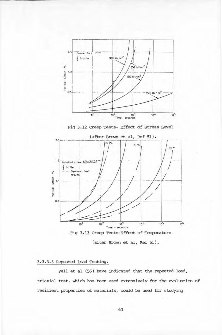
2·0

{ Scottt>r I

s 1-0 - ... -!:?

- [-----­~

0 1./ .. ..,.

0·5

i

I I ,_ ..

Fig 3 .12 creep Tests- Effect of Stress Level

I Scotl~r - - Oynomoc. t•st

r~sults

Fig 3 .13 creep Tests-Effect of Temperature

(after Brawn et al, Ref 51 ) •

3.3.3.3 Repeated LOad Testing.

Pell et al (56) have indicated that the repeated load,

triaxial test, which has been used extensively for the evalua.tion of

resilient properties of materials, could be used for studying

63

pennanent defonnation under I!Ore realistic conditions than those of

the creep test. Brown et al (51) have shOVJI'l that the pennanent strain

which gradually accumulates under repeated loading is essentially a

creep phenanenon. They studied the effects of vertical stress, temper­

ature, confining stress, frequency of the. vertical stress pulse, rest

periods and binder content by carrying out triaxial tests on dense

bitumen macadam.

BrOVJI'l et al (57) measured the sample defonnation over two

diametrically opposed gauge lengths about the mid-height of the

sample. The rreasurernents are thus free of specimen end effects and

errors which can be introduced by the use of an arbitary datum such as

the cell base or the cell lid. They used a set of three "strain

collars"; one pair measured the vertical defonnation while the third

I!Onitored lateral deformation (57). Four locating targets, glued to

the specimen, are at each end of the two gauge lengths. The relative

deformation of each pair of targets are rreasured by using a pair of

linear variable differential transformers (L.V.D.T). The central

collar is used for radial deformation measurement. It is a hinged

collar locating onto two diametrically opposed targets at the centre

of the sample. As the sample expands laterally, the gap between free

end of the collar changes and this change is rreasured by an L.V.O.T.

The samples were tested with lubricated loading platens to minimize

lateral end restraint.

Vertical stress has a major influence on pennanent strain as

indicated in Fig 3.14. The vertical stress applied consisted of a

30 KN/m2

constant value onto which the dynamic pulse was superi.mp:>­

sed (51). This value of "dead load" was in fact too high in relation

to the likely over-burden pressure to be expected in a pavement.

64

Cm~lonl Vl'rl slrl'$ 30 ~N 1m2

Unr.onlont! d 1 ~'r <"ou<"nc.y of YPrl ~lrt!S~ pulsl' 1 Hr

1.<, • l•mpProlur• ]() "C

f Sr.oltl'r

;f Fo olurt!

c 1-0 -- ----

~ " ~ ..

O·S ·-

Fig 3.14 Influence of the Magnitude of the Vertical Stress Pulse

on Vertical Strain (after Brov.n et al, Ref 51 ) .

Permanent strain increases with a decrease of application of

the vertical stress, i.e. the total loading time rather than the

number of load applications controls the permanent strain. Frequency

of loading between 1 and 10 Hz did not affect the relationship between

pennanent strain and time. Permanent deformation is time rather than

frequency dependent and the rest periods between stress pulses does

IX)t seem to affect the accumulation of strain.

The effect of static confining stress en the acc\..JT\ulation of

vertical strain under a repeated load testing is illustrated in

Fig 3 .15 • Similar effects were noted When the confining stress was

applied cyclically in phase with the vertical stress. Brov.n et al (51)

have rra.de a simplification to the test techniques to prodoce essentia-

lly the same response from the rra.terial by using a static confining

stress equal to the mean values of the desirable cyclic stress.

65

r-0)<'0mtC v~r l sin-ss 6SQ kl'll m2

1 .~ _Consta-t "'!r t sire$ 30 kN/m2 rrl'<)Jrncy 0 , VPr!lc;ol SlrP$ puiSP 1 Hl Temperature 20 •c

J ScoH~

r.ol---

10 I. 105 Cycl~s

Fig 3 .15 Influence of Confining Stress on Vertical

Strain (after Brov.n et al, Ref 51 ) •

Temr:;erature plays an imp:>rtant part in the build up of

pennanent strain, see Fig 3 .16. Resistance to pennanent deformation

cx:rnes fran a cc:rnbination of binder viscosity which is highest in the

rolled asphalt, and interparticle action, which is highest in the

dense bitumen macadam.

~

c e -;;

0 ~ ~ >

2.0.----- l 1---1·5

1.0

o.s

Oyt.-lrnr. 'Yf"'' t ~lr f""".~ Constant _, •tress UntonfonPd FrPQUl'l'<.y of ~rt . sir~ pulse t Hz

£ Scatter

* Fo~ure - r-·---

,

Fig 3.16 Influence of Temperature on Vertical

Strain (after Brov.n et al, Ref 51 ) •

66

Based on field studies, Chou (58) has suggested that the nost

critical conditions for bituminous material occurs in spring when the

subgrade normally contains excessive noisture and provides the least

amount of support and the bituminous material is relatively cold and

cannot withstand large strain repetitions.

3.3.4 Fatigue Cracking.

3.3.4.1 Introduction.

Under traffic loading the layers of a flexible pavement

structure are subjected to a continuous flexing with the life of the

pavement decreasing with increasing magnitude of stress and strains.

The magnitude of the strain is dependent on the overall stiffness and

nature of the pavement construction but measurement has indicated

tensile strains of the order 100 x 10-6

for a 3 ton ( 26.7 KN) wheel

load.

Service life (N ) is the accumulated number of load applie­s

ations necessary to cause failure in a test specirren. The fatigue

behaviour of a specimen subjected to repeated loading depends primari-

lyon the load, envirorunental and specimen variables. The service life

of specimens tested in the lal::oratory depends greatly on the node of

testing used, either controlled stress, when the loading is in the

nature of alternating stress of constant amplitude, or controlled

strain, when the loading is in the form of an applied alternating

strain or deflection of constant amplitude.

3.3.4.2 Effect of Stiffness and Criterion of Failure.

If specimens are tested in controlled stress, then for diffe-

rent stiffnesses, results such as those shown in Fig 3.17a are

67

obtained (46). At a particular stiffness, S, the mean fatigue lives

can be represented by a straight line on a log plot of stress, against

the number of cycles of load, N , to cause failure. Different levels s

of stiffness are represented by approximately parallel lines, showing

that with this type of testing the fatigue life is highly dependent on

stiffness, the stiffer the mix the longer the life. When the results

are replotted in terms of strains, as shc:J\..n in Fig 3.17b, it can be

seen that the results for different stiffness coincide, indicating

that strain is a major criterion of failure and that the effects of

tenr;erature and speed of loading can be accounted for by their effect

on the stiffness-strain criterion (46).

When similar specirrens are tested in a controlled strain rrcx:le

results such as those shCl'Wfl in Fig 3 .17 c are obtained ( 46 ) • Although

the lines coincide at higher stiffness, those at lower stiffness show

the reversed effect of stiffness from that found from co~trolled

stress tests. This is due to the different rrcx:le of failure developed

in the t'No tests. In controlled stress, the formation of a crack

results in an increase in actual stress at the tip of the crack due to

the stress concentration effect and this leads to rapid propagation

and ccrnplete fracture of the specimen. In controlled strain, the forma-

tion of a crack results in a decrease in stress and hence a slov.er

rate of propagation (46).

The criterion of fatigue crack initation is one of applied

tensile strain, and a general relationship defining the fatigue life

is as follows (46):

N = C x (1/E )m s

( 3 .14)

where Ns = number of appliC'!tion of loads to initiate a fatigue

crack (failure),

68

E = maximum value of applied tensile strain,

C, m= Constants Which depends on the mix. Characteristics.

For ITDSt dense mixes the factor, m, defines the slope of the strain-

life line. The slope of the fatigue line appears to depend on the

stiffness characteristic of the mix ancl nature of the binder; mixes

having high stiffness and linear viscoelastic behaviour giving a

flatter line. The behaviour is characteristic of mixes having a relat-

ively high binder content of a harder bitumen. Mixes with softer

grades of binder show considerable non-linearity, particulary at high-

er stress levels and they have a steeper fatigue line.

Kirk (59) reported that for a given mix, the initial strain

E ( N ) corresponding tD a given number of cycles tD failure is an s

tmequivocal function of the stiffness of the bitumen. E ( Ns) increa-

ses with increasing maximum size aggregate and decreases sharply When

the filler content is reduced below a certain limit. With a given

gradation containing sufficient filler, E ( Ns) increases with incre­

asing binder content. This increase is greater, When the. mix contains

a large mnnber of small voids. The at:ove effects are only valid for

mixes with a small number of voids (59).

3.3.4.3 Effect of Mix Variables.

It has been fotmd that the fatigue life of a mix at a certain

strain level may be increased by the use of a rrore viscous binder

and/ or an increase in the binder content. All other mix variables are

apparently secondary ahd only influence fatigue performance in so far

as they affect the relative binder content. It is possible to increase

the stiffness of a mix by changes in aggregate grading, but if the

relative binder volume is tmaffected, the fatigue performance at a

69

certain strain will not i.rrprove. It is also pJssible to increase thP.

Entigue life of a mix at a certain strain whilst reducing the stiff­

tra~itional ness by increasing the binder content beyond the~optimum. Therefore,

for good fatigue performance in association with rna.lCimum stiffness, a

dense grading is required in which the voids are filled with a hard

grade of binder ( 40 ) •

3.3.4.4 Prediction of Fatigue Performance.

Fatigue tests are carried out under simple loading conditions

that apply continuous cycles of loading of particular magnitudes under

controlled conditions of temperature and speed. In practice, the

material is subjected to a succession of load pulses of varying size

and with rest period between strain. Since stress controlled tests

essentially determine the time for crack initation, some allowance

should be made for the time it takes for a crack to propagate up

through the bi turninous layer . The results of simple loading tests iTli:ly

be used to predict the performance under <Xll'lJ:X)und loading condition by

the use of Miner's Law, namely (45): r

~l/N1 = 1 ;:1

where n1

= number of cycles of strain applied;

(3 .15)

N1 = number of cycles to pn:x:luce failure under constant strain

amplitude from simple loading tests;

r = number of different strain levels involved.

Chou (58) also suggested that when determining the pavement

requirements to prevent excessive strain in the snbgrade, the stiff-·

ness of the bituminous layer should be evaluated at the highest

temperature expected in the field, i.e. when the bi turninous material

contributes the L:~.~3t. .J:<nunt of resistance to deformation.

70

01 0

_J

( a ) log Cycles Ns

( b ) Log Cycles N s

( c ) Log Cycles Ns

Controlled Stress Fat igue Tests. At

Different S tiffnesses

S 1 • S2 Etc.

log o- v Log Ns

CcntroUed Stress

FatigtJe Tests

Log E v. Log Ns

Cont rolled Strain

Fatigue Tests

log E V log N s

Fig 3 .17 Effect of Stiffness en Fatigue Life Using Different

Mcdes of Loading (after Pell, Ref 46 ) •

71

3.4 Cement Bound Materials.

cement is utilised as a binder in material used for toth base

and sub-base layers, producing lean =ncrete, cement round granular

material and soil cement. Its ability. to resist cracking largely

depends on the relationship between its stiffness and strength. The

dynamic rrodulus depends on the type and content of cement, water

=ntent, aggregate type and grading (56)'. Its high value of stiffness

results in generatiTig tensile stresses of =nsid~rable magn itude due

to toth traffic and temperature. Fig 3.18 shows the relationship

between the flexural strength and elastic rrodulus. It also shows the

. a??roximate thermal and traffic stresses for same typical thickness of

lean concrete base. It seems that the a::rnbined stresses exceed the

flexural strength except at the high values. of rrodulus ( 60) • It is

=nsidered that a lean =ncrete base will probably be cracked (primary

cracking) to same extent due !!Ore to thermal effects than to shrink­

age before the pennanent =nstruction is compl~te. Further se=ndary

cracking may or may not occur depending on the magnitude of the

traffic-induced stresses. A reduction of approximately 30% in strength

can be expected under repeated loading conditions (61). It is suggest­

ed (56) that a rrodulus value of 500 MN/m2

and a Poisson' s ratio of

0.25 would be appropriate for design calculations.

Research (56) on soil cement under repeated loading and full

scale road experiments show that soil cement layers under heavy

traffic quickly becc:me extensively cracked. Therefore for design

calculations they should be treated as untound granular materials

having a rrodulus related to that of the unclerlying subgrade, and a

Poisson's ratio of 0.3.

72

_L 5000 OOmm

-, VARYING

-+ l..CX)() 250"'"'

N __L_

E SUBGRAOE 6 .,.

I BASE

ASPHALT

ITHICKN ::ss ----+-----------T---------~~~t25mm __ _

I ---~ CEM ENT OOUNO

BASE _, I ·- . ,..-. T25mm , I s~ ~e ----~----~~--~----~~ ,. I ,

C BR !50 mm

z ..X 3000

~ uJ

g: !___.C-.----- 200mn ~ 2000~----~~~~--~----~~----~~~-------------------­w -' ~ z uJ ~ JOOmm

-- STRESS DUE TO TRAFFIC - -- 5 TRESS DUE TO TRAFFIC

& TEMPERATURE

OL---------~--------~--------~--------~-----------0 10

DYNAMIC MJDULUS OF

20 30 40 ELASTICITY OF THE BASE ( GN 1m2)

Fig 3.18 Variation of Indoced Stresses and Flexural-Strength With

Elastic Modulus £or Various Lean Concrete Bases

(after Lister, Ref 60).

3.5 Cohesive SOil.

COhesive soil has an elastic rrodulus ....ni.ch is non-linear and

very much dependent oo stress. The non-linearity can be generally

represented by the curves in Fig 3 .19.

V)

Ill Ill 11 I 1/l

rr:: 0 1--<t > w 0

l~lrflE J\ '=, ING

\

(Otll lt~ING '•IHI :'",c; ( (J J )

~>I HAIN (€)

Fig 3.19 The Effect of Stress Condition oo the Resilient Modulus

of Cohesive SOil (after Pell et al, Ref 56 ) •

73

3.5.1 Resilient Behaviour.

The resilient rrodulus of silty clay is of the form (40):

( 3 .16)

where a;= inital effective oonfining stress,

'lr = cyclic deviator stress,

K, n = oonstants which depend on soil type and test oonditions.

The load frequency of be~en 1 and 10 Hz has little effect on resili-

ent strain. The resilient rrodulus will tend to be l<:l'v..er for load tests

with rest periods than for those obtnined fran continously loaded

tests . The rest period allows sane elastic recovery in the clay.

Confining stress does not influence the resilient rrodulus significant-

ly but the deviator stress does. Fig 3.20 illustrates the dependence

of resilient rrodulus on the deviator stress for a ,partially saturated

a::xnpacted sil ty clay ( 61 ) • Fran the tests carried out on ooth

100

... 80 E -z

:L

Ill 60 ::;)

\ J I V3 = 21. kN 1m2

\ '"5 "0

~ 1.0 c

.!1'

.in <11 a::: 20

~ \ r-. n ..0-

0 50 150 200 250 a:.- a3

Fig 3.20 Resilient Modulus of a Saturated Silty Clay as a Function

of Deviator Stress (after Seed et al, Ref 62) .

74

saturated and partly saturated soil, it was fotmd that it is the

inital effective stress that influences resilient characteristics.

This stress is the one to which the elements of soil are subjected

prior to the application of wheel loading. The magnitude of this

stress depends on the _p;:Jsition of the water table and the depth of the

elements. For deep water tables, high suction will develop and the

magnitude of the suction may be taken as equal to the effective

stress. Resilient m:xlulus is related to soil suction. For high water

tables, it is _p;:Jssible to estimate the negative _p;:Jre pressure and

hence effective stress of the water tr.lble present (40).

(3.17)

where 0]= applied confining stress;

U = initial _p;:Jre pressure;

aJ ::::: S, Suction, for deep water table •

The elastic m:xlulus may be estimated from the relationship between CBR

and dynamic m:xlulus (resilient m:xlulus) obtained from Wave Propagation

testings (63) which is usually defined as (44, 64, 65):

Mr = 10 X CBR (ffim-2 ) (3.18)

although alternative m:xlels based on _p;:Jwer ftmction have also been

prOp:JSed ( 66 ) :

11 = 17.6 X (CBR)0 "64 (MPa) r

(3 .19)

The elastic m:xlulus of clay can also be determined from the

Plasticity Index (I ) based on reseach at TRRL (67, 68): p

Esubgrade = 70 - Ip

where E is in MPa and I is a Percentage . p

(3 .20)

Kirwan et al (69) have developed a chart for the prediction

of resilient m:xlulus of glacial till soil from IIDisture and density

information _for the plasticity index range from 14 to 20, see

75

Fig 3.21.

.Poisson' s ratio of 0. 5 will be applicable to the saturated

condition under urx:kained ronditions. r...o...er values will apply as the

degree of saturation decreases and 0.4 is often taken for design purp-

oses.

1· 1

c .2 ~ t-o c.. E 0

" .. >

] 0·9

"" «

Relative moisture content , Rw

Fig 3.21 Relationship Between Relative Canpaction, Relative Moisture

COntent and Resilient Modulus (after K.irv.an et al, Ref 69 ) •

3. 5. 2 Pennanent Strain.

Pennanent strain under repeated loading depends on the appli-

ed deviator stress and also on the stress history, density and noist-

ure a::ntent of a soil. A definite failure FOint can be established

when the rate of permanent deformation shows a sharp increase which

can be seen fran the relationship betv.een permanent strain and nurrber

of stress applications for normally ronsolidatee sil ty clay, shown in

Fig 3. 22. The concept of ' threshold stress' has been used to define

the l::oundary between ' stable behaviour' , where no failure will occur,

and 'unstable behaviour' , where, provided sufficient applications of

load are applied, failure will eventually cx:cur (56). For heavily

over-c:onsolidatea clay, a well defined failure condition is rXJt

76

reached, but strain levels are about twice as high as in the normally

a:nsolidated case. Hyde et al ( 70) have sho...n that reasooable predic-

tion of permanent strain rate under repeated load conditions can be

obtained fran the creep tests. NUMBER OF STRESS REPETITIONS

10 10 2 103 ot. 105 0

~ ·5~------+-------1---~~+--------r------~~--~~~----~

<t -fE tJl

~ ·75~------+-------~------~-------r-------;-----~----~ w z <t ~ er

R = MAX . APPLIED DEVIA1CR STRESS .d:X)

Ul\ffiAINE 0 SHEAR 5 TREt-.GTH R = 92 "1. = 7 s .,. w 1·00 a.

1· 25L-. ______ ...!,..._ ______ ......_ ____ ......_ _____ __.._ ______ __. ______________ ____,

Fig 3. 22 Relationship Between Permanent Strain and NUmber of

Stres~ Applicaticn for a Normally Ccnsolidated

Saturated Sil ty Clay (after I.ashine, Ref 56 ) •

3.6 Granular Material.

Granular materials are successfuly used as load distributing

layers in the pavement structure. Well ccrnpacted granular .materials

are effective in reducing the stresses transmitted to the generally

weaker subgrade. Granular materials generally contain water in their

pore spaces and extensive repeated load testing has revealed that the

resilient rrodulus of elasticity is very stress dependent. The non-

linearity is represented by the curves in Fig 3. 23 •

77

3.6.1 Resilient Behaviour.

The resilient rrodulus of elasticity being a secant nodulus,

is a function of both deviator and confining stress. In general, the

nodulus depends on l:oth shear stress ( q/2) and mean nonnal stress, p,

which is related to confining stress.

(3.21)

where q = Deviator Stress, p = Mean Nonnal Stress,

a1 = AXial Stress, a2 = a3 = Radial Stress.

Nonnal stress level has the greatest effect in defining the m::x'lulus

than shear stress. The non-linear behaviour can be expressed in the

fonn:

where E = resilient modulus; r

(J = sum of principal' stress = 0). + 21J2= q + 3Cij;

(3. 22)

Kl I rs = constant which depends on the material and test

condition.

More recent research (71) has shown that the resilient behaviour is

rruch l!Dre cx::mplex than Eqn ( 3. 22), but under conditions well r~ved

fran failure, this equation seems to be valid. Frequency has little or h

no effect on the resilient strain, although only limited experimental

evidence of this is available. The stress history does have sane

effect on the resilient behaviour. Boyce et al (71) found that the

resilient stress decreases and reaches a steady value after about 200

to 1000 cycles, without any substantial increase in pennanent strain.

It was suggested (70) that resilient str~in 1neasurement should be

taken after a few cycles (about 4) on each stress path.

78

bu \CAEASII;r,

tJ) er)

j VI ltJ 1-l/)

I'" z ::J Ill ~_J

_j::J n: 8]8 0 ~- cr::f <{

> w 0

SlR.i\IN (€) <11

Fig 3.23 The Effect of stress Ccndition on the Resilient ~ulus

of Granular SOil (after Pell et al , Ref 56 ) •

In-situ investigation using the Wave Propagation technique

has indicated that the rrodulus of elasticity which a granular layer ;:1

develops is dictated by the subgrade suPfOrt conditions (63). In

practice, the rrodulus is rx:mnally estimated using Eqn (3.18). Field

measurements (63), together with theore tical analysis (72), SUCBest a

nroular ratio of two (42) W"lilst other investigations (73, 74) SUCBest

that the rrodulus of the granular layer, E2

, is influenced OOth by

its layer thickness, H2

, and the rrodulus of the tmderlying layer,

E2 = IS E3

where IS = 0.2 H2°·45

(3.23)

Limits on the application of this approach have been profOsed

for situations in which rrore than one layer of granular material is

laid (44). These limits, ba.sed on the application of elastic theory,

suggested that multiple layers act as a a:m}X)site material for which

the ratio of the subgrade rrodulus to a::rnbinedrrodulus of the granular

layer is tmlikely to be greater than about 4 (75). HCJ~.o.ever, results

have been ref()rted (76) W'lich show' that, on the ba.sis of measured CBR

79

values, higher ratios up to 5 ar 6 can be generated.

Poisson's ratio depends on the principal stress ratio ar

ratio of deviator stress to mean nonnal stress, P (= 1/3() ), with a

better defined relationship resulting from the use of effective stress

rather than total stress (40). Its magnitudes increase with increasing

~ (i.e. cyclic deviator stress)/P, but a value of 0.3 seems most

appropriate for design. Resilient rrodulus and Poisson' s ratio also

depend on the aggregate grading, density, particle shape, texture and

moisture conditions. Higher density produces higher resilient rrodulus

and the dependence on nonnal stress is greater with rounded aggregate

than with angular aggregate.

3.6.2 Permanent Strain.

The relationship between permanent deformation and the number

of loading cycles for granular material is shown in Fig 3. 24. There is

a sharp increase in permanent defamation during the early load cycles

followed by very little subsequent increase, so the material reaches

an equilibrium strain. The value of this equilibrium strain depends on

the ratio q/a3

under drained conditions.

3. 7 SUITmar¥ of Procedure to Detemine Material Properties

for Pavement Design.

The procedures available to detemine material properties for

the purposes of pavement design are sl.ll1111arised in the following sect­

ions. Those procedures used to estimate materials properties in devel­

oping the rrodels used in the work described in this thesis are denoted

by *, while those used in validating the rrodel are denoted by **

80

5.---------,---------,--------.,--------~

~

12~---~-----~~--+---~

I -~------~----__1 ______ ~

0

s~~-~~~~~~~~ 1'4<'0"1 COl~ • •"9 SI~..S

Fig 3.24 Permanent Strain in a Granular Material as a Function

of Applied Stresses (after 8rO'w'l1, Ref 40).

3 . 7 . 1 Bituminous Material.

Stiffness.

(a) Use :

( i) Van der Poel' s Narograph (bitumen stiffness, Ref 41) with

either (a) The equation derived by Heukelan and Klanp (43),

Eqn (3.7),

or (b) Mix Stiffness Narograph ( 44) ,

(ii) Equation derived by Br0wt1 (45), Eqn (3. 9 ),

(b) Measure Stiffness Using:

( i) Creep under ronstant strains;

( ii) Stress relaxation under constant strain;

(iii) Constant rate of strain;

81

*

**

*

(iv) Dynamic tests under sinuosidal stress or strain; **

(v) Dynamic tests under repeated step function pulse loading.

Poisson's Ratio.

(a) Generally assumed (45) as 0.35;

(b) Measured fran experiments.

Permanent Deformation.

(a) creep testing;

(b) Repeated load testing.

3.7.2 Cement Bound Materials.

Stiffness.

(a) Measured fran experiments.

Poisson's Ratio.

(b) Generally Assumed (56) as 0.25.

Permanent Deformation.

(a) Measured fran experiments.

3.7.3 Cohesive Soil.

Stiffness.

* ** I

(a) wave Propagation test (63, 64, 65), Eqn (3.18);

(b) M:del based on Pov.er function (54). Eqn ( 3.19);

(c) Based on Plasticity Index (67, 68), Eqn (3.20);

(d) Measured Stiffness.

Poisson's Ratio.

(a) Generally assumed (56) as 0.4 £Or design purpose;

(b) Measured •

82

* ** •

* ** •

Permanent Strain.

(a) Measured fran experiments.

3.7.4 Granular Soil.

Stiffness.

(a) 11easured fran experiments,

(b) Eqn (3.23), (73, 74).

Poisson's Ratio.

* ** ,

(a) Generally assumed (56) as 0.3;

(b) Measured fran experiments.

Permanent Strain.

(a) Measured fran experiments.

* ** ,

CliAPI'ER 4 • 0 SELECI'ION OF STRUCI'URAL MJDEL.

4 .1 Introduction •

In recent years, highway engineers have shown considerable

interest in developing a mechanistic basis for designing and evaluat­

ing pavement structures. Theories based on linear elastic, non-linear

elastic or viscoelastic layered systems, together with linear elastic

half spaces, determined using Equivalent Layer Thickness concept, for

the prediction of pavement resp::mse, are all currently either in use

or under developnent (48, 77, 78, 79, 80). The finite element method

of analysing the pavement structure is aiS.o used, because of. its

ability to aca:::tmoJate non-linear materials properties that are stress

dependent and because it is capable of analysing structures with more

canplex loading and boundary conditions. Many of the design systems

~ing developed now include guidelines regarding the selection of

appropriate materials properties and the design criteria for use with

that system. sane of the theories and canp..~ter programs available to

analyse the pavement structures are discussed briefly in the following

sections.

4. 2 Linear Elastic Half-Space Theory.

Boussinesq ( 77 ) developed a theory for predicting the stress

distribution in a perfectly elastic, harogeneous mass which extended

infinitely in the horizontal directions and obeyed Hooke's Law. The

load is applied orginally as roint load and subsequently extended to

a circular contact area with unifonn pressure. This theory is not

capable of analysing a multi-layer elastic structure directly unless

84

the multi-layer elastic structure is first transforrred into an equiv-

alent semi-infinite space and then analysed using Boussinesq's equat-

ions (77). This transformation is achieved by using the Equivalent

Thickness Theory (80).

4. 2 .1 Equivalent Thickness Theory.

The basic .asstnnpt.ion is t.hn.t the stresses, strains and defle-

ctions below a layer will be unchanged as long as the flexural stiff-

ness of the layer remains constant. The flexural stiffness is a funct-

ion of the cube of the thickness of the layer and its rrodulus of

elasticity and Poisson' s ratio. The equivr.~lent thickness, He' of the

(n-1) layers at.ove layer n, is defined as follows (80, 81, 82, 83, 84,

85): n-1

He= f lC ~Hi lC .:;Ei (1 - Jln)/En(l - J.L;) (4.1)

where f = correction factor.

It can be represented diagrammetri~lly ~s shown in Fig 4.~.

~-:3_~~!:3 __ --

E3 /).3

Fig 4.1 Diagrammatic Representation of The Equivalent Thickness

Theory.

Boussinesq' s equations (77) are used to calculate tJ1e ~tress and

strains at the tmderside of the interface. Where Poisson' s ratio is

not 1<nown, the transformation may be sirr1plified by assuming a single

value for all the layers. For a multi-layer system, it is assumed that

85

the material below the layer oonsidered, has the same rrodulus as the

layer oonsidered. Results obtained via the EquivalenL. Thickness

method deviate from the exact layered elastic theory (80), Bisrro

(85). For better agreement, a oorrection factor, 'f', is introduced.

The oorrection factor is 0.8 except for the first interface where it

is 1. 0 • For a two-layer system a factor of 0. 9 is often used •

The accuracy of the equivalent layer rrethod reduces as the

number of layers increases (83). The main advantage of the Boussin­

esq's equations (77) is their relative simplicity which provides easy

access by practising Engineers. It would be advantageous if a simplif­

ied design procedure oould be developed, to satisfy the relationships

derived from the 3D finite element rrode 1 ( see Chapt • 7 • 0) , using the

Equivalent Thickness theory.

4. 3 Elastic Theory.

. This rrethod is inoorporated in linear layer elastic theory

and the finite element method. The finite element method can be used

either to carry out linear or non-linear elastic analysis.

4 • 3 .1 Layered Elastic Theory.

Since Burmister (77) first used elastic theory to formulate

equations for the deflection and stress in aircraft runv.e.ys in 1943,

there have been enormous developnents in the analytical design method

for pavements. The assumptions that Burmister (77) and others have

made are as follows :

(a) Each layer acts as a oontinuous, isotropic, homogeneous, linearly

elastic rredilllTl, infinite in the horizontal extent;

(b) The surface loading can be represented by a uniformly distributed

86

vertical stress acting over a circular area;

(c) The interface a:>nditions bet"Ween layers can be represented as

being either perfectly srrcoth or perfectly rough;

(d) Each layer is continuously supported by the layer beneath,

(e) Inertia forces are negligible;

(f) Deformations throughout the system are small;

(g) Temperature effects are neglected.

several different rrrulti-layer elastic theories have been

proposed in recent years by different authors who assigned different

properties to the uppermost layers. Westergard (87), Hogg (88),

Odemark (88), Pickett et al (88) have treated it as an elastic plate.

Tables 4.1 and 4.2 (88) gives brief details of the type of analysis

carried out by each of the authors. Bunnister (89) and Hank et al (90)

have treated it as an elastic layer. The differences bet"Ween the two

approaches is that an elastic plate is subjected to bending deformat­

ion but suffers no vertical deformation due to direct stresses,

whereas in an elastic layer all the stresses are considered and no

restrictions are placed on the deflections.

Measurements of the vertical deflection of a flexible pave­

ment under moving wheel loads carried out by the TRRL and WASHO shows

that transient compression of the upper layer occurs, indicating that

it behaves as an elastic layer rather than as a plate. Burmister's

theory (88) treated the road as a system with three elastic layers

with rough interface. Jeuffory et al (88) assumed the top layer to be

an elastic plate and the middle layer t0 be an elastic layer with no

friction at the upper interface and perfect roughness at the lower

interface. The interfaces occuuing in practice are unlikely to be

ideally rough, but t..'1ey are also far fran SIIDOth.

87

A)l,."'med cond1110n1 AJ;&umed condtUon Form ot loadtnc f'aramct~r• uae-d

Sut-u~• and d~lft'-Commmt& AuthOr of lh~ Inert at \h~ lntf'rfarc I ton. d~lf'rtatltftl

Wut•ruard(2) £tulle pial• on 1 011t'OnUnVO\II Untform, carC'\&Ju M•odul u1 of e®cr ad• T~nstl• .,,,,......,,at 1W ~:w:IC' IS W\t~a . .h&II C

(1828) •uot::nd• arttnt: u loadu\c. ructton . (1. e . thr.-" pot.nta on tiW ..,.. ctressea tn th• t~o~o.cradr

a ,.~ne& of p.ar.aHel •vr•nc ron•t~t) •urhc• ol t..hr pbtt'. ~--~•d•rf'd. verttca.J , tnd~~ndf'nl IPflt\CS.

Ho,..lll EIL'\IIC platf' on 1 - - Younc'a modulu• and T•:u ll# 1-lr~•....,. lA l:.a~&KJf'l O'f w"''~rrurd' • (I ill) ••:~'ll ... tn.Jtnht Po•~r~~.on · a raun lor lhr pJ.ar•. .......,_

elutlc tuiJJTadr . thf' •ubtT.adc .

BurmtsterC4) [ lullt' I.Jyn n n a a) Conunuoua Brurl (unct•on a . £ 1 w . u .,rr . n. u. tW t:qu..ltwta dertvf'd but not (19~ll &f'mt-tn.hmlf' ela~uc. bt Ot•C'onHnuov~o luadlnJ • r2 ~\·r mcnt ...,.S tM : •• ,.a,h:atf'd lor apeoc1ftC

lu~rade. . aubt:'fad•.

.,. __ ro.C~l .. - Unllorm, Circular - rAJ I SIJ'P'\•'• ln lM "Ea~to:t .and numf'na..l (1~1) lua.chft(". l p.~,C"mrnt .and "aluan~ of 8t.::-a:u1Hu'a

aut,p-ade. -'-

• Hantt (. - - .. - Str•s!l•• at b:xll -f;c:rtvn•.,.(6) atdu of Uw

(1941) lnt~rJillet.

l'lc •011 " Al(71 Eh.~uc platf' on a a) OiscontunKNS - /b ~d funC1tona AJJ stres••• and v.naJr Ap~tcabl f' t,o (1~8) serat-t.nhnue f'lasuc b) No horu.onta.J ol E:l/£2•1-'1 ddi~C'11on LD ~~ po•rmrr.U. ~oultl

Sl.lbfl'ade. · dts.plac•ment at and 1'2·

the au~acM. .,..,.... mnd~.!l f'd 10 6liO'W' lor t.hr tnterface. ~ la lhe Jla''«":nmt on

c6d'lft1,mt, and horuonuJ j-twar a1 t.M tntf'rbce , b)• ma~ thrm .at;T~f' ,,Lb 'B.o.nb•atc1' ' • re•:..du (appro•

Od•muk(l) - Ot&rontlnUO~o~a

I - - - 'Den u ."uona at u.

(IH!II aurfa<"• .and rad.W atr~s• at lhfo ~ of 1.h4' uppn layoiT.

Table 4 .1 Elastic Theories of 'lWO Layered Systan

(after Whiff in et al, Ref 88) .

.AssumC"d condttlons Assume-d cond.auon For m ol lo:adtnc P4.rasneu~rs u1~

StU5U'$ v.d drflt-c ... Comme'\t& Author of the layers illt the \nterl:~~ ttons dctermll\ed

Burmtster(9) T ... "' •la.suc l ayers on ;a_) Continuous tBeurl function ! · ~1· £1, £2 Ocflrcuon at the fA m., hod of al-(li~SI .a stmt-u\drflntlf' b) Otsconunuoua oad•nc • h2 h2 f2 El arc-ond interbcr. ""'lattl\1; all lbr

lslrtSSH 11 l'"f'f\ !but no nurnrrtcal ~va.Ju:auon of t.M ~•flrctton o r ~lrt"$Sf'S •

Hank C: .. Conttnuous . ~nlfonn ctrcub.r - All lbr strusrs at E.x\rnston and Scrn·n~r(6) o:adinc. lh• hrtt surface. ~um~rr1CU ~rva.J.u ... ,

(19~8) ~uvn o( Burmaatrrs t:-quat h>ns for lbc

(ID)'

l ret lntcrlace.

AL"Um £: Ft ·&. - a) ContlnUCN& - - VcruuJ Vtd radlal E..lrtcn1ton :a.nd (1951) alrt'&sce al. botb numcrtcU •vaJu-

antcrface1. ~tlon• et Burm•stcr's rqt.t.a-tons for verttc3.1

and radt&J. atrrl&ca:.

J<ulfroy C:(ll) E lastic plarr on an OlsC'Onhnuo~o~s at - ~· _!!j( E1 )1, ~-El "1· rq and u .2 &ch#lrt . rlut1c hycr on a U\r hrst tntrriace.. • • (ll.21 Ez·El

(19~7) ecmt-lnJtntt• clasttc conttnUOUI at ltlc IU~T).dC. accond lnter(acc.

Table 4. 2 Elastic Theories of Thr~ Layered Systems

(after Whiff in et al, Ref 88 ) •

It is justifiable to treat the flexible pavement as a three

layer system, wi. th the whole surfacing ( v.earing course and base

course) as the uppenrost layer, the road base as an intennediate layer

88

and the soil subgrade as fanning the lower semi-infinite layer. In the

paper presented by Acum et al (91), the authors published the inter­

facial stresses in a three layer system on the vertical axis through

the centre of the tyre contact area. The analysis was based on the

equations developed by Bunnister ( 77 ) • The loaded area was assumed to

be circular and subjected to a unifonnly distributed pressure. The

equation, first solved by Bunnister (77), defined the deflection, D,

of a t'w'O layer elastic system of pavanent in terms of its thickness,

H, and. its nodulus, E1

, laid on subgrade of nodulus, E2, and load-

ed over a circular area of radius, a, with an applied pressure, P •

This equation is of the fonn (77):

D = P.f [ (a/H), (E/E2 ), (l/E2 l J (4. 2)

It is possible to solve this equation to find the values of E1 and

E2

by measuring values of deflection obtained from two sizes of

loaded area. Similarly a three layer system is theoretically treatable

by using three loaded areas.

The advances in computer technology has overcame the difficu­

lties in solving complex mathematical equations. Shell and Chevron oil

companies have considered the pavement as a multi-layered elastic

system and have developed computer prograrrrnes known as BISAR (Shell,

Ref 30 , 44 ) and the ClfEVIDN (Chevron, Ref 92, 64 ) .

4.3.1.1 Elastic Theory Approach.

Tables and charts of influence values for detenninirgstresses

and deflection in a variety of two layer systems have been given by

Bunnister ( 77, 89 ) , Hank et al ( 90) and Fox ( 93) • For three layer

systems tables and graphs have been presented by Acum et al ( 91 ) ,

Jones (94) and Peattie (95). All these authors assumed a unifonnly

89

distributed, vertical surface load acting over a circular area and a

Poisson' s ratio of 0. 5 for each layer. Influence values were given

only for r;oints along the axis of symnetry.

coffman et al (88) a:mpared the deflection measured at the

AASHO Road Test with deflections calculated from results of laboratory

tests in order to verify layered theory. A three layered elastic

system was solved with tables prepared by Jones ( 94) and Peattie ( 95 ) •

Bases, sub-base and subgrade materials were characterized by creep

tests and the results were transformed to a dynamic rrodulus. The

dynamic rrodulus of the asphalt concrete surface was determined by a

cyclic triaxial test.

Brawn et al (96) also verified elastic layered theory in a

carefully controlled laboratory experiment, u·sing a program developed

by Jones (96). They found that elastic theory predicted vertical and

maximum shear stresses and maximum surface deflection satisfactorily,!·

Klomp et al (97) used the Shell Brsroo (86) program to a:mpare pred­

icted applied strain in the asphalt round surface and base layers with

values measured by wire resistance strain gauges. Flexural tests were

used to detennine the rrodulus of the asphalt round layers and 1</ave

Propagation technique was used for the subgrade. They found that

strain in the round layers could be predicted with reasonable accur­

acy. However, surface strain measurements traditionally have been rrore

difficult to predict because of the effects of the factors including

tyre profile, temperature variations and tensile stresses in the

asphalt concrete •

Throv.er et al (98) have also presented evidence indicating

that layered elastic theory can be used to predict stresses and strain

in pavements subjected to 'roving wheel loads. Dynamic m::duli of the

90

asphalt concrete were measured by means of a dynamic flexural test.

Sub-base m:xJuli were determined by wave Propagation technique and the

subgrade nmuli by the Shell correlation procedure and the measured

CBR value (98). There was gcxXl agreement between theory and measured

response for stiff pavement sections. There were sane discrepancies at

higher road temperature, partly because of the difficulties in evalua­

ting 'E' values of the asphalt concrete at high temperature.

Hicks (72), using classical elastic theory, predicted surface

deflection and strains in the asphalt concrete, strain in the untreat­

ed base layer and stresses in the subgrade with reasonable accuracy.

H<Jo,.ever, for the prototype pavement investigated, better a::rnparison

was obtained with finite element technique.

4.3.2 Finite Element Method.

The continuum mechanics approach described in the previous

section satisfies exactly the governing differential equations assoc­

iated with the pavement design problem but this is true only for the

case of haoogeneous, isotropic and elastic layers. The finite element

method on the other hand, offers the ability of nmelling pavements in

a considerably rrore realistic manner. Each element in the system can

be given independent anisotropic material properties and the layers

need not be infinite in width. SOlutions of the finite element fonnul­

ation for displacements, stresses and strains are obtained for each

element grid. In the elastic layered system, those quantites must be

calculated individually at each desired point. The finite element

method therefore provides an extremely JXlVoerful technique for problem

solving involving the behaviour of the structure subjected to acceler­

ations, loads, displacement or changes in temperature, but the method

91

is a numerical approximation, and as a result, the cost of ccrnputer

time to solve problems may be as much as ?. to 5 times that as for

classical elastic layered solution procedures.

Detailed description of the finite element metho:'l has been

presented by Zienkiewicz ( 99) , Nath ( 100) , Huebner ( 101 ) and Nay lor

( 102) • For the analysis by this method, the layered flexible pavement

is divided into a number of discrete triangular or rectangular finite

elements. Each adjacent element is inter-connected by frictionless

pins, called nodes. The structural stiffness properties of each

element can be determined by the application of energy principles

using an approximate displacement continuity inside each element.

Inter-element displacement canpatibility is il.lso nrunt.ained so that

gaps will not open up between adjacent elements. When a fine el<;!!llenl:

;:e.'>h size is used, the finite element theory will usually give a

satisfactory solution. Convergence to the correct solution with decre­

asing mesh size i.s ,,ot, ho~ver, al..ays guaranteed.

4.3.2.1 Finite Element Approaches.

Shifley (48) and !)mean (79) used finite element technique to

analyse pavement structures ccrnrnsed of an asphalt concrete surface,

granular l"O'l.dbase and clay subgrade. Shifley ( 48) conducted a series

of rigid plate repeated load tests on a full scale test section to

simulate slowly rroving traffic. Transient deformation cc:mputed fran

the results of the repeated load laboratory tests for multi-layer

pavement structures ccrnpared reasonably well with the measured test

road deflections. The non-linear behaviour for both aggregate base and

subgrade were approximately accounted for by an iterative finite

element procedure.

92

Duncan et al (79) analysed a pavement structure for OOt.h

st.mrner conditions (low asphalt stiffness) and winter conditions (high

asphalt stiffness). '!'he response of in-service pavements was calcula­

ted by an iterative finite element program together with material

properties detennined fran repeated load triaxial tests. Predicted

deflections were fotmd to be in good agreement with those measured by

the California Travelling Deflectaneter.

\'k)lff (103) canpa.red the stresses generated in three layer

pavements using a constant m::x:lulus of elasticity in the unbotmd

layers, with those generated when variations of m::x:lulus within the

layers were included. '!'he finite element method, using a load incre­

mental procedure, in which the total load is divided in equal incre­

ments and applied step by step, was used to analyse th-a pavement with

non-linear elastic behaviour. Wolf (103) · fotmd that the consideration

of the non-linear stress-strain behaviour of the unbotmd sub-base

results in completely different stress distribution in the whole pave­

ment canpa.red with constant m::x:lulus of elasticity.

Brown et al (104) used a pavement test facility for the

validation of the analytical design method. '!'he stress, strain and

permanent deformations of asphalt pavement with granular bases were

canpared with those camp.1ted by the finite element a:::mpJter program

called SENOL. Each structure has about 40 nm of asphalt, about 140 nm

of crushed limestone base and a silty clay !>Ubgrade of about 6% CBR.

Resilient strains were determined with a reasonable accuracy using

SENOL (104, 105 ) • Transient stresses were less satisfactory but perma­

nent strains and deformation were reasonably good.

93

4.4 Viscoelastic Layered Systems.

The elastic layered theory developed by Bunnister ( 77 ) ,

assumes that the material which constitutes the individual layers are

linearly elastic as characterized by the time independent constants of

prop:>rtionality tetween stresses and strains. This assumption is only

valid under dynamic loads with a relatively short loading time. Under

static loads of long duration, the stress-strain tehaviour relation­

ship of these materials will not te constant but vary with tirre. In

order to take this tirre dependency into a=unt, it was necessary to

renew the existing elastic theory and to develop the viscoelastic

theory. It has teen claimed by Monismith et al (78) that viscoelastic

theory would give a tetter approximation than the elastic theory for

predicting the jisplacement in a pavement system.

The viscoelastic analysis is quite similar to the elastic

~nalysis and based on the same assumption that prop:>rtionality exists

teo...een stresses and strains. However, the coefficients of prop:>rtion­

ality of the former are differential time operators whereas those of

the latter, generally referred to as shear and bulk rroduli, are time

independent constants. This principal of elastic-viscoelastic corresp­

ondence, as orginall y developed by Lee ( 106 ), has been used recently

by Huang (106), Ishihara et al (107), Barksdale et al (108) for the

analysis of the layered system. By applying the Laplace transfonnation

to the governing equations to remove the time variable, ~ viscoelastic

problem can usually te transformed into an associated elastic problem,

with a transformed variable. The solution of the associated elastic

problem, when transformed back into the real time variable, will give

the desired viscoelastic solution.

94

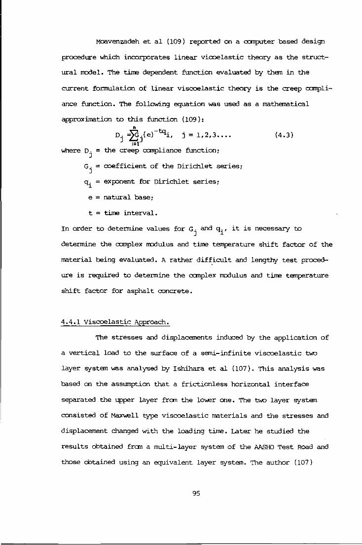
Moavenzadeh et al (109) reported on a CXIllpllter based design

procedure which incorporates linear vicoelastic theory as the struct-

ural node!. The time dependent function evaluated by them in the

current formulation of linear viscoelastic theory is the creep ccmpli-

ance function. The following equation was used as a mathematical

approximation to this function (109):

- n -tq. D. ~.(e) 1, j = 1,2,3 ••••

J i=l]

where D . = the creep cc:rnpliance function; J

Gj = coefficient of the Dirichlet series;

q. = extnnent for Dirichlet series; 1

e = natural base;

t = time interval.

(4.3)

In order to determine values for G. and q., it is necessary to J 1

determine the cc:rnplex nodulus and time temperature shift factor of the

material being evaluated. A rather difficult and lengthy test proced-

ure is required to determine the ccmplex nodulus and time temperature

shift factor for asphalt concrete.

4.4.1 Viscoelastic Approach.

The stresses and displacements induced by the application of

a vertical load to the surface of a semi-infinite viscoelastic two

layer system was analysed by Ishihara et al (107). This analysis was

based on the assumption that a frictionless horizontal interface

separated the upper layer fran the lo...er one. The t1.1.0 layer system

consisted of Maxwell type viscoelastic materials and the stresses and

displacement changed with the loading time. Later he studied the

results obtained fran a multi-layer system of the AASHO Test Road and

those obtained using an equivalent layer system. The author (107)

95

reported that the agreement between the theory and the test data was

quite satisfactory.

Barksdale et al (lOB) canpared measured and ccmJ;Uted resp::>nse

by using a linear viscoelastic approach. They calculated ooth pennan­

ent and resilient deflections for three layer systems on the AASHO

Test Road. The stress-strain relations were obtained fran the result

of repeated load triaxial tests. The calculated deflections were in

general close enough to suggest that viscoelastic theory can give

reasonable estimates of resilient and pennanent deformations.

Huang (106) developed two methods of analysis, one based on a

direct method of Laplace inversion and the other on an approximate

method of collocation. The two methods were used to detennine the

stresses and displacement in a two layer incompressible system, made

up of ooth simple and ccmplex viscoelastic materials. Both methods

agreed closely with a rnaxiroun discrepancy of not over 5%. The direct

method generally gives more accurate results and is applicable to the

case where the stress and displacement. equations can be reduced to a

fonn suitable for direct Laplace inversions. When a greater nunber of

layers and more complex materials are involved, such equations are

almost irrtpJssible to OOt.ain. Therefore the approximate method can be

used and it will give fairly good results.

4. 5 Theory Selection •

Pichumani (110) carried out a comparative study of several

compiter programs. The M'PAV ccmJ;Uter program, which is based on the

finite element analysis techniques, was shown to be more efficient and

econanical than the B!STR) (86) program for analysing layered pavement

system, loaded by a multiple wheels of modern aircraft. The stresses

96

and strains predicted by all the a::rrputer programs were similar, but

BISTRO (86) predicted slightly rrore deflection than the finite element

programs.

Duncan et al (79) carried out an analysis of a three layered

system using elastic half-space theory and finite element method.

for analysis of systems with linear material properties, the finite

element method offers little or no advantage over layered system

analysis. However, because it is feasible to incorporate non-linear

material behaviour in finite element analysis, the technique may be

used for obtaining solutions to problems which cannot be solved accur­

ately by other available methods.

It is the author's opinion that finite element method should

be used in the analysis of flexible pavement. This has the ability to

carry out non-linear analysis which enables it to incorporate non­

linear material properties. The canputing time required to carry out

such analysis is tremendous. Therefore, it would be very beneficial to

have sane sort of simplified design method based on results of the

expensive finite element method. To develop a simplified design proce­

dure, it requires the results fran a rrore soPhisticated and accurate

model against which the consequence of the simplification can be

judged and an estimate of error can be made.

One must not forget that at present electronic technology is

improving rapidly and in future even rrore pJwerful canputers are

likely to be developed. The canp.1ting time and the running cost will

be reduced considerably and every highway agency could be in a pJsiti­

on to afford a canp.1ter of low cost capable of carrying out finite

element calculations. Therefore, the exploitation of the finite

element method should not be abandoned.

97

The finite element rrethod has been adopted as the primary

analysis technique in the investigation reported in this thesis.

Although the analysis presented is limited to a linear system, the

model developed and results obtained provide a basis Dor further work

involving canplex and non-linear materials.

98

OiAPI'ER 5.0 FINITE ELEMENT ANALYSIS OF FLEXIBLE PAVEMENT.

5 .1 Introduction.

This chapter describes the use of finite element modelling to

compute tl1e stresses and deformations witl1in a pavement structure

subjected to. traffic loading. A suitable model is developed and calib­

rated by reference to the measured deflection profiles obtained under

field loading conditions. Finally, a procedure to convert absolute

surface deflection profiles predicted from the model into equivalent

Deflectograph deflections is presented including a description of the

appropriate computer programs,

5 • 2 The Finite Element Method •

The finite element rrethod is a numerical analysis technique

for obtaining approximate solutions to a wide variety of engineering

problems. The rrethod represents the extension of matrix methods for

skeletal structures . to the analysis of continuum structures. The

analysis of a continuum structure differs from those of the skeletal

structure in two basic aspects only, the subdivision into a number of

elements which are connected at the nodal £X>ints and the division of

the element stiffness characteristics. The finite element method is

essentially dependent for its success on the skillful use of comput­

ers. The method consists of reducing a structure to a skeletal form

consisting of individual members (elements) connected at their ends

(nodes). Analysis of the skeletal structure is carried out by first

considering the behaviour of each individual element independently and

then by assembling the elements together is such a way that the

99

following three OJnditions are satisfied at ~eh ~t<:'l<'liil p::>int:

(a) Equilibrit.nn of forces;

(b) Compatibility of displacements;

(c) Laws of material behaviour.

The finite element method is used in preference to other

nLDnerical methods for the following reasons:

(a) OWing to flexibility of their sizes ~nd shapes, finite element is

able to represent a given body more faithfully, ~ver ·complex

its shape may be;

(b) Time dependent and non-linear material properties can be dealt with

relatively easily;

(c) Botmdary OJnditions are dealt with easily;

(d) The versatility and flexibility of the finite element method can

be used very effectively to evaluate accurately the cause and

effect relationships in a complex continut.nn .

5.2.1 Basic Structural Analysis.

The Principal of Virtual Work (111, ll2, 113) is used in

deriving the stiffness properties of various elements. The principle

is OJncerned with the relationship which exists between a set of

external loads and the OJrresp::>nd ing internal forces, and also with

sets of joint (node) displacements and the OJrresp::>nding deformation

of members which satisfy the OJnditions of compatibility. The princi­

ple may be state<l as follows; 'The virtual work done by the external

loads is equal to the interna 1 virtual work absorbed by the struct­

ure'. The forces and displacement may be either ren.l or virtual but

the OJnditions of equilibrium and compatibility must be satisfi~i.

lOO

It can be expressed as:

E.D = JVI.e.V

where E = systems of external load>;;

D = deflection of the loads;

I = systems of internal fOrces;

e = internal deformation of ~.he >;tructure;

V = volt.nne of the structure.

The matrix rrethod may be fOrmulated in thrHP. different ways:

(a) Stiffness (displacement) method;

(b) Flexibility (fOrce) method;

(c) Mixed rrethod.

(5 .1)

In the >;tiffness rrethod, the displacements CDnp3.tibility

oonditions (deformed stn1cture must fit together) are satisfied and

the equations of equil,ibrium set up and solved to yield the unknov.n

nodal displacements. In the flexibility method the conditions of joint

equilibrium (internal fOrces balance the external applied loads) are

first satisfied and the equations, arising from the need of campatib­

lity of nodal displacement, solved to yield the unknov.n forces in the

rnerbers. In ark1 i.tio11 to these tv.o basic approaches, in recent years a

mixed fOrmulation involving ooth approaches has also been used. Furth­

er information about these method>; i~ ~vailable elsewhere, see Ref

(112, 114 and 115).

5.2.2 Subdivision of Structure.

In a continuum structure, the continuum has to be arti.ficia-

lly divided into a number of elements called finite elements or discr­

ete elements, before the matrix methcx'l of o.n.-~lysi~ can be applied. In

reality, the elements are connected together along their ccmron

101

toundaries, but in order to make the matrix method of analysis possi­

ble, it is assumed that the elements are interconnected only at their

nodes. This rreans that continuity requirementsare satisfied only at

the nodal p::lints and this v.Duld make the structure very much rrore

flexible. In the finite element, the individual elements are constrai­

ned to deform in specific patterns. The choice of a suitable pattern

of deflection for the elements can lead to the satisfaction of same,

if not all, of the continuity requirements along the sides of adjacent

elements ( lll ) •

5. 3 The Finite Element Program (PAFEC 75).

The finite element program, PAFEC, is readily available on

the Plyrrouth Polytechnic main frame ccrnputer. PAFEC 75 (ll6, ll7, 118)

is a version of PAFEC Which has been designed so that users may input

data in a very straightforward manner. This is a very general program,

i.e. not specially designed for pavement design like the elastic layer

program, BISAR (44). All the information atout the rrodels is fed into

the program data file and the program creates atout ten output files.

Each of the output files or phases consists of various information

atout the rrodel and engineering analysis. The impJrtant phases for

analysis of the structure are phases 1, 2, 4, 6, 7 and 9. Detailed

description of each phase is given in Table 5 .1. The program has the

facility to restart a particular job and this enables various rrodels

of different material properties, pressure and restraint to be analys­

ed without the need to re-start the job fran the beginning. This faci­

lity reduces significantly the computing time required to analyse

rrost of the rrodels. The program has to be started fran the beginning

When the co-ordinates of any of the nodes is changed or When the

102

thic1a1ess of layers is changed •

PHASE Short Detailed description description

1 Read Data modules are read in,. default values are inserted and the modules are placed onto backing store. The NODES module is expanded so that all mid-side nodes are included.

2 PAFBLOCKS Any PAFBLOCK data is replaced by the full nodal coordinate and topological description of the complete mesh of elements.

3 IN.DRAW The structure itself is drawn. At this stage it structure is not possible to show any results such as

displacements, stresses or temperatures since these have not yet been evaluated.

4 Pre-solution In this PHASE the constraints on the problem are housekeeping considered and a numbering system for the degrees

of freedom is deriv~d.

5 IN. DRAW This PHASE is very similar to the PHASE 3 except constraints the constraints which have been applied are

shown. Conversley the degrees of freedom can be indicated on a drawing.

6 Elements The stiffness (or other such as conductivity, mass et c) matrices of all the elements are found and put onto backing store.

7 Solution The system equations are solved for displacements, temperatures or whatever happens to be the primary unknowns in the problem being tackled.

8 OUT. DRAW The primary unknowns in the problem (i.e. displacements displacements or temperatures) are drawn.

') STRESS The stresses are found

10 OUT.DRAW Stress contour, stress vector plots etc. are produced.

Table 5 .1 Brief Description of the Ten Phases of PAFEC 75 ( Ref ll7 ) •

5 • 3 .1 Method of Analysis.

The rrodel of the pavement can be analysed as a plane elastic-

ity problem or as a non-linear analysis. Plane elasticity problems

inv.olve continua ··. loaded in their plane and may be separated into t.....a

separate classes, namely.plane stress problems and plane strain

103

problems. In a plane stress problem, the a::mtinuum (such as a plate)

is thin relative to other dimensions, and stress normal to the plane

is neglected. In a plane strain pr:oblem, the strain nonnal to the

plane of loading is assumed to be zero. Neither the assumption of zero

stress nor zero strain in the direction nonnal to the plane of loading

is strictly applicable to the flexible pavement problem but all the

pavement models were analysed as a plane strain problem since it was

o::msidered to be a more realistic approach.

5.3.2 Basic Element Shapes.

Since the fundamental premise of the finite element method is

that a continULun of arbitary shape can be accurately modelled by an

assemblage of simple shapes, most finite .elements are geometrically

simple. For analysis with the PAFEC cx::rnputer program, the structure to

be analysed is divided into a series of quadrilaterals and/or triangl­

es. The basic element shapes which can be used for analysis of two

dimensional or three dimensional flexible pavement model are illustra­

ted in Figs 5.1 and 5.2. Triangular elements an enable irregular toun­

dary structure to be modelled and they are often used to model a circ­

ular structure. A set of functions, depending to the type of elements

used, is chosen to define uniquely the state of displacement within

each element in tenns of its nodal displaceillent.

The displacement function defines uniquely the state of

strain within an element in tenns of its nodal d isplac<>Jnent. These

strains will define the state of stress throughout the element and

hence also on its toundaries. The chosen displacement functions sati­

sfy the requir:ement of displacement continuity between adjacent elem­

ents and this will ensure that no gaps will develop between the edges

104

of adjacent deformed elements. The rectangular plane elasticity el~

ents are slightly nore accurate than triangular elements because they

assume a linear distribution of strain over the element, whereas tria­

ngular elements assume the strain is a:>nstant within the element.

3

311200

2

3

a

s 2

Fig 5.1 Two Dimensional (2D) Elements.

4

s 2

Fig 5.2 Three Dimensional (3D ) Elements .

105

5. 3. 3 'I\-10 and Three D.i.Irension Isopararnetric Elements.

Elements which have one midside node are known as 'parabolic

elAJn=!nts' and they offer better accuracy. Higher order elements with

more than one midside node are available but although they give better

accuracy per element it is doubtful if they offer any advantage on a

'fer node' basis. The shape of a solid element can be expressed in

tenus of an interpolation function, also known as shape function. The

interpolation function for the various elements are <IS follow (119):

(a) Linear = No midside node element;

(b) Quai'dratic = One midside nocled element;

( c) Cubic = 'l'\oJO mid side noded element.

When the shafe function defining the geanetry and the function <~r-e of

the same order, .~.he element is ea lled isopararretric. The isoparametric

element enables curve sided elements to be modelled. Isopararnetric

elements are used to model the flexible pavement. The sides of the

element are considerP.d to be straight when the mid-nodes of the elem­

ents are not specified in the pr-ogrrun.

i\ two dimensional (20) element has two degrees of freedan in

its own plane at each node and the three dimensional (3D) element has

three translatory degrees of Ereedan at each node. 3D elements are

expensive to use and should only be employed ~1en stresses var-y in

three directions.

5.3.4 Geometric Aspect Ratios of the Elements.

The geanetric aspect ratios of the different basic element

·shapes are given in Table 5. 2 ( 117) • Great distortion of the elements

r-esults in a r-eduction •:> E accuracy. The program provides a 'warning'

message if the element is very slightly <Hstorted and is approaching

106

the critical condition stated in Table 5.2 (117 ) .• An 'error' message

is provided if the element is distorted and has already approached

these critical conditions stated. The program fails to operate when

one error message or a few warning messages are generated. This gecme­

tric checking is carried out in phase 2. If there is any ' error'

message then the program will cx:rne to a halt after phase 3 (See Table

5 .1 ) • The phase 3 drawing ( s) are a very useful aid for correcting poor

element gecmetries (117).

5.3.5 Automatic subdivision of Structure.

The starting point of an analysis is the division of the

structure into elements. The program has the facility to generate a

graded mesh of rectangular or triangular elements under the 'PAFBI.CCK' .:~

rrcdule. The 'MESH' rrcdule specifies the spacing of the elements and

its size. These facilites reduce the amount of input data required.

The nature of the finite element met.'I-Jcxl means that, in general, the

a=uracy of the solution increases with the number of elements. H~

ever, it must be realised that as the number of elements increase, the

cx:rnp.1ter time required will also increase, with a consequent increas<?

in cost. Fine graded mesh around the zone of high stress concentrat-

ions and coarse graded mesh, away fran these stress concentrations,

can lead to econany in solution time without any loss of accuracy, but

the choice of a suitable subdivision for a particular structure must

be based on previous experience of similar solutions.

107

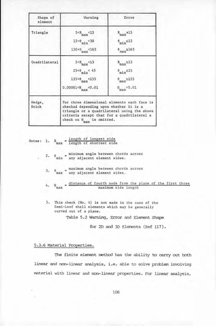
Sha pe of Warning Error e l ement

Triangle 5<R <15 R ~15 max max

15<6 i <30 m n 6 i :>15 m n

150<6 <165 6 ~165 max max

Quadrilat eral 5<R max <15 R ~15 max

25<6 i < 45 m n 6 1 ~25 m n

135<6 <155 6 ~155 max max

O.OOOOl<H <0 . 01 H >0. 01 max max

wedge, For three dimensiona l elements each face is Brick checked depending upon whe t her it is a

t r iangle or a quadrila t e ral using the above c r i t eria except that fo r a quadrilateral a

Notes:

check on H is omitted . max

1. R lenath of lon~est side max length of shortest side

2. 6 minimum angle between chords across =

min any adjacent element sides.

3 . 6 maximum angle between chords ac r oss max any adjacent element sides.

4 . H distance of fourth node from the pl ane of

max maximum side l ength

5 . This check (No. 4) is not made in the case of the Semi- Loof shell elements which may be generally curved out of a pl ane.

the

Table 5 . 2 Warning , Error and Element Shape

f or 2D and 3D Elerrents ( Ref 117 ) •

5 . 3 . 6 Mat eri a l Properties.

first three

The finite element method has the abil ity to carry out l:oth

linear and non-linear analysis, i.e . able to solve problem involving

material with linear and non-linear properties. For linear analysis ,

108

which is straightforv.ard, only the elastic m:Xlulus, Poisson' s ratio

and the density of the material must be specified (115, 117).

The solution of non-linear problems by the finite element

method is usually attempted by. one of three basic techinques:

(a) Incremental or step wise procedures;

(b) Iterative or Newton Methods;

(c) Step-iterative of •nixed procedure.

5.3.6.1 Incremental Procedure.

The basis of the incremental procedure is the s'tbdivision of

the load into many small partial loads or increments. The load is

applied one increment at a time, and during the application of each

increment, the displacement equations are c.tssumed to be linear. In

other words, a fixed value of the elastic stiffness matrix is c.tssumed

throughout each increment, but the elastic stiffness matrix. may take

different values during different load increments. The solution of

E;!aCh step of loading Ls ohrJ't Lr1ed as an increment of the d isplacements.

These displacement increments i:U"e a.c<~'..Jmulated to give the total displ­

acement at any stage of loading, and the incremental process is repea­

ted until the total load has been reached (112, 114).

5.3.6.2 Iterative Procedure.

The iterative procedure is a sequence of calculations in

which the structure is fully loaded in each iteration. Because sane

approximate constant value of stiffness is used in each step, equili­

brium is not necessarily satisfied. After each iteration, the r:ortiorl

of the total loading that is not balanced is calculated and used in

the next step to o::rnpute an additional increment of the displacements.

109

The process is repeated until equilibrium is apprmd..rrated (112, 114).

5. 3. 6. 3 Mixed Procedures.

The step-iteration or mixed procedure utilizes a combination

of the incremental and iterative schemes. Here the load is applied

incrementally, but after each increment successive iterations are

perfonned. The rrethod yields higher a=urr.~cy but at the price of rrore

a::rnputationr.~l effort (114).

5.3.6.4 COmparison of the Basic Procedures.

The principle advantage of the incremental procedure is ·its

complete generality. It is applicable to nearly all types of non­

linear behav to.ur. It provides a relatively a::rnplete description of the

load defonnation behaviour. Useful results can be obtained at each of

the intennediate states corresponding to an incremental of load. It

guarantees convergence to the exact solution. The incremental proce­

dure is usually rrore tirre consuming than the iterative technique and

it is difficult to knOIN in advance what increment of lOC!ds are necess­

ary to obtain a good approximation to the exact solution.

The iterative procedure is easier to program than the incre­

mental method and it is faster, provided it need analyse only a few

different loadings. The principle disadvantage of the iterative metho:J

i,; i:hili: t-Jv~re is no assurance that it will converge to an exact solut­

ion. The technique is not applicable to dynamic problems.

The mixed rrethod combines the . advantage of l:x:Jth the increme­

ntal and iterative procedures and tends to minimize r11e Jisa.dvantage

of each. Step-iteration is being utilized increasingly. The additional

a::rnputational effort is justified by the fact that the iteration of

110

the prcx::edure permits one to assess the quality of the approxirrate

equilibrium at each stage.

5.3.6.5 Non-Linear Analysis -PAFEC.

The PAFEC program uses the incremental prcx::edure to carry out

the non-linear analysis. The ITE.terial is assumed to behave elastically

before yield according to HCXJke' s Law. If the 1\"aterial is loaded

beyond yielding, additional plastic strain cx::curs, which if the load

is then removed, leaves a residual deformation. It is assumed that

data is available for the yield stress and stress-strain gradient

after yield for the case of uniaxial tension. Often the uniaxial stress

-strain curve will approximate to the ti/>,D straight lines of linear

elasticity and linear strain hardening after yielding, so that it is

defined by the elastic modulus, the yield stress, and the plastic

stress-strain gradient.

5.3. 7 Loadings.

These ITE.y consist of point loads applied at the node or

pressure loading applied over a plane enclosed by a set of nodes. A

constant or varying pressure load can be applied over one surface of a

3D brick element and the program then converts the pressure load into

equivalent nodal loads. The ITE.gnitude of the nooal forces is determin­

ed by interp:>lating between the nodes that are enclosed within the

area of the pressure. Fig 5.3 shows the equivalent nodal forces for a

given pressure applied on the surface of the rrost a::mronly used eleme­

nts. Detailed calculation of the equivalent nodal force is illustrated

in Appendix r.

111

l 12

Note: (i) Total uniform load applied over the element = 1:

(ii) + ve = inwards, and - ve = outwards.

Fig 5.3 Equivalent Nodal I..oads due to Constant Pressures

on Element Surface (Ref 117).

5.4 Three Dimensional Pavement Model.

2D analysis requires less cx:::mp.1ting ti.rre, disc space and a

smaller base ( cx::mp.1ter merrory) than a 3D analysis • 2D analysis of the

pavement rcodel using the PAFEC program was carried out at the Plyrrouth

Polytechnic by Butler (13). The pavement was rcodelled to predict the

surface deflection in the wheel path under the loading action of a

Deflectograph (18). Hov.ever the stress on each element of material

varies in three directions when subjected to a load. In addition, the

deflection treasured by the Deflectograph is relative to a datum of the

T-frarre which has one of its supports off the line of the wheel path.

The layout of the Deflectograph asseroly is given in Plate 2.1, Figs

2. 3 and 5 .4. The deflection profile along the road through the centre

of the twin rear wheels ( line XX en Fig 5. 4) and the centre line of

the vehicle along which the T-frarre noves ( line Y'f en Fig 5 • 4) is

illustrated in Fig 5. 5.

112

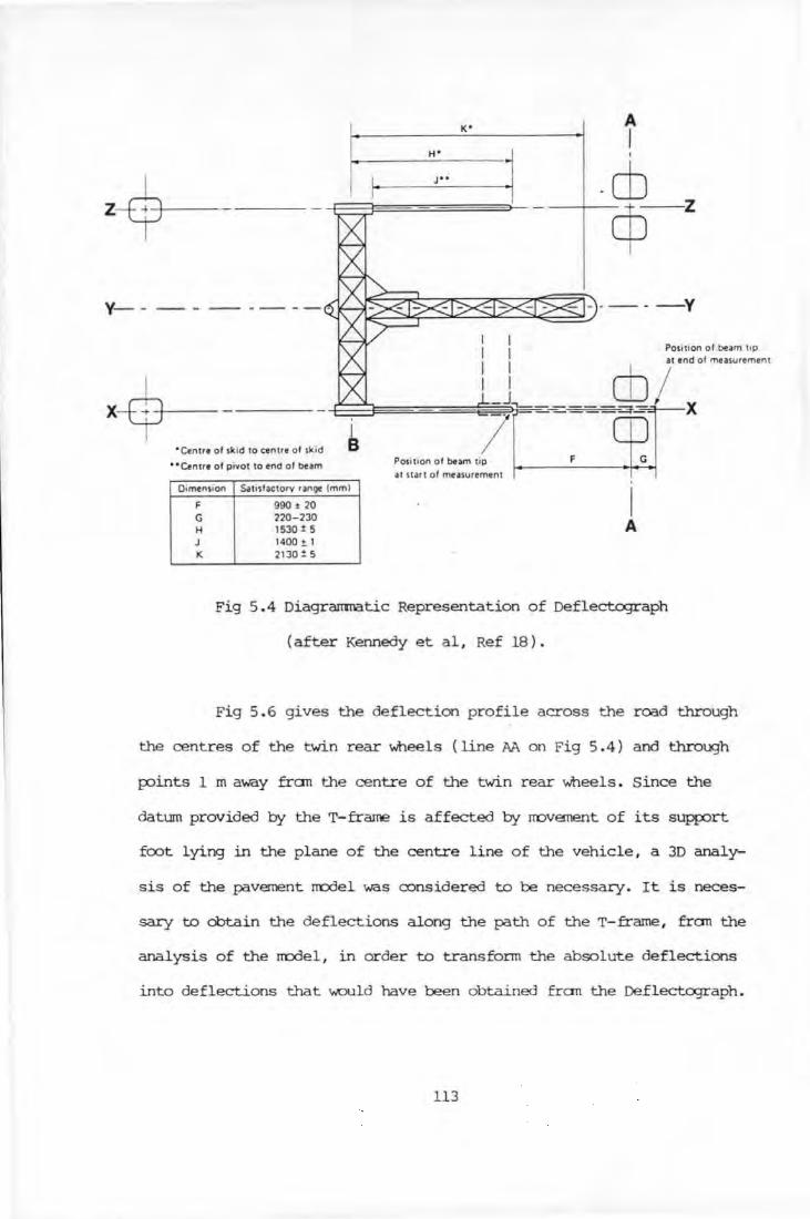
I z-?--

V- - ------- -

'Centre of skid to centre of sk id

"Centre of pivot to end of beam

' I B

Dimension Satisfactory ran~ (mm)

F 990 .t 20 G 220-230 H 1530 ! 5 J 1400!. 1 K 2130!5

K'

H'

I I I I I

_j:-l-

7 Posouon of beam tip at start of measurement

A I I

cb ---+-- -t --z

cp -----Y

F G

I A

Fig 5.4 Diagrammatic Representation of Deflectograph

(after Kennedy et al, Re£ 18 ) •

Fig 5 . 6 gives the deflection profile across the road through

the centres of the twin rear ...meels (line M on Fig 5 .4) and through

_I:Oints 1 m away fran the centre of the twin rear ...meels . Since the

datum prov ided by the T-frame is affected by rrovernent of its SupfOrt

fCX)t lying in the plane of the centre line of the vehicle, a 3D analy-

sis of the pavement rrodel was considered to be necessary. It is neces-

sary to obtain the deflections along the path of the T-frame, fran the

analysis of the rrodel, in order to transform the absolute deflections

into deflections that would have been obtained fran the Deflectograph.

113

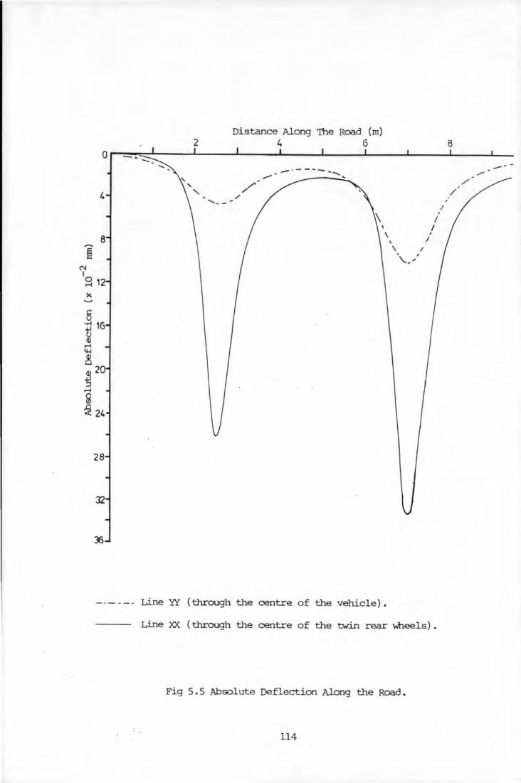
Distance Along The Road (m) 2 4 6

/ ......... _-"'

, I

I \ '

\ / \ /

Line YY (through the centre of the vehicle) •

Line XX (through the centre of the twin rear wheels) •

Fig 5.5 Absolute Deflection Along the Road .

114

8

--/

/ I

In order to develop a realistic 3D rrodel, a number of initial

rrcdels were developed and there are detailed in the next few sections .

These initial rrcdels were intended to provide information on the shape

of tyre area, type of elements, number of element, geanetric dimens-

ion, accuracy, a::rnp.xting time, base, disc space required and on the

type of restraint and loading to be used.

Undeflected Surface

----- ---- ..... - . - ---------

- 1 m away fran the centre of the twin rear Wheels

Through the centre of the twin rear Wheels (line AA eo

Fig 5 .4).

Fig 5.6 Deflection Profiles Across the Road.

5 .4.1 Mcdel A.

The aim of this rrodel was to choose the rrost sui table shape

of the tyre contact area with the road. The shape of the tyre contact

area is oot circular or rectangular but rrore elliptical as shown in

Fig 5. 7 (18). Research (26, 120) into the shape of the contact area

suggests that it is .r:ossible to assume a circular shape of area equal

to the load, 'W', carried by the tyre divided by the Pressure (P) of

the Wheel (see A~dix II), i.e.

Area (A) = W/P (5.2)

115

The radius of the circle could be deduced fran fran the area. Fran the

details of the Deflectograph given in LR 834 (18), the radius was

found to be in the range bet.....een 77 to 94 nm, but for convenience the

radius was assumed to be 100 nm. There are two methods of incorp:>rat-

ing the circular area into the program:

(a) Divide the circular area into a number of tr~angles with one side

curved. This rnethoo involves allocating a mid-node on the curved

surface. During the analysis process, the curved surfaces are

divided into a number of small triangles as shown ~n Fig 5.8a.

This method is very tedious and req1..1ires a great anount of data to

be input.

(b) The process adopted divides the circular area into a number of

straight sided triangles as shown in Fig 5 .8b. This method is very

much simpler and straightforward; It requires a small~r ~n~unt of

data to be input and toth methods offer rrore or less the same

accuracy ( 116 ) •

The area of circle can easily be approximated by the use of

the inscribing and circumscribing p:>lygons. The p:>lygons are divided

into triangles each with a vertex at the centre of the circle. It is

then a simple matter to evaluate the sum of the area of all the trian-

gles. It is also p:>ssible to approximate the circle with tri'l.n':Jl~,o;,

u1e lengths of which when summed provides a good approximation to the

perimeter of the circles. Since pressure wouln be applied over a

circular area, it is better to approximate the circle by triangles of

equal area.

The circular area was split into 8 equal isosceles triangles,

h d. 0 . .

eac subten 1.ng 45 at the centrr'! •)f l:he c1rcl8 a:~ slxxm ln F'ig

5 .:Jb. It •:n.s cl<'!cided to use a maximum of 8 triangles inscribing the

116

circle since a greater number will increase the number of elements

which in turn will increase the file, base size and the comp.1ting time

Model A was constructei ~nd three loading cases were conside-

red:

(a) Pressure load over 8 e::JUal isosceles triangles;

(b) Pressure load over 4 e::JUal squares;

(c) Single Point load at the centre.

The rrodel consist of one layer only. The value of the elastic nodulus

is irrevelant at this stage, provided that the value used was the same

for all the loading cases. At this p::>int, the load case No (a) vas

assumed to be the correct one and remaining two cases were ccmpared

with load case No (a) ._Fran the comparison of the results, case No (b)

was found to be similar to case No (a). It was concluded that initial­

ly eight equal isosceles triangles would be used but if any problems

were encountered with the disc space or the oanp.1ting time required,

then the four equal square shape would be used.

5 .4. 2 Model B.

The main purp::>se of constructing this rrodel was to get an

estimation of the necessary dimensions of the model and to study the

effects of the nearside front wheel and the offside twin rear wheels,

OS, (away fran the kerb) on the deflection profile along the centre

line of the vehicle and centre line of the nearside twin rear wheels,

NS, (close to the kerb) .The definition of the centre line of the

vehicle (line YY) and centre line through the twin rear wheels, near­

side wheel path (line XX) and offside wheel path (line ZZ) are illust­

rated in Fig 5.4. It would be very difficult to rrodel the front wheels

and two sets of twin rear wheels together since this would require an

117

enorm::>us am:::>tmt of cx:mp.lting resources. Therefore, it is crucial to

know if is fX>ssible to exclooe the nearside front am/ or the offside

twin rear wheels, in the final m:::x:3el, see Fig 5.9.

160-190

Fig 5.7 Deflect.ograph

Tyre Print ( Ref 18 ) .

(a) Curve Sides (b) Straight Sides

Fig 5. 8 Triangles with: (a) Curve Sides

and (b) Straight Sides.

~el Bl was constructed and the dimension of the m:::x:3el are

as s'hor.Nn in Fig 5 • 9a. The deflection along the lines XX and YY (see

Fig 5 • 9 ) ....ere recorded for the two loading cases :

(a) ~ sets of twin rear wheels, NS (nearside), OS (offside), see

Fig 5 • 9, loaded together,

(b) Twin Rear wheels, OS, loaded alone.

Fran these two load case it is };X)ssible to determine the effect of the

twin rear wheels, OS, on the deflection profile along lines XX and yy.

The result indicates that the twin rear wheels, OS, do affect the

deflection profile along OOth the lines XX and YY.

118

(a) M:Xlel Bl

\

\

E E

0

~ z F-·- - -·- · --

y ---------

Oos -· ----- ·-·z Oos ________ __ _ y

E E

If)

oX ONS ~------·-· _____________ x_

ONs

2475mm 1875mm

\

' .__ ___ _jJD---x

(b) M:Xlel B2

E E

U")

0

:?:.._ ____ _ 0 ------- ·- · - - - · ---~

0 y ~--- -------- ---------- - - - - - - --- --- _Y

E E

If)

o ~--------·-·-·-Q X 0 . ---- ____ -:..:.. E E

~

21.75mm 187Smm

Fig 5 .9 Model Bl - B2.

119

Mcx:'lel B2 was constructed, as shown in Fig 5 • 9b, with the

dimension in the z direction decreased by 750 mn. The deflection along

the lines )0( and YY was recorded and a::mpared with those obtained fran

Mcx:'lel Bl. There was no significant change in the deflection.

Therefore, it is possible to limit the width of the rrodel in the z

direction to 3830 mn and restrain it in the z direction.

Model B3 consists of one front wheel and twin rear wheels,

NS, as shown in Fig 5.10a. Two loading cases were considered:

(a) Front and twin rear wheels, NS, loaded together;

(b) Front wheel'loaded alone.

Fran these load cases it is possible to detennine the effects of the

front wheel on the deflections along the line )0(. The deflections

generated along the line XX usi11g this rrodel were oanpared with those

obtained fran MOOel Bl. Fran the results it o:mld be deduced that the

front wheel affects the deflection along the lines )0( to a distance

al:out 2 m away fran the centr"! of the twin rear wheels, NS. The twin

rear ..meels, OS, have a greater effect on the deflections along the

line )0( than the front ..meel.

'l'he length of the rrodel, in x direction, was then reduced:

first the distance in front of the front ..meel, s<'!e Mooel B4 in Fig

5.10b, and secondly the length both in front of the front ..meel and t.n

the rear of the twin rear ..meels, see Mooel B5 in Fig 5.10c. 'l'he defl­

ection along thP. li11e )0( fran both rrodels were oanpared with those

obtained fran Model B3. 'l'here were no significant changes in the defl­

ections.

120

E E lf)

c;

'··-· 8 0 X -·- - - - · - · - · - · - · - · -·--- · -·- · ---·-:;..

0

2500mm L.SQ;)mm 3Q))mm

E E ~

E E

§ r-

E E lf) r-Gl

E E 8 0 .-

(a) M:Xlel B3

0 -- - · - · ------.X

0 !_ -8----------

1 1CXX>mm 1 L.500mm 3<XX)mm

(b) M:Xlel B4

X.- -G-- -- --- 0 X ---------- - -·..:

1 1000mn1

\ . .

0

L.SOOmm 18JJmm

(c) M:Xlel BS

Fig 5.10 Models B3 - B4.

r.------· o-x

121

All the alx>ve Models, Bl to B5, consist of two layers of

total thickness 680 mn. Each !TDdel was nm twice with different elast-

8 9 2 ic !TDdulus for the upper layer; 1.5 JC 10 and 5 JC 10 N/m rut

the same Poisson's ratio of 0.35. In ooth cases, the lo....er layer had

the same elastic !TDdulus. In all these !TDdels, the front and rear

5 2 wheels loads were input as a pressure load of 6.9 JC 10 N/m • The

contact area of the tyre was represented by eight equal isosceles

triangles as shown in Fig 5.8b. Twenty noded brick elements and fift­

een noded wedge elements were used • The ooundary conditions of the

models are as follows:

~-lOdel Plane Direction Restrained

131 t..o 85 ABCD JC, y, z

AECG JC, z

BFDH JC, y

crx:;H JC, z

ABEF JC, z

Table 5. 3 Boundary conditions of Model B.

5.4.3 Conclusions to be Drawn fran The Initial Models A-B.

Analysis of the above models leads to the following conclus-

ions:

(a) The front wheel affects the deflection along the line XX to a

distance alx>ut 2 m.

(b) The front wheel could not be excluded fran the final model even

though it only affects the deflection to a dist.nnce about 2 m,

since in order to get a Deflectograpl1 deflection over a meter, the

122

measuring ann should be at least 2.54 m away fran the centre of

the twin rear wheels (see Fig 5. 4, Point A is alx:>ut 2. 54 m away

fran Point B) •

(c) The twin rear wheels, OS, affects the deflection along the lines

XX and YY.

(d) The twin rear wheels, NS, have a greater influence on the

deflection along the line XX than the front wheel. This ':'Ould be

di.E to the fact that the twin rear wheels loads are twice the

ll'BJnitude of the front wheel load and also they are closer to the

twin rear wheels, NS.

(e) The distance in front of the front wheel could be reduced to

1 m and in the rear of the twin rear wheels to alx:>ut 1.5 m.

(f) If the front and the twin rear wheels, OS, could not be acCO'llli'Cd­

ated together in the final model, then the front wheel woulci have

to be eJCcluded. (In the final model only the front wheel and the

twin rear wheels, NS, were used, see Section 5. 4. 7) •

5.4.4 Model c.

The main pllr!X)Se of constructing this model was to find a

method of including the effect of the twin rear wheels, OS, on deflec­

tion along the lines XX and YY, but without including the wheels in

the final model, since this woulc'l re<'luce the size of the model and the

canp.~ting time and the disc space associated with it. The Model Cl,

whose dimension is based on conclusions stated in Section 5.4.3, was

cut along the line of synmetry, i.t'!. line YY, see Fig 5.lla, to a

model, Model C2, as shown in Fig 5.llb. In these two models, the tyre

contact area was represented by a square ( 100 rrm x 100 mn) instead of

8 equal isosceles triangles, since the 8 isosceles triangles require

123

greater a::mp..~ter resources with no improvement in accuracy. The effect

on the shape of deflection profile by this chi'inge was studied. Both

fonns of contact area gave the same maximum deflection. 'I'he deflect­

ions at sane distance away fran the point of maximum deflection were

greater for the triangular shape a::mpared to the square shape, by

arout 3 to 6%. '!Wenty noded brick elements were only used for the

entire construction of Mo::lel Cl and C2. The rrodel consists of two

layers of total thickness 680 nrn with the same elastic rrodulus of

1.5 x 109

N/m2

• The plane of the rrodel was restrained as shown in

Fig 5 .11 • The deflections along the lines XX and YY fran Model Cl and

C2 were a::mpared and the following conclusions were deduced:

(a) The deflection along the lines XX and YY for b:>th rrodel were

very similar, within engineering limits, al::out 4%.

(b) The ~ting time and disc space required for Model C2 was half

of that required for Model Cl.

(c) The number of elements, oomputing time and disc space required for

a square contact area was much less compared to the triangular

area.

The b:>undary conditions of Mo::lel Cl and C2 are listed in Table 5.4.

5.4.5 Mo::lel D.

Using the results fran Mo::lel C2, it is possible to exclude

the twin rear wheels, OS, without excluding its effect in the final

rrodel. This made it possible to include the front wheel as shown in

Model Dl, see Fig 5 .12a. The main purpose of constructing Model D was

to find a means of dividing the Mo::lel Dl, into two separate rrodels,

Model 02 and 03 (see Fig 5.12), then to analyse the two rrodels separa­

tely and finally to superimpose the deflection, along the lines XX and

124

------------------------------------------------------------------ ------

YY, by using the Principle of Superposition.

Plane Direction Restrained

ABCD x,y,z

ACGE X

BFDH X

CGDH z

ABEF z

Table 5.4 Boundary Conditions of Model Cl and C2.

From oeflection profiles obtained from TRRL experimental

sections of roads loaded with a Deflectograph !lOving at creep speed,

Figs 5.13 and 5.14, it can be seen that the deflection due to front

wheel is negligible at a distance of about 2. 5 m frc::rn the centre of.

the front wheel (Point P in Figs 5.13 and 5.14). Therefore, the m:xlels

were superimposed over a distance of 3 m between the front wheel and

the twin rear wheels, NS, as shown in Fig 5 .12. The deflection along

the lines XX and Y'l from Model 02 and D3 were superimr:osed and compar­

ed with those obtained from Model 01. The comparison was carried out.

for different OJI11binations of restri'!.int applied to plane BDFE. The

deflections were not found to be similar and therefore it is not r:oss­

ible to divide the Model Dl into Model D2 and Model 03. The thickness,

number of layers, tyre contact arP.A a.nd elastic modulus of the Models

D were similar to Models C.

125

5.4.6 Model E.

l't:ldel E was cnnstructed in order to determine the geometric

dimension and the type of elements to be used in the final rrodel.

During the operation of the Deflectograph (18), the datum T-frame

projects alx>ut 6\JO rrrn beyond the centre line of the twin rear wheels.

The deflection profile illustrated in Figs 5 .13 and 5 .14 indicates

that the absolute deflections along line YY, see Fig 5 .12, on either

side centre of the wheels are the sarre for a distance of 600 mn.

Therefore, it is possible to rrodel only half of the twin rear wheels

as shown in Model E, see Fig 5 .15, and use the deflection at 600 mn in

front of the twin rear wheels as equal to the deflection at 600 mn

behind the wheels.

It is cnstly to use 20 n:Xled brick elements for rt l~rg~ 3D

rrodel and therefore it would be ecnnamical to use only 8 noded brick

elemP..nts. The same accuracy cnuld be achieved to a certain extent by

using a finer mesh neac the loaded zone and a cnarse mesh for the zone

away from the loaded zone. Figs 5.15 ;md 5.16 give the detail descrip­

tion of Model E, which consist of eight layers. Each layer can have

different material properties, but all the sub-Layers within each main

Layer must have the same material properties.

126

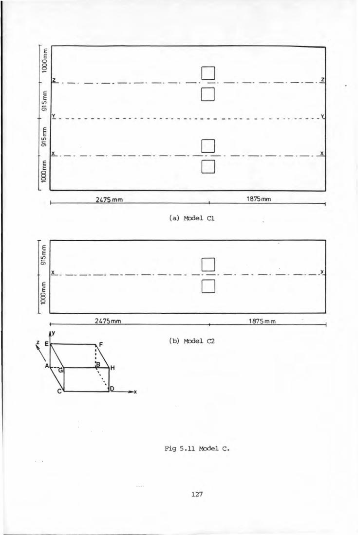
E E

0

8

E E

§ r-

E E

lf)

Ci

E E

§

0 -- -- - - ---- - ---- - ~ L ________ ____ __ _

0 y --------- _____ v

0 - - - - --- - - - ----- - --~ x_ ___ - - -- --- - - -

0

2475 mm 187Smm

(a) l't:Xlel Cl

0 --------- - - - - - - _ _ )I

.!._ _________ _ _ _ _ ___ _

y

2475mm

. . ~--------~D~~·x

0

1875mm

(b) l't:>del C2

Fig 5.11 Model C.

127

~ ~

u..__ -- -o-r,.- ---

1CXX! rrm 4SQQmm

(a) M:xJe1 Dl

B G

\

' ' ' --------------~F--~-x

1000rrrn 1 3000mn

2SOO mm

-

D ---- - _x

0

1850mm

(b) M:xJe1 D2

~~----~---------

(c) M:xJe1 D3

1/)

o; I D ---- - - - . -~ - . --I - -------

1 D I

~- ---- · - - - · -

: 3Smmm 1850mm

Fig 5.12 t-bde1 D.

128

-§ N I 0 ....-!

X

c 0

·.-t

t Ql

....-! ~

~ Ql

~ ....-! @ ~

8

12

16

20

21.

2 Distance Along The Road (m)

........ _- ...

/' /

/

I. 6

\ /

\ I

Line Y'f (through the centre of the vehicle) •

8

Line )Q( (through the centre of the twin rear wheels).

100 mn Ibt Rolled Asphalt

300 mn Wet mix Macadam

150 mn Type 2 Sub-base

Fig 5.13 Absolute Deflection of The Granular Roadbase Pavement.

129

Distance Along The Road (m)

7 8

2 /

/

I I

l. I

1 /

N I 0

G ~

X -§ ·ri .., {)

8 Q) ~ 4-4

8 \

Q)

~ 10

rl

~ ~ 12

1!.

1G

----- · Line Y'i (through the centre of the vehicle).

Line XX (through the centre of the twin rear wheels) •

lOO mn fbt Rolled Asphalt

75 mn Dense Tarrnacadamn

150 mn Type 2 Sub-base

Fig 5.14 Absolute Deflection of The Bituminous Roadbase Pavement.

130

...... w ......

Plane Direction

Restrained

AOCD X, y, z

ABEF z

G I I I I

I

--.-- - - .-- . ----- -- - --- - L --cr:GH z I

I ACEf], z c - - - - - - - - - - - - - - - - - - - - - - - - - - - - - - - - - - - - - - ~D BIHF z

TOtal Nodes: 2594

Total Elements: 2096

TOtal Degree of

Freedan 6325

Ccmp.lting Tirre: 10,666

Element Type: 37100 -8 Noded Brick Element

37200 -6 Noded Wedge Element

Fig 5.15 3D View of Model E.

'

4500 mm

' ' ' ' ' \ \

' \ (X)

' -\ 0 \

'

\

~

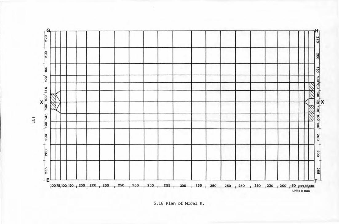
0 N N

0 0 N

0 U') .,..

0 0 .,..

0 0 --X-:-

o 0 .,.. U') ..... .,

w N 0

0 .,..

0 0 N

0 0 N

U') U') N

E

V ~ 1\ ~ j

r--.....

~00,]5 110<lt 150 I 200 I 220 250 250 250 I 250 I 255 300 I 255 I 250 I 250

5 . 16 Plan of Model E.

~ 0

N 0 0

.... ~ .... 0 0

~ .... 0 0

~ .... 0

~ 0

1/ - ID

r'- -o

~ .... 0 0

K-

~ .... ~ 8 N 0 0

N 0 0

N (JI (JI

F 250

Units= mm

When the rrodel was analysed using appropriate but approximate

elastic noduli values for each layer, the deflection at the centre

point between the front and twin rear wheels was quite small. The sur-

face at this !X)int was deflecting up...rards ( + ve deflection) rather

than deflecting downward (-ve deflection). AC<Drding to Desai et al

( 114 ) , if the structure is symnetrical, the thickness V ( see Fig 5 .17 )

should be least 10 to 12 t:i.roes greater than D, the diameter of the

wheel. The distance H should be at least 4 to 6 t:i.roes greater than the

dialreter D. The distance H and D are the critical distance beyond

which the l::otmdary a:mditions have a negligible effect oo the surface

deflection profile.

plane or axis of symmetry

Fig 5.17 Finite Representation of Infinite Bodies

(Desai et al, Ref 114).

5.4.7 Model F. to

Model F was a:>nstructed in ardedina:>rp::>rate Desai et al

r . (113) suggestions. Therefore Model E was reaJnsttPcted Wl. th 9 layers

instead of 8, i.e. the subgrade thickness was increased to 2.244 mn,

to give Model F (see Fig 5.18 and 5.19). The distance between the

centre of the twin rear wheels and the kerb l::otmdary (plane EFAB in

133

Fig 5 .16), was increased to 1. 3 m. When the JTCldel was analysed with

elastic JTCldulus similar to Model E, the deflection between the twin

rear wheels increased by .15% but the deflection at the centre point

be'bNeen the front and the twin rear wheels increased by 200%. To

reduce the a::mputing time due to the increase in the number of layers,

the manner of division of the model into a number of finite elements

was changed. The dimension of the tyre cnntact area was changed fran

100 nm square to 85 nm square and the distance be'bNeen the wall of the

twin rear wheels was increased fran 90 nm to 150 nm so that the dimen-

sions are rrore in accnrdance with those stated in Ref ( 18) • These

changes in the dimension of the contact area and the distance betv.een

the walls of the twin rear wheels did not produce a significant effect

on the deflect ion profile. This change enables the deflection at

centre of the twin rear wheels I r:oint ' a' in Fig 5 .18 I to be obtained

unlike the case with Model E in Fig 5 .16.

The plane BDHF and ACEG, see Fig 5 .18, was restrained fran

rroving in the x direction, since the deflection for a distance of 1 m

on either side of the line HF is symnetrical. The plane crx:;H was rest-

rained fran rroving in the z direction, since the deflections are symne-

trical about the line GH. Total restraint (in x, y, z direction) ...as

applied to the lov.er plane ABCD to represent the bedrock surface. The

plane ABEF was not restrained in any direction. The plane ABEF repres-

ents the interface between the pavement and the soil. In practice,

there will be a very partial restraint on the plane in all three

directions and this restraint will increase with depth. Ideally sane

sort of spring 1nechanism with increasing stiffness with depth at the

interface between the pavement and the soil could be used to model

this effect. Since this suggestion could not be implemented easily

1 ' ' - _-:.~

with the PAFEC program, the plane (ABEF) was treated as a free plane.

The l:x:lt.mdary conditions and the number of elements used are surnnarized

in Tables 5.5 and 5.6. It is possible to divide each layer into a

number of sub-layers. The thickness of each sub-layer must be within

the range specified in Fig 5.19. Each layer can have different materi­

al properties but all the sub-layers within each of· the main layers

must have the same material properties. The PAFEC program for this

'rodel is shown in AfPE!I"ldix III.

Plane Direction Restrained

ABCD x, y, z

.li.BEF FREE

cr.GH z

ACEG X

Ba-IF X

Table 5.5 Bot.mdary Conditions of-Model F.

Total tbdes 2920

Total Elements 2331

Total Degrees of Freedan 7434

Element Types 37100 (8 Noded Brick Elerrent)

37200 (6 Noded Wedge Element)

Table 5. 6 General In formation ab:mt Model F.

135

...... w 0'1

r.

0 CO N

0 I()

0 CD

I()

CO -X .,

CO

0 CD -0 I()

0 I() N

0 -.., I()

'<t ..,

E

~ :/ '\

~ V ~

p517S}OQ1 160 1 200 1 220 1 250 1 250 , 250 I 250 I 260 1 300 I 260 I 250

5 .18 Plan of Mcx:lel F.

P,: ~ 11 In

\ ? /:

011

"'

N

"' 0

F 250 1 250 I 250 1 220 1 200

1160 ,10Q, Z!i,B!j

Units= mm

1a5?5'o<lt 160, 200 1 220 1 250 1 250 1 250 1 250 1 260 1

3oo 1 260 1

250 1

250 1

250 , 250 1

2201

200 1160 ,10~1~~

H1 - H9 = 75 to 374 mm Units= mm

Fig 5 .19 Various Layers of Model F. F

a---x

5.5 Validation of The Final Model (Model F).

Before the rrodel could be used to investigate the relation­

ship between the deflected shape and the pavement condition, it was

necessary to ensure that its res~nse was similar to that of an actual

pavement structure. Absolute deflection recorded by in-situ displace­

ment transducers, inserted into an experimental pavement with a granu­

lar road base, have been used to define the pavement res~nse to be

rrodelled. These measurements were carried out by the TRRL under the

loading action of a Deflectograph.

5. 5 .1 Granular Road Base Pavement.

The pavement with a granular road base was represented by the

layered system as shown in Fig 5.20. The only infonnation available

al::out the parameters controlling the res~nse of each layer is the

thickness of the surfacing, road base and sub-base. The other infonna­

tion available are the loads of the front and the twin rear wheels.

The temperature of the environment at the time of measurement of the

deflection was not available. In developing the rrodel, the elastic

rrodulus and the Poisson' s ratio of each layer of the pavement layers

and subgrade were initally deduced from typical published values for

each material type. These values were subsequently rrodified until the

res~nse of the theo&ical rrodel was similar to that of the actual

pavement structure.

138

Asphalt Bound Layer, E1 , H1 , /L1

Intemediate Granular Layer, E2, H2

, /L2

Fig 5.20 Granular Road Base Pavement.

5.5.1.1 Subgrade layer.

The response of the subgrade was controlled by the resilient

(E ) I s

Poisson' s ratio IL3

and the limiting thickness

H3

• According to Desai et al (ll4), the depth of the whole structure

should be at least 10 or 12 times the diameter (170 rrm) of t."'le wheel.

Since the pavement thickness was about 550 rrm, the thickness of the

subgrade was fixed to 2250 rrm. This will ensure that the lov.er round-

ary condition will not have a significant effect on the surface defle-

ction profile.

It has been reported (56) that the subgrade soil is stress

dependent and relationships have been developed between stress, strain

and rrodulus. Hov.ever, Bleyenberg et al ( 121) , have derronstrated fran

full scale road experiments, that linear elastic theory may be used to

describe the p;lVement response, provided that the mxlul i of the mater-

ial were detemined fran appropriate loading conditions. Where in-situ

measured subgrade modulus is not available, the empirical relationship

betv.een dynamic subgrade modulus and the CBR value may be used (ll5):

7 2 E = 10 x CBR N/m (5.3) s

The subgrade mxlulus for the granular road base pavement was not

139

available, but based on the knowledge of the soil type, a CBR 15% was

chosen as an appropriate value at the formation level and these give a

7 2 subgrade rrodulus of E3 = 15 x 10 N/m . The subgrade rrodulus was

- 7 2 assumed to vary linearly fran 15 x 10 N/m at the formation level

to 100 x 10 7 N/m2 at 2. 25 m below the formation level. The Poiss-

on's ratio, ~3 , was assumed to be 0.35.

5.5.1.2 Intermediate Granular Layer.

The rrodulus of the unbound base layer is to a large extent

stress dependent (122). ·Theoretical analysis and field measurements

have shown that the modulus of the unbound base layer, E2

, depends

on its thickness H2

, and the modulus of the underlying subgrade,

E3

, according to the following relationship (43):

8 2 =·~ E3 (5 .4)

where 'S = 0.2 H2

with H2

in rnn, with the limit 2< K2

<4.

An initial value of E2

= 2 x 108 N/m2 was assumed for the ccmbi-

nation of the wet mix macadam base and type 2 sub-base. The Poisson' s

ratio, !J?.• was assumed to be 0.35. The thickness of the granular

layer, H2

= 450 mm, was split into two layers of 300 mm and 150 mm

for analysis. '!'his enables different modulus values to be assigned to

the wet mix macadam base and the type 2 sub-base layer if required.

5.5.1.3 The Asphalt Bound Layer.

The stiffness modulus of the asphalt mix can vary considera­

bly fran around 1 x 107

to about 5 x 1010 N/m2 . The upper range

of stiffness values (say l ~ 10 g to 5 x 109 N/m2 ) has been

determined for a large number of asphalt mixes by means of dynamic

and/or semi-static (e.g, constant rate of loading) test at various

140

temperature and under different loading conditions. The rrodulus is

dependent solely on the bitumen content, the stiffness of the bitumen

and the voids in the mix. The stiffness of bitumen which varies with

loading time and temperature can be estimated with the aid of Van der

Poel' s nanograph (41). The loading time was detennined using following

equation ( 42 ) :

-4 log t = 5 x 10 H - 0.2 - 0.94 log V (5.5)

For the pavement considered, H = 150 mn, and V = 2 Krn/hr and therefore

the loading time, t = 0.36 secs.

A 50 pen grade bitumen was assumed. Properties of the binder

for typical mixes and the properties of HRA wearing course were obtai-

ned fran Tables 2 and 3 of Ref ( 42) •

pi =50

Pr = 0.65 Pi= 32.5

SPr = 98.4- 26.35 log Pr = 58.6 °c PI = 1951.4- 500logPr- 20SPr

r 50logP - SP - 120.14 r r

= 0.2

(5.6)

(5.7)

(5 .8)

( 5. 9)

It was reported (123) that the temperature (T) vas low when the measu-

0 rements were taken ;md therefore 10 C was assumed.

0 SPr- T = 48.6 C (5.10)

Using the Van der Poel' s nanograph (41), Fig 3. 2, ~ (stiffness of

bitumen) is equal to 200 MPa.

VMA =V +V = 21.6% B V

('5.12)

Using the relationship between mix stiffness (Sm)' binder stiffness

141

( ~) and VMA in Fig 5. 22 ( 41 ) , the mix stiffness is equal to

6 x 109

N/m2

• Therefore, the rrcdulus of the asphalt round layer

was first assumed initially be 6 x 109

N/m2 •

50

f--- -

10 0 ~-

0... Q 5 (f) (f) w z LL lL 1-(f)

X ~

0·5

0·1 1

. - - -~ . -· ·- -·---- - I- - - .

~ ~~ V - -- r-- - - -

vv I

~ I V I / L-v V 1-

i:Z-' VM~%) f / L ~ V/

12

11.

16 18

20 22 21. 26 28 30

I

/ - V // V V v lA ./ ./

v!.-- / / v " j ~V~ L']/ y v~ t::/ / k'

~/ -: V ?i ~.-)"

, , ~ ,/ V I / / ,.-:

r-1-

~P'~ ~~ ?L 1--

-1 - 1--- z:

~ v 77 --

V / · - --V V

1--· Vv~-' ~ -r---- - -·

5 10 50 100 BITLMEN STIFFNESS (MPa)

S S [l 257.5 - 2.5 VM~ l" m • b + n(VMA - 3) j

(4 X 10

4) n • 0.83 log -

5-b

_.I-

~ 1---vv r--~--' v I----~

~ Vv v~-" V 1-.Y ~V V ~

/'[ / / V A'/ / 1/// V./

:

11

500

Fig 5 . 21 The Relationship Between Mix Stiffness, Binder Stiffness

and VMA ( after BrOINO. et al , Re£ 42 ) •

142

5.5.2 Matching The Response of The 3D Model and Actual Pavement

Structure.

The elastic rrcdulus, Poisson' s ratio and the thickness of

initial rrcdel are given in Fig 5. 22. The front wheel load is 22 KN and

the rear wheel load is 17 KN. When the rrcdel was analyzed using the

values, the maximun deflection obtained was less than the actual

value. The deflection at a distance 1 m away fran the point of maxi.nu.nn

deflection was positive instead of negative, i.e. surface deflecting

up..oards. This shows that the subgrade value assumed is very stiff and

therefore the elastic rrcdulus of the subgrade was la...ered to CBR 10%

at the surface of the subgrade. The rrcdel was then analyzed with the

subgrade rrcdulus varying linearly fran 1 x 108

N/m2

at the surface

to 1 x 1010

N/m2

at the base of the subgrade layer. This very much

increases the deflection, l:oth at the point of maximum deflection and

at a distance 1 m away fran the point of max:imun deflection, t.cllo.ards

the actual value.

9 2 El = 6 X 10 N/m , Jl.l = 0.35,

1"2 = 0.35,

fi.:J = 0.35, H3

= 150 nm

E4

= Varied linearly with depth fran 15 X 10

8 2 to 10 X 10 N/m , p.

4 = 0.35, H

4 = 2245 mn

Fig 5.22 Elastic Modulus, Poisson's Ratio and

The Thickness of the Initial Model.

The rrcdulus of the subgrade at various depths was also alter-

ed so that it is no longer follows a linear variation with depth.

Change in rrcdulus values at various depths, affects the shape of the

143

deflection profile at sane distance, say 500 to 800 mn, away from the

point of r:naJCimum deflection. The final values of the subgrade rrodulus

at various depths is shown in Figs 5.23 and 5.24. Figs 5.25 and 5.26

shows the deflection profile, along the centre line through the twin

rear wheels, Fig 5. 25 ( line XX of Fig 5. 4) , and along the centre line

of the vehicle, Fig 5. 26 ( line YY of Fig 5. 4) , obtained from the 3D

finite element rrodel and those obtained by the TRRL. Fig 5. 27 shows

the Deflectograph deflection profile for the in-situ pavement struct­

ure, and the profile a Deflectograph would see if measuring the defle­

cted shape generated by the 3D finite element rrodel. Those figures

show that deflection profile, l::x:lth absolute and l)eflectograph, for the

actual pavement and the rrodel are very similar for the first 1. 5 m

away from the point of r:naJCimum deflection. Beyond the 1. 5 m, the canp­

uted deflectiors are less than the actual deflection and this could be

due to the coarse mesh size around the front wheel. Full details of

the effect of Change of the elastic rrodulus of the various layers, on

the deflection profile is discussed in Chapter 6.0.

5.5.3 Comparison Of Asphalt Tensile Stresses.

The Shell method (124) presents a procedure for calculating

the average stress levels in the bituminous layer. The bituminous

layer is first divided into three sub-layers: the first two layers

should be 40 nm thick and the third iayer equal to the total hi tumin­

ous layer thickness less 80 nm. The bituminous layer is subdivided so

that the temperature at different depths can be taken into account. It

is based on detr.J.iled studies (124), from which it has been concluded

that the upperrrost layers are subjected to the greatest temperature

changes and are usually made of different types of mix from that used

144

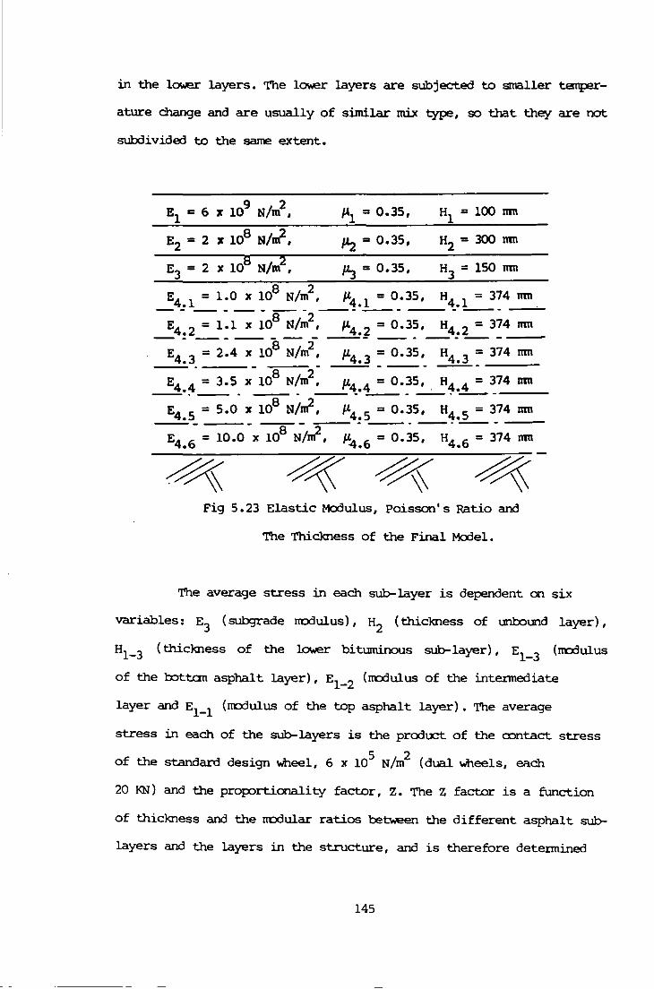
in the lC~o.ei" layers. The la..er layers are subjected to smaller temper-

ature change and are usually of similar m.i.x type, so that they are not

subdivided to the sarre extent.

9 2 E1 = 6 :JC 10 N/rn , f.\ = 0.35, H1 = 100 mn

Fig 5. 23 Elastic Modulus, Poisson' s Ratio and

The Thickness of the Final Model.

The average stress in each sub-layer is dependent on six

variables: E3

( subgrade rrodulus) , H2

(thickness of I.IDl::otmd layer) ,

H1_3 (thickness of the la..er bituminous sub-layer), E1_

3 (II'Cdulus

of the rottan asphalt layer), E1_

2 (rrodulus of the intennediate

layer and E1_1 (II'Cdulus of the top asphalt layer). The average

stress in each of the sub-layers is the product of the cnntact stress

of the standard design wheel, 6 lC 105 N/rn2 (dual wheels, each

20 KN) and the prop.Jrtionali ty factor, Z. The z factor is a function

of thickness and the rrodular ratios between the different asphalt sub-

layers and the layers in the structure, and is therefore detennined

145

for each sub-fayer. For the pavement structure with a granular road

base:

E3

= 10 x 10 7

N/m2 ,

El-l = E1_2 = E1_3 = 6 x 109

N/rn2

,

H2

= 450 mn,

H1_

3 = 20 mn.

The prop::>rtionality factors, z, for this non-typical structure of

100 mn of bituminous material on top of 450 mn of granular material

are not available fran the data tables presented in the Shell Method

(124); tabulated values corresponding to the structure closest to that

investigated were used. Details of these structures and the correspon-

Cling Z factors derived fran the Table Z8 and Table Z48 in the Shell

Manual (124) are given in Table 5. 7 fran which it can bP. deduced that

the Z factors for the 10\\er bi turninous sub-layer lies between 0. 8 and

1.1. This gives an average stress level between 4.8 x 105 and

6.6 x 105

N/m2

in the 10\\er bituminous sub-layer.

Subgrade Thickness of Thickness of the mid Zl Z2 Z3

Modulus,N/m unlx>tmd layer,rnn asphalt sub-layer, rnn

1x108 300 0 -0.3 1.1 -

1x108 300 50 o.o 0.5 0.8

1x108 600 0 -o.l 1.0 -1x108 600 50 0.1 0.5 0.8

Table 5. 7 Prq:ortionality Factor, Z, Derived

fran the Shell Manual (Ref 124).

146

0

1 -

2 -

-

10 20 I

30 I

~ - --- --- - -- -'------....,

- - ------- - ---- - -- - -~------~

---- ---------- --- - -- ----L-------.

5 -

~0 ~0

- - - -- ---- -- . - - - - - - - - - - - -. - --. - - --- --- - '-------- ---------------.

6 -

Fig 5.24 Variation of Subgrade Strength with Depth.

4

8

N I 0 ..-1

X - 16

8 ·.-1

t <1l

..-1

~ 20 ~

28

32

36

Distance Along The Road (m)

4 . 2 4 . 5 5 5 . 5 6 6 . 5 7

... - -- - - - - --- -

-- - - - - -Site

---r-bdel

Fig 5. 25 Canpariscn of Absolute Deflection Along the Line

Through the Centre of the 'IWin Rear Wheels.

148

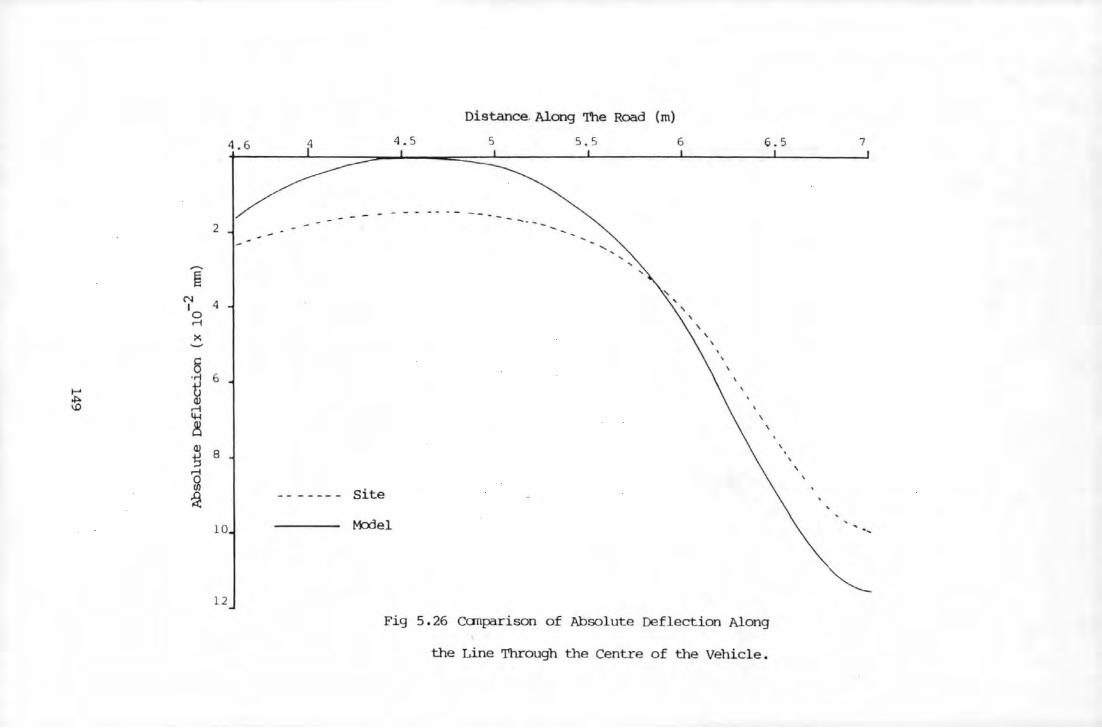
Distance. Along The Road (m}

4 4. 5 5 5 . 5 6 6 . 5 7

- - - - .. - . -2 - -- -

' ,......

s N 4 I

0 ...-4

X ~

8 .£ 6 t-' .p. CV \0 rl

4-l

~ CV

~ 8

g Site ~ - ------

10 t-tdel . ,

12

Fig 5.26 Comparison of Absolute Deflection Along

the Line Through the Centre of the Vehicle.

Distance Along The Road (m)

4

8

-El N I 0

12 r-i

X

8 -~

t 16 (I) r-i 44

8 -a "' f 20

(I) r-i 44

8 24

28

' - ----Site

32 ---t-bdel

Fig 5.27 COmparison of Deflectograph Deflection.

150

The stress at the bot tan of the bituminous layer, on the

vertical axis of syrrmetry between the two loaded areas is greater than

those on the vertical axis through the centre of the loaded area for

the 3D finite element nodel. The stress on the vertical axis of syrnne­

try between the two areas is 1. 7 x 106

N/m2

• This value is slight-

ly greater than that suggested by the charts in the Shell Manual (124)

and it may probably be due to the difference in the magnitude of the

wheel loads, layer noduli and layer thickness. Ho..-.ever, the stress

obtained is not unrealistic, which when taken together with the fact

that the deflected shape of the theoretical nodel was very similar to

that of the actual pavement structure. This suggests that the response

was sufficiently accurate to be used as the basis of an investigation

of the relationship between the deflected surface shape and the prope­

rties and thickness of pavement structures.

5. 6 Fortran Prc?gram to Change Absolute Deflection to De"flectograph

Deflection •

PAFEC program (116, 117, 118) creates an output file, Phase

7, which contains the deflection, in three directions, of all the

nodes in the structures. This output file is quite large and the PAFEC

program does not have the facility to only print the deflection at

certain nodes.

A Fortran Program, called TRANS.F77 (see Appendix IV), has

been written to pick out the vertical deflection, y direction, at

certain particular nodes fran the output file, Phase 7. The nodes

along the centrP. line between the twin rear wheels, line XX of

Fig 5.18, and along the centre line of th~ vehicle (Deflectograph),

line GH of Pig 5.18, have been numbered in an ascending order, i.e. 1

151

to 25. Therefore when the Fortran Program is run, it pidcs up only the

first 25 deflection values in the output file, Phase 7.

Another Fortran Program, _called P'I.J:Jr.F77 (see Append:Uc V),

has been written to mnvert the absolute deflection into Deflectograph

deflection using the following equation (125):

DD= (YBF- Y00 ) - (1/11 ) (YCF- YQ))

- (1 - ~/11 ) (YAF - YN) (5.13)

where yro and YM' = Initial and final deflection of JX>int A;

y00

and YBF = Initial and final deflection of JX>int B;

y00

and Ycr = Initial and final deflection of JX>int C;

12

= Length of T-Datum frame = 2 .13 m;

~ = Length of Measuring Arm = 1 . 53 m.

Ar-------------~c

~========~===========B

A~======I=1====~C Fig 5. 28 Simplified Diagranmatic Representation of Deflectograph.

The program changes all the absolute deflections along the centre line

through the front and twin rear wheels, at either 50, 100, 125, 200 ar

250 mm intervals, into equivalent Deflectograph remrded deflection.

5.7 Sl..lllTIIar)'·

The specification of the final rrodel used to investigate the

relationships between deflected shape and the properties and thickness

of the pavements layers -is sU!l11lai"ised below.

152

(a) LOading.

(i) A square, 170 x 170 mn, contact area was used in the !I'ICX:Iel;

( ii) The loads were applied as pressure loads over the contact

area;

(iii) Only one set of twin rear Wheels, nearside, and front

Wheel were rrodelled;

( iv) Only half of the nearside twin rear Wheels and front Wheels

were rrodelled •

(b) Dimension of r1Qdel.

(i) The distance of the centre of the nearside twin ·rear Wheels

to the kerb is alxmt 1300 mn;

( ii) The dimensions of the rrodel are as follow:

Length = 4500 mn, Width = 2225 mn, Height = 2040 mn (min);

(iii) The rrodel consist of 9 main layers and each layer can be

subdivided into a number of sub-layers. All the main layers

can have different material properties but all the sub­

layers within the main the layer rrrust have the same material

properties;

( i v) The thickness of the main layer and sub-layer within any

main layer must be between 75 to 374 mn.

( c) The Boundary Conditions •

( i) The plane near the kerb is free, i.e. not restr21ined in any

direction;

( ii) The plane through the cut-off plane of the twin rear Wheels

and front Wheel is restrained fran rroving in the x

direction (horizontal longitudinal);

( iii) The plane throu<]h the line along Which the the T-frame rroves

is restrained fran rroving in the z direction (horizontal

153

transverse) ;

(iv) The l01t.er plane of the rrodel is restrained in all directions

Table 5 • 5 shows the restraint applied to the various planes of the

rrodel.

(d) Material Properties.

( i) The material properties required for linear analysis are the

elastic rrodulus, Poisson' s ratio and the density. The

properties required for non-linear analysis are: yield

stress, plastic rrodulus, gradient of the stess-strain curve

before and after yielding and the· size of incremental load.

(e) Element TypeS•

( i) Eight ncxled brick element and sbc noded wedge elements are

used;

(ii) TOtal number of elements used. require~ ~re 2331;

( iii) TOtal number of ncxles required are 2920.

(f) Cmp.~ting Time.

(i) The c::rnp.~ting time required for the analysis of the rrodel

frm the beginning is 24, 600 sec but when the job is

restarte<'l fran phase 6, i.e. when only the material

properties ' of the rrodel is changed, the time required is

only 15,113 sec.

( g) Special Programs.

(i) FOrtran Program, TRANS.F77, picks out the deflection along

the line through the centre of the twin rear wheels and the

centre line of the vehicle,

( ii) FOrtran Program, PI.DI'. F77, =nverts the deflection obtained

frm the rrodel into deflection that would be re=rded by the

Deflectograph.

154

CHAPI'ER 6.0 RELATIONSHIPS BEl'WEEN CURVA'IURE AND/OR DEFLECI'ION AND

THICKNESS AND EI.ASTIC MJOOLUS OF THE VARIOOS lAYERS OF THE PAVEMENI'.

6.1 Introduction.

It would be very beneficial to establish relationships betwe­

·en measurements that can be taken on the road surface and the thick­

ness and elastic m:dulus of the pavement layers, since they could be

used as:

(a) a tool. for identifying the weakest layer( s) of a pavement;

(b) a design t=l to detennine the thickness and elastic m:dulus of

the pavement layers to produce a given surface defle:.ction.

A parametric study has been carried out to develop such rela­

tionships between curvature and/or deflection of a pavement surface

under load and the thickness and the elastic m:dulus of its various

layers. The study involved the use of a 3D finite element m:del of a

pavement in 111/hich the thickness and elastic m:dulus of the various

layers were varied independently. The m:del was used to determine the

distance over 111/hich the surface curvature of the road surface is infl­

uenced significantly by changes in the thickness and elastic m:dulus

of the various layers. Separate routines were developed to convert the

absolute deflected shape predicted by the m:del into the equivalent

deflection dish that would be measured by a Deflectograph. In all

cases the measures of deflected road surface shape or o curvature o ,

used in developing the relationships are those that would be measured

by a Deflectograph.

This chapter attempts to identify same of the factors, i.e.

pavement layer thickness and m:dulus, 111/hich influence the deflection

and the differential deflection recorded by the Deflectograph. The

155

results of the analysis are used in developing an Analytical Pavement

Evaluation and Design system. Various relationships have been establi-

shed between Maximum Deflection, Do• Deflection at distance x away

fran point of maJCirnum deflection, Dx' and Differential Deflections,

D -D (difference in deflection at distances x and y away fran the X y

point of maJCirnum deflection), Equivalent Thickness, He' and the

thickness and elastic ll'Odulus of the various pavement layers.

6.2 Parametric Study.

In a parametric study, the thickness and elastic ll'Odulus of

the various layers of a pavement are changed independent! y, one par am-

eter at a time, and the effects on the resulting deflected shape and

deflection of the pavement under load are obtained. To carry out a

full parametric study covering the range of all variables for every

pavement layer requires a substantial computer resource and, there-

fore, only two different values of elastic ll'Odulus and thickness nor

each layer were considered. Table 6.1 shows the different values of

thickness and elastic ll'Odulus of the different layers. The upper and

lower value of layer thickness and ll'Odulus are considered to represent

the limiting pratical values to be found in l!Dst pavements, see Fig

6.1. Relationships have been established nor different elastic ll'Odulus

and thickness by interp::>lating between the two specified values. Only

linear elastic analysis was carried out. The Defiectograph deflection

derived fran the 3D ll'Odel was used to establish relationships between

maximum deflection/differential deflection of the road surface and the

thickness and ll'Odulus of individual pavement layers.

156

.y

~ ~

~ ~

~ ~ e> ~

e> ~ +

../0..9 lOO 150 J ~ + e- + ../06> ~ ~ + ../0&> 't., ">~ 1 50 300 150 300

../ 0 .> 't., "> ~ ~~ 150 350 150 350 150 350 150 ~ 350

~~

4 2

2 10

9 4

2 10

2 4

9 10

9 4

10

2 4

2 10

9 4

10 10

4 2

9 10

9 4

10

Note: All canbinaticns have been investigated.

Table 6 .1 Different carbinations of the Thickness and Elastic

M:ldulus the Different Layers of Pavement.

157

~

surfacing: Bituminous Naterial:

El = 4 - 10 X 109

N/rrf: H1 = lOO - 150 mn. H 1 ~

• Road Base: Granular Material:

E2 = 2 - 9 X 108

N/m2

: H2

= 150 - 300 mn. H2

~ 1\; Hp-

Sub-base: Granular Material:

8 2 E3 = 2 - 9 x 10 N/m : H3 = 150 - 350 mn. H3

'

Subgrade: CBR 2 - CBR 10:

7 2 E4 = 2 - 10 X 10 N/m •

Fig 6.1 Range of Thickness and Elastic Modulus of Individual Pavement

Layers.

6.3 Selecting the Position of a Suitable Ordinate Differential

Deflection •

The results of the parametric Study shcJI...ecl that the shape in

the vicinity of the maximun deflection can be used as an indicator of

the strength of the upper l::ound layer. The next step was to select the

position of the ordinate deflection within this area whose changes in

magnitude, as a result of changes in the thickness and modulus of the

layer, was large enough to be recorded by a Deflectograph. Deflection

parameter, Dx' decribed in this thesis refers to the vertical surf-

ace deflection of the pavement at distance x away fran the point of

maximum deflection. Differential deflections, Dx -Dy, refers to the

difference in the vertical surface deflection of the pavement at dist-

ances x and y away fran the point of maximum deflection.

158

The suitable p::>sition and distance over which the different­

ial deflection (recorded by Deflectograph) should 't;le obtained is dete­

rmined by o:mparing the magnitude of the differential deflections over

various distances throughout the deflected dish. The p::>sition of the

differential deflection, used to characterise a particular parameter,

was selected as the p::>int at which the maximum change in differential

deflection is produced for a small change in the parameter considered.

Fig 6. 2 shows the deflected shape recorded by the Deflectograph and

the symbol used to represent the deflection ordinates at various dist­

ances away fran the p::>int of maximum deflection. Fig 6. 3 illustrates

the method used to obtain the ITDSt suitable p::>sition and the distance

at which the differential deflection should be measured. The example

presented in Fig 6.3 relates the differential deflections D0-DB to

the equivalent thicknesses, He' for a given value of ft• see Fig

6.7. Fran the graph it can be seen that the maximum differential

deflection is D0-DB (i.e. difference in deflection at p::>int 0 mm

and BOO mm away fran the p::>int of maximum deflection).

This procedure was adopted to obtain the ITDSt suitable p::>sit­

ion and distance of the differential deflection for the change in the

thickness and elastic modulus of the various layers.

6.4 Method of Statistical Analysis.

In order to develop an analytical pavement evaluation and

design system, relationships must be established between the Deflect­

ograph deflection/differential deflection and the thickness and

modulus of individual layers of the pavement. Several relationships

were investigated but in many casses the variation of the original

data demonstrates that estimates of predicted layer properties could

159

not be made with reasonable levels of statistical confidence.

6.4.1 Regression and Fitting of COmmon Slope.

The statistical analysis was carried out using canp..~ter based

Statistical Analysis packages. called MINITAB (126) and GLIM (127).

Several statistical .rrcx:lels, i.e. Pol.o.er, E:>q:onential and Polynanial (k

orders), ....ere fitted to investigate the relation between the differen­

tial deflection and pavanent layers thickness and rrcx:lulus. The R-Squa­

red, i.e. (Sum of squares explained by the regression/Sum of squares

of the independent variables), were canpared for all the statistical

rrcx:lels and the rrcx:lel which gave the largest value of R-squared was

identified. The Power Law rrcx:lel gave the largest value R-squared and

was linearised by plotting r.og10

Y Vs r..og10

x. When investigating

the difference in several regression lines for the different pavement

layer variables, i.e. rrcx:lulus and thickness, the follO'Wing procedures

....ere carried using the Statistical Package GLIM (127):

(a) Fit separate lines, linearised by plotting r.og10Y Vs r.og10x,

(different slopes and intercepts).

(b) use the F-test in the analysis of variance to test for significant

difference in slopes. If the differences are not sig.nificant then

a mlDlou slope (different intercepts) can be fitted for the

different lines.

(c) Once parallel lines have been established, they are then tested

for a mmon line, i.e. single intercept. The analysis of variance

is carried out using F-test to test if there is any significant

difference in intercepts. If the differences are significant then

the lines remain different and only a · mtUIOII slope is fitted.

Details of the statistical analysis are shown in Appendix VI.

160

-e N I 0 12 ...... X -8 ..... ti HI Q)

...... 1+-4

~ t 10

f 20

...... 1+-4

~ 24

21

32

Distance Along The Road (m)

6.4 8.6 CS. 7 CS. 8 4.8

D 6

'b- o •

----------- ----

o,

Fig 6. 2 Nanenclature to Represent the Deflection

Ordinates at various Distances Away fran

the Point of Ma.XimLJTI Deflection.

161

D 0

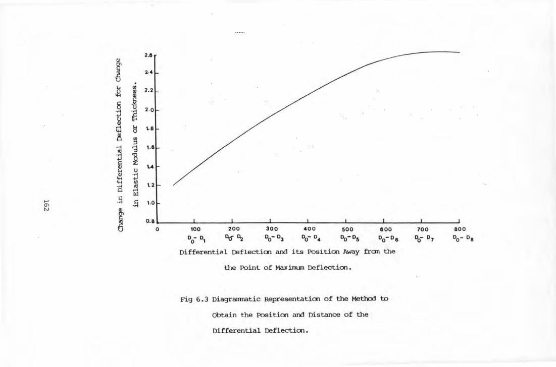
<1.1

! ~

~

8 -~ ..... ~

~ ..... 10 •j c: ~ <1.1 ~ ~ ·ri Cl

t-' .s 0'1 N <1.1

!

. IJ) 1.0 <1.1

~ ~ ~ 1.0 :J

3 ~ u •j 1.0 10 ..... ~

.s

2..0

1.8

0.8~-------L--------L--------L--------~------~--------L-------~--------l 0 100

D-D 0 1

200

000-z

Differenti<'l Deflecticn and its PositiCt'l PMay fran the

the Point of Maximun Deflecticn.

Fig 6. 3 Diagrarnnatic Representaticn of the Metb:rl to

Obtain the Posi tiCt'l and Distance of the

Differential Deflecticn.

6.4.2 COnfidence Limit.

The 90% a:mfidence limits for a future predicted observation

have also been calculated using the t-test for the relationships

defined in Section 6.4.1 arove. The confidence limits are the band

width within which 90% of the results of the different types of struc­

ture a:msidered fall, i.e scatter of data. The band represent the

rqnge of data fran the weakest structure, i.e. canbination of all the

minilnum thicknesses and rroduli of each layer, to the strongest struct­

ure, i.e. canbination of all the maximum thicknesses and rroduli of

each layer. It is also the band width within which 90% of the future

predicted analysis will fall. 90% of the pavanents with structure

within the range specified in Fig 6.1 will fall within this band.

Pavanent structure for rrotorways and other rrodern designed roads might

be expected to have sanewhat narrc:J~.o.er 90% confidence limits if good

quality control has been achieved in layer properties and thickness.

An example of the regression line and the 90% confidence limits are

shown in Figs 6.4 and 6.6.

6. 5 Relationships Between Deflected Shape and Pavanent Condition.

6. 5 .1 Relationship between o8 and CBR of Subgrade.

Several authors, using various measuring equipment (15, 31,

32) , have reported that the deflection at sane distance away fran the

point of maximum deflection is a measure of support strength. The

distance fran the point of maximum deflection at which the deflection

is taken depends on the types of equipnent used. It seems that for the

Deflectograph, the deflection at a distance 800 rnn away fran the point

of maximum deflection is a good indicator of the support strength.

163

Analysis of the effect of different CBR of the subgrade on

the response of the finite element rrodel has led- to the derivation of

a relationship between the deflection at distance BOO mm away from the

~int of maximum deflection, o8 , and the CBR of the subgrade. Varia­

tion of elastic rrodulus and thickness of each layer al::ove the subgrade

for a given CBR has only a very' small influence on the o8 •

Fig 6.4 shows the ~Law relationship between o8 and CBR

with 90% confidence limits. Table 6.2 shOW'S the equation todescribe

the relationship. From this relationship, it is ~ssible to detennine

the CBR of the subgrade knowing the deflection, o8 • For a given o8

of 0.004 mm the relationship predicts a CBR of 2% with a 90% confiden­

ce limits of :::=1% (see Fig 6.4}. It predicts a CBR of 7% with a 90%

confidence limits of :::= 2% for a given o8 of 0.002 mm. The confidence

limits band narrows at higher CBR since the variation in o8 reduces

as the subgrade increases in strength when other pavement variables,

i.e. layer thickness and rrodulus, have negligible influence on o8 •

TO predict the subgrade strength requires that the Deflectograph can

measure to 1 p.m.

Equations No

UlglO(DB) = 0.776- 0.572 UlglO(CBR} 6.1

Table 6.2 Equations to Describe The Relationship Between o8 and CBR.

164

•

e 90% Ccrlfidence Limit

-E 3 • E N I 0 ~

X -CO

~ 0 0\

2 V1

•

CBR

Fig 6.4 Po.-.er Law Relaticnship Bet:v.een o8

and CBR.

6.5.2 Relationships Between Maximum Deflection, D0 , and Equivalent

Thickness, He·

Equivalent Thickness, He' for a four layer system is defin-

ed as follows (80, 81, 82):

He = 0. 8 lC ( H~ + ~ + H~ ) 3-(6.2)

E4 E4 E4

where He = Equivalent Thickness;

Hl = Thickness of Surfacing;

H2 = Thickness of Road Base;

H3

= Thickness· of Sub-Base;

El' l-'1 = Elastic Modulus and Poisson's ratio of Surfacing;

E2' 1-'2 = Elastic Modulus and Poisson' s ratio of Road Base;

E3' 1'-3 = Elastic Modulus and Poisson' s ratio of Sub-Base;

E4' /J.4 = Elastic Modulus and Poisson's ratio of Subgrade.

This equation (Eqn.6.2) allows a four layer system to be transferred

into a one layer system of thickness, He. In the parametric study,

the Poisson's ratio for all the layers was assumed to be 0.35.

The maximum deflection, D0

, was plotted against He for

various CCITlbinations of pavement structures investigated, see Table

6.1, on t...o different subgrades: CBR 2 and CBR 10. Fig 6. 5 sho.vs the

scatter of the data for CBR 2 when the Log10 (D0 ) is plotted again­

st Log10 (He). The Power Law equations to describe the relation

ships are shown in Table 6.3. A ccmron slope could not be fitted for

the two CBR levels using the procedures stated in Section 6.4.1. Fig

6.6 illustrates the relationship with the 90% confidence lirnQts. It

seems that the max:iJnum deflection, D0

, is greatly influenced by He.

The linesof the t...o CBRs tend . to converge at a higher value of He or

at lo....er value of max:iJnum deflection, i.e. when the pavement is very

166

stiff. For the various a:rnbinations of structures investigated, the

range of He for CBR 2 is 0.98 to 2.8 m and for CBR 10 is 0.58 to

1.64 m. The minimum and ma.J(:i.rnum value of the He range represents the

weakest and strongest structure of the a:rnbinationsof structures inve­

stigated. At the 90% confidence level, the relationship for CBR 2

predicts a value of He: 1.5 := 0.2 m for D0

of 0.27 mn. To give

sane engineering appreciation of this variation, a confidence interval

of He: := 0. 2 m about the mean value .....ould result in the following

variations in the thickness and rn:x:lulus of pavement layers when conve­

rted back into individual properties:

E1 = Variation of:= 4.0 E1 (mean);

E2 = E3 =Variation of :=4.0E2 (mean);

H1 = Var.· iation of := 1.5H1 (mean);

H2 = H3 = Variation of := 1.4H2 (mean) •

For CBR 10, a D0 of 0.2 nrn gives a 90% confidence range of He:

0.82 :!: 0.16 m. This confidence interval of He: :!: 0.16 m about the

mean value has the sarre order of variation in the pavement variables

as CBR 2. A small variation of He .....ould change any '"? rn:x:luli .. -of the

pavement layers, i.e. E1 , E2 , E3 , by 2 to 3 t..ilres. He is

influenced rrore by the rn:x:lulus than the thickness of the pavement

layers. This shows that the rn:x:lulus of the pavement layers should not

be cletermined fran any relationship having He as one of the variab­

les.

CBR Equations No

10 LoglODO = 1.197 - 1.23 LoglOHe 6.3

2 Log10°0 = 1.731 - 1 . 73 LoglOHe 6.4

Table 6.3 Equations for the Relationships-Between o0

and He.

167

40

+

+ + 30

+

- + + E + + + E +++ * +

N + + ++ I 0 20 ~ +

X + + + ++ - + +*

0 0

+ -1- 1-

++ +

+ ++ +

+ ++

++ + +

+ ++

10 + +

9 + + +

8 +

5L-----~~----~--~~--~--~~~--------------------~ ·4 . 5 • 6 • 7 • 8 • 9 , 2

He(m)

168

•

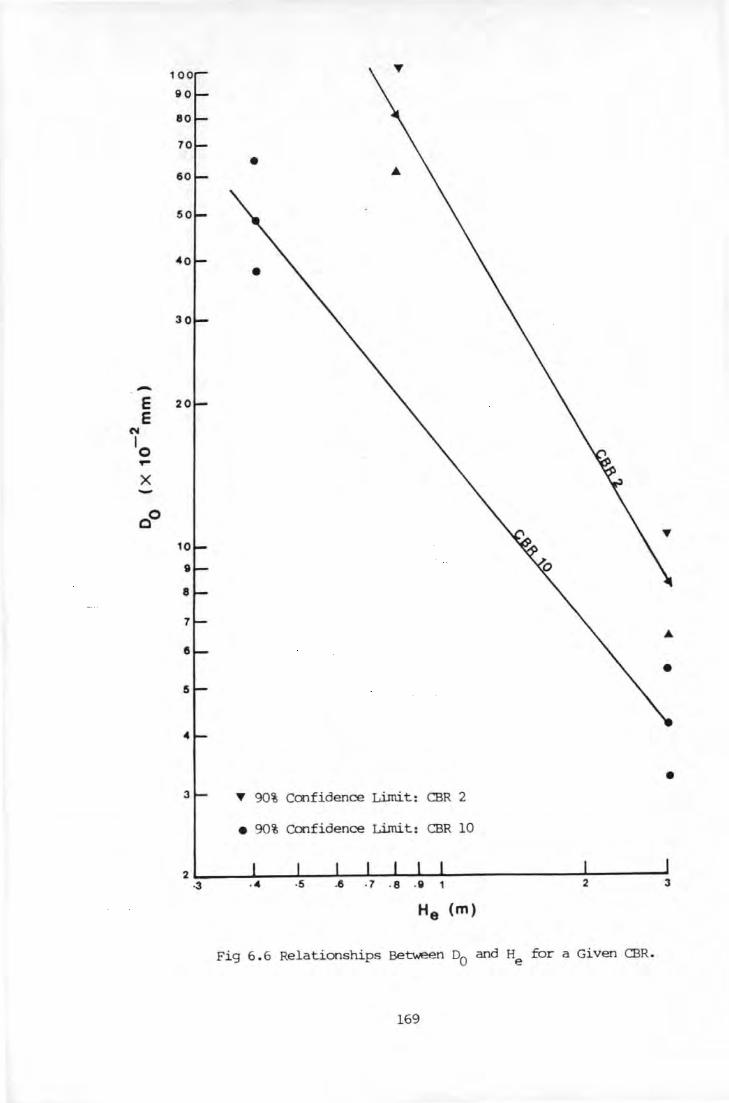
-E 20

E N

10 ~

X -00

• ~ 90% Confidence Limit: CBR 2

• 90% Confidence Limit: CBR 10

. 7 .s .e 2 3

He (m)

Fig 6.6 Relationships Between n0 and He for a Given CBR.

169

6.5.3 Relationships Between o0-o8 and He fOr a Given Thickness

of Granular Material, ft; (H2+H3 ) •

In ITOst pavanents, containing a granular road base, the road

base and the sub-base are constructed with similar material, i.e.

having a similar ITOdulus value when canprred with the ITOdulus of lay­

ers inmediately above and below. Relationships between differential

deflection and equivalent thickness fOr a given value of road base,

H2

, and sub-base, H3, have been investigated but no practical

relationships that could be used to interpret site measuranents were

established. TherefOre, H2 and H3 were a:rnbined together as. ft;

(total thickness of granular material) and relationships were establi­

shed between He and differential deflection, o0-o8 , for a given

value of It· The differential deflection, o0-o8 , was plotted against

He' fOr a given thickness of granular material, It (H 2+H3 ),

see Fig 6.1. A camon slope was fitted fOr the different regression

lines. The statistical details and the Pov.er Law equations to repre­

sent the relationships are shown in Tables A.l and A.2 of Appendix VI.

The variation of the thickness of granular material greatly influences

the differential deflection, o0-o8 • It is possible to determine

It fran Fig 6.7; knowing He (see Fig 6.6) and CBR (see Fig 6.4).

The following information could be deduced fran the relationships:

Given: CBR 2: It = 300 mm: o0-o8 = 0.3 mm:

Prediction: He= 1.21 ::!:: 0.1 m at 90% confidence limits;

Variation in the thickness and ITOdulus of pavement layers due to the

confidence interval of He =::!:: 0.1 m:

E1: ::!:: 1.6E1 (mean):

H1 : ::!:: 1.2Hl (mean):

170

This clearly indicates that by knowing % and CBR, the variation of

E1

due to variation of He' or vice-versa, is small. The variation

for CBR 10 is of same order as for CBR 2.

6.5.4 Relationships Between D0-D8 and He fOr a Given Pavement

Thickness, Hp (H1+f\/· The differential deflection, D0-D8 , was plotted against

He' for a given pavement thickness, Hp (H1~), see Fig 6.1.

Table A. 3 of Appendix VI shows the equations describing the relation-

ships.

It is observed that the differential deflection, D0

-D8 ,

is influenced by the variation of the total pavanent thickness, Hp·

The relationships could be used to determine Hp from Fig 6.8; know­

ing He (see Fig 6. 6) and CBR (see Fig 6. 4) • The following informat­

ion could be deduced from the relationships:

Given: CBR 2; H = 400 mn· p '

Prediction: He = l. 2 ::!: 0 .1 m at 90% confidence limits;

Variation in the thickness and modulus of pavanent layers due to the

confidence interval of He = ::!: 0 .1 m:

El: ::!: l. 7E1

(mean); ~: ::!: l.4EG (mean);

Hl: ::!: l. 2H1

(mean); It= ::!: l. 2f\; (mean);

Given: CBR 10; Hp = 600 mn; D0-D8 = 0.3 mn;

Prediction: He = o. 75::!: 0.05 m at 90% confidence limits;

The variation in the thickness and modulus of pavanent layers due to

the confidence interval of He = ::!: 0. 05 m is of the same order as for

CBR 2 detailed arove. The value of H1

(thickness of surfacing) could

be determined by subtracting f-b from ~ for a given CBR, He and

Da-Ds·

171

-E E

~ 0 ... X -of!IJ I 00

2 0

CBR 2

• 90% Confidence Limit:Hc;: 300 nrn

o 90% Confidence Limit:Hc;: 500 nrn

CBR 10

T 90% Confidence Limit:Hc;: 300 nrn

v 90% Confidence Limit:~:SOO nrn

CBR 10 &

CBR 2

Fig 6.7 Relationships Bet......een D0

-D8

and He for a Given~·

172

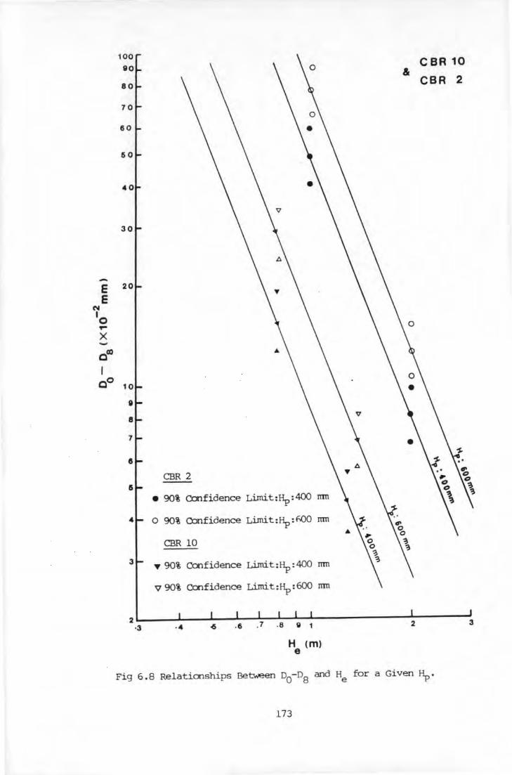
-E E

N

10 ,.. X

ctiJ I CO

20

CBR2

• 90% CCrlfidence Li.mi t: Hp: 400 mn

0 90% Confidence Li.mit:Rp:hOO mn

CBR 10

~ 90% Confidence Li.mi t: Hp: 400 mn

v 90% CCrlfidence Li.mit:Rp:600 mn

H (m) e

& CBR 10

CBR 2

Fig 6.8 Relationships Between o0-o8 and He £or a Given Hp ·

173

6.5.5 Relationships Between o0-o8 and He for a Given Value

E1/E2 Ratio.

Relationships between o0-o8 and He for a given value of

E1/E2 (surfacing modulus/road base modulus) ratio and E2 have

been established. It is observed that the variation of E/E2 ratio

largely influences the differential deflection, o0-o8 • The Power

Law equations for the relationships are shown in Table A.4 of Appendix

VI. The regression lines, see Figs 6.9, 6.10, 6.11 and 6.12, for the

different E/E2 ratios tend.·· to converge at high values of He'

i.e. thicker and/or greater modulus of one or !!Ore layers of the pave-

mer)t. To use the relationships; He' o0-o8 , and E2 have to be

known. The relationships could be interpreted as folla.vs:

Given: CBR 2; o0-o8 = 0.1 rrm;

E/E2 = 40/2.

Prediction: He= 1.6:::!::: 0.3 m at 90% confidence limits.

The variations in the thickness and modulus of the pavement layers due

the confidence interval :::!::: 0. 3 m are as folla.vs:

It: :::!::: 1.4It (mean) •

Given: CBR 10; 8 2 E2 = 2 x 10 N/m ;

E/~ = 40/2.

Prediction: He = 0. 76 :::!::: 0.4 m 90% confidence limits.

Variations due to the confidence interval He = :::!::: 0. 3 m:

It: :::!::: l.Bf\; (mean) •

For the calculation of variation in H1 and It• the values of E1

and E2 were kept constant since the ratio is known.

Fran the relationships it is possible to determine E1 know­

ing E2 • In !lOst pavements with a granular road base, the sub-base

and road base are of similar material, i.e. having similar modulus

174

values when compared with the nodulus of layers imnediately above and

below. Therefore, E2 may be obtained fran tile following equation

(73, 74):

E2 = E3 = K E4

where K = 0.2 s3°• 45; 2<k<4;

E3

= SUb-base Modulus;

(6 .5)

H3

= SUb-base Thickness;

E4 = Subgrade Modulus.

Once E2 is known, E1 ll'BY be determined fran tile relationships.

6.5.6 Relationships Between o0-o2 and H1 ~r a Given Ratio of

E/E2 •

Relationships have been derived between o0-o2 and s1

~r a given value of E/E2 ratio and E2 • Table A.6 of Appendix

VI show tile equations to describe tile relationships. The relationships

are independent of tile support strength, i.e. CBR. The value of s 1

may either be obtained fran subtracting It, fran f1, or by coring

fran tile pavement. The relationships may be used to determine either

tile value of H1 knowing tile ratio E/E2 or tile ratio E/E2

knowing H1 • It could be observed fran Figs 6.13 and 6 .14 that tile

slopes of the regression lines are gentle, i.e. tile rate of change of

o0-o2 with H1 is very low. For a given o0-o2 of 0.07 mm and

E/E2 ratio of 400/20, the relationship predicts a range of s1 =

120 :!:: 20 mm. The confidence interval for other ratios of E/E2 is

about :!:: 25 mm. This sho.Ys that the relationships could predict H1

to a nearest value of 50 mm. The confidence interval width narrows for

tile regression lines as s1

increases.

175

,.. E E

N I 0 ,.. I( .....

•

20

CBR 2 8 e2 =2')(.10 N/m2

• 90% Confidence Limit:E/E2

: 40/2

'Y 90% Confidence Limit:E/E2: 100/2

He <m> Fig 6.9 Relationships Between o0-o

8 and

s I 2 E1/E2 and E2 = 2 x 10 N m •

176

H for CBR 2 for Given e

"" E E

N I 0 -)( ...., QttJ

CBR 2 8 2

~=9X10 N/m

20 •

• 90% Ccnfidence Limit:E/E2 : 40/9

• 90% Confidence Limit:E1/E2 : 100/9

2~----------._--~ __ ._ ____ ~~--------------_. ________ __ -3 "" •5 ft/~: )( 108 N;m2

2 3

H8

(m)

Fig 6 .10 Relationships Between D0 -D8 and He for CBR 2 for Given

8 2 E

1/E2 and E2 = 9 x 10 N/m •

177

e "'

e I 0 ... X ~ttJ

eo

20

10

8

7

•

CBR 10 8 2 e2 = 2 X10 N/m

• 90% Confidence Limit: E1/E2 = 40/2

~ 90% Confidence Limit: E1/ E2 = 100/2

.3 .4 .5 .e . 1 .a . e 1

E1/E2 : M 108 N/m2 H

8(m)

Fig 6.11 Re1ati~ships Between D0-D8 and H for CBR 10 for Given e 8 2

E/E2 and E2 = 2 x 10 N/m •

178

,... e

"e I c ... • ...., c= I CO

• 20

• 10

• a

7

&

5 -4

3 • 90% Confidence Limit:E1/E2: 40/9

~ 90% Confidence Limit:E1/E2: 100/9

· e ·7 ·e ·Q 1

CBR 10 8 2

~=9X10 N/m

2 3

Fig 6.12 Relationships Between D0-D8 and He for CBR 10 for Given

8 2 E1/E

2 and E2 = 9 x 10 N/m •

179

-E E

C"-1 I 0 ~

X -QN

I oo

20

10

4

3

2

'f'

b. £r Y~:::::. 1o0 <%

<o

'f' 90% Confidence Limit:E/E2 : 40/2

v 90% CCnfidence Limit:E/E2: 100/2

b.

1~~------------------------------------------~--100 150

Fig 6 . 13 Relationships Between o0-o

2 and H1 for Given

Ratio of E/E2 and E2

= 2 x 108 N/m2 .

180

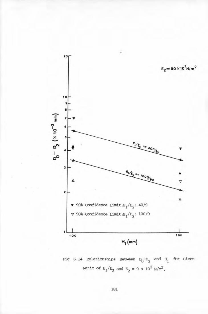
-E E

('ill

I 0 ... X ._ Q~

I eo

20

4

3

"' 90% Ccnfidence L.imi t: E/E2: 40/9

v 90% Confidence Limit:E1/E

2: 100/9

1~~------------------------------------------~--100 1 50

~(mm)

Fig 6 . 14 Relationships BebNeen o0-o

2 and H

1 for Given

Ratio of E/E2 and E2

= 9 x lOB N/~.

181

6.5.7 Relationships Between o0-o2 and E1 £Or a Given Value of

E2 and H1 •

Power Law relationships have been established between differ-

ential deflection, o0-o2 and E1 £Or a given value of E2 and

H1 • The equations to represent the relationships are given in Table

A. 7 of Appendix VI. It is observed that the differential deflection,

o0-o2 , is greatly influenced by the variation of E1 £Or a given

value of E2 and H1 • The regression lines tend, see Figs 6.15 and

6.16, to converge at higher values of E1• This indicates that as

El increases, the pavenent becanes stiff and o0-o2 is incapable

of detecting the different values of E2

• By camparing the regression

lines for H1 of 100 and 150 rrm for a given E2 , it could be seen

that the regression line for H1 : 150 rrm would intercept the x axis

at lower value of E1

than the regression line H1

: 100 rrm.

Given o0-o2

= 0.07 rrm, E2

= 20 x 107 N/m2 and H

1

= 100 rrm, the relationship predicts 90% confidence limits of E1 =

-+- 1. 25E1 (mean E1 = 6. 5 x 109 N/m2 ) • The confidence interval

is of same order, i.e.:::!: 1.25E1 (mean), £Or H1 = 150 rrm and E2=

20 x 10 7

N/m2 • The value of H

1 could be obtained by subtracting

1-b fran Hp or by coring fran the pavenents. The value of E2

could be obtained fran the relationships established in the last few

sections or fran Eqn.6.5

182

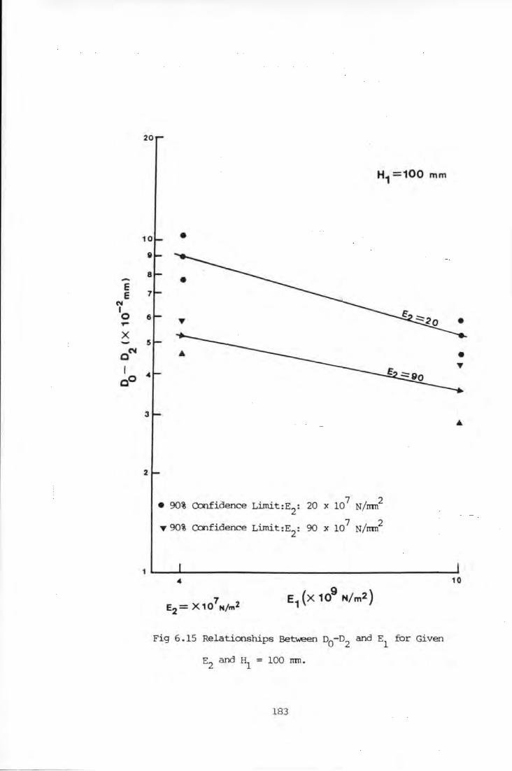
.... E E

N I 0 ~

X

0('4

I ao

20

3

2

H1 =100 mm

•

e 90% Ccx1fidence Limit:E2

: 20 x 107

N/nm2

~ 90% Confidence Limit:E2

: 90 x 107 N/nm2

Fig 6.15 Relationships Between o0-o

2 and E

1 for Given

E2

and H1

= lOO mm.

183

10

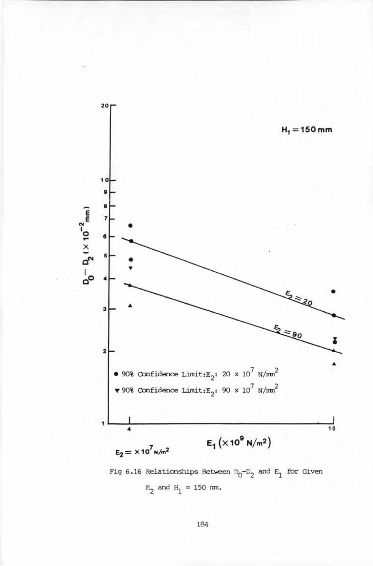
E E

N

10 ~

X

QN

I CO

20

e

2

•

e 90% OJnfidence Lirnit:E2: 20 x 107

N/nm2

~ 90% Ccnfidence Lirnit:E2

t 90 x 107

N/nm2

H1 =150mm

1 ~--~------------------------------------------~

7 ~=X 10 H/m2

Fig 6.16 Relationships Between o0-o2 and El nor Given

E2 and H1 = 150 rnn.

184

10

6.6 Analytical Pavement Evaluation and Design System.

AA analytical Pavement and EValuation and Design System flov.r

chart, Fig 6 .1 7 , has been drawn up based on the relationships establi-

shed in the previous section. The Deflectograph deflection measurem-

ents required for input to the system are D0

, D2

and D8

• The

Deflectograph deflections should be adjusted to equivalent values at

the standard temperature of 20 °c using the appropriate temprrature

correction charts in LR 833 (12). The differential deflection between

t1NO points should be calculated first fran the recorded Deflectograph

0 deflection and then adjusted to equivalent values a 20 c.

Differential deflections are used in the relationships to

obtain the rn::xJulus of E1 or the rn::xJular ratio E/E2 • The deflec-

ted shape recorded by the Deflectograph is influenced by the thickness

and rn::xJulus of the pavement layers at the temperature at which measur-

errent are obtained. The rnaJCimum deflection is influenced primarily by

the rn::xJulus of pavement layers. In order to derive appropriate rn::xJuli

values, therefore, it has been found necessary to use as measured

differential deflection and correct these to the standard temperature

to give the appropriate values of rn::xJuli. Leger et al (23) reported

that the curvature (similar to differential deflection) need not be

corrected for temprrature if it is within the limits specified in

Ref (23).

6. 7 Limiting Factors.

The investigation of relationships developed shov.rs that it is

not possible to determine H2 and H3 separately and and

H3 have to be ccmbined together as ft. H1 can not l::e determined

independently of other pavement variables. Therefore H1

can only l::e

185

determined fran Hp-f\; or fran relationships which involve knowing

E/E2 ratio and E2 • It is not possible to detennine E1, E2

and E3

separately and independently of other pavement variables.

Only the rrodular ratio E/E2 <Duld be detennined fran the relati­

onships established. E1 <Duld be determined fran Figs 6.15 and 6 .16

if H1

and E2

is known. Fran the investigations, it is observed

that E2 (= E3 ) have to be known first before any of the relation­

ships could be used. E2 or E3

<Duld be determined fran Eqn.6.5

knowing CBR of the support fran Fig 6. 4. To avoid build up of errors,

i.e. errors in ~ and !\;, it is better to determine H1 by

coring fran the pavenent.

6.7.1 Insignificant Relationships.

Several relationships have been rejected on the grounds that

the confidence limits for the variables considered, overlap· An exam­

ple of this is shown in Fig 6.18 for the relationships between differ­

ential deflection o0-o3

and equivalent thickness, He' for a

given thickness of surfacing, H1 . For a given He of 1 m and

o0-o3 of 0.1 mm, the relationship could predict an average value

of either 100 or 150 mn. The relationship is not therefore an accurate

indicator of H1 and so it is rejected.

186

~

I

f. Cl

1 ) INPUT

Do, 02, Ds

l 2) CBR --Fig 6 . 4

~ 4) :J:

--+ F i g 6.8

1---+ 5) HG --

1---+ Fig 6.7

,/ 6) Hl -

- :- Hp -HG or Coring

7) E2 -

Eqn 6.5

8) El / E2 ~

...._ __...

Fig 6.9 - 6.12

en 1.0 r1"

~ 0.. Ill CO .j.) en

~

(continued overleaf)

3) He --Fig 6 . 6

~ -

en r1" CD '0

" ~

0 0

I

0 I\.)

Step 1

Requir ed Deflectograph deflection o0 , o2 , o8

Step 2

Knowing o8 determine CBR .

Ste p 3

Knowing CBR & Do, determine H·e

Step 4

Knowing CBR, He & Do - o8 , d e termine Hp

_Step_2

Knowing CBR, He & Do - o8 , determine HG

Step 6

Knowing Hp a nd ~' determine H1

Step 7

Knowing fiG and CBR, determine E2

Step 8

Knowing He, CBR , E2 and Do - os, determine

o E1/ E2 p I

0 I\.) ,

Fig 6 . 17 Flow Chart: Analytical Pavanent Evaluation and Design System.

187

(continued)

9) H1 -Fig 6.13

10) E1 /E2 ---.. Fig 6.13 - 6.14

11) El -Knowing E1 / E2 & ~2

----- -----12)

Knowing E1 / E2 & E2

---- ----13)

Fig 6.15 & 6.16

Ul Ul rt rt m m 'tl '0

CD -...J

"" ....

~

~ I

~

0 0

I

0 N

Step 9

Knowing E1/E2 (Step 8) & Do - D2, determine H1.

Step 10

Knowing H1 , E2 & Do - D2, determine

E1 / E2

Step 11

Knowing E1/E2 (Step 8) & E2, determine E1.

Step 12

Knowing E1/ E2 (Step 10) & E2, determine El.

Step 13

Knowing H1 , E2 and

Do - D2, determine E1

Fig 6.17 Fl()IN Chart: Analytical Pavement Evaluation and Cesign System

( rontinued) •

188

-E 20 E N I 0 ,.. X -CM

I eo

•

•

•

• +

+

•

+

• 90% Ccnfidence Li.m:it:H1: lOO mn

+ 90% Ccnfidence Li.m:it:H1: 150 mn

H8

<m>

CBR 2

•

+

•

+

Fig 6.18 Relationships Between o0-o3 and He for CBR 2 for

Given H1 •

189

6.8 Surrmary.

(a) Relationships Between Deflection and/or Differential Deflection

and Layer Thickness and Modulus.

( i) CBR (E4

) mainly influences D8

;

(ii) E1/E2 ratio mainly influences D0-D8 ;

(iii) El llBinly influences D0-D2 for a given H1 and E2•

(iv) Hl llBinly influences Do-D3;

(v) Hl l!Binly influences D0-D2 for a given value of

E/E2 and E2 •

(vi) He; rrainly influences Do-D8;

(vi) Hp rrainly influences Do-D8:

(vii) He mainly influences Do:

(b) Required Deflection Inputs •

In order to use the relationships, the following ordinate

Deflectograph deflections are required:

(c) SupfC>rt Modulus, CBR.

The CBR of the support can be detennined fran the deflection,

D8 , see Fig 6.4.

(d) Equivalent Thickness, H • e

He= (0.8 x Hl h 1/E4 ) + (0.8 x H2 h/E4 )

+ (0.8 x H3 ~E3(E4 ) (6. 2)

The equivalent thickness, He' may be obtained fran the relationships

betlil/een maximum deflection, D0 , and He' see Fig 6.6.

190

(e) Thickness of Surfacing, H1 •

Relationships betw-een the differential deflection, o0-o2

and He may be used to determine H1 for a given value of E/E2

and E2, see Figs 6.13 and 6.14. H1 may also be obtained by subtr­

acting 1'\; (Fig 6 • 7 ) fran f1, (Fig 6 • 8 ) • Hov.ever, to prevent a build

up of errors, H1

should be determined by coring.

(f) Thickness of Granular Material, ft.

In rrost pavements, with a granular road base, the road base

and the sub-base are constructed with the similar material, i.e. hav­

ing a similar rrodulus- value when ccmpared with the rrodulus of layers

irrmediately above and below. Therefore, the total thickness of granu­

lar material, ft, is determined fran the relationships between the

differential deflection, o0-o8 and equivalent thickness, He' see

Fig 6.7.

(g) Total Thickness of the Pavement Layers, ~·

Relationships between the differential deflection, o0-o8

and equivalent thickness, He, may be used to determine the total

thickness of the pavement, i.e H1 + ft• see Fig 6.8.

(h) Elastic Modulus of Surfacing, E1

.

Relationships betw-een the differential deflection, o0-o8 ,

and He may be used to determine the values of E1

, if E2 is

known, see Figs 6.9, 6.10, 6.11 and 6.12. Relationships between

o0-o2 and H1 may also be used to determine E1 if H1 and E2

are known.

191

( i) Elastic Moclulus of Road Base, E2

or Sub-Base E3

•

The similarity of material in rrost granular road base pave­

ments results in ccrnparable values of E2 and E3 nodulus, and

therefore it may be obtained fran the relationships between o0-o8

and He if E1 is known, see Figs 6.9, 6.10, 6.11 and 6.12. It may

also be determined fran Figs 6.13, 6.14, 6.15 and 6.16 if H1 and

E1

are known. Alternatively E2 = E3

may be calculated fran

Eqn.6.5.

( j) Analytical Pavement Evaluation and Design System.

Based on the established relationships, an Analytical Pavem­

ent Evaluation and Design System flow chart has been drawn up, see Fig

6.17. Validation of the system and the effects of errors (confidence

interval) on the predicted values fran the system are discussed in

Chapter 7 • 0.

192

rnAPI'ER 7.0 VALIDATION OF THE ANALYTICAL PAVEMENT EVAil.JATION

AND DESIGN SYSTEM.

7 .1 Intrc:duction •

An Analytical Pavement EValuation and ~sign System has been

set up in Chapter 6.0. The design system was calibrated using deflect­

ion results obtained fron the TRRL. To validate this system, requires

Deflectograph deflection measurements together with information about

the thickness and nodulus of the layers of the pavement with which to

cx:mpare predicted values of the layers' properties. The ~flectograph

deflection used as input was obtained fran the ~flectograph surveys

conducted previously on local roads (131). Cores of bituminous ll'ater­

ial were extracted fran these roads to detennine the thickness, and

laboratory triaxial testing was undertaken to determine the nodulus of

these layers. In-situ bearing capacity tests using a cone penetraneter

were carried out previously by Bu.tler: (131) on these roads to determ­

ine the subgrades type and strength. Information about the road base

construction was also obtained fran the previous work ( 131) •

Using the in-situ ~flectograph deflection (131) as an input

the thickness and elastic nodulus of pavement layers have been predic­

ted using the Analytical Pavement EValuation and ~sign System set up

in Chapter 6.0. The predicted layer's thickness and nodulus have been compared

with those occurring in the real paveilent structure.

193

7. 2 Thickness and Modulus of Pavanent Layers.

7.2.1 Bituminous Material.

The lal::oratory triaxial testing of the bituminous material is

described in Appendix VII. The elastic l!Ddulus of the bitlUllinous

samples was between 2 • 5 to 5 x 10 9 N/m2 • It is observed that the

elastic l!Ddulus increased with increasing in confining pressure.

The elastic l!Ddulus was also calculated using the following

equation derived by Brown (45):

_2 -4 2 Log

10E=Logl0 ( ar.:-bi'+c) -10 ( dr +er+ f) ( 0 • 5H-Q. 2-Q. 94Logl0 V)

2 where: E = YoliDg Modulus (stiffness), MN/m ;

(7.1)

V= Vehicle Speed: 2.5 Km/hr; T = Tanperature: 18 °c;

H = Layer Thickness: 0.1 to 0.14 m;

a, b, c, d, e, f = Material Constants as given belC~.-J:

a b c d e f

0~1 10.2 557 8120 1.8 36.0 1470

The calculated l!Ddulus range for the range of thickness siven above is

1.8 to 1.9 x 109

N/m2

• The l!Ddulus determined fran triaxial test-

ing was al::out 1. 7 to 3. 3 times greater than the calculated l!Ddulus.

The difference could be due to the error in setting up the sample and

in the abstracting of values £ran the graphical outputs but the values

obtained fran lal::oratory testing are more likely to be able to chara.c-

terise the particular mix obtained fran the road . The thickness of the

bituminous material of cores extracted fran the roads was al::out 90 to

140 rnn.

194

7 . 2 • 2 Road Base Thickness and Subgrade Strength.

The test sites are lengths of undesigned road. Neither ccnst-

ruction drawings or design specification were available. The road base

thickness was estimated by the local divisional surveyor to be between

150 to 200 nm (131).

In-situ bearing capacity tests using a hand held ccne penetr-

aneter shows that the subgrade strength is between CBR 10 to CBR 15

(131).

7.3 Deflectograph Deflection (Input Values).

The Deflectograph deflection was obtained from the previous

work (131). The Deflectograph deflections were adjusted to equivalent

0 values at the standard temperature of 20 C using the appropriate

temperature ccrrection charts in LR 833 (12). The differential deflec-

tion bet......een tlf..O points was calculated first from the recorded Deflec-

tograph deflection and then adjusted in a similar manner to equivalent

0 values at 20 c.

It is observed that the Deflectograph deflections were reccr­

-2 ded only to 1 x 10 nm. To use the relationships in Chapter 6.0

accurately, especially Fig 6.4, the deflection should be recorded

-3 1 x 10 mn and at distances 200 nm and 800 nm away from the point

of maximum deflection in addition to the maximum deflection. The reco-

rded deflections should not be interpolated between tlf..O values, since

the rate of change in deflection bet......een the tlf..O points is not linear,

especially from 700 nm onv.ards from the point of maximum deflection.

195

7.4 Limitation of Validation.

The parametric study ( see Chapter 6. 0) which forms the basis

of the Analytical Pavanent Evaluation and Design system, was carried

out over a limited range of thickness and lliJdulus of the pavanent

layers. The in-situ thicknesses and lliJduli of the pavanent layers

obtained was beyond this limited range. Values of E2, fran Fqn. 7 .2,

and E1

, experimental and calculated value, are well below the range

of E2 and E1 investigated in the parametric study. The lliJduli and

thicknesses of pavement layers were estimated fran the system by inte­

rp:Jlating between the upper and lower values investigated. This could

result in a build up of large errors. Therefore, the validation of the

system is very much 1imi ted •

7. 5 Estimation of Thickness and Modulus Pavanent Layers.

7 .5.1 Estimation of Subgrade Strength, CBR.

TO obtain the subgrade strength fran Fig 6.4 (step 2 of Fig

6.17), the Deflectograph deflection at o8 was approximated, since

the deflection at 800 mn away fran point of maximum deflection was not

recorded,.

08: 2.0

08: 1.5

X 10-2 mn

X 10-2 mn

= CBR 8 (mean value);

= CBR 11 (mean value).

This range of CBR is within the range of CBR obtained fran the previo­

us 1t.0rk (131) v.hich was between CBR 10 and CBR 15, and given the redu­

ced accuracy of the recording system gives an acceptable prediction.

196

7.5.2 Estimation of Equivalent Thickness, He·

The temperature corrected rrrucimum deflections, D0

, ....ere

used to obtain He fran Fig 6. 6 (step 3 of Fig 6 .17) by inteq:olating

for the different CBR.

CBR 8: -2 Do = no x 10 rnn:

CBR ll: Do = 98 x 10-2 mm: He = 0. 25 m (for simplicity He

of CBR 10 was assumed).

The calculated values of He for CBR 8 and CBR ll using the predicted

values of CBR, H1 , f\;• E1 and E2 (detailed in the next few

sections) are: 0.38 and 0.36 m. These values.are almost within the 90%

confidence intervals discussed in Chapter 6. 0.

7.5.3 Estimation of TOtal Pavement Thickness, Hp• and Road Base

Thickness, f\; .

using Figs 6.7 and 6.8 (step 4 and 5 of Fig 6.17):

-2 -CBR 8: D0-D8 = ll2 x 10 mm; He- 0.34 mm:

f\; = 100 to 200 mm; Hp= 200 to 300 mm· I

CBR ll: -2

D0-D8

= 98 X 10 mm; H = e 0.25 mm:

f\; = 100 to 200 rnn; Hp= 200 to 300 rnn.

Therefore, H1 = Hp -f\; = 100 to 200 rnn (step 6 of Fig 6.17) •

The range of Hp• f\; and H1 are within the range estimated in the

previous study and fran the cores extracted which are: H1 = 90 rnn to

150 mm; f\; = 150 to 200 mm.

197

7 .5.4 Estimation of Modular Ratio E/E2, and Modulus Values of

E1, and E2 •

Using the predicted fb and the following equation (73, 74,

step 7 of Fig 6 .17 ) :

E2 = E3 = K E4

wh 0 2 0.45

ere K = • Hc3 , 2<k<4, H =mm· G ,

For an average Hc3 '7 150 mm,

8 2 -2 CBR 8: E2 = E3 = 1.5 x 10 N/rn ; D0-D2 = 34 x 10 mm;

assume H1 = 100 mm;

Using Fig 6.15 (step 13 of Fig 6.17):

E1

::: <4 x 109 N/rn2 (less than the calulated and

experimental value of E1 = 2 x 109 N/rn2 ) •

Using Figs 6.13 and 6.14 (step 10 of Fig 6.17):

Given Hl = 100 mm and E2 = 1.5 x 108

N/rn2

:

(7.2)

Therefore: E1

::: <4 x 109 N/rn2 (less than the calulated

and experimental value of E1 = 2 x 109 N/rn2 );

. 9 2 8 2 G1ven El= 2.0 X 10 N/rn and E2 = 1.5 X 10 N/rn :

Therefore (step 10 of Fig 6.17): a1 :::<100 mm (less than the

average thickness of the .sample extracted, i.e. 90 to 100 mm).

Using Figs 6.9, 6.10, 6.11

E2 = 1.5 X 108 N/rn2 ;

- 9 2 El - <4.0 X 10 N/rn

and 6.12 (step 8 of Fig 6.17) for

D0-D

8 = 112 X 10-2 mm:

(less than the calulated and

experimental value of E1 = 2 x 109 N/rn2 ).

CBR 11: E2 = E3

= 2.1 X 108 N/rn2 ; D0-D

2 = 18. X 10-2 mm;

assume a1 = 100 mm;

Using Fig 6.15 (step 13 of Fig 6.17):

E = 2 x 109 N/rn2 (alrrost same as the calulated and 1

. 9 2 experimental value of E1 = 2 x 10 N/rn ) •

198

Using Figs 6.13 and 6.14 (step 10 of Fig 6.17):

Given H1 = 100 rnn and E2 = 2 .1 x 108 N/m2 :

9 2 Therefore: E1

= <4 x 10 N/m (less than the calulated and

experimental value of E1 = 2 x 109 N/m2

);

Given E1

= 2.0 x 109 N/m2

and E2 = 2.1 x 108 N/m2

:

Therefore (step 10 of Fig 6.17): a1 = <lOO rnn (less than the

average thickness of the sample extracted, i.e. 90 to 100 rnn).

Using Figs 6.9, 6.10, 6.11 and 6.12 (step 8 of Fig 6.17) ~r

8 2 -2 E2 = 2.1 x 10 N/m ; D0-D8 = 53 x 10 rnn:

Therefore: El = <4 x 109

N/m2 (less than the calulated and

experimental value of E1 = 2 x 109 N/m2 );

It seems that the system predicts the moduli and thicknesses of the

pavement layers with . a reasonable accuracy within the limitation of

the validation stated in Section 7 .4. Table 7.1 gives the surrmary of

the cx:mparison of thicknesses and rroduli of the pavement layers es~

ated fran the system with those obtained fran laboratory testing and

previous work (131).

System In-si tu

CBR 8 & 11 10 to 15

ft 100 to 200 rnn 150 to 20 0 rnn.

Hl Having determined Hp & I" • c;· 90 to 150 ran

Hl 100 to 200 rnn

or H1 <lOO rnn

El 9 2

<4 x 10 N/m 2 to 5 lC 10 9 N/m2

(at 18 0 C)

Table 7 .1 Canparison of Thicknesses and Moduli of Pavement Layers.

199

7. 6 Canparison of Deflected Shape.

canparison has been carried out between the deflected shape

recorded by the Deflectograph at site and the equivalent Deflectog~aph

recorded deflected shape prcx:luced by the 3D rrodel. Values of thickness

and rrodulus of the pavement layer predicted by the Analytical Pavanent

Evaluation and Design Systan were used in the 3D rrodel. The thickness

and rrodulus of the pavanent layers used in the 3D rrodel analysis are as

follows: a1 = 100 nm; ~ = 150 nm; E1 = 2 x 109

N/m2

and E2

= E3 = 2 x 1Q8 N/~. Figs 7.1 and 7. 2 show the deflected shape

recorded at site and those prcx:luced by the 3D rrodel. The deflected

shapes are quite similar except for the maximum deflection where there

is a slight difference in deflection. This could be due either to the

different value of E1 used in prcx:lucing the deflected shape or the 3D

rrodel not being well refined. It should be noted that a value of 2xlQ9

N/m2

corresp:mding to the rrodulus of the asphalt surfacing layer at

18 QC has been used in the validation. This value has been used becau-

se of the difficulty of predicting accurately the value corresponding to

a road tanperature of 6 QC and also because it is unlikely to influen-

ce the value of DQ-D2 although the value of D0-D8 , which contro­

ls the ratio E1/E2 will have been affected.

7.6 Conclusion.

Al.Irost all the relationships in the Analytical Pavanent Evalua-

tion and Design Systan predict the thickness and rrodulus of the pavem-

ent layers with a reasonable accuracy. The canparison of the deflected

shapes, Figs7 .1 and 7 .2, show. that the 3D rrodel needs to be further

refined to set up a more accurate Analytical Pavanent Evaluation and

Design systan based on measurement of the deflected shape recorded by the

Deflectograph.

2QQ

......... ..... ....... ' '

Site

.................. ,

----- Predicted

' ' ' '

AlCXlg 'nie Road (m)

' ' ' ' \ ' ' \ ' \

\ \

\ \ \ \

' \ \ \

\ \ \

\ \ \ \ \ \ \ \ \ \ \

\ \ \

' ' \ ' ' '

Fig 7 .1 Canparison of Deflectograph Deflection Profile: CBR 8.

201

Distance A1019 'nle Road

•

' \ ' \

\ \ \ \ \ \

\ \

\ \

\ \ \ \ \

---Site

-- - - - - Predicted

' \ \ \

\ \ \

\ \ \

\ \ \

\ \

\ \

\

7

Fig 7 . 2 Canparison of Deflectograph · Deflection Profile: CBR 11 •

202

OiAPI'ER 8. 0 SUMMARY I <XJNCliJSIONS AND RECDMMENDATIONS.

8.1 Sl.lllUllai'yo

The current structural maintenance design method used in the

U.K. is based on empirically derived relations between the deflection

of a road' s surface produced by the passage of a rolling wheel load and

the road' s performance. The measurement of deflection is made with a

Deflectograph which can also provide information on the deflected

surface shape under load.

Previous work at Plynouth has shown that the deflected shape

as measured by the Deflectograph can be used to estimate the thickness

of the surfacing. The current project has developed fran the results of

this initial investigation to produce an analysis model that can use

the measurements of deflection shape to define the properties and

thickness of all layers of a flexible pavement.

A 3D finite element model of a flexible pavement has been

produced, based on a ccmnercially available package (PAFEC) and this

has been partially validated with data obtained fran the TRRL. The 3D

model has been used to carry out parametric study to provide an under­

standing of the link, and to establish appropriate relationships

between deflected shape and the thickness and modulus of the pavement

layers. The developnent of such relationships allows back analysis of

the deflected shape of a road measured at its surface to identify

' strong' and '...eak' layers within the pavement structure fran which

maintenance strategies can be developed. The relationships can also be

used to design b:>th new and strengthened pavements.

203

Relationships have been established to determine the nodular

ratio E1/E2, thickness of granular material and the thickness of

the pavement and its support subgrade fran measurements of the deflec­

ted shape. An Analytical Pavement Evaluation and Design System has

been set up based on the established relationships.

Canparison was carried out between the material properties

determined fran laboratory and previous (131) "--rk with those predicted

by the design nodel using the measured Deflectograph deflections as an

input. The canparison shows that the design nodel can predict the pave­

ment layers properties within the accuracy required for practical

engineering analysis.

8.2 Conclusions.

The work reported in this thesis is a study to investigate

the relationships bet......een Deflectograph deflection and pavement layer

thickness and nodulus, and to set up the basis for an Analytical Pave­

ment Evaluation and Design System. In sane relationships there are

only t'NO variables along the X axis and a straight line was fitted

between the t'NO points. In fact it may not be a straight line between

the points but a curve or a set of straight lines with different

slopes. A camon slope was fitted for regression lines of t'NO variab­

les, i.e. It= 300 and 500 mn, of a given CBR but it should not be

interpolated or extrapolated for different values, i.e. HG= 400,

600 mn. A further parametric study involving a wider range of variab­

les, i.e. E1

= 2, 4, 6, 8, 10 and 12 x 109 N/m2 , should be carr-

ied out to set up a rrore accurate system. This initial study has indi­

cated the deflection inputs associated with different thickness and

nodulus of pavement layers.

204

8. 3 Rea:mnendations •

It could J::.e observed fran the work rep::>rted in this thesis

that there are a number of areas where further work is required to set

up a more powerful, accurate and simplified Analytical Pavement Evalu­

ation and Design System. The following reccmnendations are made:

( i) A further parametric study involving a wider range of variables

should J::.e carried out using the 3D finite model that has already

been set up.

(ii) Further validation of the Analytical Pavement Evaluation and

Design System using a triaxial test to obtain the modulus of

bitll11li.I1a"us material should be carried out. Deflectog(aph

deflections should be recorded to 1 p.m on roads where road base

type and thickness and the subgrade strength are known. The

Deflectograph deflection should be recorded at following

distances: 0, lOO ,200, 300, 400, 500, 600, 700, 800, 900 mm

away fran the p::>int of maximum deflection. Results fran this

form of approach could J::.e used as an alternative to ( i) if a

suitable range of layer thicknesses and moduli could be

identified.

( iii) The Analytical Pavement Evaluation and Design System should J::.e

simplified using either the BISAR (30) or TI 59 programmable

calculators (80, 85).

205

REFERENCES •

1 HIGHWAY RESEARGI BOARD, 'The AASHO Road Test -Report 5: Pavement

Research', Special Report 61E, National Academy of science,

National Research Council, Publs. No. 954. Washington,

u .s.A., 1.962,

2 CIDNEY, D. ,. 'The Design and Perfonnance of Road Pavements' ,

ffi150, London, 1977.

3 FREEME, C.R., MEYER, R.G. & EHAO<EL, B., 'A Method for Assessing

The Advantage of Road Pavenent Structure Using a Heavy

Vehicle Simulator', Int. Road Federation World Meeting,

Stockholm, SWeden, 1981.

4 RJAD RESEARrn lABORATORY, 'A Guide to The Structural Design of

Pavement for New Roads', Road NYte: 29, 3rd Edition, HMSO,

London, 1970.

5 WHIFFIN, A.C. & GRAINGER, J .w., 'AXle Loads on The Ml Motorv.ay

at Friar's Wash, Herts', Dept. of the Environment, Dept. of

Transport, TRRL Report, LR 537, Crowthorne, 1973.

6 ADDIS, R.R. & RJBINSON, R.G., 'Estimation of Standard AXles for

Highway Maintenance', Proc. Symp. on Highway Maintenance and

Data Collection, Vol.l, Session 1, University of Nottingham,

Nottingham, June 1983.

7 CIDNEY, D. & ~. J.C., 'The Influence of Climatic Factors on

The Structural Design of Flexible Pavements', Proc. 3rd Int.

Conf. on Struct. Design of Asphalt Pavements, Vol.l,

University of Michigan, Ann ArbOr, U.S.A., 1972, pp 67-71.

206

8 LISTER, N.W., ''!'he Transient and LOng Term Performance of

Pavements in Relation to Temperature', Proc. 3rd Int. Conf.

on Struct. Design of Asphalt Pavements, Vol.l, University of

Michigan, Ann Arlx>r, U.S.A., 1972, pp 94-100.

9 RJAD AND TRANSPORI'ATION ASSOCIATION OF CANADI'\, 'LOw Temperature

Pavement Cracking Studies in Canada' , Proc. 3 rd Int. Conf.

on Struct. Design of Asphalt Pavements, Vo1 .1, University of

Michigan, Ann Arlx>r, u.s.A., 1972, pp 581-589.

10 BlACK, W.P.M., ''!'he Strength of Clay Subgrades: Its Measurement

By a Penetraneter', Dept. of the Environment, .Dept. of ·

Transport, TRRL Rep:lrt, LR 901, Crowthorne, 1979.

11 PEATI'IE, K.R., 'Flexible Pavement Design', Developnnet in

High.vay Design, Vol.1, Applied Science Publishers Ltd,

LOndon, 1978, pp 1-39.

12 KENNEDY, C.K. & LISTER, N.W., 'Prediction of Pavement Perfo~

ance and Design of overlays', oept. of the f?1vironment,

Dept. of TranSp:lrt, TRRL Rep:lrt, LR 833, Crowthorne, 1978.

13 BUTLER, I.C. & KENNEDY, C.K., ''!'he Use of Maximum Deflection

and Deflected Shape Measurements for Assessing Pavement

Perfonnance', Proc. Int. Symp. on Bearing capacity of Roads

and Airfields, The Non.egian Inst. of Tech., 'I'rondheim,

Norway, 1982, pp 159-168.

14 YODER, E.J. & WTTCZAK, M.W., 'Principles of Pavement Design',

A Wiley -Interscience Publication, 2nd Edition, New York,

u.s.A, 1975.

207

15 MAJIDZADEH, K., 'Dynamic Deflection as Pavenent Performance

Indicator', Proc. Int. Symp. of Bearing Capacity of Roads

and Airfields, The Norwegian Inst. of Tech., Trondheiro,

Norway, 1982, pp 97-108.

16 KENNEDY, C. K. , 'Equipment for Assessing The Structural Strength

of Roads Pavements', Proc. Int. Symp. on Bearing Capacity of

Roads and Airfields, The Norwegian Inst. of Tech.,

Trondheiro, Norv.ay, 1982, ·pp 421-434.

17 HIGHWAY RESEAROf BOARD, 'The WASHO Road Test; Part 1, Design

construction and Testing Procedures' , Board Special Rep::>rt

No.l8, Washington, u.s.A., 1953.

18 KENNEDY, C.K., FEVRE, P. & CLARKE, C.S, 'Pavenent Deflection

Equipment for Measurement in The U.K.', Dept. of the

Envirornnent, Dept. of TranSp::>rt, TRRL Rep::>rt, LR 834,

Crowthorne, 1978.

19- KENNEDY, C.K., 'Pavement Deflection: Operating Procedures

for Use in The U.K.', Dept. of the Environment, Dept. of

Transp::>rt, TRRL Rep::>rt, LR 835 , Crowthorne, 1978 •

20 KUNG, K. Y. , 'A New Method in Correlation Study of Pavenent

Deflection and Cracking' , Prcx::. 2rxl Int. Conf. on Struct.

Design of Asphalt Pavement', Vol.!, University of ~1ichigan,

Ann Arbor, u.s.A., 1967, pp 1037-1046.

21 DEHLEN, G. L., 'A Simple Instrument for Measuring The CUrvature

Induc~"l i.n <~ Road Surfacing by a Wheel LOad', Civil

Engineer, S.Africa, Vol.4, No.9, Sept 1962, pp 182-194.

208

22 DEHLEN, G.L., 'Flexure of Road Surfacing, its Relation to

Fatigue Cracking and Factors Determining its Severity' ,

Highway Research Board Bulletin No. 321, Washington, u. s .A. ,

1962.

23 LEGER, P. & l\I.JTREI', P. , 'The Use of Deflection Measurement

for The Structural Design and Supervision of Pavements' ,

Proc. 3rd Int. Conf. an Struct. Design of Asphalt Pavement,

Vol.l, University of Michigan, Ann Arbor, U.S.A., 1972,

pp 1188-1205.

24 HUANG, Y. H, ' Strain and Curvature as Factor for Predicting

Pavement Fatigue', Proc. 3rd Int. Canf. on Struct. Design of

Asphalt Pavanent, Vol.l, University of Michigan, Ann Arbor,

u.s.A., 1972, pp 622-628.

25 PRANDI, E., 'The Lacronix L.C.P.C. Deflectograph', Proc. 2nd

Int. Conf. an Struct. Design of Asphalt Pavement, Vol.l,

University of Michigan, Ann Arbor, U.S./1.., 1967,

pp 1059-1068.

26 LISTER, N.W. & JONES, R., 'The Behaviour of Flexible Pavement

Under Moving Wheel Loads', Proc. 2'1Cl Int. Canf. on Struct.

Design of Asphalt Pavement, Vol.l, University of Michig~1

Ann 1\rbor, u.s.A., "1967, pp 1021-1035.

27 ORGI\NISATION FDR ECONOMIC CJJ-OPEAATION AND DEVELOPMENT (OECD) .,

'Description of Measuring Equipnent' , Road Strengthening,

OECD Road Research Group Report, Sept 1976.

28 RUSSAM, K. & 81\KER, A. B., 'Using a curvature Meter to Measure

Transient Deflection of Road Surface', Civil Engineering and

Public Works Review, London, Nov 1964, 59, (700), 1427.

209

29 crAESSEN, A.J .M. & DI'IMARSCH, R., 'Pavement Evaluation and

overlaying Design -SHELL Method', Proc. 4th Int. Conf. on

Struct. Design of Asphalt Pavement, Vol.l, University of

Michigan, Ann Artor, u.s.A., 1977, pp 649-662.

30 DE JONG, D.L., PEUTZ, M.G.F. & KDRSWAGEN, A.R., 'Canplter

Progranm, BISAR' , Ext. Rep:>rt AMSR 00006.73, Royal/ Shell

Lalx>ratory, Amsterdam, Holland, 1973.

31 w.N DER LOO, J .M.M., 'simplified Method for EValuation of

Asphalt Pavements', Proc. 5th Int. Con£. on Struct. Design

of Asphalt Pavement, Vol.l, University of Michigan,

Ann Artor, u.s.A., 1982, pp 475-481.

32 BANDYOPADHYAY, s.s., 'Dynamic Deflection of Pavement Measurement

Interpr~tations and Apf)lications', Proc. Int. Symp. Bearing

capacity of Roads and Airfields, The Non.egian Inst. of

Tech., Trondheim, Norway, 1982, pp 858-869.

33 MAJIDZADEH, K., 'Dynamic Deflection Study for Pavement Condition

Investigatipn', Final Rep:>rt, Ohio Dept. of Transp.,

Columbus, TJ.S.A., June 1974.

34 W1\NG, M.C., 'Pavement Layer Modulus EValuation fran Deflection

Basin', Proc. Int. Symp. on Bearing capacity of Roads and

Airfields, The Non.egian Inst. of Tech., Trondheim, Norway,

1982, pp 816-825.

35 !<IlARESKI, W.P. & ANNAI, B.A., 'EValuation of In-situ Moduli

and Pavement Life fran Deflection Basin', Proc. 4th Int.

Conf. on Struct. Design of Asphalt Pavement, iTol.l,

University of Michigan, Ann Artor, U. S .A. , 1982 , pp 349-366 •

210

36 JONES, R., THROWER, E.W. & GATFIELD, E.N., 'Surface ~·lave

Method ' , Proc • 2nd Int. eonf. on Struct. Design of Asphalt

Pavement, Vol.l, University of Michigan, Ann Arl::or, U.S.A.,

1967, pp 505-519.

37 BRITISH STANDARDS INSTITUTION, 'Specification for Rolled Asphalt

(Hot Process) for Roads and Other Paved Areas', BS 594,

British Standards Institution, LOndon, 1973.

38 BRITISH STANDARDS INSTITUTION, 'Specification for Coated Macadam

for Roads and Other Paved Areas', BS 4987, British Standards

Institution, LOndon, 1973.

39 PELL, P • S. , ' Characteristic of Bituminous and Cement Bot.md

Paving Materials', Residential Course on The Analytical

Oesign of Flexible Pavements, University of Nottingham,

Nottingham, 1979.

4D BROWN, S. F. , 'Material Characteristics for Analytical Pavement

Design', Developnent in Higl"t.vay Engineering, Vol.1, Applied

Science Publishers Ltd, London, 1978, pp 41-92.

41 VAN DER POEL, C., 'A General System Describing The Viscoelastic

Properties of Bituminous and its Relation to Routine Test

Data', Journ. Applied Chemistry, Vol.1, New York, U.S.A.,

1954, pp 92-123.

42 BROWN, S.F. & BRUN'roN, J.M., 'An Introduction to The Analytical

Design of Bituminous Pavements', /.m Edition, University of

Nottingham, Nottingham, 1984.

43 HEUKELOM, w. & KLOMP, A.,J .G., 'qoad Design and Dfnamic IDading',

Proc. Assn. of Asphalt Paving Techs. , Vol. 33, London, 1964,

pp 92-123.

211

44 CI.AESSEN, A. I. M. I IDWARDS, J .M. I SJMMER., p. & TJGE, p. I I Asphalt

Pavement Design -Shell Method' , Proc. 4th Int • Conf. on

Struct. Design of Asphalt Pavement, Vol.l, University of

Michigan, Ann Art:or, u.s.A., 1977, pp 39-74.

45 BROWN, S. F. , 'Detennination of Yonng' s Modulus of Bituminous

Materials in Pavement Design' , Highway Research Record

No.431, Washington, u.s.A., 1973, pp 38-49.

46 PELL, P.S., 'Stiffness of Bituminous Materials', Residential

Course on The Analytical Design of Flexible Pavements,

University of Nottingham, Nottingham, 1979.

47 SUGAWARA, T., 'Mechanical Response of Bituminous Mixture Under

Various Loading Conditions', Proc. 3rd Int. Conf. on Struct.

Design of Asphalt Pavements, Vol.1, University of Michigan,

Ann Arbor, u.s.ll.., 1972, pp 343-353.

48 BI\RKSDALE, R.D. & HICKS, R.G., 'Material Characterization and

Layered Theory for Use in Fatigue Analysis', Highway

Research Board, Special Report No.l40, 1973, Washington,

U.S.A., pp 20-48.

49 KALIAS, B.F., 'Dynamic Modulus of Asphalt concrete in Tension

and Tension--Canpression' , Proc. Assn. of P.aving Techns.

Vol.39, London, 1970, pp 1-20.

50 AUSTIN RESEARCH ENGINEERS, Inc, 'Asphalt Concrete OVerlays of

Flexible Pavarents -Vol.l. Development of New Design

criteria' I Report No ~-RD-75-75, Prepared for Office

of Research and Development, Federal Highway Administration,

Wash. n.c., u.s.A., Jnne 1975.

212

51 BROWN, S.F. & ENAITH, M.S., 'The Pennanent Deformation

Characteristics of a Dense Bitumen Macadam Subjected to

Repeated Loading', Proc. Assn. of Asphalt Paving Techs.,

Vol.43, London, 1974, pp 224-252.

52 !<ALIAS, B.F. & RILEY, J.C., 'Mechanical Properties of Asphalt

Pavement Materials' , Proc. 2nd Int. Conf. on Struct. Design

of Asphalt Pavement, Vol.l, University of Michigan,

Ann Arbor, u.s.A., 1967, pp 931-952.

53 KHANNA, S.K., ARORA, M.G. & SETI'Y, K.R.N.S., 'Characterization

and Design Analysis of Bituminous Pavements', Proc. 5th

Int. Conf. on Struct. Design of Asphalt Pavements, vol.l,

University of Michigan, Ann Arbor, U.S.A., 1982, pp 878-885.

54 CRONEY, D. , 'Failure Criteria of Flex ilile Pavements' , Proc. 2nd

Int. Conf. on Struct. Design of Asphalt Pavements, vol.l,

University of Michigan, Ann Arbor, u.s.A., 1972, pp 608-612.

55 HILLS, J.F., BRIEN, D. &VANDERLOO, P.J., 'The Correlation of

Rutting and Creep Tests an Asphalt Mixes', Inst. Pet. paper

I P 74-001, New York, U.S.A., Jan 1974, pp 1-19.

56 PEI.L, P.s. & BROWN, S.F., 'The Characteristic of Materials

for the Design of Flexible Pavement Structure', Proc. 3rcl

Int. Conf. on Struct. Design of Asphalt Pavements, vol.l,

University of Michigan, Ann Arbor, U.S.A., 1972, pp 326-342.

57 SNAITH, M.S. & BROWN, S.F., 'Electro-Hydraulic Servo =ntrolled

EquifX!lent for The Dynamic Testing of Bituminous ~1aterials' ,

R.I.L.E.M. Int. Symp. on the Deformation and Rupture of Soil

Subjected to Multi-Axial Stresses, 1972, pp 139-154.

213

58 CHOU, Y .T., ·~gineeing Behaviour of Pavement Materials: State

of Art', Techn. Report S-77-9, Soils and Pavement Laboratory

u.s •• Ariey Enginner, Waterv.e.ys EJC{:eriroental Station,

Vicksburg, MISS, u.s.A., Feb 1977.

59 KIRK, J .M., 'Relation Betv.een Mi.lC Design and Fatigue Pro~es

of Asphaltlc Concrete', Proc. 3rd Int. Conf. on Struct.

Design of Asphalt Pavements, Vol.l, University of Michigan,

Ann Arbor, u.s.A., 1972, pp 241-247.

60 LISTER, N. w. , 'Pavement Design and Performance' , Conf. on cement

Stabilised Bases and Sub-bases', cone. SOC. and Inst. of

H. Eng., SOC. of High.vay Engs., 1977.

61 SYMONS, I.F., ·~ Preliminary Investigation to Determine ~1e

~esistance of Cement-Stabilised Material to Repeated

Loading' , Dept. of the Environment, Dept. of Transport, TRRL

Report, LR 61, 1967.

62 SEED, H.B., CHAN, C.K. & f~EE, C.E., 'Resilience Characteristic

of Subgrade Soils and Their Relation to Fatigue Failure in

Asphalt Pavement' , Proc • 1st Int. Con f. on Struct • Design of

Asphalt Pavements, Vol .1, University of Michigan, Ann Arbor ,

u.s.A., 1962, pp 611-636.

63 HEUKELOM, w. & KI..CMP, A.J .G., 'Dynamic Testing as a Means of

Controlling Paving During and After Construction', Proc.

Int. Con f. on Struct. Design of Asphalt Pavements, \To 1.1,

llniver.sity of Michigan, Ann Arbor, U.S.A., 1962, pp 667-679.

64 THE ASPHALT INSTI'IU1'E, '·rhickness Design -Asphalt Pavement for

High.vays and Streets' , Manual series, No .1 ( MS-1), Maryland,

u.s.A., sept 1981.

214

65 BROWN, S.F., PEIL, P.S. & SI'OCK, A.F., 'The Application of

Simplified Fundamental Design Procedure for Flexible

Pavements' , Proc. 4th Int. Conf. on Struct • Design of

Asphalt Pavanents, Vol.l, University of Michigan, Ann Arbor,

1977, U.S.A., pp 327-341.

66 POWELL, W.D., PCYITER, J .F., MAYHEW, H.C. & NUNN, M. E.,

'The Structural Design of Bituminous Roads', Dept. of the

Environment, Dept. of Transport, TRRL Report, LR 1132,

Crowthorne, 1984 •

67 BlACK, W.P.M. & LIS'l'ER., N.W, 'The Strength of Clay fill

Subgrades: its Prediction in Relation to Road Performance',

Dept. of the Environment, Dept. of Transport, TRRL Report,

LR 889, Crowt.horne, 1979 •

68 RI.JSSAM, K.R., 'Sub-soil Drainage and The Structural design of

Roads', Dept. of the Environment, Dept. of Transport, TRRL

Report, LR 110, Crowt.horne, 1967.

69 KIRWAN, R.W. & ~TH, M.S., 'A Simple Chart for The Prediction

of Resilient Modulus', Geotechniques, 26, LOndon, 1976,

pp 212-215.

70 BROWN, S.F. & HYDE, A.F.L., 'The Plastic Deformation of Silty

Clay Under Creep and Repeated LOading', Geotechniques, 26,

LOndon, 1976, FP 173-184.

71. BOYCE, J.R., BROWN, S.F. &PEIL, P.S., 'The Resilient Behaviour

of Granular Material Under Repeated LOading', Proc. Aust.

Road Research Board, Vol.l, Canberra, Australia, 1976,

pp 8-19.

215

72 HICKS, R.G. & l'miSMITH, C.L., 'Factors Influencing The

Resilient Response of Granular Materials', Highway Resarch

Record 345, Washington, U.S.A., 1971, pp 15-31.

73 KI..CMP, A.J.G. & OORMJN, G.N., 'Stress Distribution and Dynamic

Testing in Relation to Road Design' , Proc. 2nd Con£.

Australian Road Research Board, Melbourne, Australia, 1964.

74 EDWARDS, J .M. & VAI.KERING, C.P., 'Asphalt Pavenents for Road

Vehilces: Updating of Structural Design PropJsals with

Special Reference to The Influence of High Temperature',

Highway Road Construction, London, Feb 1974, pp 4-9.

75 KENNEDY, C.K., 'Analytical Flexible Pavenent Design: A Critical

State of The Art Review 1984', Report to Inst.of Civil Eng.

(in press), London, 1984.

76 KENNEDY, c .K. , 'The Developnent of Slip-Plane in Rolled Asphalt

Surfacings', Dept. of the Envirornnent, Dept. of Transport,

TRRL RepJrt, LR 813, Crowthorne, 1978.

77 BURMISTER, D.M., 'The Theory of Stresses and Displacernents

in Layered Systems and Application to The Design of Airport

Run...ays' , Proc. Highway Research Board, Vol. 23, Washington,

u.s.A., 1943, pp 126-144.

78 MJNISMITH, C.L. & SECDR, K.E., 'Viscoelastic Behaviour of

Asphalt Concrete Pavenent', Proc. 1st Int. Con£. on Struct.

Design of Asphalt Pavement, University of Michigan, ·

Ann Arbor, u.s.A., 1962, pp 476-498.

79 OONCAN, J.M., MJNISMITH, C.L. & WILSON, E.L., 'Finite Element

Analysis of Pavement' , Hig...ay Research Record No. 288,

Washington, u.s.A., 1968, pp 18-33.

216

80 ULLIDrZ, P. & PFATI'IES, K.R., 'Pavement Analysis by Progranunable

calculators', Journ. Transp. Eng. Div., ASCE, Vol.l06, TES,

New York, U.S.A., Sept 1980, pp 581-597.

81 MJLENAAR, A.A.A. & VAN GURP, Ch.A.P.M., 'A Pavement Management

System for Provincial Roads', Proc. 5th Int. Conf. on

Struct. Design of Asphalt Pavement, Vol.l, University of

Michigan, Ann Arbor, u.s.A., 1982, pp 485-499.

82 VAN DEVIVERE, M. & MJLJ:;NAAR, A.A.A., 'A New Method for the

Structural Evaluation of Airfield Pavements', Proc. Int.

Syrnp. Bearing capacity of Roads and Airfields, The Norwegian

Inst. of Tech., Trondheirn, Nor\lay, 1982,

pp 787-796.

83 UILIDrZ, P., 'overlay and Stage by Stage Design', Proc. 4th Int.

Conf. on Struct. Design of Asphalt Pavement, Vol.l,

University of Michigan, _Ann Arbor, U.S.A., 1977, pp 722-735.

84 KNAPI'ON, J., 'The Structural Design of Heavy Industrial

Pavements' , Proc. Instn. Civil Engs. , Part 1, 77, Feb 1985,

London, pp 179-194.

85 PEATI'IES, K. R. & UILiurz, P. , 'Simplified Canp.1ting Techniques

for Analysing Flexible Pavements', Proc. Instn. Civil Engs.,

Part 2, 71, March 1981, LOndon, pp 185-196.

86 PE!JI'Z, M.G.F., VAN KEMPEN, H.P.M. & JONES, A., 'Layered Systems

Under Normal Surface LOads', Highway Research Record,

Washington, U.S.A., No.228, 1968, pp 34-45.

87 WESTERGAARD, H. M. , ' Stresses in Concrete Pavements Canp.1ted by

Theoretical Analysis' , Publ • Rd s. 7, ( 2 ) , Washington,

U.S.A., 1926, pp 581-597.

217

88 WHIFFIN, A .c. & LISTER, N. w. , 'The Application of Elastic Theory

to Flexible Pavements', Proc. lst Int. Conf. on Struct.

Design of Asphalt Pavements, University of Michigan,

Ann Artor, u.s.A., 1962, pp 499-520.

89 BURMISTER, D.M., 'The General Theory of Stress and Displacement

in Layered SOil Systems', Journ. Applied Physics, Vol.l6,

New York, U.S.A., 1945, pp 296-302.

90 HANK, R.S. & OCRIVNAR, F.H., 'Sane Nt.nnerical SOlution of

Stresses in '1\YO and Three Layered Systems' , Proc. HigJ-r...ray

Research Board, Vol. 28, Washington, U. S .A. , 1948,

pp 457-568.

91 ACUM, W.E.A. & FDX, L., 'Canp..ttation of Load Stresses in Three

Layer System', Geotechnique Vol.2, No.4, 1951, London,

pp 293-300.

92 WARREN, H. & DIECl<MANN, W.L., 'Numerical Canp..ttation of Stresses

and Strains in a Multiple-Layer Asphalt Pavement System',

Unpub. Int. RejX)rt Chevron Research carp. I u. s. A. I 197 3 •

93 rox, L. I 'Canr:utation of Traffic Stresses in a Simple Road

Structure' , Proc. 2m Int. Conf. on SOil Mechanics

Foundation Eng., Vol.2, London 1948, pp 236-247.

94 JONFS, A., 'Tables of stresses in Three Layer System', Highway

Research Bulletin No.342, Washington, u.s.A. I 1962,

pp 176-214.

95 PEATTIES, K.R., 'Stress and Strain Factors for Three Layered

Elastic System', Highway Research Bulletin No.342,

Washington, u.s.A., 1962, pp 215-253.

218

96 BROWN, s.F. & PELL, P.S. I 'An EXperirnenttal Investigation of

Stresses, Strains and Displacement in a Layered Pavement

Structure Subjected to Dynamic LOads', Proc. 2nd Int. Conf.

on Struct. Design of Asphalt Pavement, Vol.l, University of

Michigan, Ann Arl:x:lr, u.s.A., 1967, pp 487-504.

97 KI..a1P, A.J.G. & NIESMAN, T.H.W., 'Observed and Calculated Strain

at Various Depth in Asphalt Pavement' , Proc. 2nd Int. Conf.

on Struct. Design of Asphalt Pavements, vol.l, University

of Michigan, Ann Arl:x:lr, u.s.A., 1967, pp 671-688.

98 TfOOWER, E.N., LISTER, N.W. & POTI'ER, J.F., 'Experimental and

Theoretical Studies of Pavement Behaviour Under Vehicular

LOading in Relation to Elastic Theory', Proc. 3rd Int. Conf.

on Struct. Design of Asphalt Pavement, Vol.l, University of

Michigan, Ann Arl:x:lr, U.S.A., London, 1972, pp 521-535.

99 ZIENKIEWICZ, o.c., 'The Finite Element Method in Engineering

Science'~ 3rd Edition, McGRAW.Hill Book Canpany, London,

1977.

100 NATH, B., 'Fundamentals of Finite Element for Engineers', Queen

Mary College, University of London, London, 1974.

101 HUEBNER, K.H., 'The Finite Element Method for Engineers',

W .A, Wilsey - Interscience Publs. , London, 1975.

102 NAYI.DR, o.s. I 'Finite Element Method In soil Mechanics' I

Developnent in SOil Mechanics, Vol.l, City University,

London, 1978 .

103 ~. F., 'Design of Pavement in Tropical Regions with the

Finite Element Method', Proc. 5th Int. Con£. on Struct.

Design of Asphalt Pavement, Vol.l, University of Michigan,

Ann Aroor, u.s.A., 1982, pp 192-205.

219

104 BROWN, S.F. & PAPPIN, J.W., 'Analysis of Pavenents With Granular

Base' I Transp. Research Record No.810, Washington, u.s.A.,

1981, pp 17-22.

105 BROWN, S.F. & PAPPIN, J.W., 'Use of Pavement Test Facility for

the Validation of Analytical Design Methods', Proc. 5th Int.

Conf. on Struct. Design of Asphalt Pavanent, Vol.l,

University of Michigan, Ann Arbor, U.S.A., 1982, pp 209-220.

106 HUANG, Y.H., 'Stresses and Displacements in Viscoelastic Layered

System Under Circular Loaded Areas' , Proc. 2nd Int. Conf. on

Struct. Design of _Asphalt Pavement, Vol.l, University of

Michigan, Ann Arbor, u.s.A., 1967, pp 225-244.

107 ISHIHARA, K. & KIMURA, T., 'The Theory of Viscoelastic '!'NO Layer

Systems and Conception of its Application to the Paverrent

Design', Proc. 2nd Int. Conf. on Struct. Design of Asphalt

Pavanent, Vol.l, University of Michigan, Ann Arbor, U.S.A.,

1967, pp 245-254.

108 BARKSDALE, R.D. & LEX:NARDS, G.A., 'Predicting Performance of

Bituminous Surfaced Pavements' , Proc. 2nd Int. Conf. on

Struct. Design of Asphalt Pavement, Vol.l, University of

Michigan, Ann Arbor, u.s.A., 1967, pp 321-340.

109 ~VENZADEH, F. & ELLiarr, J .F., 'A Stochastic Approach to

The Analysis and Design of Higtway Pavements', Proc. 3rd

Int. Conf. on Struct. Design of Asphalt Pavement, Vol.l,

University of Michigan, Ann Arbor, U.S.A., 1972, pp 49Q-505.

110 PICHUMANI, R., 'Application of Computer Codes to The Analysis of

Flexible Pavement', Proc. 3rd Int. Conf. on Struct •. Design

of Asphalt Pavement, Vol.l, University of Michigan,

Ann Arbor, u.s.A., 1972, pp 506-520.

220

111 RX:KEY, K.C., EVAN, H.R., GRIFFITHS, D.W. & NEI'HERCXJI', O.A.,

'The Finite Element Method. A Basic Introduction', crosby

Lockwcxxl Staples, LOndon, 1975.

112 ZIENKIEWICZ, O.C., 'The Finite Element in Engineering

Science', 2nd Edition, McGRAW Hill, LOndon, 1971.

113 HINTON, E. & OWEN, D.R.J., 'Finite Element-Programming',

Academic Press, London, 1977.

114 DESAI, C.S. & ABEL, J.F., 'Introduction to the Finite

Element Method. A Numerical Method for Engineering

Analysis', Van Nostrand Reinhold Conpany, New York,

u.s.A., 1972.

115 DEASI, c.s., 'Elementry Finite Element Method', Prentice

-Hall, Inc., Engl~ cliff, New Jersey, u.s.A., 1979

116 PAFEC, 'PAFEC 75. Theory, Results', PAFEC Ltd, Nottingham,

1975.

117 PAFEC, 'PAFEC 75. Data Preparation', PAFEC Ltd, Nottingam,

1978.

118 PAFEC, 'PAFEC 75. Data Preparation. user's Manual.

Supplement for Level 4', PAFEC Ltd, Nottingam, 1982.

119 NAYLOR, D ,J. & PANDE, G. N. , ' Finite Element in Geotechnical

Engineering', Piuerdige Press, Swansea, 1981.

120 SANBORN, J. L. & YODER, E. J. , ' Stress and Displacerrent in an

Elastic Mass Under Semie11ipsoidal LOads', Proc. 2nd Int.

Conf. on Struct. Design of Asphalt Pavement, Vol.l,

University of Michigan, Ann Arbor, u.s.A., 1967, pp 309-319.

221

121 BLEYENBORG, W.G., Cl.AESSEN, A.I.M., VAN GORKIJM, F., HEUI<ELCM, W.

& roNK, A.C. I 'Fully Monitored Motorway Trials in the

Netherlands Corroborate Linear Elastic Theory', Proc. 4th

Int. conf. on Struct. Design of Asphalt Pavement, Vol.l,

university of Michigan, Ann Arl:::or, u.s.A., 1977, pp 75-98.

122 HEUI<ELCM, w. & KLOMP, A.J.G., 'Consideration of Calculated

Strains at Various Depths in Connection with the Stability

of Asphalt Pavement' I Proc. 2m Int. Conf. on Struct. Design

of Asphalt Pavement, Vol.l, University of Michigan,

Ann Arl:::or, u.s.A., 1967, pp 155-168.

123 KENNEDY, C.K., 'Private Communication'.

124 SHELL INTERNATIONAL PETROLEUM mMPANY, 'Asphalt Pavement

Design Manual', SHell Int. Petroleum COnpany Lt.d, London,

1977.

125 KENNEDY, C.K. & GARDINER, J.L., 'The British Pavement

Deflection Data Logging Machine and its Opertation', Int.

Symp. on Bearing Capacity of Roads and Airfileds, The

Non.eg ian Inst. of Tech. , Nor..ay, Trondheim, 1982 ,

pp 517-528.

126 SC.UIRE, M., 'Minitab Reference Card', Handouts, Plyrrouth

Polytechnic Canp..1ter Centre, U5.3-38, Plyrrouth, 1981

127 BUCKLEY, D.C., 'GLIM', Handouts, Plyrrouth Polytechnic Canp..1ter

Centre, U5.3-26, Version 1, Plymouth, Nov 1981.

128 MURIXXH, J. & BARNES, J .A., 'Statistical Tables for Science,

Engineering, Managrnent and Business Studies', 2m Edition,

LOndon, 1982.

129 DRAPER, N .R. & ::MITH, H., 'Applied Regression Analysis',

2m Edition, John Wiley & Sons Inc., New York, 1980.

222

130 WEI'HER.ILL, B.G., 'Intermediate Statistical Methods',

Chapnan & Hall, LOndon, 1981 •

131 BUI'LER, r.c., 'Maintenance Requirements for Lightly Trafficked

Roacls', Ph.D. Thesis, Plyrrouth Polytechnic, Plyrrouth, 1982.

132 BROWN, S. F. & ENAITH, M. S. , 'The Measurement of Recoverable and

Irrecoverable Defonnation in the Repeated Load TriaX'ial

Test', Geotechniques, Vol.XXIV, ICE, London, 1974,

pp 255-261.

133 BROWN, s. F. , 'Latoratory Testing for Use in the Prediction of

Rutting in Asphalt Pavements', Transportation Research

Record, Vol.616, 1976, pp 22-27.

134 YONG, R.N. & 'IDWNSAND, F.c., 'Latoratory Shear Strength of

Soil' , American SOciety for Testing and Materials,

Philadelphia, u.s.A., 1981.

135 BISHOP, A.W. & HENKEL, D.J., 'The Measurement of Soil Properties

in the Triaxial Tests', Williarn Cloves & Sons, ·LOndon, 1964.

223

APPENDIX I • EQUIVALENT NJDAL FORCES.

The initial step of any finite element analysis is .the unique

description of the unknown function, U, within each element in tenns

of n parameter of u .. u is the value of the quantity at scme point ~

x, y and N. is the shape function of x, y for node i; n is the ~

number of nodes in the element. Clearly, if the n values of Ui are

known, then U may be detennined at any point inside the element. n

u = ~.u. (AI.l) L;;~ ~ i:1

Convergence to the exact solution is assured as the number of

nodes within each P.lement increases. The order of the pal ynanial equa-

tion of the shape function to describe the unknown quanti ties within

each element increases as the number of nodes in an element increases.

High order polynanial equations are difficult to solve and it requires

a great deal of a::mputing resources. This problem can be overa::me by

dividing the region into a finite number of elements and assuming a

lo..er order. polynanial approximation within each element. The shape

functions must be of the fonn such that when the x, y (for 20) values

of U. corresponding to the same node, i.e. node i, are substituted, ~

the function assumes the value 1. Also it must assume a value of zero

for x, y values corresponding to all the other nodes.

The nodal force vector is derived by considering the \'./Ork

done on an element by the external loads or forces. The a::mponents. of

the nodal force vector are known as the equivalent nodal forces and

are defined as those forces which, if they i'lcted at the nodes \'./Ould do

the same \'./Ork on the structure as the actual point or distributed

forces. If the forces act over an area or throughout a volume, the

work done ~ust be evaluated by summing over each small section of the

224

element, i.e. by integration.

!FOrce x Displacement. (AI.2)

Derivation of bilinear shape function and the appropriate

equivalent nodal force for a four noded elemet (20) is shov.n in this

section. In order to derive the shape function (any order) and the

equivalent nodal forces of an 20 or/ and 3D element of any shape with a

number of nodes, please refer to one of the following Ref (112, 113,

114, and 119). ( 0,1> <1 J)

3 4 u (x 1 y) = a + bx + cy + dxy

at (01 0) 1 u1

= a, (x=Y=O)

at (11 0) 1 u2

= a+ bl (x = 1, y = 0)

1 2 at (0, 1) 1 u3 = a+ cl (x = 0 1 y = 1) <O,Ol <1,0)

at (1 11), u4

= a+ b + c + d 1 (x = 11 Y = 1)

a= U 1

b = u2 - u1

c = u3 - u1

d = u4 - u1

- (U2

- u1

) - (U3

- u1

)

= u1 - u2 - u3 + u4

U (X 1 y) = u1

+ (u2

- u1

)x + (U3

- u1

)y

+ (u1 - u2 - u3 + u4)

U (x 1 y) =u1(1- x+ xy-y) +u

2(x- xy)

+ U3(y- xy) + U4(xy) 4

U (x 1 y) = ~· N. (x 1 y) ·- 1 1 ,_

where N1

(xl y) = 1 - x - y + xy

N2

(x, y) = x(1 - y)

N3

(xl y) = y(1 - x)

N4

(x, y) = xy

Note: That each Ni (X 1 y) is tmity at the ith node and zero at the

225

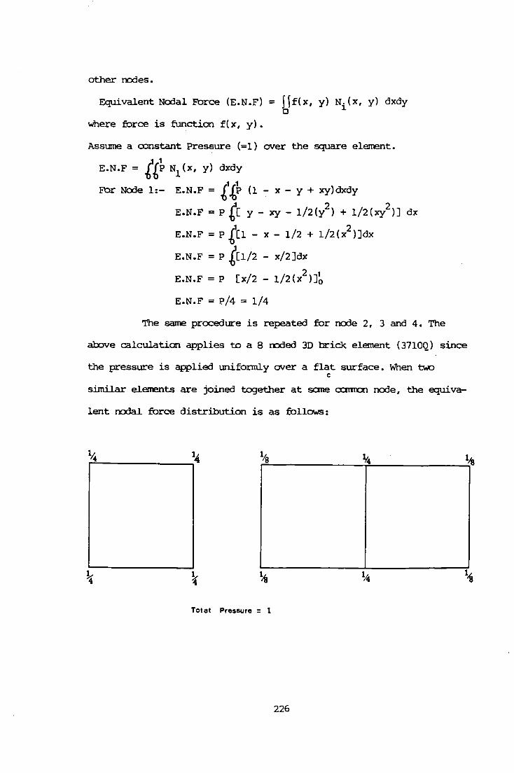
other nodes.

Equivalent Nodal Force (E. N. F) = jlf(x, y) N. (x, y) dxdy CJ ~

where force is function f(x, y).

Assume a o:mstant Pressure (=1) CNer the square element.

E.N.F = t£~ N1 (x, y) dxdy

~ 1 For Node 1:- E.N.F = £ ~p (1 - JC - y + xy)dxdy

E.N.F = P Cc y- xy- 1/2(y2 l + 1/2(xy

2 )J dx

E.N.F = P t[1 - x- 1/2 + 1/2(x2

)]dx

E.N.F = P t[l/2 - x/2]dJC

E.N.F = P [x/2 - l/2(x2 )]~

E.N.F = P/4 = 1/4

The same procedure is repeated for node 2, 3 and 4. The

ab:Jve calculation applies to a 8 noded 3D brick element ( 3710Q) since

the pressure is applied uniformly CNer a flat surface. When 0.0 c

similar elements are joined together at sane a:amca1 node, the 6:Illiva-

lent nodal force distribution is as follows:

1;.4 1~ r---------,"1 lie

Total Pressure = 1

226

APPENDIX II • CCNTAcr AREA AND PRESSURE BE'I'WEEN THE TYRE

AND THE RJAD.

There is general agrePJnent among investigators that the

contact area under the wheels on the flexible pavement is approxi.rrate-

ly elliptical. The pnetnnatic tyres on which virtually all road vehicl-

es rrove do not apply a uniform contact pressure over a circular area

of the road surface as is generally assumed in the analysis of multi-

layer elastic systems. For 1mloaded conditions, the envelope of the

contact area of tyres closely approximates to circles. At full load

the tyre walls define the edge of a parallel sided oval of length

breath ratio of about 1.4, while over loading results in further

elongation of the envelope between the tyre walls ( 26 ) .

Lister (26) has reported that an approxi.rrately a:mstant

a:mtact area is maintained for full load a:mditions over the range of

recammended inflation pressure p but no general relation exists - p

between this actual contact area, A , and the a::mp1ted area, A , c p

defined by W/P , where W is the static wheel load. He reported that p

it is reasonable to assume that for load ratios:

(actual wheel load)

( reccmnended wheel load )

of the order 0.5, the tyre mntact area is reasonably circular and the

a:mtact pressure across it is parabolic in form. The loaded area is a

parallel sided oval under a fairly uniform distribution of pressure,

and under overloaded mnditions, the envelope is elongated towards a

length/breadth ratio of 2:1 with peak mntact pressures under the side

walls and with flat longitudinal profiles. Fig A.l shows the change of

lateral profile of contact pressure with inflation pressure (26).

227

These loading conditions differ oonsiderably fran the usual

ass1..1ITif tion of a uniformly loaded circular -"\t:"l=~-"\ defined by (W/P ) p

i.e. static wheel load divided by the tyre inflation pressure.

However , Lister (26) found that making the assumption of circular

loading, results in errors of less than 2% when used to calculate

interfacial pavement stresses and surface deflection under the whole

range of tyre load conditions.

Sanborn et al (120) carried out a cx:mparison of stress and

displacement proouc:ed by a semi-elliptical loads and that proouc:ed by

uniform circular loads for varying depths and offsets. The semi-elli-

psoidal load distribution proouced significantly higher stresses at

shallow depth than did a uniform circular load of equal magnitude. At

sane-what greater depths, stresses were the same for toth distribution

of load. Semi-ellipsoidal loads also indicate larger displacement near

the surface than does the equivalent uniform circular loads.

1100

1000

900 Inflation pressure (kN/m2)

.... 800 E z 700 ~ ~

600 ~ .. a. 500 t; .!! c: 400 0

(.)

200

100

0 100 50 0 50 100

Distance from centre-line of tYre (mm)

Fig A.l Change of Lateral Profile of Contact Pressure with

Inflation Pressure (after Lister et al , Ref 26) .

228

APPENDIX III. PAFEC PRJGRAM OF THE 30 ~DEL.

229

CONTROL FULL. CONTROL

PHASE=1 , 2 phase=4 PHASE=6 PHASE=? PHASE=9 SAVE

BASE=4000000 SKIP. CHECK SKIP. VALIDATION

STRESS CONTROL. END

REPLACE. MODULE MATERIAL

MATERIAL. NUMBER 11 6 . 0E09 0 . 35 2300 12 2 . 0E08 0 . 35 2000 13 2 . OEOB 0 . 35 2000 14 10. 0E07 0 . 35 1700 1' 11 . 0E07 0 . 35 1700 16 24. OE07 0 . 35 1700 17 3~. 0E07 0 . 35 1700 18 50. OE07 0 . 35 1800 19 10. OE07 0 . 35 1800 END. OF. DATA

E

TITLE DEFLECTED SHAPE OF ROAD NODES

X Y Z 2 . 5 4 . 0 1 . 5 2 . 585 4 . 0 1. 5 2 . 66 4 . 0 1. 5 2 . 76 4 . 0 1 . 5 2 . 92 4 . 0 1. 5 3 . 12 4 . 0 1.5 3 . 34 4 . 0 1.5 3 . 59 4 . 0 1.5 3 . 84 4 . 0 1.5 4 . 09 4 . 0 1.5 4 . 34 4 . 0 1.5 4 . 6 4 . 0 1. 5 4 . 9 4 . 0 1. 5 ~. 16 4 . 0 1 . 5 5 . 41 4 . 0 1. 5 ' · 66 4 . 0 1. 5 5 . 91 4 . 0 1. 5 6 . 16 4 . 0 1. 5 6 . 38 4 . 0 1. 5 6 . '8 4 . 0 1. 5 6 . 74 4 . 0 1 . 5 6 . 84 4 . 0 1. 5 6 . 9154. 01.5 7 . 0 4 . 0 1 . 5 2 . ' 4 . 0 2. 425 2 . 585 4 . 0 2 . 425 2 . 66 4 . 0 2 . 425 2 . 76 4 . 0 2 . 425 2 . 92 4 . 0 2 . 425 3 . 12 4 . 0 2 . 425 3 . 34 4 . 0 2 . 425 3 . ~9 4 . 0 2 . 425 3 . 84 4 . 0 2 . 425 4 . 09 4 . 0 2 . 425 4 . 34 4 . 0 2 . 425 4 . 6 4 . 0 2 . 425 4 . 9 4 . 0 2 . 425

NU RO

230

:1. 1b 4. 0 2. 42:1 :1.41 4.0 2. 42:1 :1. bb 4.0 2. 42:1 :1.91 4.0 2. 42:1 b. 1b 4. 0 2. 42:1 b.3a 4.0 2. 42:1 b. :;a 4.0 2. 42:1 b. 74 4.0 2. 42:1 b.a4 4.0 2. 42:1 b. 91:1 4.0 2. 42:1 7.0 4.0 2.42:1 7.0 4.0 0.2 7.0 4.0 0.:14:1 7.0 4.0 o.a:;:; 7. 0 4. 0 I. 10:1 7. 0 4. 0 I. 2:1:1 7. 0 4. 0 I. 34 7.0 4.0 I. 42:1 7. 0 4. 0 I. :17:1 7. 0 4. 0 I. bb 7. 0 4.0 I. 74:1 7. 0 4. 0 I. a95 7.0 4.0 2.145 b. 915 4. 0 2. 145 2. 5 4.0 0.2 2. 5 4. 0 I. 41:; 2.:1 4.0 I. 5a5 2. :;a:; 4.0 o. 2 2. 5a5 4. 0 I. 415 2. 5a5 4. 0 I. :;a5 2. 5a5 4. 0 I. 745 2.bb 4.0 1. bb b.a4 4.0 0.2 b. a4 4.0 1.34 b. a4 4. 0 1.b6 b.915 4.0 0. 2 b. 915 4. 0 I. 25:1 b.915 4.0 1. 34 b. 915 4. 0 I. 425 b. 915 4. 0 1. 575 b. 91:1 4. 0 1. bb b. 915 4. 0 1. 745 2.bb 4.0 0.2 2.:1 3.9 0. 2 2. 5 3. 9 I. 415 2. 5 3.9 1. 5a5 2. 5 3.9 2. 425 2. 5a5 3. 9 0.2 2. 5a5 3. 9 1. 41 5 2. 5a5 3.9 1. 5 2. 5a5 3. 9 I. 5a5 2. 5a5 3. 9 I. 745 2. 5a5 3.9 2. 425 2.bb 3.9 0.2 2. bb 3. 9 1. 5 2. bb 3. 9 I. b6 2.bb 3.9 2.425 6. a4 3. 9 0.2 b. a4 3. 9 I. 34 b. a4 3. 9 1. 5 b. a4 3. 9 1. b6 b.a4 3. 9 2. 425 b.915 3.9 0. 2 b. 915 3. 9 I. 255 b. 915 3. 9 I. 425 b. 915 3. 9 1. 5

231

6.915 3.9 1. 575 6. 91~ 3. 9 l. 66 6. 915 3. 9 1. 745 6.915 3.9 2. 425 7.0 3.9 0.2 7. 0 3. 9 1. 255 7. 0 3. 9 1. 425 7. 0 3. 9 l. 575 7. 0 3. 9 1. 745 7.0 3.9 2.425 2.:1 3.6 0.2 2.5 3.6 2. 425 2.585 3.6 0.2 2.:18:13.6 1.415 2.:185 3.6 1. 5 2. 585 3. 6 1. 585 2. 585 3.6 1.745 2. 585 3.6 2. 425 2.66 3.6 0.2 2. 66 3. 6 l. 5 2.66 3.6 1.66 2.66 3.6 2.425 6.84 3.6 0.2 6.84 3.6 1.34 6.84 3.6 1. 5 6. 84 3. 6 l. 66 6.84 3.6 2.425 6.915 3.6 0.2 6.91:1 3.6 1.425 6. 915 3 .. 6 1. 5 6. 915 3. 6 l. 575 6.9153.61.66 6.915 3.6 2.425 7.0 3.6 0. 2 7.0 3.6 2. 425 2. 5 3.45 0.2 2. 5 3.45 2. 425 2. 585 3.45 0.2 2.585 3.45 1.415 2. 585 3. 45 1. 5 2. 585 3.45 1. 585 2. 585 3.45 1. 745 2. 585 3.45 2.425 2.66 3.45 0.2 2. 66 3. 45 l. 5 2.66 3.45 1.66 2.66 3.45 2.425 6.84 3.45 0.2 6.84 3.45 1.34 6.84 3.45 1. 5 6.84 3.45 1.66 6.84 3.45 2.425 6. 919 3. 45 0. 2 6.915 3. 45 1.425 6. 915 3. 45 1. 5 6.915 3.45 1. 575 6.915 3.45 1.66 6. 915 3.45 2.425 7.0 3.45 0. 2 7.0 3.45 2. 425 2. 5 3.076 0.2 2. 5 3.076 2.425 2. 585 3.076 0.2 2. 585 3.076 1.415 2. 585 3.076 1. 5 2. 585 3.076 1. 585

232

a.5B5 3.076 1.745 a. 585 3.076 a.425 a.66 3.076 0.2 2. 66 3. 076 1. 5 a.66 3.076 1.66 a.66 3.076 2. 425 6.84 3.076 0.2 6.84 3.076 1.34 6. 84 3. 076 1. 5 6.84 3.076 1.66 6.84 3.076 a.425 6.915 3.076 0.2 6.915 3.076 1.425 6. 915 3. 076 1. 5 6.915 3.076 1.575 6.915 3.076 1.66 6.915 3.076 a.4a5 7.0 3.076 0.2 7.0 3.076 a.4a5 a. 5 a. 702 0.2 a.5 a.702 a.425 2. 585 2. 702 0. 2 2.585 2.702 1.415 2. 585 2. 702 1. 5 2.585 2.702 1.585 2. 585 2.702 1.745 2. 585 2.702 2.425 2.66 2.702 0.2 2.66 a.702 1. 5 2.66 2. 702 1.66 2.66 a.702 2. 425 6.84 2. 702 0.2 6.84 2.702 1.34 6.84 2.702 1. 5 6.84 2. 702 1.66 6.84 2.702 2.425 6.915 2.702 0.2 6.915 2.702 1.425 6.915 2.702 1. 5 6.915 2. 702 1. 575 6.915 2.702 1.66 6.915 2. 702 2. 425 7.0 2. 702 0.2 7.0 2.702 a.425 2.5 2.328 0.2 2.5 2.328 2.425 2.58:5 2.328 0.2 2.58:5 2.328 1.41:5 2. 585 2. 328 1. 5 2 .. :58:5 2. 328 1. :58:5 2. 585 2.328 1.745 2.585 2.328 2.425 2.66 2.328 0.2 2.66 2.328 1. 5 2. 66 2. 328 1. 66 2.66 2.328 2.425 6.84 2.328 0.2 6. 84 2. 328 1. 34 6.84 2.328 1. 5 6. 84 2. 328 1. 66 6.84 2.328 2. 425 6.91:5 2.328 0.2 6.915 2.328 1. 425 6. 915 2. 328 1. 5 6.915 2.328 1. 575 6.91:5 2.328 1.66

233

6.915 2.328 2. 425 7.0 2. 326 0. 2 7.0 2. 326 2. 425 2. 5 l. 954 0. 2 2. 5 l. 954 2. 425 2. 585 l. 954 0. 2 2. 585 1.954 1. 415 2. 585 I. 954 l. 5 2. 585 1.954 1. 585 2. 585 1.954 1. 745 2. 585 1. 954 2. 425 2. 66 l. 954 0.2 2.66 l. 954 l. 5 2.66 1. 954 l. 66 2.66 1. 954 2. 425 6.84 1. 954 0. 2 6.84 l. 954 1. 34 6.84 1. 954 1. 5 6.84 1. 954 l. 66 6.84 1. 954 2. 425 6.915 1. 954 0. 2 6. 915 1. 954 1. 425 6.915 1. 954 1.5 6.915 l. 954 1. 575 6.915 1. 954 l. 66 6.915 1. 954 2. 425 7. 0 l. 954 0. 2 7. 0 l. 954 2. 425 2. 5 I. 58 0. 2 2. 5 l. 58 2. 425 2. 585 I. 58 0. 2 2. 585 I. 58 I. 415 2. 585 I. 58 1.5 2. 585 I. 58 l. 585 2. 585 I. 58 I. 745 2. 585 I. 58 2. 425 2.66 l. 58 0.2 2.66 I. 58 I. 5 2.66 l. 58 I. 66 2.66 l. 58 2. 425 6. 84 l. 58 0.2 6. 84 l. 58 1. 34 6.84 l. 58 1.5 6. 84 1. 58 I. 66 6.84 1. 58 2. 425 6. 915 l. 58 0. 2 6.915 1. 58 1.425 6. 915 l. 58 I. 5 6.915 1. 58 1. 575 6. 915 1. 58 I. 66 6.915 1. 58 2.425 7. 0 l. 58 0. 2 7. 0 1. 58 2. 425 2. 585 4. 0 l. 255 2. 66 4. 0 l. 34 2. :18:1 3. 9 l. 255 2. 66 3. 9 1. 34 6. 91 5 3. 9 I. 34 2. 585 3. 6 I. 255 2. 66 3.6 1. 34 6. 91 5 3. 6 1. 34 2. 585 3. 45 I. 255 2. 66 3. 45 I. 34 6. 915 3. 45 l. 34 2. 585 3. 076 1. 255 2. 66 3. 076 l. 34

234

6. 915 3. 076 I. 34 2. 585 2. 702 I. 255 2. 66 2. 702 I. 34 6.915 2. 702 1.34 2. 585 2.328 1.255 2. 66 2. 328 I. 34 6. 915 2. 328 1. 34 2. 585 1.954 1. 255 2. 66 I. 954 I. 34 6. 915 1.954 1.34 2. 585 I. 58 1. 255 2. 66 I. 58 I. 34 6. 915 I. 58 I. 34 2. 66 4. 0 I. 255 2. 66 3. 9 I. 255 2.66 4.0 I. 745 2.66 3.9 I. 745 2. 66 3.6 1. 255 2. 66 3. 6 I. 745 2. 66 3. 45 I. 255 2. 66 3. 45 I. 745 2.66 3.076 I. 255 2. 66 3.076 1. 745 2.66 2. 702 1.255 2.66 2. 702 I. 745 2.66 2. 328 1.255 2.66 2. 328 1. 745 2.66 1.954 1.255 2.66 1.954 I. 745 2. 66 1. 58 I. 255 2.66 1.58 1.745 2. 5 I. 206 0. 2 2. 5 I. 206 2. 425 2. 585 I. 206 0. 2 2. 585 1.206 1.255 2. 585 1.206 1.415 2. 585 I. 206 I. 5 2. 585 1.206 I. 585 2. 585 1. 206 I. 745 2. 585 1. 206 2. 425 2. 66 I. 206 0. 2 2.66 1. 206 1.255 2. 66 I. 206 I. 34 2. 66 1. 206 I. 5 2. 66 1. 206 I. 66 2.66 1.206 1. 745 2.66 1. 206 2. 425 6. 84 I. 206 0. 2 6. 84 1. 206 I. 34 6. 84 I. 206 I. 5 6. 74 1. 206 1. 5 6. 84 I. 206 I. 66 6.84 1.206 2. 425 6. 915 1. 206 0. 2 6.915 1. 206 1.34 6.915 1. 206 1. 425 6. 915 1. 206 I. 5 6.915 I. 206 1. 575 6. 915 1.206 I. 66 6. 915 1.206 2. 425 7. 0 I. 206 0. 2 7. 0 1. 206 2. 425 PAFBLOCKS BLOCK. NUMBER TYPE ELEMENT. TYPE PROPERTIES NI N2 N3 N5 TOPOLOGY 1 I 37100 11 I 1 0 3 81 85 82 86 62 65 63 66 2 I 37100 11 I I 0 2 63 66 64 67 82 86 83 88

235

3 1 37100 11 1 0 4 83 88 84 90 64 67 25 26 4 1 37100 11 0 9 85 91 291 316 65 80 289 315 5 1 37100 11 0 1 291 316 86 292 289 315 66 290 6 2 37200 11 1 1 292 86 92 290 66 3 7 2 37200 11 1 1 1 1 86 87 92 66 2 3 8 2 37200 11 1 1 1 87 92 88 2 3 67 9 2 37200 11 1 1 1 92 88 93 3 67 69 10 37100 11 1 0 1 88 93 89 318 67 69 68 317 11 37100 11 1 0 10 89 318 90 94 68 317 26 27 12 37100 11 6 1 0 7 91 95 94 99 eo 70 27 46 13 1 37100 11 0 8 95 100 96 293 70 73 71 75 ;4 1 37100 11 0 1 96 293 97 102 71 75 22 76 15 2 37200 11 1 1 102 97 103 76 22 23 16 2 37200 11 1 1 97 103 104 22 23 77 17 37100 11 0 1 97 104 98 105 22 77 72 78 18 37100 11 1 0 5 98 105 99 107 72 78 46 47 19 37100 11 1 0 9 100 108 101 109 73 49 74 53 20 37100 11 1 0 2 74 53 76 ss 101 109 102 110 21 1 37100 11 0 2 102 110 104 111 76 55 77 56 22 1 37100 11 0 2 77 56 79 58 104 111 106 112 23 1 37100 11 0 10 106 112 107 113 79 58 47 48 24 1 37100 12 0 11 114 116 115 121 81 85 84 90 25 1 37100 12 0 9 116 122 294 319 85 91 291 316 26 1 37100 12 0 1 294 319 117 295 291 316 86 292 27 2 37200 12 295 117 123 292 86 92 28 2 37200 12 117 118 123 86 87 92 29 2 37200 12 1 118 123 119 87 92 88 30 2 37200 12 1 1 123 119 124 92 88 93 31 37100 12 1 0 1 119 124 120 320 88 93 89 318 32 37100 12 1 0 10 120 320 121 125 89 318 90 94 33 1 37100 12 6 1 0 7 122 126 125 130 91 95 94 99 34 1 37100 12 1 1 0 8 126 131 127 296 95 100 96 293 35 1 37100 12 1 0 1 127 296 128 132 96 293 97 102 36 2 37200 12 1 132 128 133 102 .97 103 37 37100 12 1 0 1 128 133 129 134 97 103 98 104 38 37100 12 1 0 1 128 134 129 135 97 104 98 105 39 37100 12 0 5 129 135 130 136 98 105 99 107 40 37100 12 0 12 131 137 136 138 100 108 107 113 41 37100 13 0 11 139 141 140 146 114 116 115 121 42 1 37100 13 0 9 141 147 297 321 116 122 294 319 43 1 37100 13 0 1 297 321 142 298 294 319 117 295 44 2 37200 13 1 1 298 142 148 295 117 123 45 2 37200 13 1 1 142 143 148 117 118 123 46 2 37200 13 1 1 143 148 144 118 123 119 47 2 37200 13 1 1 148 144 149 123 119 124 48 1 37100 13 1 0 1 144 149 145 322 119 124 120 320 49 1 37100 13 1 0 10 145 322 146 150 120 320 121 125 50 1 37100 13 6 0 7 147 151 150 !SS 122 126 125 130 51 1 37100 13 0 8 151 156 !52 299 126 131 127 296 52 1 37100 13 0 152 299 !53 157 127 296 128 132 53 2 37200 13 1 1 157 153 158 132 128 133 54 2 37200 13 1 1 153 158 159 128 133 134 55 37100 13 1 0 1 153 !59 154 160 128 134 129 135 56 37100 13 0 s 154 160 !SS 161 129 135 130 136 57 37100" 13 0 12 156 162 161 163 131 137 136 138 58 37100 14 0 11 164 166 165 171 139 141 140 146 :59 1 37100 14 1 0 9 166 172 300 323 141 147 297 321 60 1 37100 14 0 1 300 323 167 301 297 321 142 298 61 2 37200 14 1 1 1 301 167 173 298 142 148 62 2 37200 14 1 1 1 167 168 173 142 143 148 63 2 37200 14 1 1 168 173 169 143 148 144 64 2 37200 14 1 1 173 169 174 148 144 149 65 1 37100 14 1 0 1 169 174 170 324 144 149 145 322 66 37100 14 1 0 10 170 324 171 175 145 322 146 150 67 37100 14 6 0 7 172 176 175 180 147 151 150 155 68 1 37100 14 1 1 0 8 176 181 177 302 151 156 152 299

236

69 1 37100 14 1 0 1 177 302 178 182 152 299 153 157 70 2 37200 14 1 1 1 1 182 178 183 157 153 158 71 2 37200 14 1 1 1 1 178 183 184 153 158 159 72 1 37100 14 1 1 0 1 178 184 179 185 153 159 154 160 73 1 37100 14 1 1 0 5 179 185 180 186 154 100 155 161 74 1 37100 14 1 1 0 12 181 187 186 188 156 162 161 163 75 1 37100 15 1 1 0 11 189 191 190 196 164 166 165 171 76 1 37100 15 1 1 0 9 191 197 303 325 166 172 300 323 77 1 37100 15 1 1 0 1 303 325 192 304 300 323 167 301 78 2 37200 15 1 1 1 1 304 192 198 301 167 173 79 2 37200 15 1 1 1 1 192 193 198 167 168 173 eo 2 37200 15 1 1 1 1 193 198 194 168 173 169 81 2 37200 15 1 1 1 1 198 194 199 173 169 174 82 1 37100 15 1 1 0 1 194 199 195 326 169 174 170 324 83 1 37100 15 1 1 0 10 195 326 196 200 170 324 171 175 84 1 37100 15 6 1 0 7 197 201 200 205 172 176 175 180 85 1 37100 15 1 1 0 8 201 206 202 305 176 181 177 302 86 1 37100 15 1 1 0 1 202 305 203 207 177 302 178 182 87 2 37200 15 1 1 1 1 207 203 208 182 178 183 88 2 37200 15 1 1 1 1 208 203 209 183 178 184 89 1 37100 15 1 1 0 1 203 209 204 210 178 184 179 185 90 1 37100 15 1 1 0 5 204 210 205 211 179 185 180 186 91 1 37100 15 1 1 0 12 206 212 211 213 181 187 186 188 92 1 37100 16 1 1 0 11 214 216 215 221 189 191 190 196 93 1 37100 16 1 1 0 9 216 222 306 327 191 197 303 325 94 1 37100 16 1 1 0 1 306 327 217 307 303 325 192 304 95 2 37200 16 1 1 1 1 307 217 223 304 192 198 96 2 37200 16 1 1 1 1 217 218 223 192 193 198 97 2 37200 16 1 1 1 1 218 223 219 193 198 194 98 2 37200 16 1 1 1 1 223 219 224 198 194 199 99 1 37100 16 1 I 0 1 219 224 220 328 194 199 195 326 100 1 37100 16 1 1 0 10 220 328 221 225 195 326 196 200 101 1 37100 16 6 1 0 7 222 226 225 230 197 201 200 205 102 1 3710o 16 1 1 o a 226 231 227 3oe 201 206 202 305 103 1 37100 16 1 1 0 1 227 308 228 232 202 305 203 207 104 2 37200 16 1 1 1 1 232 228 233 207 203 208 105 2 37200 16 1 1 1 1 228 233 234 203 208 209 106 1 37100 16 1 1 0 1 228 234 229 235 203 209 204 210 107 1 37100 16 1 1 0 5 229 235 230 236 204 210 205 211 108 1 37100 16 1 1 0 12 231 237 236 238 206 212 211 213 109 1 37100 17 1 1 0 11 239 241 240 246 214 216 215 221 110 1 37100 17 1 1 0 9 241 247 309 329 216 222 306 327 111 1 37100 17 1 1 0 1 309 329 242 310 306 327 217 307 112 2 37200 17 1 1 1 1 310 242 248 307 217 223 113 2 37200 17 1 l l 1 242 243 248 217 218 223 114 2 37200 17 1 1 1 1 243 248 244 218 223 219 115 2 37200 17 1 1 1 1 248 244 249 223 219 224 116 1 37100 17 1 1 0 1 244 249 245 330 219 224 220 328 117 1 37100 17 1 1 0 10 245 330 246 250 220 328 221 225 118 1 37100 17 6 1 0 7 247 251 250 255 222 226 225 230 119 1 37100 17 1 1 0 8 251 256 252 311 226 231 227 308 120 1 37100 17 1 1 0 1 252 311 253 257 227 308 228 232 121 2 37200 17 1 1 1 1 257 253 258 232 228 233 122 2 37200 17 1 1 1 1 253 258 259 228 233 234 123 1 37100 17 1 1 0 1 253 259 254 260 228 234 229 235 124 1 37100 17 1 1 0 5 254 260 255 261 229 235 230 236 125 1 37100 17 1 1 0 12 256 262 261 263 231 237 236 238 126 1 37100 18 1 1 0 11 264 266 265 271 239 241 240 246 127 1 37100 18 1 1 0 9 266 272 312 331 241 247 309 329 128 1 37100 18 1 1 0 1 312 331 267 313 309 329 242 310 129 2 37200 18 1 1 l 1 313 267 273 310 242 248 130 2 37200 18 1 l 1 1 267 268 273 242 243 248 131 2 37200 18 1 l 1 i 268 273 269 243 248 244 132 2 37200 18 1 I 1 1 273 269 274 248 244 249 133 1 37100 18 1 1 0 1 269 274 270 332 244 249 245 330 134 1 37100 18 1 1 0 10 270 332 271 275 245 330 246 250

237

135 37100 18 6 1 0 7 272 276 275 280 247 251 250 255 136 I 37100 18 I 0 8 276 281 277 314 251 256 252 311 137 I 37100 18 1 0 1 277 314 278 282 252 311 253 257 138 2 37200 18 1 282 278 283 257 253 258 139 2 37200 18 1 278 283 284 253 258 259 140 1 37100 18 0 278 284 279 285 253 259 254 260 141 I 37100 18 I 0 5 279 285 280 286 254 260 255 261 142 I 37100 18 1 I 0 12 281 287 286 288 256 262 261 263 143 I 37100 19 I 0 11 333 335 334 341 264 266 265 271 144 I 37100 19 I 0 9 335 342 336 343 266 272 312 331 145 I 37100 19 I 0 I 336 343 337 344 312 331 267 313 146 2 37200 19 I I I I 344 337 345 313 267 273 147 2 37200 19 I I I 337 338 345 267 268 273 148 2 37200 19 I I I 338 345 339 268 273 269 149 2 37200 19 I I I 345 339 346 273 269 274 ISO I 37100 19 I I 0 I 339 346 340 347 269 274 270 332 151 I 37100 19 I I 0 10 340 347 341 348 270 332 271 275 152 I 37100 19 6 I 0 7 342 349 348 354 272 276 275 280 153 I 37100 19 I I 0 8 349 355 350 356 276 281 277 314 154 I 37100 19 I 0 350 356 351 357 277 314 278 282 155 2 37200 19 I 1 357 351 358 282 278 283 156 2 37200 19 1 1 351 358 359 .278 283 284 157 37100 19 0 351 359 353 360 278 284 279 285 158 37100 19 0 5 353 360 354 361 279 285 280 286 159 1 37100 19 0 12 355 362 361 363 281 287 286 288 MESH REFERENCE SPACING. LIST 1 1 2 2 3 2. 3 2.06667 1. 66667 1 1. 06667 4 1. 06667 1 1. 66667 1. 86667 5 1 1. 76471 2.94118 3. 29412 6 I 1. 6 2 2.2 2. 52.5 2. 52.5 2. 6 7 4. 05882 3. 64706 2. 94118 I. 76471 •3.29412 8 4. 05882 3.64706 2.94118 I. 76471 9 2. 3 2.06667 1. 66667 I 10 1 I. 66667 I. 86667

3 2. 6 2. 5 1. 88235

11 4.05882 3. 64706 2.94118 I. 76471 1.88235 •2.94118 3. 29418

2. 5 2. 5 2. 5 2.2 2 I. 88235 I 1. 76471

I 1. 88235 1. 76471

1.6 I 2. 94118

12 4.6 4.13333 3. 33333 2 I. 13333 I. 13333 I •3. 73333

1. 13333 1. 13333 2 3. 33333

MATERIAL MATERIAL. NUMBER E NU

11 6.0E09 0.35 2300 12 2.0EOB 0.35 2000 13 2. OEOB 0. 35 2000 14 6. OE07 0. 35 1700 15 11.0E07 0. 35 1700 16 24.0E07 0.35 1700 17 35.0E07 0. 35 1700 18 50.0E07 0. 35 1800 19 100. OE07 0.35 1800 PRESSURE LOAD. CASE PRESSURE. VALUE LIST. OF. NODES 1 7. 73E05 63 66 64 67 I 5. 77E05 74 53 76 55 77 56 79 58 STRESS. ELEMENT LIST 251 252 253 254 255 256 765

238

RO

766 767 768 769 770 771 772 773 774 77'j 776 777 RESTRAINTS NODE.NUMDER 333 2 123 362 2 123 334 2 123 363 2 123 333 1 1 334 1 1 362 1 1 363 1 1 334 3 3 363 3 3 IN. DRAW

PLANE DIRECTION

DRAW TYPE INFO ORIE SIZE 1 3 0 4 I

OUT. DRAW DRAW PLOT ORIE SIZE

1 1 4 1 END. OF. DATA

239

APPENDIX rJ. TRANS • F77 •

240

c * c * c " c * c * c * c * c * c ... c .. c * c .. c * c * c ... c * c * c ... c ... c * c ... c * c * c .. c * c * c ... c * c ..

PROGRAM TRANS.F77

THIS PROGRAM TRANSFERS THE DATAS FROM THE "PAFEC" OUTPUT FILE CALLED "0< __ >7",TO ANOTHER SPECIFIED FILE. THIS PROGRAM TRANSFER THE X VALUES <THE DISTANCE ALONG THE ROADl,DEFLECTION OF THE NEAR SIDE REAR WHEELS PATHS AND THE DEFLECTION OF THE MIDDLE OF THE LANE.

COLUMN

1 2 3 4

INFORMATION

X VALUES !Ml DEFL. OF. WHEEL PAT~ !mml DEFL. OF. MID-LANE !mml ** LINE NUMBER

** THE LINE NUMBER PROVIDES A MEAN TO DETECT THE END OF DATA WHEN USED IN ANOTHER PROGRAM,CALLED"DEFL.F77",WHICH CHANGES THE ABSLOUTE DEFLECTION INTO DEFLECTOGRAPH DEFLECTION. THE LAST LINE!NO 24liS GIVEN A VALUE 0 IN ORDER TO CARRY OUT THE ABOVE TASK.

TO RUN THE PROGRAM.PLEASE TYPE THE FOLLOWING COMMANDS:-

$77 TRANS -IN •>PAFEC2>0MDTH7 -OUT PMDTH7

ASSUMED:- 1lPAFEC OUTPUT FILE =OMDTH7 ------ 2lTRANSFERED OUTPUT FILE = PMDTH7

3lFILE = OMDTH7 IS IN THE Sub-UFD CALLED PAFEC2

...

...

...

... .. .. * .. .. .. .. ... .. .. .. .. * .. .. .. .. ... .. .. .. .. .. .. ...

c ***************************************************************************** c

c

PROGRAM TRANS DIMENSION X!3Ql,YAAD!30l.YBAD!30l.K!30l REAL *B C,YAAD.YBAD. X INTEGER I.K

C THESE STATEMENTS SKIPS THE FIRST 64 LINES.

c

DD 10. 1=1, 64 READ 15. 161

15 FORMAT !A20l 10 CONTINUE

C THESE STATEMENTS PICKS UP THE MULTIPLICATION FACTOR. READ 15, 161 C

16 FORMAT !29X,E6. Ol c C THESE STATEMENTS SKIPS THE NEXT 3 LINES.

c

DO 20. I=1.3 READ (5, 151

20 CONTINUE

C THESE STATEMENTS PICKS UP THE FIRST 24 DEFLECTIOS<WHEEL PATH! AND THE X C VALUES.

c

DO 50. I=1, 24 READ (5,301 YAAD!I), XIII

30 FORMAT !19X,F9. 3,45X,F5.2l

C THIS STATEMENT DIVIDES THE DEFLECTIONS BY THE MULTIPLICATION FACTOR AND C THEN CHANGE THE DEFLECTION FROM M TO mm.

YAAD!Il=!YAAD!Il/Clo1QOO.O c

50 CONTINUE c C THESE STATEMENTS PICKS UP THE SECOND 24 SETS OF DEFLECTIONS!MID-LANEl.

DO 60, I= I. 24

241

c

READ (5,40) YBAD<Il 40 FORMAT C19X,F9. 3)

C THIS STATEMENT DIVIDES THE DEFLECTIONS BY THE MULTIPLICATION FACTOR AND THEN C CHANGES THE DEFLECTIONS FROM M TO mm.

YBAD<Il=CYBAD<Il/Cl*1000. 0 c

60 CONTINUE c C THESE STATEMENTS NUMBER THE LINES 1 TO 24. LINE 24 IS GIVEN THE NUMBER 0.

c

DO 18 I=1,24 KCil=I

18 CONTINUE KC24)cQ

C THESE STATEMENTS PRINTS THE RESULTS IN THE FOLLOWING ORDER; X VALUES, C DEFLECTIONS<WHEEL PATH), DEFLECTIONSCMID-LANEl AND LINE NUMBER

c

c

DO eo. I=1.24 WRITE (6,70) XCil,YAADCil,YBADCil,KCil

70 FORMAT CSX,FS. 2, 10X,2PE12. 4, 10X.2PE12. 4, !OX, 13)

80 CONTINUE

STOP END

242

APPENDIX V. PI.JJr. F77 •

243

c ********•******************************************************************* C * PROGRAM PLOT.F77 * c * ---------------- * c * * c * c * c * c * c * c * c * c * c * c * c .. c * c .. c " c * c * c * c * c. .. c .. c .. c .. c .. c ..

THIS PROGRAM CHANGES THE ABSOLUTE DEFLECTION INTO DEFLECTOGRAPH DEFLECTION.

LENGTH OF LONG ARM<T DATUM FRAME) LENGTH OF SHORT ARM!BEAM> RATIO <L2/L1) < 1-<L2/Ll l l

B = TIP OF T-DATUM FRAME A HEAD OF BEAM FRAME C TIP OF BEAM FRAME

XADCO = ORGINAL POSITION OF C XADBO = ORGINAL POSITION OF B XADAO = ORGINAL POSITION OF A

XADCT FINAL POSITION OF C XADBT = FINAL POSITION OF B XADAT FINAL POSITION OF A

L1 L2

2130MM 1530MM. 0. 7183MM 0.2187MM

XAD = DISTANCE ALONG THE ROAD FOR ABSOLUTE DEFL. XAA DISTANCE ALONG THE ROAD FOR DEFLECTOGRAPH DEFL

YAAD = DEFLECTION<ABS> OF ROAD ALONG THE BEAM YBAD = DEFLECTION<ABSl OF ROAD ALONG THE T-DATUM FRAME YAA = DEFLECTION<DEFLIOGRAPH> OF THE ROAD ALONG THE

* * * * * * .. .. .. .. .. .. .. * .. * .. * .. .. .. .. .. ..

C * BEAM OF THE NEAR SIDE WHEELS * c .. * C * XAD 7. 0 POSITION OF THE CENTRE OF REAR WHEELS * C * XAD = 2. 5 POSITION OF THE CETREE OF FRONT WHEEL * c * * C * DEFLECTOGRAPH DEFLECTIONS CAN ONLY BE GIVEN AT FOLLOWING INTERVALS:- * C * SO, 100, 125, 200 AND 250mm * c .. .. c .. *

COMMAND:- .. .. c .. c .. c .. c .. c ..

TO RUN TYPE THE FOLLOWING SF77 PLOT PMDTH6 <WHEN SMDTH6 <WHEN

YOU YOU . )

YOU

ARE ASKED FOR THE NAME OF THE DATA FILE. ) * ARE ASKED FOR THE NAME OF THE OUTPUT *

c * c .. c .. c ..

FILE 100 !WHEN ARE ASKED FOR THE INTERVAL. )

ASSUMED:-1lDATA FILE NAME PMDTH6 2lOUTPUT FILE NAME = SMDTH6

* .. .. * ..

C * 31 INTERVAL = 100mm * c * .. c **************************************************************************** c

c

PROGRAM PLOT DIMENSION XAD<400l,YAAD<400l,YBAD<400l LOGICAL +2 QU CHARACTER +20 FILONE.FILTWO

C DECLARE VARIABLES AS REAL

c

REAL +4 XDD.YDD, XADCT,YADCT, XADCO,YADCO. XADBT.YADBT, XADBO.YADBO, *XADAT,YADAT, XADAO,YADAO, XAD,YAAD,YBAD.MAX,MIN• INT, INTER

C DECLARE SOME INTEGERS. INTEGER *4 I,K,M

c C ENTER THE DATA FILE NAME WHEN YOU ARE ASKED

1 PRINT *• 'PLEASE ENTER THE NAME OF THE DATA FILE' READ (+,2) FILONE

2 FORMAT <A20l

244

c C CHECK IF THE NAMED DATA FILE EXISTS

INOUIRE<FILE=FILONE,EXIST=QU) IF!QU) GO TO 3

c C IF THE DATA FILE DOES NOT EXISTS THEN

c

PRINT *• 'FILE NOT FOUND! PLEASE TRY AGAIN' GO TO I

C IF THE NAMED DATA FILE EXISTS THEN

c

3 PRINT *• 'PLEASE ENTER THE NAME OF THE OUTPUT FILE ' READ <•,2> FILTWO

C ENTER THE INTERVAL! 50, 100, 125 OR 200 mm> OF THE DEFLECTOGRAPH READING C REQUIRED

PRINT *• 'INTERVAL! 50, 100, 125,200 OR 250 mm)' READ (+,5) INTER

5 FORMAT !F6.0) C TO OPEN THE OUTPUT FILE

OPEN!6,FILE=FILTWO.STATUS='UNKNOWN'> c

c

WRITE !6, Bl) Bl FORMAT < 2BX, '------------' )

WRITE (6,B2) B2 FORMAT !2BX, 'IDEFLECTION: ')

WRITE !6.B3) B3 FORMAT !2BX. '------------•, 1//)

WRITE (6,94> 94 FORMAT !6X, 'NOTE', /,6X, '----•, I>

WRITE !6,93) 93 FORMAT !6X, 'MEA. DEFL = DEFLECTOGRAPH DEFLECTIONS MEASURED. ', /, 6X,'

•WHL. DEFL = ABSLOUTE DEFLECTIONS THROUGH THE REAR WHEELS. ', /, 6X, 'Ml +D.DEFL = ABSLOUTE DEFLECTIONS THROUGH THE MID-LANE.',///)

WRITE !6,B4> 84 FORMAT < 1 X, '------------------------- ', 12X, '-------------------- ' )

WRITE !6,85) BS FORMAT !IX, 'DEFLECTOGRAPH DEFLECTION', 13X, 'AIJSLOUTE DEFLECTION'>

WRITE <6.86> 86 FORMAT < 1 X, ·------------------------- ', 12X, •-------------------- ',

•n WRITE ( 6, B7>

87 FORMAT <3X. '------ '. 2x, '--------------',ex. '------ ', 2x, '-------------I I 3X. , ____________ ')

WRITE (6,8B) BB FORMAT !4.X, 'X(M) ', 4X, 'MEA. DEFL!mm) ',!OX, 'X!M) '• 4X, 'WHL. OEFL!mm) ', 3

+X, 'MID. DEFL<mm) ') WRITE (6, B9)

89 FOR,.,AT <3X, '------ ', 2X, '--------------', 8X, '------', 2X. '-------------',3X, '-------------'>

C TO PRINT THE DEFLECTOGRAPH AND ABSLOUTE DEFLECTIONS TOGETHER IN THE C SAME OUTPUT FILE<FILTWO>,THE SUBROUTINE CALLED "DATASO", IS USED. C THIS SUBROUTINE OPEN THE ORQINAL DATA FILE<FILONE> AND READS THE DATAS.

CALL OATASO<XAD,YAAD.YBAO.FlLONE> c C CHANGE INTERVAL TO METERS.

INT=<INTER/1000) c C NUMBER OF INTERVALS + I

N = <<1000/INTER>+I) c C SET 1=0 FOR PRINTING PURPOSE

1=0 c C OPEN n:~ MAIN LOOP FOR VARIOUS POINTS<X VALUES> ALONG THE ROAD, AT C SPECIFIED INTERVAL

245

C STARTION POINT OF INTERPLOTING. MAX=7. 0

C LAST POINT OF INTERPLOTION MIN=6.0

c

DD 10 XDD=MIN.MAX, INT XADCO=IXDD-0.991 XADAD=IXDD-2. 521 XADilO=IXDD-0.391 XADCT=IXDDI XADAT= C XDD-1. 53 I XADilT=CXDD+0.61

C SINCE THE ABSLOUTE DEFLECTIONS ON EITHER SIDE OF THE WHEEL IS ASSUMED C TO llE THE SAME,THEN THE DEFLECTION AT DISTANCE X llEHIND THE WHEEL C WOULD llE THE SAME AS THE DEFLECTION AT DISTANCE X INFRONT OF THE C WHEEL

c

IFIXADBT.GT. 7.01 THEN XADBT=<7.0-IIXDD+0.6l-7.0ll END IF

C USE THE SUBROUTINE, "WHEEL", TO INTERPLOTE FOR VARIOUS POINTS C ALONG THE ROAD THROUGH THE CENTRE OF THE WHEEL.

c

CALL WHEELCXADCO.YADCO,FILONEI CALL WHEELCXADCT.YADCT,FILONEl CALL WHEELIXADAO,YADAO,FILONEl CALL WHEELCXADAT,YADAT,FILONEI

C USE THE SUBROUTINE, "CENTRE", TO INTERPLOTE FOR VARIOUS POINTS C ALONG THE ROAD FOR THE CENTRE LINE OF THE CENTRE.

c

CALL CENTRECXADBO,YADilQ,FILONEl CALL CENTRECXADBT.YADilT.FlLONEl

C TO CHANGE ABSLOUTE DEFLECTIONS INTO DEFLECTOGRAPH DEFLECTIONS. YDD=<YADCT-YADCOl-CO. 71831•CYADilT-YADBOl-CO. 2817l*CYADAT-YADAOI

c C TO CHANGE REAL NUMBERSCNI TO INTERGERSCLI.

L=N C TO PRINT THE RESULTS DISTANCE<ALONG THE ROADI,DEFLECTOGRAPH AND C AllSLOUTE DEFLECTIONS.

1=1+1 IF C I. LE. Ll THEN WRITE C6, 151 XDD, YDD, XAD< I I, YAADI I I, YBADI I l

15 FORMAT C3X,F6. 3.3X,2PE10. 1, 11X,OPF5. 2,3X,2PE12. 4.3X,2PE12. 41 END IF

c C TO CLOSE THE MAIN LOOP

10 CONTINUE c C TO PRINT THE REMAINING SETS OF THE ABSLOUTE DEFLECTION:­

M=L+1

16 18

C TO

c

c

DO 18,K=M,24 WRITE C6, 161 XADCKI,YAADCKI,YBADCKI FORMAT C33X,F5.2,3X,2PE12. 4,3X,2PE12. 41

CONTINUE CLOSE THE OUTPUT FILECFILTWOI

CLOSEC61

STOP END

C SUBROUTINE, "WHEEL", LAYOUT. SUBROUTINE WHEELIXE,YE,FILONEI DIMENSION XADC400I,YAA0!4001 REAL •4 XAD,YAAD, XE.YE INTEGER !. .J, K CHARACTER •20 FILONE

246

c C TO OPEN THE DATA FILECFILONEI.

c

OPENC5,FILE=FILONE,STATUS='UNKNOWN'I I=l

C ALL THE LINES IN THE DATA FILE WILL HAVE A LINE NUMBER IN THE LAST C COLUMN EXCEPT FOR THE LAST LINE WHICH WILL HAVE A INTERGER=O. THIS C ENABLE THE END OF DATA TO BE DETECTED.

20 READ (5,41 XADCII,YAADCII,K 4 FORMAT C5X, F5. 2, !OX, E12. 4, 32X, !31

c I=l+l

c C THIS COMMANDS ENSURES THAT, I HAS NOT EXCEEDED 400<DIMENSION=4001.

IF<I.GT. 4001 STOP c C THIS COMMAND ENSURES THAT EACH DATA IS READ TILL THE LAST CARD WITH C INTEGER=O IS DETECTED.

IFCK.GT.Ol GO TO 20 c C CHECK FOR X VALUE LESS THAN SMALLEST XAD VALUE ON CURVE.

IFCXE. LT. XAD<lll STOP J=2

c C THE FOLLOWING ARITHMETIC IF STATEMENT COMPARES THE GIVEN X VALUE C WITH SUCCESSIVE VALUES ON THE CURVE,LOOKING FOR AN X VALUE ON THE C CURVE THAT IS GREATER THAN THE GIVEN VALUE.

25 IFCXE-XADCJII 40,35,30 c C NOT FOUND YET.

30 J=J+I c C CHECK WHETHER GIVEN X VALUE IS GREATER THAN LARGEST X ON CURVE.

IFCJ.LT. 11 GO TO 25 STOP

c C EQUAL

c

35 YE=YAAD<JI GO TO 100

C TWO CURVE VALUES BRACKET GIVEN X -- INTERPOLAE.

c

c

40 YE=YAADCJ-li+(YAADCJI-YAADCJ-111/CXADCJI-XADCJ-lii*(XE-XAD(J-111

100 CLOSEC51 RETURN END

C SUBROUTINE, "CENTRE", LAYOUT.

c

c

c

c

c

c

SUBROUTINE CENTRE<XE,YE,FILONEI DIMENSION XAD<400I,YBADC4001 REAL *4 XAD,YBAO, XE,YE INTEGER I,J,K CHARACTER •20 FILONE

OPENC5,FILE=FILONE.STATUS='UNKNOWN'I I=l

20 READ (5,41 XADCJI,YBADCII,K 4 FORMAT C 5X, F5. 2, 32X, E12. 4, !OX, 131.

I=l+l

IFCI. GT. 4001 STOP

IFCK. GT. Ol GO TO 20

247

c

c

c

c

c

c

c

IF<XE. LT. XAD!1) l STOP .J=2

25 IF<XE-XAD!Jl l 40.35.30

30 .J=.J+l

IF!.!. LT. Il GO TO 25 STOP

35 VE=VBAD!.Jl GO TO 100

40 VE=VBAD<.J-ll+!VBAD<Jl-YBAD<J-1))/(XAD<.Jl-XAD<J-1ll•<XE-XAD<.J-1ll

100 CLOSE!5l RETURN END

C SUBROUTINE. "DATASO",LAYOUT.

c

c

c

c

SUBROUTINE DATASO<XAD,YAAD,VBAD,FILONEl DIMENSION XAD!400l,VAAD!400l,VBAD<400l REAL •4 XAD,VAAD,VBAD INTEGER I CHARACTER *20 FILONE OPEN(5,FILE=FILONE,STATUS='UNKNOWN'l

DO 60, !=1, 24 READ (5,28> XAD<Il,YAAD<Il.VBAD<Il

28 FORMAT < 5X, F5. 2. lOX, E12. 4, lOX, E12. 4 l 60 CONTINUE

CLOSE<5l

RETURN END

c ************************************************************************

248

APPENDIX VI • TABLES OF STATISTICAL ANALYSIS OITA.U.S.

249

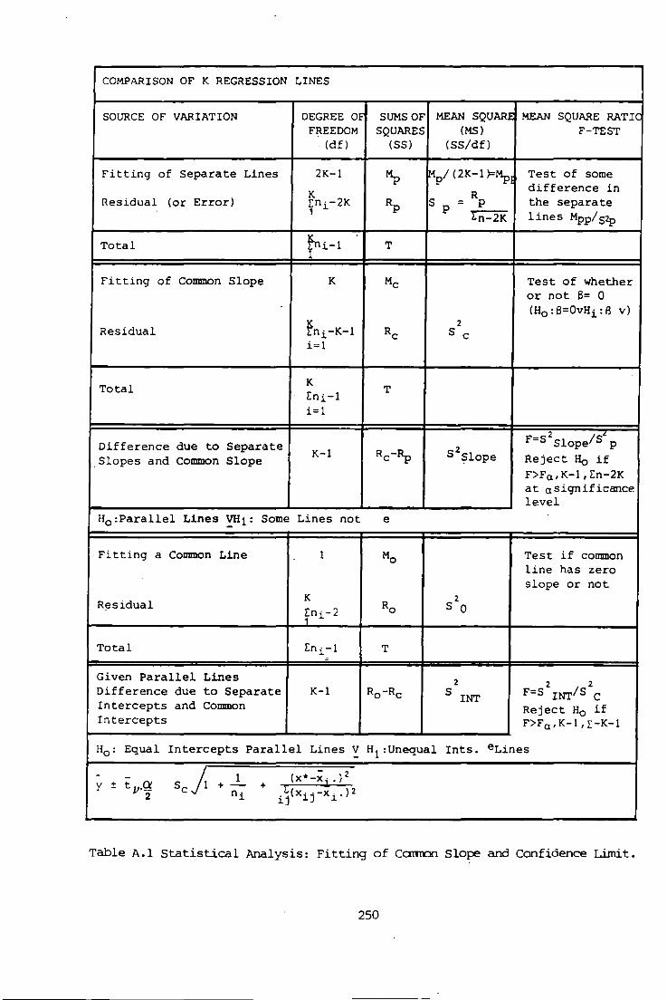
COMPARISON OF K REGRESSION LINES

SOURCE OF VARIATION DEGREE Of SUMS OF MEAN SQUARE MEAN SQUARE RATIC FREEDOM SQUARES (MS) F-TEST

. (df) (SS) (SS/df)

Fitting of Separate Lines 2K-1 f), MP/ (2K-1 )=~ Test of some

K R difference in

Residual (or Error) [n·-2K RP s p = p the separate 1 l.

tn-2K lines M pp/ S2p

Total fni-1 T

Fitting of Common Slope K Me Test of whether or not B= 0 (fio: B=OvHi: B v)

fni-K-1 2

Residual RC s c i=1

Total K T l:ni-1 i=1

Difference due to Separate K-1 2

F=S2slopels' P

.Slopes and Common Slope Re-~ S Slope Reject Ho if F>Fo., K-1, 1:n-2K at 0 significance level

H0 :Parallel Lines ~1: Some Lines not e

Fitting a Common Line 1 MO Test if common line has zero slope or not

Residual K 2 fni -2

Ro s 0

Total [ni -1 T -

Given Parallel Lines 2 2 2 Difference due to Separate K-1 Ro-Rc s F=S INT/S C INT Intercepts and Common Reject Ho if Intercepts F>F0 ,K-1,[-K-1

Ho: Equal Intercepts Parallel Lines V H1 :Unequal Ints. eLines -.

scp 1 - 2 (x•-x1 .)

y ± t jJ•g +- + i3(xij -xi. )2 2 ni

Table A.l Statistical Analysis: Fitting of CCl'lTl'OI'l Slope and Confidence Limit.

250

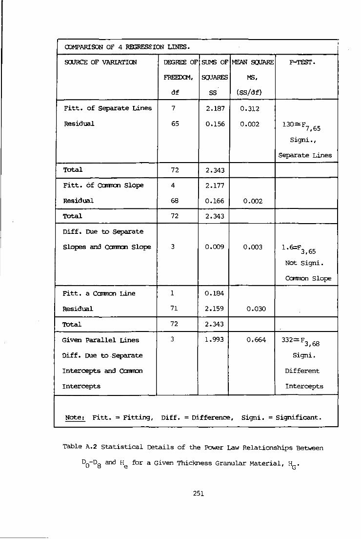
, <DMPARISON OF 4 RmRE'SS'ION LINES.

I

s:::uRCE OF VARIATICN DIDREE OF SUM) OF MEAN SOOARE F-TEST.

FREEDCM, SOJARES MS,

df ss (SS/df)

Fitt. of Separate Lines 7 2.187 0.312

Residual 65 0.156 0.002 130=F7,65

Signi.,

Separate Lines

Total 72 2.343

Fitt. of Qamman Slope 4 2.177

Residual 68 0.166 0.002

Total 72 2.343

Diff. Due to Separate

Slopes and Qamman Slope 3 0.009 0.003 1.6=F3, 65

Not Signi.

Carrron Slope

Fitt. a Ccmman Line 1 0.184

Residual 71 2.159 0.030

Total 72 2.343

Given Parallel Lines 3 1.993 0.664 332=F3, 68

Diff. Due to Separate Signi.

Intercepts and camcn Different

Intercepts Intercepts

Note: Fitt. = Fitting, Diff. = Difference, Signi. =Significant.

Table A.2 Statistical Details of the Pov.er Law Relationships Bet\o.€en

D0-D8 and He ~r a Given Thickness Granular Material, ~·

251

CBR H,.. rrm Equations no "

300 T..o:.:JlO (DO -08) = 1.679 - 2.346 T_,og10He 1\.l

2 500 LoglO(DO-D8) = 1.839 - 2.346 Log10r1e 3\.2

300 Logl.O(D0-08) - l 003 ·> 34" Log LT - • - ~ • '> lO""e A.. 3

10 500 LOglO(DO-D8) = 1.210 - 2. 346 Log1of-le .11..4 .

Table 1\.3 Equations to Describe the Relationships Between o0-o8

and H for a Given Value of Granular Material 'I'h.ickness, H,... e ·~

c:3R r\> m~ Equations No

400 Log10 (o0-o8 ) = l 688- ~.58') LoglOf-!e .11.. 5

2 600 LOg10 (o0-o8 ) = l.B30 - 2.585 LoglOHe 1\.6

400 Log10 (o0-o8 ) = 0.944- 2.585 LoglOHe 1\.7

10 600 Log10 (o0-o8 ) = 1.203 - 2.585 LoglOHe 1\.8

Table A.4 Gquations to Describe the Relationships Between o0-o3

and He for a Given Pavement Thickness, ~·

oCBI': E /E l 2 Equations No

40/2 Log10 (o0-o8 ) = 1.137 - 0.66 LoglOHe .'\. 9 '1 '- 100/2 Log10 (o0-o8 ) = 0.936 - 0.55 LoglOHe Jl •• 10

40/2 Log10 (o0-o8 ) = 0.974- 0.75 LoglOHe A.ll

10 100/2 Log10 (o0-o8 ) = 0.680- 0.56 LoglOHe .1\ .12

40/9 Log10 (o0-o8 ) = 0.950- 0.59 LoglOHe l\.13

2 100/9 Log10 (o0-o8 ) = 0.858- 0.52 LoglOH~ ;,.14

40/9 Log10 (o0-o8 ) = 1.201 - 1.44 Log10He A.l5

10 100/9 LoglO(DO-D8) = 0.764- 0.70 LoglOHe 1\.16

:~ 2 r. = f2

= X lO ~~/rrt w1

'l'·>i:.>le 1\.S Equations to Describe the Relationships Between o0-o8

and He for a Given Value of E1

/E2

Ratio.

252

E/E2 Equations No

100/2 LOg10 (o0-o2) = 3.145-1.221 LOg10H

1 A.l7

40/2 LOg10 (o0-o2 ) = 3.402-1.221 LOglOHl ;\.18

l00/9 LOglO(DO-D2) = 2. 970-1. 221 LOglOHl ]1 .. 19

40/9 LOg10 (o0-o2 ) = 3.200-1.221 LOglOHl A.20

2 E2 = El = x 108 N/m

'l'able A.6 Equations to Describe the Relationships Between o0-o2

and a1 fOr a Given Ratio of E1/E2•

Hl E2 Equations No

2 LOglO (D0-02) = 2.504 - 0.597 10g10s1 A.21

100 9 r..og

10(o

0-o

2 ) = 1.746-0.399 r..og10E

1 A.22

2 LOg10 (o0-o2

) = 2.734- 0.762 r..og10s1

A.23

150 g LOg10

(o0-o

2 ) = 2.337 - 0.680 LOg10

P.1

l\_, 24

H1 = rrm, 8 2 E2 = x 10 N/m •

Table A.7 Equations to Describe The Relationships Between o0-o2

and E1 fOr a given Value of E2 and H1 •

253

APPENDIX VII. TRIAXIAL TESTING.

A.l IntrOOuction.

To validate the pavement evaluation and design system set up

in Chapter 6. 0, requires Deflectograph deflection measurements togeth­

er with infonnation on the thickness and ll'Cldulus of the layerecfpaven­

ent with which to cnnpare predicted values of the layer properties.

cores of bituminous material were extracted fran local roads to deter­

mine the thickness and lalx>ratory triaxial testing was undertaken to

determine the ll'Cldulus of these layers.

A.2 Field Sampling.

Samples of bituminous material were collected fran local

roads, i.e. Totnes to Halwel (Road No.A381), where Deflectograph surv­

eys have been conducted previously. The thickness of the bituminous

material along these roads was not consistent but is usually less than

150 mn. A lOO mn core barrrel was used so that the thickness of the

sample is at least greater than the diameter of the sample. The height

of the sample should be greater than the diameter in order to obtain

stress-strain results free of the influence of end effects during

laboratory testing. The cores of bituminous material obtained were of

Dense Bituminous Macadam (D.B.M) with a layer thickness in the range

of 90 to 140 mn.

A.3 Sample Preparation and Platen Connection.

All the core samples were trimnecl at both ends using a dia!"Cl>­

nd tipped circular saw, so that the ends were srrooth and perpendicular

~54

to the sample axis. In conventional triaxial testing, where large

deformations are involved, it is often sufficiently accurate to use

the loading frame as a datum and to take measurements external to the

triaxial cell by llDI1itoring the rrovement of the load plunger. Hov.ever,

for dynamic repeated load testing, it is desirable to obtain measure­

ment directly on the sample. This procedure eliminates extraneous

defonnation in the system due to the sample end effects and sundry

!lDVements occurring externally 't:etween the cell base and the plunger

(132).

Very small holes were drilled in the. samples and six locating

targets, for measurement of longitudinal deformation, were secured

with glue to the sample at each end of the three gauge length. The

locating targets were spaced at 120 degrees of arc around the sample.

Two further small metal locating studs, diametrically opposite, were

secured with glue at the centre of the sample for measurement of

lateral defonnation.

A latex membrane was then placed over the sample necessitat­

ing the perforation of the membrane. The perforation was then sealed

to the locating targets with glue. A metal washer was then placed over

the locating targets and these were glued to the latex membrane.

Because of the small resilient deformations which were expec­

ted in these experiments, it was considered important that the _cylin­

drical samples remained cylindrical as long as possible during the

test (57). This can only 't:e achieved by providing "frictionless" end

platens whose diarnetersare greater than that of the sample. The nonun­

iformity of the stress distribution within the sample is pri.rrarily

due to the effects of the friction on the end plates. The radial disp­

lacement on the periphery at both ends varies inversely with a

255

friction factor ( 137 ) • The platens were !l'ade from ground and chraned,

hardened steel; tilese produce a law coefficient of friction. The coef­

ficient of friction was further reduced by using a sandwich of thin

rubber discs and silicone grease ( 138) • Lateral slipping of the sample

can occur with this form of testing due to slight inaccuracies of set­

ting up. To prevent excessive IlOVanent due to this lateral slipping a

S!l'all retaining lip in the base platen was inserted. The diameter of

tile retaining lip was slightly larger than the sample and the top

platen diameter.

A.S Stess Application 5ystem.

Vertical stress is applied to tile specimens by an hydraulic

actuator, see Plate A.L The actuator is controlled by closed serve

loops operating a serve valve on the actuator. A constant static load

is applied by setting tile o.c level of the reference signal at an

appropriate value. This "dead load" is introduced to represent tile

effects of overburden pressure in an actual road. The dynamic load in

either tile sinusoidal or triangular rrcx'le, is superi.mp.:>sed on this dead

load by selecting the required amplitude and frequency of the referen­

ce signal fran the function generator. This represents the effect of

tile wheel loads on the pavenent kno.r..n as 'live load' • The triaxial

cell is based on the design discussed by Bro.r..n et al (57, 132, 133) •

A.6 Measuring SyStem.

A.6.1 Applied Vertical LOad.

The serve hydraulic actuator has a built in transducer to

measure and display the load applied. To determine the effect of fric­

tion between the loading ram and tile hole in the cell top plate, a

256

cyclic load was applied to a specimen and the load applied was checked

against an internal load cell. The built-in transducers displayed an

average load value only 0.8% greater than the actual load applied as

rronitored by an internal load cell and indicated that only small inac­

curacies would be introduced by using this approach. Therefore all the

cyclic loads applied were rrcni tored by means of the built- in transd­

ucers because inaccuracies in tri.rmti.ng and setting up of the sample

could result in permanent damage of the internal load cell.

A.6.2 Confining Pressure.

Brown et al (51 ) studied the effects of confining pressure

applied cyclically and statically on bituminous material. Brown et al

(51) have made a simplification to the test techniques to produce

essentially the same response fran the material by using a static

confining pressure equal to the mean values of the desirable cyclic

stress. Air was used as a confining medium to provide the all-round

equal static pressure. The confining pressure was measured using a

Pressure Gauge.

A.6.3 Longitudinal Deformation.

The longitudinal deformation was measured by three LVDI's

(Linear Variable Differential Transformers) spaced at 120 degrees of

arc around the sample, al:out the mid-height of the sample. The ·measur­

ements are thus free of specimen end effects and errors which can 1:::e

introduced by the use of an arbitrary datum such as the cell base. The

LVDI's are of armature assembly (core and push rod). The push rod is

held by the support arm and the core is held by the support bracket as

shown in Plate A. 2. This arrangenent ensures that the LVDI's are

257

vertical, since sanetimes it is not possible to align the tv.o rrotmting

studs. The three LVDTs were calibrated using a micraneter.

A.6.4 Radial Deformation.

The radial collar to measure the radial deformation at the

centre of the sample was based on a design procedure proposed by

Bishop et al ( 138 ) • The radial perspex collar is split into tW'O hal v­

es; hinged at one end and connected by a tension spring at the other

end as shown in Plate A.3. The collar is located onto tv.o diametrica­

lly opp::>sed locating studs at the centre of the sample. As the sample

expands laterally, the gaps betWeen the free ends of the collar change

and this change is measured by an LVDT (core and push rod annature)

ITOtiDted onto the collar across the tension spring. The action of the

tension spring keeps tv.o pointers, one on each half of the collar,

located in the locating studs, as shown in Plate A.4. small pieces of

sponge are placed bet....een the collar and the sample to prevent tilting

The lateral LVDT is calibrated using Slip Gauges. The radial strain

collar is convenient to use but it has the disadvantage that the measu­

rement obtained is a "point value" of the deformation rather than an

average for all diameters.

A. 7 Data Recording.

All the signals fran the LVDTs were fed into the amplifiers

which inturn are connected to a multi -channel recorder. The longi tuc>­

inal deformation obtained fran the three LVDTs are averaged to elimin­

ate any tilting effects and provide a measure of the average deformat­

ion of the central portion of the sample. The vertical load appli:ed by

the serve hydraulic actuator is rreasured by the serve control transducers

and displayed by its digital meter.

258

• 11!!1 1\J lJ1 '-..J \0

r::::l - V • I • \..:,.. . '

• \J 1.::}

" ~

• • ':"

• •

· 0 • v •

• • ..:;

Plate A. l Triaxial Testing System.

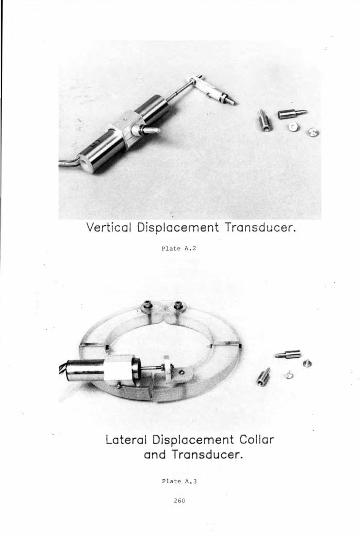
Vertical Displacement Transducer.

Plate A.2

Lateral Displacement Collar and Transducer.

Plate A.3

260

. .

/ r

Deformation Measuring System.

Plate A.4

26 1

A.8 The Testing Prograrnne.

The vertical stress consisted of a 32 KN/m2

constant value

'dead load' , onto which the dynamic pulse was superJ..rnr:osed. It was

appreciated that this value of 'dead load' ..as high in relation to the

likely overburden pressure to be expected in a pavanent but it was

selected in order to ensure that the, top end platen remains in contact

with the specimen during testing. The tyre. pressure of the oeflectogr­

aph rear wheel is arout 690 KN/m2 • The total vertical pressure of

1380 KN/m2 , pressure of twin rear wheels, was applied to· the sample

at different static confining pressures of lOO, 200, 300 KN/m2 :. The

speed of the Deflectograph is arout 2.5 Km/hr. The width of the Defle-

ctograph tyre is arout 230 rrm. Assuming, 45 degrees of load spread,

the frequency of the vertical stress was calculated as follOINS:

[o.5a !o.5a

t = S/V, f = 1/(2 t) I

H = Sample Thickness; 100 to 140 rrm,

V = 2.5 Km/hr = 694.44 rrm/sec,

S = (240 + H) rrm,

Range of f = 0.32 to 0.28 Hz.

Therefore a frequency of 0.3 Hz was the vertical stress pulse used for

all tests. The testing was carried out1\8 °c. The rrodulus was calcu­

lated after arout 300 cycles. After alx:iut 250 cycles the curve of the

plot of deformation against time tended to becane flat. This is proba-

bly due to the fact that the samples were already cx:mpacted by the

!lOVing traffic on the roads and the initial changes reflected 'bedding

in' of the testing system and particularly 'bedding in' of the sample

ends.

The elastic rrodulus of the bituminous samples was between 2.5

to 5 x 109 N/~. The elastic rrodulus increased with the increase

in confining pressure.

262