Embed Size (px)
Citation preview

NASA
Contractor Report 191057
Advanced Rotorcraft Transmission
(ART) Program- Final Report
Army Research Laboratory
Contractor Report ARL-CR-14
//v -3_
Gregory F. Heath
McDonnell Douglas Helicopter Company
Mesa, Arizona
and
Robert B. Bossier, Jr.
Lucas Western, Incorporated
Applied Technology Division
City of Industry, California
January1993
Prepared forLewis Research Center
Under Contract NAS3-25454
_0,0
N tO 0! P,-
rn U _'_O" CZ :_ 0
I
0
c_ +J¢3,,_ ¢3.Lu .-,, O
UZ Z ,-
<[O ,--::" ,--* (I)
:E CLm
O_ _" Ir-I I-... p-I u. LL _-
_3E C
t_
f_
U.S. ARMY
NASANational Aeronautics andSpace Administration RE,OF.ARCH LABORATORY
https://ntrs.nasa.gov/search.jsp?R=19930013277 2018-07-26T19:03:11+00:00Z


PHASE I
FINAL REPORT
ADVANCED ROTORCRAFT TRANSMISSION PROGRAM
(ART)
Prepared For:
U,S. Army Propulsion Directorate
National Aeronautics and Space AdministrationLewis Research Center
Cleveland, Ohio 44135

CONTENTS
I* SUMMARY ............................................................................................ 1
II. INTRODUCTION ......................................................................................................................................... 3
II.A ART Phase I Transmission Preliminary Design and Component Development Task
Descriptions .................................................................................................. , ....................................... 3
II.B Tooth Scoring Tests, Single Tooth Bending Fatigue Tests, and Charpy Impact
Energy Tests - Gear Materials ............................................................................................................ 7
II.C Fracture Toughness Tests - Gear and Housing Materials .............................................................. 8
II.D Tensile Tests - Housing Materials ...................................................................................................... 8
III. PRELIMINARY DESIGN ........................................................................................................................ 10
III.A Introduction ......................................................................................................................................... 10
III.B ART Team Drive Systems Engineering Methodology ................................................................... 10
III.C Weight Design Information ............................................................................................................... 12
II1.C.1
III.C.2
II1.C.3
Weight Prediction Methodology ......................................................................................... 13
Transmission Weight Results .............................................................................................. 13
Weight Comparison Summary ........................................................................................... 13
III.D Reliability Evaluation ................................................................. 14
III.D.1
III.D.2
III.D.3
Reliability Introduction .......................................... 15
Reliability Evaluation Procedure and Results ..................................................................... 15
Reliability Evaluation Discussions and Conclusions...., ..................................................... 16
III.E Noise Prediction .................................................................... ....,:.................................... 16
III.E.1
III.E.2
Estimation of Transmission Noise Levels ........................................................................... 16
Noise Prediction Results ............................................. • ....................................................... 17
III.F Summaryof Results ........................................................................................................................... 17
III.G Conclusions ......................................................................................................... ...._.................. 18
IV. ART TRANSMISSION DESIGN AND ANALYSIS ....................................................................... 19
IV.A
IV.B
IV.C
IV.D
Transmission Configuration ............................................................................................................. 19
Gear Analysis ........................................... :.................................................................................... 39
Bearing Analysis ................................................................................................................................ 41
Gear Shaft Structural Analysis ......................................................................................................... 42
lCR.N?t0N113,! R¢l_ PRE'I_DING P/_E BLANK NOT RLMED

CONTENTS (Continued)
IV.E Mass Properties Analysis ................................................................................................................. 45
IV.E.1
IV.E.2
IV.E.3
IV.E.4
Introduction ......................................................................................................................... 45
Summary Profile and Outline of Art Weight Goals ............................................................. 45
Volumetric Weight Analysis ................................................................................................ 46Conclusions ........................................................................................................................ 47
IV.F Supportability ..................... ................................................................................................................ 55
IV.F.1
IV.F.2
IV.F.3
IV.F.4
Abstract ............................................................................................................................... 55
Introduction ......................................................................................................................... 55
Reliability .............................................................................................................................. 56
Maintainability ...................................................................................................................... 67
IV.F.5 Supportability Discussion 75
IV.G Acoustic Assessment ........................................................................................................................ 77
IV.G.1
IV.G.2
IV.G.3
IVoG.4
IV.G.5
IV.G.6
IV.G.7
IV.G.8
IV.G.9
IV.G.10
IV.G.11
Summary ............................................................................................................................. 77Introduction ......................................................................................................................... 77
Methodology ....................................................................................................................... 79
Description of the AH-64 Apache Transmission ................................................................ 84
Application of Methodology to the AH-64 Transmission ................................................... 85
Experimental Program ........................................................................................................ 95
Comparison Between Analysis and Experiment ................................................................ 96
Description of the MDHC Advanced Rotorcraft Transmission ........................................ 102
Application of Methodology to ART ................................................................................. 105Discussion of Results ........................................................................................................ 110
Summary of Results .......................................................................................................... 111
V. MISSION EFFECTIVENESS ..............................................................................................................113
V.A Mission Analysis ............................................................................................................................... 113
V.B Approach .......................................................................................................................................... 114V.C Threats .......................................................................................................................................... 114
iv

CONTENTS (Continued)
VI.
PaQe
V.D Engagement Model .......................................................................................................................... 114
V,E Results and Conclusions ................................................................................................................ 116
Results ............................................................................................................................... 116
Conclusions ....................................................................................................................... 119
V.F Reliability .......................................................................................................................................... 119
V.F.1
V.F.2
FAAV Mission Reliability .................................................................................................... 119
FAAV System Reliability .................................................................................................... 121
V.G Life Cycle Costs ................................................................................................................................ 121
V.G.1
V.G.2
V.G.3
V.G.4
Methodology ..................................................................................................................... 121
System Description ........................................................................................................... 122
Acquisition Cost Estimates (Ground Rules and Assumptions) ....................................... 122
Operating and Support Cost Estimate ............................................................................. 126
V.H Conclusions ...................................................................................................................................... 128
MATERIAL CHARACTERIZATION TESTS .................................................................................129
VI.A Introduction ....................................................................................................................................... 129
VI.B Test Programs ................................................................................................................................... 130
VI.B.1
VI.B.2
VI.B.3
VI.B.4
VI.B.5
VI.B.6
Gear Tooth Scoring Tests .................................................................................................. 130
Single Tooth Bending Fatigue Tests ................................................................................. 140
Charpy Impact Energy Tests - Gear Materials .................................................................. 156
Fracture Toughness Tests ................................................................................................. 161
Tensile Tests - Housing Materials ...................................................................................... 172
Face Gear Capacity Tests .................................................................................................. 181
VII. SUMMARY OF RESULTS - CONCLUDING REMARKS ........................................................184
V

CONTENTS (Continued)
APPENDICES
A
B1
B2
REFERENCES
POSITIVE ENGAGEMENT CLUTCH ANALYSIS ............................................................................ 186
LIFE AND RELIABILITY FOR SYSTEMS USING WEIBULL
DISTRIBUTIONS ............................................................................................................................... 195
FAILURE MODES EFFECTS AND CRITICALITY ANALYSIS (FMECA) ...................................... 197
................................................................................................................................................ 202
vi
1
8
9
10
11
12
13
14
15
16
17
18
19
2O
FIGURES
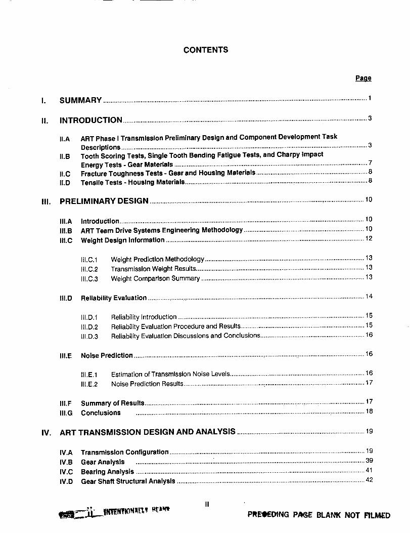
Three-Stage Split Torque Transmission Preliminary Design .............................................................. 11
Four-Stage Single-Planetary ART Candidate Configuration ............................................................... 12
ART Transmission Configuration ......................................................................................................... 20
ART Positive Engagement Clutch ........................................................................................................ 20
ART Gear and Shaft Schematic ........................................................................................................... 22
ART Plan View ....................................................................................................................................... 23
ART Input Stage.................................................................................................................................... 28
ART Second Stage and Planetary Third Stage ................................................................................... 28
ART Face-Up Face Gears/Lubrication Pump Drives.......................................................................... 29
ART Combining Gear/NOTAR Drive and Planetary Stage ................................................................. 31
ART Baseline Planetary Design............................................................................................................ 32
ART Aft View of Housing ...................................................................................................................... 33
ART Plan View of Housing .................................................................................................................... 34
ART Profile View of Housing ................................................................................................................ 34
ART Transmission Case, Tri-Metric View Looking Down .................................................................... 35
ART Transmission Case, Tri-Metric View Looking Up ......................................................................... 35
Lubrication System Schematic ............................................................................................................ 36
Nominal Cost Distribution of a Typical DoE) Program ........................................................................ 55
Reasons for Transmission Removals................................................................................................... 58
ART (top) Vs. Apache Miscellaneous Failure Rates............................................................................ 60
vii

21
22
23
24
25
26
27
28
29
30
31
32
33
34
35
36
37
38
39
4O
41
FIGURES (Continued)
S-NCurvefor AGMA and NASA .......................................................................................................... 62
Effect of Load-Life Factor on Life Equivalent Power ........................................................................... 64
ART Reliability Vs. Hours ...................................................................................................................... 67
Most Commonly Found Discrepancies ............................................................................................... 68
Causes of Contamination ..................................................................................................................... 69
Causes of Leaking ................................................................................................................................ 71
Parts with Corrosion ............................................................................................................................. 73
Transmission Noise Prediction Scheme .............................................................................................. 80
The AH-64 Apache Helicopter Transmission (cutaway view) ............................................................. 84
The AH-64 Apache Helicopter Transmission Outer Casing ................................................................ 85
LWI FE Model of the AH-64 Apache Helicopter Transmission ........................................................... 86
Reduced FE Model of the Apache Helicopter Transmission Casing ................................................. 87
Finite Element Model of the Apache Transmission Gears .................................................................. 88
Finite Element Model of the Apache Helicopter Transmission ........................................................... 91
Typical Stress Contour Plot from a Gravity Loading Analysis ............................................................ 91
Boundary Element Model of the AH-64 Apache Helicopter Transmission ........................................ 93
SEA Model of the AH-64 Apache Helicopter Transmission ................................................................ 94
Measured Sound Power Spectrum of the Apache Helicopter Transmission .................................... 95
Measured Noise Levels in the Cockpit of the Apache Helicopter ...................................................... 96
Measured vs. BEMAP-Predicted Sound Power Levels ....................................................................... 98
Measured vs. SEA-Predicted Sound Power Levels ............................................................................ 99
viii
42
43
44
45
46
47
48
49
5O
51
52
53
54
55
56
57
58
59
6O
61
62
FIGURES (Continued)
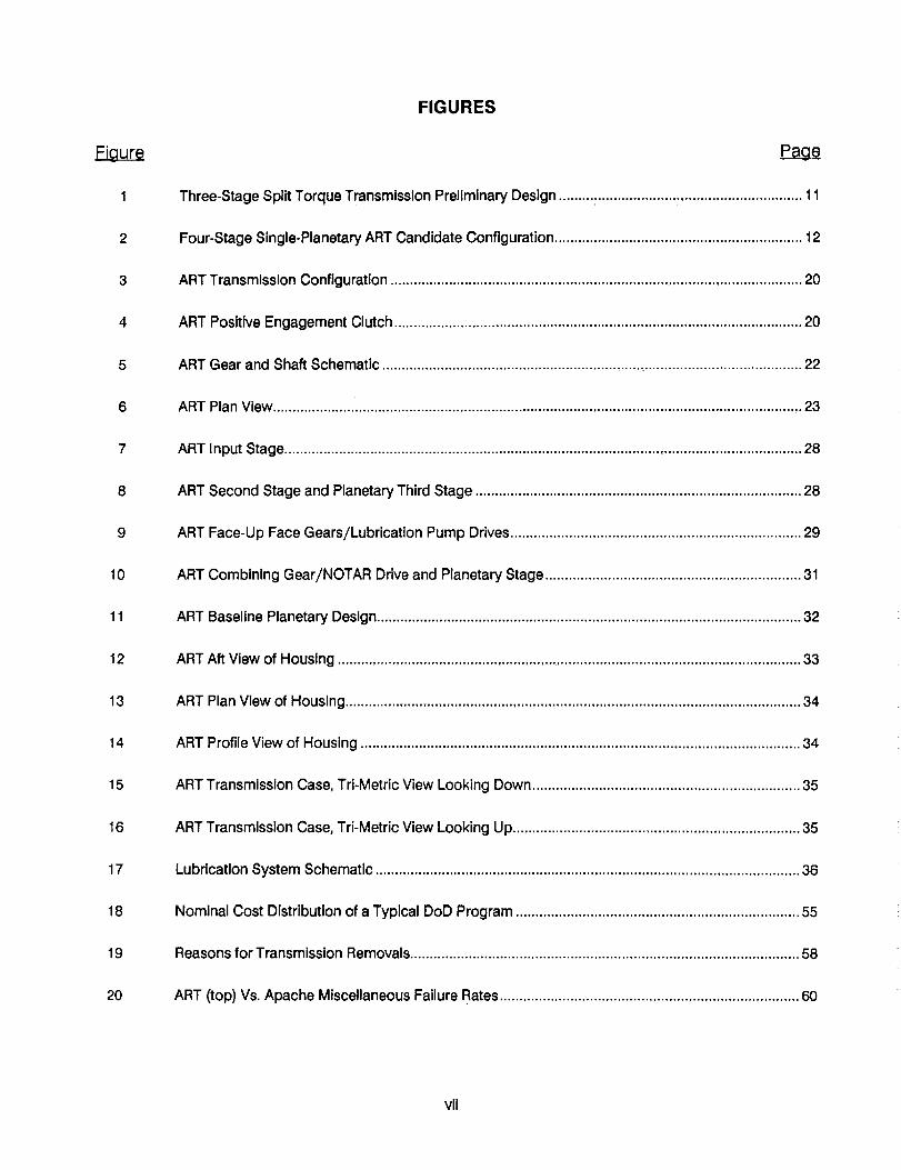
Measured vs. Combined (BEM and SEA) Predicted Sound Power Levels ........................................ 99
Surface Noise Contour on Transmission Houslng at Planetary Gear Mesh (665 Hz) ..................... 101
Effects of Structural Damping on Predicted Gearbox Noise Levels ................................................ 101
ART Gear Arrangement ...................................................................................................................... 102
ART Outer Casing ............................................................................................................................... 103
ART Transmission Noise Goal from Apache Transmission Noise Trend Data ................................ 104
FEM of ART Internal Components ..................................................................................................... 105
ART Top Cover ................................................................................................................................... 106
ART Intermediate Caslng ................................................................................................................... 106
FEM of ART Lower Casing ................................................................................................................. 107
Complete FEM of ART........................................................................................................................ 107
Stress Contour Plot from Static Gravity Loading .............................................................................. 108
ART Boundary Element Model ........................................................................................................... 109
Speed Power Polar Comparison Apache FAAV................................................................................ 117
FAAV Configurations .......................................................................................................................... 1t 8
Trend in Military Helicopter System Reliability.................................................................................. 120
NASA-Lewis Gear Fatigue Test Fixture ............................................................................................. 135
MDHC Tooth Scoring Test Fixture..................................................................................................... 135
Scoring Test Fixture Calibration Curve .............................................................................................. 136
Scoring Test Flash Temperatures ...................................................................................................... 138
Flash Temperature vs. Probability of Scoring ................................................................................... 138
_x

63
64
65
66
67
68
69
70
71
72
73
74
75
76
77
78
79
80
81
82
Detail Views of Test Gears .................................................................................................................. 143
Test Tooth and Load Anvil ................................................................................................................. 144
Single Tooth Bending Fatigue Test Fixture ....................................................................................... 144
Strain Gage and Crack Wire Placement ............................................................................................ 145
Best Fit S-N Curve of Single Tooth Bending Fatigue Tests, Material: M50NIL ............................... 152
Best Fit S-N Curve of Single Tooth Bending Fatigue Test, Material: X53 ....................................... 152
Best Fit S-N Curve of Single Tooth Bending Fatigue Tests, Material: CBS 600 ............................. 153
Best Fit S-N Curve of Single Tooth Bending Fatigue Tests, Material: 9310 .................................... 153
Best Fit S-N Curve of Single Tooth Bending Fatigue Tests, Material: Maraglng 300 ..................... 154
Comparison of Best Fit S-N Curves for Five Gear Materials ............................................................ 155
Charpy V Impact Specimen ............................................................................................................... 158
Tension Test Specimen ...................................................................................................................... 159
Fracture Toughness (Klc) Specimen, B= 1.00"................................................................................ 165
K1c" Load Versus Displacement ....................................................................................................... 172
Tensile Specimen (Plain Cylindrical Ends) ........................................................................................ 174
Tensile Specimen (Button Head Ends) ............................................................................................. 174
WE43 Stress-Time Curve ................................................................................................................... 179
WE43 Stress-Strain Curve .................................................................................................................. 179
Gears installed in Test Stand ............................................................................................................. 182
NASA Spiral Bevel Gear Rig............................................................................................................... 183

83
84
85
FIGURES (Continued)
Section Integrated System Used to Calculate Polar Mass Moment of Inertia and CentrifugalForce Moment of Pawl ....................................................................................................................... 187
Pawl Behavior vs. Differential Input to Output Speed ....................................................................... 192
ART Reliability Block Diagrams .......................................................................................................... 200
xl

Table
6
8
9
10
11
12
13
14
15
16
17
18
19
20
21
LIST OF TABLES
GEAR MATERIALS - RELATIVE RANKINGS .......................................................................................... 8
HOUSING MATERIALS - RELATIVE RANKINGS .................................................................................. 9
PRELIMINARY DESIGN BASELINES AND ALLOWABLES ................................................................. 11
CANDIDATE ART CONFIGURATION RATING TABLE ........................................................................ 18
SHAFT SPEED/LOAD TABLE .............................................................................................................. 22
GEAR SPEED/LOAD TABLE ............................................................................................................... 23
ART DESIGN PARTS LIST.................................................................................................................... 24
PLANETARY COMPARISON TABLE ................................................................................................... 31
BASELINE PLANETARY VERSUS HIGH CONTACT RATIO PLANETARY DESIGN .......................... 32
SUMMARY OF GEAR STRESS ANALYSIS .......................................................................................... 40
SUMMARY OF ART GEAR DESIGN LIFE VALUES ............................................................................. 40
ART BEARING DESIGN AND CALCULATED LIFE VALUES ............................................................... 41
SUMMARY OF GEAR SHAFT STRESS ANALYSIS ............................................................................. 44
ART WEIGHT PROFILE ........................................................................................................................ 45
ART TRANSMISSION ASS EMBLY PARAMETRIC WEIGHT CHECK .................................................. 46
ART VOLUMETRIC WEIGHT SUM MARY............................................................................................. 47
ART GEARBOX DETAIL WEIGHT ........................................................................................................ 48
MISCELLANEOUS FAILURES AND FAILURE RATES ........................................................................ 60
LIFETIME POWER PROFILES ............................................................................................................. 64
RELIABILITY PARAMETERS FOR CALCULATION OF ART MTBR .................................................... 66
COMPARISON BETWEEN MEASURED AND PREDICTED VIBRATION LEVELS ............................. 97
xll

Table
22
23
24
25
26
27
28
29
3O
31
32
33
34
35
36
37
38
39
40
41
42
LIST OF TABLES
TRANSMISSION NOISE PREDICTION VALIDATION ........................................................................ 100
ESTIMATED NOISE LEVEL FOR BASELINE TRANSMISSION ........................................................ 104
LINEAR PROFILE MODIFICATION DATA FOR GEAR TEETH ......................................................... 109
TRANSMISSION NOISE PREDICTION ERROR CORRECTION ....................................................... 110
ART NOISE PREDICTIONS ................................................................................................................ 111
AIRCRAFT CONFIGURATIONS AND WEAPONS LOADS ................................................................ 115
TOTAL R&D ......................................................................................................................................... 124
TRANSMISSION R&D ESTIMATE ...................................................................................................... 124
INVESTMENT ...................................................................................................................................... 125
ART RECURRING PRODUCTION COST ........................................................................................... 125
O&S COST .......................................................................................................................................... 127
DOC ................................ _................................................................................................................... 127
WEIGHT/LIFE CYCLE COST COMPARISON ................................................................................... 128
MATERIAL CERTIFICATES ................................................................................................................ 132
CHEMICAL COMPOSITIONS ............................................................................................................ 132
SPECIFIC HEAT TREATMENTS ......................................................................................................... 133
SUMMARY OF SCORING TEST DATA .............................................................................................. 137
FLASH TEMPERATURES (OF), SCORING RISK ............................................................................... 139
TEST SPECIMEN MATERIALS AND QUANTITIES ........................................................................... 139
MATERIAL CERTIFICATES ................................................................................................................ 141
CHEMICAL COMPOSITION ............................................................................................................... 141
xiii

Table
43
44
45
46
47
48
49
50
51
52
53
54
55
56
57
58
59
60
61
62
LIST OF TABLES
HEAT TREATMENTS, CORE/CASE HARDNESS AND CASE DEPTH AT PITCH LINE .................. 142
M50NIL SINGLE TOOTH BENDING FATIGUE TEST DATA ............................................................. 147
X53 SINGLE TOOTH BENDING FATIGUE TEST DATA .................................................................... 148
CBS 600 SINGLE TOOTH BENDING FATIGUE TEST DATA............................................................ 149
9310 SINGLE TOOTH BENDING FATIGUE TEST DATA .................................................................. 150
M300 SINGLE TOOTH BENDING FATIGUE TEST DATA ................................................................ 151
STATISTICAL EVALUATION OF TEST DATA .................................................................................... 154
MATERIAL CERTIFICATES ................................................................................................................ 156
CHEMICAL COMPOSITION ............................................................................................................... 157
SPECIMEN SIZE, SPECIMEN CONFIGURATION, AND SPECIMEN ORIENTATION ..................... 157
CORE HEAT TREATMENTS AND REQUIRED MECHANICAL PROPERTIES AT
ROOM TEMPERATURE ...................................................................................................................... 158
SUMMARY - CHARPY V IMPACT ENERGY TEST RESULTS ........................................................... 160
MATERIAL CERTIFICATES ................................................................................................................ 162
CHEMICAL COMPOSITION ............................................................................................................... 163
SPECIMEN SIZE, SPECIMEN CONFIGURATION, AND SPECIMEN ORIENTATION ..................... 164
HEAT TREATMENTS AND HARDNESS ............................................................................................ 166
TENSILE PROPERTIES ................................................... :.................................................................. 167
FRACTURE TOUGHNESS TEST RESULTS ...................................................................................... 168
Klc DATA SUMMARY ........................................................................................................................ 170
MATERIAL CERTIFICATES ................................................................................................................ 173
xiv

63
64
65
66
67
68
69
7O
71
72
73
74
LIST OF TABLES
CHEMICAL COMPOSITION ............................................................................................................... 173
TEST DATA OF WE43 ........................................................................................................................ 176
TEST DATA OF ZE41A ....................................................................................................................... 177
TEST DATA OF C355T7 ..................................................................................................................... 178
HEAT TREATMENTS AND HARDNESS ............................................................................................ 178
TENSILE PROPERTIES (MATERIAL: WE43) .................................................................................... 180
TENSILE PROPERTIES (MATERIAL: ZE41A) ................................................................................... 180
TENSILE PROPERTIES (MATERIAL: C355T7) ................................................................................. 180
TENSILE TEST RESULTS SUMMARY ............................................................................................... 181
PAWL POLAR MASS MOMENT OF INERTIA, J ................................................................................ 188
PAWL CLOCKWISE AND COUNTERCLOCKWISE SECTION MOMENTS ...................................... 189
FAILURE MODES, EFFECTS AND CRITICALITY ANALYSIS ........................................................... 198
XV

This page Is Intentionally left blank.
xvl

I. SUMMARY
TheTeamofMcDonnellDouglas Helicopter Company (MDHC) and teammate/subcontractor Lucas Western,
Inc. (LWI) have developed a concept which meets or exceeds all of the goals of the Advanced RotorcraftTransmission (ART) Program. The total calculated weight of the transmission assembly Is 40 percent below the
SOA transmission weight compared to the goal of 25 percent. The noise reduction goal of 10 dB is essentiallymet with a predicted reduction of 9.6 dB. Reliability of the ART exceeds the 5000-hour MTBR goal by 1270hours.
This report summarizes design work performed by MDHC and LWI, within the Army/NASA ART Program. Itdescribes the ART Program Task IV detail design of a 5000-horsepower transmlssion for an early 21st centuryFuture Attack Air Vehicle (FAAV) weighing about 16,000 pounds. Government goals set for the program were todefine technology and detail design the ART to meet, as a minimum, a weight reduction of 25 percent, aninternal noise reduction of 10 dB plus a Mean Time Between Removal (MTBR) of 5000 hours compared to a
state-of-the-art (SOA) baseline transmission.
A novel three-stage ART transmission concept was developed to meet the requirements. It features a torquesplitting configuration using face gears. On each side of the transmission, a single input spur gear drives twoface gears simultaneously. This splitsthe torque into two nearly equal load paths, each face gear shafttransmitting reduced torque untila recombination occurs at a second stage collector gear. The separate loadpaths allow significant downsizing of first and second stage components beyond the high-volume geometriesthat would have been required to carry full load. A high contact ratio third stage planetary with a flexured ringgear also yields reduced weight and noise levels for the transmission. Optimized gear web design and selectionof advanced housing materials represent other technology Improvements. Overrunning positive engagement
clutches on the Input shafts and an advanced lubrication system further advance the weight and reliabilityadvantages of the configuration. System design methods such as an optimized combination of gear ratios,
computerized reliability methodology interactive with gear and bearing design allowables, and partiallyoverlapping second and third stages were also used to reduce weight. The total calculated weight of the
transmission assembly is 815 Ib, 40 percent below the SOA transmission weight. The predicted source noiselevel for the ART is 98.3 dB, which is 9.6 dB below the 107.9 dB SOA noise level for the upscaled baseline 5000-horsepower Apache transmission. The Army/NASA goal for noise reduction was 97.9 dB, 10 dB below the107.9 dB SOA noise level. Reliability of the ART is 6270 hours MTBR, 1270 hours above the 5000 hour goal.MDHC mission analysis shows that the above FAAV with ART produces a 17 to 22 percent Improvement in theloss exchange ratio compared to the baseline FAAV. In addition, the improvement in mission reliabilitytranslates to a 22 percent Increase in MTBF, while system reliability Increased 25.5 percent in MTBF. Also,transmission direct operating cost decreased above 33 percent. The three stage, single planetary split torquedesign offers substantial improvement over conventional 5000 horsepower design practice.
The mission performance improvements and cost savings resulting from the ART transmission designachievements described above are substantial. Installing the 5000 HP ART transmission in a 16,000-1b FAAV,rather than a 5000 HP state-of-the-art baseline transmission, would result in a 17 to 22 percent Improvement Inloss-exchange ratio during combat, a 12 percent Improvement inthe ability to sustaln a given level of combat
operations and a 22 percent improvement in MTBF. Use of the ART would also result in a transmissionacqulsition cost savings of 23 percent or $165K, per unit. An average transmission direct operating cost savingsof 33 percent, or $24 per flight hour, would also be realized.
PREQEDING PAGE BLANK NOT FILMED

Toothscoringtests, single tooth bending tests, Charpy Impact energy tests and compact tension fracturetoughness tests were performed with five high temperature gear materials. Also, compact tension fracturetoughness tests and tensile strength tests were performed with three advanced housing materials.Recommendations for additional detail design, analysis, fabrication, and testing are made for follow-on work to
the ART Program Phase I work described in this report.

II. INTRODUCTION
TheU.S. Army, in cooperation with the National Aeronautics and Space Administration, initiated the AdvancedRotorcraft Transmission (ART) Program to develop and demonstrate improvements in state-of-the-art (SOA)rotorcraft transmissions. The main focus of the ART Program is to develop key emerging material, component,
subsystem and manufacturing technologies along the same pathways traditionally followed in new enginedevelopment. Engines typically are tested and perfected over a period of years, long before transmissiondesign and development begins for aircraft application.
The McDonnell Douglas Helicopter Company (MDHC) and teammate, Lucas Western, Inc. (LWI), ART is sizedfor the Future Attack Air Vehicle (FAAV) of the early 21st century. The FAAV is visualized as a rotorcraft having
extremely enhanced maneuverability at nap-of-the-earth altitudes along with improved performance In all flightregimes. FAAV requirements and vehicle concepts were evaluated early in the program to define a rotorcraft Inthe 10,000 to 20,000 pound gross weight range using an ART rated in the 5000 horsepower class. A 5000horsepower version of the AH-64A Apache helicopter was used as the FAAV baseline aircraft, and an Apachemain transmission parametrically upscaled to 5000 HP served as the baseline $OA transmission for comparisonwith the ART.
II.A ART PHASE I TRANSMISSION PRELIMINARY DESIGN AND COMPONENT DEVELOPMENT TASK
DESCRIPTIONS
Task 1 - SQIQ_tiqn Qf Evaluation Procedures and AssumDtions
Select the procedures and ground rule assumptions for conducting tradeoff studies for the design of an
advanced technology transmission for an FAAV. These procedures and ground rules shall be used in
conducting Task 2 and Task 3.
Task 2 - Transmission Confiquration and OI3eration Evaluation
Prepare the preliminary designs for and evaluate advanced technology transmissions applicable to the FAAV.
The goals are to reduce transmission weight by 25 percent, reduce source noise in the transmission by 10dB,and Increase the MTBR to 5,000 hours.
Recommend a transmission configuration and present the study results to the U.S. Army Propulsion Directorate
Project Manager for approval.
Task 3 - System performance Evaluation
Conduct a mlssion analysis to determine the effects on performance of the selected FAAV.

Task4- Detail Desiqn and Ana!vsls of ART Components for Test
Based on the transmission configuration approved in Task 2, proceed with the detailed design and analysis of
all components and subsystems. The design layout and analysis shall be used to determine estimated system
weight (including lubrication and cooling requirements), probable noise levels, theoretical component life, and
assembly integrity under loading and operating conditions expected in the transmission.
Identify the crucial components and subsystems for test.
Task 5 - Devsl0pment of Component and Subsystem Test Plan
Develop a detailed component test plan based on the results of Task 4. The test plan shall provide rationale for
the types of tests to be conducted and data to be acquired from the tests. Submit the test plan to the U.S. Army
PM for approval.
Task 6 - Preparation of Component Test Rig
Provide or make arrangements for component test rigs.
Task 7 - Fabrication of Component Test Articles
Fabricate the number of test articles of components or subsystems identified inTask 4 for verification testing to
complete the plan developed inTask 5.
Task 8 - Performance of Component Verification Test and Individual Assessment
Perform the component tests called for inthe approved test plan submitted under Task 5.
Task 9 - RePOrt Requirements
Submit a written Final Report covering all the effort conducted.
Art Program Phase I was started in 1988 and is now complete. It was structured for performance oftransmission preliminary design and component development. ART Program Phase II is scheduled as ademonstrator phase, during which an ART transmission or individual subsystems will be detail designed,fabricated and tested. The main purpose of the Phase I design and analysis efforts has been to attain the U.S.
Army/NASA goals for the transmission weight, noise and reliability. Specifically, the Army/NASA goals were todesign an ART that, relative to the SOA baseline transmission, achieved at least a 25% weight reduction, a 10 dBreduction in source noise and a mean-time-between-removal (MTBR) life of 5000 hours. Testing performed to
substantiate the transmission component and subsystem concepts developed and materials utilized indicated
the progress attained in meeting the goals and validating new design concepts.

This report covers the work performed by MDHC and teammate/subcontractor LWl under Phase 1 of the
Advanced Rotorcraft Transmission (ART) Program. The efforts concentrated on high gain and comparatively
high risk developments that were evaluated systematically to solve problems prior to full scale development.
Advanced and innovative technology has been identified in the MDHC/LWl candidate for further development
and testing as part of the ART program.
Section III, Preliminary Design, covers Tasks 1 and 2. To satisfy Task 1, Selection of Evaluation Procedures andAssumptions, a letter was written to specify the procedures and ground rules to be used in carrying out thedeslgn processes. We identified the FAAV as an upscaled AH-64A Apache, having two engines driving a mainrotor, anti-torque fan and accessories through a main transmisslon. The input shaft speed from each engine Is20,952 rpm, and the main rotor speed is 289 rpm. The dual engine rated power for the transmission baseline is
5000 horsepower, and the maximum continuous single-engine power is 2500 horsepower. The one-engine-inoperative (OEI) power requirement for emergency single engine flight is 3000 horsepower. All gears of thepreliminary design candidates were to be designed to carry the (::)Elhorsepower for thirty minutes or more. Inaddition, all gears and bearings were to be designed without exceeding American Gear ManufacturersAssociation (AGMA) and Anti-Friction Bearing Manufacturers Association (AFBMA) stress allowables whileachieving at least the minimum component lives required to attain a 5000 hour system MTBR.
In performing Task 2, Transmission Configuration and Operation Evaluation, candidate transmission
configurations were defined to meet the design requirements of the FAAV and the allowables selected in Task I.
Load and speed carrying capabilities, preliminary bearing and gear lives, and preliminary weight and noise
design considerations were analyzed and sketches of the transmission concepts under consideration were
produced. Weight, reliability and noise analysis methods were then applied to the designs to evaluate these key
operational parameters. Results of the analysis work are presented in this report. A final downselection was
made between the two most promising configurations using a matrix evaluation process. This evaluation
procedure rated the candidate configurations in terms of apparent progress made in meeting Army/NASA goals
in addition to secondary factors such as direct operating cost and risk assessment. The goal factors were given
a weighted priority of Importance of 0.5, 0.3 and 0.2 respectively for the evaluation. Direct operating cost and
risk assessment factors were evaluated for use in the event of a near-tie between the configurations scored.
The ART transmission chosen through the above downselection process was a novel three stage, single
planetary, split torque concept using face gears. A spur gear pinion located on each input drive shaft drives two
face gears simultaneously, providing a split of the torque at the first stage. The face gears rotate In the same
direction, and the torque Is recombined on a large bull gear above through two second stage spur pinions. The
bull gear drives a high contact ratio planetary, which in turn drives the main rotor. Key subsystems of the
transmission Include two positive engagement input clutches and an advanced lubrication system.
Section iV, ART Transmission Design, covers Task 4, Detail Design and Analysis of ART Components for Test.
The three stage split torque configuration selected in Task 2 was further developed and refined during Task 4.
The design effort focused on attaining the U.S. Army/NASA weight, noise and reliability goals describedpreviously.
The three stage split torque configuration, first sized in Task 2, provided a low weight starting point for Task 4.During Task 4, weight reduction was enhanced when the combination of gear reduction ratios used for the three
stages of the split torque transmission was optimized to achieve a minimum weight for the configuration. Thisminimum weight assessment was based on iterative computer runs performed with a parametric weights

analysisprogram which considered the gear and bearing arrangements as well as component materials andgeometries. As in the design processes for earlier downselectlon, AGMA and AFBMA stress analyses and lifecalculations were performed in assurlng an ART with a system life of 5000 hours MTBR and OEI operatlonalcapability. Additional weight reduction was achieved during the detail design of individualtransmission
components.
Stress analyses performed on the transmission included modeling the gear webs, rims, and shafts of the threeindividual stages to analyze deflections. Deflections of the two first stage face gears were equalized andminimized through a design-interactive process. Equallzed stiffness, In addition to first and second stage toothphasing and a flexible input pinion support, assured near-equal torque splitting to the gears. Planetary carderdeflections were analyzed during the design process to achieve good strength-to-weight design. Deflections ofthe cantilevered planetary rlng gear were also determined to assure controlled radial motion of the six plnlons
and to provide suitable fatigue life.
As the ART design neared completion, a NASTRAN finite element model of the transmission was produced toobtain output vibration levels of the transmission during operation. This information was then used for theacoustic calculations, which were accomplished by two distinctly different procedures. A deterministicapproach, based on the boundary element method, was used for determining the case-radiated noise at thelowest gear mesh frequencies. Given the demand for large amounts of computer memory for the boundaryelement method, it was found practical to supplement this method with a stochastic approach, based on
statistical energy analysis (SEA), for evaluation of the higher frequencies. SEA could not be used exclusivelybecause of its limited precision at the lower frequencies where the boundary element method performed best.The overall noise prediction methodology, which incorporates a combination of both approaches, wasimplemented to evaluate the noise emissions of a transmission currently used in the AH-64 Apache helicopter.Vibration and noise levels from the Apache transmission models were correlated with actual test data. This test-correlated methodology was then used in developing and analyzing ART. The methodology Is intended toallow for "design-to-noise" capability.
Noise reduction methods employed during the design process included minimizing gear web, rim and shaftdeflections. Also, a high contact ratio (HCR) third stage planetary having properly phased gear tooth numbers,profile modification and a cantilevered ring gear was implemented. The ART split torque configuration, withdivided power paths, provides additional noise reduction. The transmission housing structural shape, webs andstiffenerswere also designed to minimize vibratory deflections.
The MDHC ART split torque configuration, design features and analysis methodologies are described in this
report. The completed transmission design was found to offer substantial progress towards the Army/NASAweight, noise and reliability goals, and can provide increased capabilities in a fielded aircraft.
Section V, Mission Effectiveness, covers Task 3, System Performance Evaluation. This section is segmentedinto three subsections:
• Mission Analysis
• Reliability
• Life-Cycle Costs
Mission Analysis is an assessment of lethality and survivability of the aircraft. As part of the ART program, an
evaluation of how the improved transmission impacted mission effectiveness was studied. Although the
changes being considered affected all areas of mission performance, past experience indicated that the most

demanding area would be a close-In, air-to-air engagement. Accordingly, the air-to-air engagement was the
focus of this analysis. The FAAV with ART produced a 17 to 22 percent increase in the loss-exchange ratio
compared to the baseline FAAV.
FAAV Reliability will be much improved over current generation aircraft. The amount of improvement is
estimated by trending previous and current design reliabilities. Assumlng the FAAV is a next-generation design,
the trend is to double reliability requirements every generation. This results in an FAAV system reliability of 18
hours with mission reliability increasing from 22 to 75 hours.
Life Cycle Costs (LCC) estimates were made for three configurations: baseline FAAV, ART improved FAAV, and
optimized FAAV with ART. This report contains the estimates and a discussion of the techniques and
assumptions used to make those estimates. The LCC estimate is reflective of the technological advances
(composites and integrated mission equipment) and operating conditions Inherent in designing and fielding an
aircraft in the next century. The estimated life cycle costs show significant savings for the FAAV with ART,
compared to the baseline FAAV.
Several key performance parameters of the FAAV were evaluated to determine the benefits that would be
derived from the performance characteristics of the selected ART configuration. These analyses focus on the
system, not just the transmission, and consider the synergism of the transmission performance on the FAAV as
a total system.
Section VI, Material Characterization Tests, covers Task 5, Development of Component and Subsystem Test
Plan, Task 6, Preparation of Component Test Rig, Task 7, Fabrication of Component Test Articles, and Task 8,
Performance of Component Verification Test and Individual Assessment. Material testing was performed as
tabulated below, with the stated results.
II.B TOOTH SCORING TESTS, SINGLE TOOTH BENDING FATIGUE TESTS, AND CHARPY IMPACT
ENERGY TESTS - GEAR MATERIALS
These tests were performed on specimens fabricated from five different steels as tabulated.
Number of Tests
Material SDec. Tooth Scoring Tooth Bending
M50 MIL 6278 70 20 12
X53 Pyro. 6308 72 20 12
CBS 600 6255 6 12 12
AISI 9310 6265 96 24 12
300M 6514 6 12 12

II.C FRACTURE TOUGHNESS TESTS - GEAR AND HOUSING MATERIALS
These tests were performed on specimens fabricated from two magnesium alloys, one aluminum alloy, and two
steel alloys, as tabulated.
Material _ Heat Treatment NO. of Tests
WE43 4427 Solution Heat Treat 7
ZE41A 4439A Solution Heat Treat 7
C355T7 4215 Solution Heat Treat 6
M50 MIL 6278 Pseudocarburlzed/Hardened 6
X53 Pyro. 6308 Pseudocarburlzed/Hardened 7
II.D TENSILE TESTS - HOUSING MATERIALS
These tests Were performed on specimens fabricated from two magnesium alloys and one aluminum alloy, as
tabulated.
Material _ Heat Treotment No. of Tests
WE43 4427 Solution Heat Treat 24
ZE41A 4439A Solution Heat Treat 24
C355T7 4215 Solution Heat Treat 24
The relative rankings of the tested gear materials and housing materials, based on the test results, are shown in
Tables 1 and 2.
TABLE 1. GEAR MATERIALS - RELATIVE RANKINGS
Material
X53
M50Nil
CBS600
M300
AISI 9310
Single Tooth
Bending
1
3
2
4
5
Scoring
=
3
1
2
4
5
Fracture
Toughness
Charpy
Impact
8

TABLE 2. HOUSING MATERIALS - RELATIVE RANKINGS
Material
C355T7
WE43
ZE41A
Tensile Strength
1
2
3
Fracture Toughness
1
2
3
Section VII, Recommended Redesign and Retest, covers future activities recommended for the ART Program in
Phase II. During performance of ART Phase I, areas of the design and analysis Investigations with great
potential presented themselves. In addition to the ART prototype design and tests, other areas might be
profitably Investigated, such as two stage ART design and tests, positive engagement clutch tests, an expanded
face gear capacity test program with variations in material and manufacturing methods (including ground face
gears), acoustic modeling, and advanced materials investigation and implementation. Tested materials which
showed the highest performance during Phase I tests are recommended for high temperature tests and
subsystem integration tests.
9
III. PRELIMINARY DESIGN
IiI.A INTRODUCTION
The ART transmission selection and related methodology Is presented herein. Design baselines and allowableswere established in Task 1 for use in the preliminary design of candidate transmission configurations. Load and
speed carrying capabilities, preliminary bearing and gear lives, and preliminary weight and noise designconsiderations were analyzed for the two most promising configurations selected for Task 2. Two sketches
were produced, and weight, reliability and noise analysis methods were then applied to the designs to evaluatethese key operational parameters set forth within the original MDHC ART proposal. Results of the analysis workare presented in this report. Weighting factors and comparative analyses were applied to the results to yield a
unique ART design that promises to substantially advance the state of the rotorcraft transmission art.
III.B ART TEAM DRIVE SYSTEMS ENGINEERING METHODOLOGY
The transmission preliminary design analysis methodology used to develop the two candidate ART transmissionconfigurations began with establishing basic transmission requirements. Materials assumed for both the gearsand bearings used in this preliminary design phase were basic 9310 gear steel and 52100 bearing steel. Thenecessary power capacity, input and output speeds, loading and life allowables, and design envelope criteriawere determined. Table 3 lists the baselines and allowables used in preliminary design of the candidate
configurations. The next step in the design process was to select types of gearing, determine gear ratios, andsize the gears as a system to optimize weight and meet life requirements. The gear train designs conformed tothe established bending stress, hertz stress, pitch line velocity and flash temperature allowables of 9310 gearsteel.
Once gearing types and sizes were established, bearings were selected as per required type and basic C/Pload carrying capacity, based on allowables of 52100 bearing steel.
Computer programs were used to facilitate stress calculations for each gear type, geometry, and ratiocombination analyzed in preliminary design iterations. Existing programs used were the Gleason dimensionsheet program, the modified NASA CHOPR program, and AGMA-based spur and helical gear analysis
programs. The modified CHOPR program was used to calculate hertz stresses needed on each gear mesh toachieve a minimum overall 5000 hour MTBR for the gear trains of each candidate ART configuration.
Concurrent with the analyses described above, preliminary design sketches of the two candidate ART
transmission configurations were developed. Descriptions of the two configurations follow.
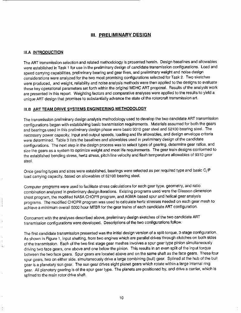
The first candidate transmission presented was the initialdesign version of a split-torque, 3-stage configuration.
As shown in Figure 1, input shafting, from two engines which are parallel drives through clutches on both sidesof the transmission. Each of the two first stage gear meshes involves a spur gear type pinion simultaneously
driving two face gears, one above and one below the pinion. This results in an even split of the input torquebetween the two face gears. Spur gears are located above and on the same shaft as the face gears. These four
spur gears, two on either side, simultaneously drive a large combining (bull) gear. Splined at the hub of the bullgear is a planetary sun gear. The sun gear drives eight planet gears which rotate within a large internal ringgear. All planetary gearing is of the spur gear type. The planets are positioned by, and drive a carrier, which is
splined to the main rotor drive shaft.
10

TABLE3. PRELIMINARY DESlGN BASELINES AND ALLOWABLES
DESIGN BASELINES
Engine Input Speed 20,950 RPM at engine output shaftMain Rotor RPM 289 RPM
Horsepower to Main Rotor 5000 HP
Overrunning clutches at transmission inputs from engine. Engines parallel or at 40-degree maximumincluded angle.
DESIGN ALLOWABLES
Gears Hertz Stress Allowables Bending Stress Allowables
Spiral Bevel Gears 220 ksi [1] 40 ksi [2]
Spur and Helical Gears 190 ksi [3] 60 ksi [3]
Pitch line velocity allowable = 22,500 ft/minute (for Rc 62 9310 steel, all gearing).Flash temperature less than 400°F [4].
Bearings: BIO lives all exceeded 10,000 hours for ART Preliminary Design. C/P ratings per allowables for52100 steel bearings [5,6].
Figure 1. Three-Stage Split Torque Transmission Preliminary Design
11

The second preliminary design candidate ART transmission was a 4-stage, single planetary configuration. Thistransmission, shown in Figure 2, runs the two engine inputs through two spiral bevel nose gearboxes. This firstspeed reduction ratio is about 2.22 to 1. The output shafting of each nose gearbox feeds into the maintransmission through a clutch and Inputs to a second spiral bevel gearset. Here a reduction of 2.45 to 1 occurs.Driven on the output shaft of this spiral bevel gear set is a herringbone gear. These double helical gears, one oneither side, simultaneously drive a large herringbone combining (bull) gear, and this gear ratio is 3.46 to 1.Located above the bull gear and splined to the same shaft Is a planetary sun gear. This gear drives six planetgears which rotate within a large internal ring gear. This final planetary ratio is 3.86 to 1. The planet gears areretained on a carrier which Is splined to the main rotor driveshaft. The carrier is driven by rotation of the planets
about the sun gear.
III.C WEIGHT DESIGN INFORMATION
The baseline helicopter is the Army AH-64 Apache upgraded to FAAV requirements. The industry weight trendfor a 5000 HP helicopter main transmission with an Apache main rotor speed of 289 RPM is 1792 Ib (installation
weight, includes main rotor driveshaft, static mast, and lubrication system) while the weight goal of the ART,with a 25 percent weight reduction is 1344 lb. The corresponding weights for the transmission assembly onlyare 1347 Ib for the industry weight trend and 1010 Ib for the ART goal with a 25-percent weight reduction.
.... >....l i
Figure 2. Four-Stage Single-Planetary ART Candidate Configuration
12

III.C.1 Weiqht Prediction Methodology
Weights of the Task 2 split torque transmission and the four stage single planetary transmission were estimated
by a parametric methodology described in Reference [7]. Using this method, the weight estimates for 39
gearboxes versus actual gearbox weights had a standard deviation of 9.3% with a correlation coefficient of .998.
The methodology was calibrated to the current Apache maln transmission weight, and the estimated weight was
above, but within 6% of the actual weight.
The weight prediction methodology is based on the three main components of transmissions (gears, bearings,
and housing), input and output drive train speeds and power capacities, and a sketch of the gear train.
Predicted weights were calculated based upon the above gearbox data.
III.C.2 Transmission Weiqht Results
The weight predictions used in down selecting the ART design were considered to be sufficiently accurate for
weight comparisons made during preliminary design. For the two candidate transmissions, the split torque
transmission and the four stage, single planetary transmission, weights are directly comparable to each other.
They do not include weights of the drive shaft(s), the static mast, and lubrication system. They use no weight
saving material or technologies other than the split torque transmission with face gears. The predicted
transmission assembly weights are as follows:
Split TorQue DesignFour-Stage SinglePlanetary Design Industry Trend ART G¢=I
1048 Ib 1757 Ib 1347 Ib 1010 Ib
The four-stage single planetary transmission design weight is 30% higher than the industry trend line. This
indicates there may be other transmission designs (i.e., three stage with component planetary, three stage with
self-aligning bearingless planetary, four stage counter rotating, etc.) that are more weight effective than the four-
stage, single planetary design. Task 2, however, evaluated only two deslgns. The weight advantage of the split
torque design is evident and there is great potential for further weight savings from improved materials,
technologies, and optimization techniques. Weights resulting from application of recent technologies and
optimization techniques are shown in section IV of this report.
III.C.3 WeiQht Comparison Summary
The split torque transmission design Is significantly lighter than the four-stage, single planetary transmission
design because of two factors:
1. Elimination of two spiral bevel gear reduction stages.
2. Innovative split torque/face gear design.
13

ThemainriskareaInthesplittorquetransmissiondesignisthedevelopmentandapplicationoffacegeartechnologyforgearboxdesigns.Thefour-stage,singleplanetarytransmissiondesignisconservative and
offers little or no risk, hL, wever, future weight savlngs in this design can only arise from optimized packaging,
and material technology, and thus offers no advantage In these two areas over the split torque transmission.
III.D RELIABILITY EVALUATION
This section explains how the component reliability requirements were developed from the Advanced Rotorcraft
Transmission's deslgn goal of 5000 hour MTBR. The estimated preliminary design MTBR for the three stage
split torque transmission was 5388 hours and for the four-stage single planetary transmission was 5323 hours.
Given an MTBR of 5000 hours as a design goal, the following was assumed:
• Applies to main rotor drive components only.• An allowance of 0.00004 failures/hour for random and unknown failures.
• The MTBR is approximately the Mean Time To First Failure.
• The optimum transmission will have equal component LtO lives.
• Only failures due to contact stress need to be considered.
• All component failures are modeled as Weibull distributions.
Component weibull Shape Pa_meter
Gears 4.0
Bearings 2.5
Clutches 3.5
• Effective operating power is 2/3 of MCP.
A series model was used. An equation relating system life to component reliability in which the component
failures are modeled as Weibull distributions was developed expanding principles developed in Reference [8]
(Appendix B1). Component L10 lives were generated by setting the system median life equal to 5000. The
resulting component lives then were used to numerically calculate the mean. The median was then adjusted to
produce a MTTFF of 5000.
Component LIO lives were given as inputs to the designs. For gears, LIO lives were converted to contact stress
allowables using AGMA standards. The actual contact stresses were used to calculate the estimated reliability
of each design. Because the new configurations were designed to the allowable, the estimate is very close to
the requirement.
The initial estimates are based on preliminary information. As more design detail becomes available, more
accurate MTBR's will be calculated. Implementing the principles of concurrent engineering by monitoring MTBR
throughout design will assure the transmission design meets all reliability objectives.
14

III.D.1 Reliability Introduction
To model the complex, real-world process that a helicopter transmission represents, several assumptions and
simplifications were made to allow current theories and computer technologies to be applied. Currently only
mean time to first failure (MTTFF) for components requiring removal is calculated. It is approximately equal to
MTBR, and approaches MTBR as inspection accuracy Increases.
During preliminary design, an allowance of 25,000 hours MTBR was made for random and unknown failures.
This is a valid number that is based on extensive experience with transmissions [9,10,11].
Many assumptions were necessarily made because the transmission designs were preliminary, and incomplete.
As the designs are developed, more information and complexity is added to the model to Improve accuracy.During the ART program preliminary design, only the main rotor power path was compared, and it was limited to
the gear, bearing and clutch components. To avoid possible arbitrary penalties from the rest of the system,
other components were excluded from the MTBR calculation.
Balancing lives of components tends to optimize components with equal weight and noise factors. As design
refinement progresses, trade-offs may be indicated, and,if so, they will be investigated.
Component failures are modeled as Weibull distributions, with the mode of failure modeled is surface fatigue
resulting from contact stress. The design of the ART will eliminate the likelihood of other failure modes. The
shape parameter for gears used is 4. This number is higher than 2, and represents improvements in gear
manufacturing processes and materials. The shape parameter for clutches has not been determined, the
number used is based on slmilar bearing and gear failure modes.
The ART candidate configuration design and analysis is based on a power usage spectrum value of 66.67%,
based on Apache design and usage. This number is conservative because the FAAV will have a higher
power/weight ratio than any existing rotorcraft.
III.D.2 Reliability Evaluation Procedure and Results
The equation used to calculate required component L10 lives Is developed in Appendix BI. The initial inputs are
counts of components.
Component
Four-Stage _ingle
Planetary Design Split Torque Design
Gears 19 21
Bearings 28 30
Clutches 2 2
15

Thethreestagesplittorquedesignrequireda componentL10lifeof 10,100hoursfor eachofits53components. The four staqe singJe pJanetary design with 49 components required L10 lives of 9900 hours.
Gear contact stress allowables were then calculated from AGMA standards (Reference [12]). The designs were
limited to contact stresses below the allowable at operating power (3333 HP). The designer calculated contact
stress. Bearing and clutch I!ves were not available at this time and were set to required life for 5000 hours.
These numbers were then fed back into the system model to calculate system MTBR.
Transmission Required
Four-Stage Single
PLanetary Desian Split Toraue Desiqn
MTBF 5000 5323 5388
These results are sensitive to slight changes in the design.
III.D.3 Reliability Evaluation DiscussIons and Conclusioqs
Because components with high speed and/or multiple contacts per revolution accumulate cycles fastest, they
were most often affected by the adjusted allowables. The allowable contact stresses are based on commonly
used materials. The ART will most likely incorporate advanced materials with higher allowables. Processes and
tolerance improvements will also increase the MTBR. This increase will be offset to some degree when othercomponents are included in the MTBR calculation. Designs will minimize other components' negative effect on
MTBR by not requiring transmission removal for repair.
The calculated MTBR's should not be considered an accurate prediction of the design's reliability, because of
the designer's ability to adjust weak spots and dramatically improve system life. The process serves to focus
design on even component lives and potential areas for weight reduction. Reliability analysis concurrent with
the design process wJ]]enhance the transmission's reliability and lengthen it's life.
III.E NOISE PREDICTION
Transmission noise varies from being a mild annoyance to causing physical discomfort, in the case of large,
high power, high speed helicopter transmissions, noise considerations may be compromised by the need for
high reliability, light weight and compact packaging. Transmission noise presents an especially difficult problem
because of three factors - high sound pressure levels, frequencies in the range most sensitive to the ear, and
pure tonal content. The significance of these factors varies somewhat with the size and speed of the gearbox in
question, but the general treatment of each is the same.
III.E.1 Estimation of Transmission Noise Levels
Current transmission noise level estimation procedures may be either very complex or very simple. The
complex procedures require details of the dynamic system, the casings and mounting systems which are not
defined as part of the preliminary design, and will not be available until a detail design of the main transmissionis complete. Therefore, a very simple method utilizing empirical information was used for the estimation of each
gearbox noise level in the preliminary design downselect.
16

Theempirical procedure used here to predict installed transmission noise level Is derived from a data base
which includes single main rotor helicopters (both reciprocating and turbine powered) in the 6000 to 50,000
pound gross weight and 400 to 10,000 HP range. In every case, noise levels were measured at multiple
locations inside cabins that were aluminum monocoque structure. The spectrum of each measurement was
analyzed and each of the gear mesh noise peaks identified by frequency. The average sound power level was
determined for each of the mesh frequencles using standard room acoustics techniques, and Included a wide
variety of gear types, such as planetary (either phased or unphased), spur and bevel. These data for many
helicopter types were consolidated to establish trends for each gear mesh type defined by curve fitting This
forms the basis of the prediction method used here.
Contact ratio and pitchline velocity (in addition to gear type and power transmitted) are important factors which
influence the amount of sound power radiated from a mesh point. Nolse generation analytical techniques, as a
function of these parameters, can also be used to estimate average sound power level in the helicopter cabin.
They can be applied In addition to the basic empirical method, to arrive at the final estimate of average sound
power level at each mesh frequency generated by the transmlsslon.
Once the sound power level has been determined for each gear mesh frequency, the levels of the various bands
making up the speech interference level (SIL) can be determined and the SIL computed. However, some
judgement must be used to define levels for bands whlch do not contain a gear mesh. Here the SIL is defined
as the arithmetic average of the noise levels in the octave bands at 500, 1000, 2000, and 4000 hertz.
III.E.2 NQiSQPrQdiction Results
The empirical method was applied to both the four-stage, slngle planetary and three-stage split torque
configurations, and it was estimated that the conventional planetary design Is 5.7 dB quieter for gear mesh
frequencies that fall in the audible range.
III.F SUMMARY OF RESULTS
A tabulation of the results determined through the weight, noise and reliability methodologies above is given in
Table 4. The numerical column to the left of the table liststhe ART goal weight of 1010 Ib and the goal MTBR of
5000 hours. As established in the orlglnal MDHC ART proposal, the weighting factors for weight, noise and
MTBR are 0.5, 0.3, and 0.2, respectively. These factors were multiplied by relative scores for the two
configurations for each weight, noise, and MTBR. The relative scores were evaluated against a 5 value which
represented the ART goals. Therefore, values of 6 to 10 represent relative improvements over the goal
score,while values of 1 to 4 are below the goal. The product of weighting factor times relative score represents
the weighted value for each of weight, noise and MTBR. The weighted values are totaled for each configuration.
Since these totals of 2.1 for the four stage configuration and 3.8 for the split torque configuration had a 1.7 point
spread, neither risk factors nor direct operating cost determinants were applied. The three stage split torque
configuration was selected for further design and analysis.
17

TABLE 4. CANDIDATE ART CONFIGURATION RATING TABLE
Actual Weight (Ib)
Weight Score
Weighting Factors
Weighted Weight
Actual Noise (dB)
Noise Score*
Weighting Factor
Weighted Noise
Actual MTBR (hours)
MTBR Score
Weighting Factor
Weighted MTBR
Summation
Risk Factor**
Score
Intermediate Ranking
DOC $/HR**
Final Ranking
ART Goal
1010
(5)0.5
TBD
(5)0.3
5000
(5)0.2
Four Stage
1757
0
100.15
3
0.9
5323
6
1.2
2.1
2.1
2
Configuration
Split Torq ueI
1048
4
2.0
105.85
2
0.6
5388
6
1.2
3.8
3.8
1
Choice
*Noise score was based on the noise difference (dB) between the configurations.
**Not used due to large score difference between configurations.
III.G CONCLUSIONS
The three-stage split torque configuration featuring face gearlng was the most promising ART transmission
investigated in the preliminary design effort. As shown by the weight savings over the four stage configuration
and early progress towards the ART goat, this is a viable concept in the 5000 horsepower and above range.
Though noise was not a major driver In the down-selection ratings, the detail design phase will implement
applicable current noise reduction technologies to yield the quietest gearbox. One major area of investigation
for noise reduction will be to implement high contact ratio gearing in the transmission. This, combined with gear
phasing In the planetary section of the transmlssion, offers particular promise for noise reduction. The face
gearing in the first reduction stage is recognized as unconventional, but it has great potential and will be
analyzed in further detail. The small space requirements and high load and speed capabilities of this type of
gearing supports its further study. In addition, MTBR will be monitored throughout the detail transmission
design. The modified CHOPR program will be further expanded to allow analysis of more complex design of
this and future transmissions. The prospects are bright for further development of the selected three stage split
torque ART transmission.
Section IV summarizes additional design and analysis work performed for this concept.
18

IV. ART TRANSMISSION DESIGN AND ANALYSIS
IV.A TRANSMISSION CONFIGURATION
This section summarizes the design of the MDHC/LWI 5,000 HP ART transmission. Included are descriptions ofthe transmission engine and main rotor drive interfaces, Input clutches, transmission configuration, Individualstages, housing design, and lubrication system. Stress and deflection analyses for the transmission are alsoprovided in the latter part of this section.
The ART transmission, shown In Figure 3, is a split torque configuration having three reduction stages. The
gearbox is designed to provide an overall reduction ratio of 71.844:1 from the engine inputs to the main rotordrive shaft, and a reduction ratio of 5.170:1 from the Input to the NOTAR/accessory output. The Input quillsfrom the two engines are laterally separated approximately 12.5 inches to either side of the main rotor drive
shaft centerline and tilted down five degrees with respect to the aircraft waterline. The main rotor drive shaft andART transmission are also tilted five degrees forward relative to vertical.
On each side of the transmission, engine power enters an input quill shaft through a 15-5 PH bolted flangedstainless steel adapter, which is Integral with an overrunning positive engagement clutch. The positiveengagement clutch is shown in the exploded view in Figure 4 in the engaged or driving position. The clutch hasthe advantage of driving by engaged spline teeth, not by friction as found with sprag, ramp roller or wrap springclutches. This type of clutch Is more reliable and is always lighter than the friction types. The weight
advantages increase with torque, so in the ART application there is not a significant weight advantage in theclutch hardware but there is a weight savings of about 12 Ib in the lubricatlon system. This is because the highspeed friction clutches require about three gallons of oil per minute to cool the sprags and inner race when theyare overrunning. This heat generation is not present in the ART clutch since it is not a friction type clutch.
The essential elements of the clutch are those of the famous Synchro Self Shifting clutch In which a ratchet andpawl system guides spline engagement until a torque reversal causes disengagement. The "triple S clutch" is Inworldwide use and transmits millions of horsepower daily.
The input adapter has an internal helical spline that mates with an external helical spline on the synchronizer.The synchronizer carries two pawls that engage a ratchet mounted on the output member. If the outputmember is stationary, the synchronizer must translate (move toward the output member) when the input rotates.This translation moves the curvic coupling half on the synchronizer into engagement with the curvic couplinghalf on the output member. The pawl and ratchet orientation is synchronized with the curvlc coupling engagedposition so there is not possibility of curvlc disengagement.
The sloping sides of the curvic coupling are also used to advantage. The engaging motion is designed to rotate
the ratchet with respect to the pawl, so that the toe of the pawl is withdrawn slightly from contact with theratchet. Thus, the pawls cannot transmit more torque than is required to move the synchronizer.
If the engine stops, the torque flow is from the output member to the synchronizer. Because the input memberis stationary, the sloping sides of the curvic coupling and the helical spline reaction cause the synchronizer tomove out of engagement with the output member. At this point, the only contacts with the output member arethe pawls mounted on the synchronizer, which are hydroplaning on the cylindrical surface of the ratchet portionof the output member. This hydrodynamic bearing behavior has infinite life and very high efficiency.
19

\
,lliii I
o._ .
Figure 3. ART Transmission Configuration
/-_BEAIR [NG
Figure 4. ART Positive Engagement Clutch
2O

When an engine is started and brought up to synchronous speed with a rotating output shaft, the pawl-ratchetcombination Is a true spring mass system which is excited by the passage frequency of the ratchet gaps. Arelatively weak spring Is required to keep the hydroplaning load small. As the engine is brought up to speed, thespeed differential decreases between the ratchet and the spring-loaded pawl. The pawls Initially hydroplane, gothrough resonance, then dip toward each passing gap, synchronize and drive the curvlc coupling halvestogether.
Appendix A provides calculations for curvic coupling stress, helical spline stress, resonant frequencies, pawlbalance, hydroplaning, spring stress, and engagement system analysis.
Power from each engine is then transmitted at 20,952 RPM from the clutch to the Input spur gear pinion. Thepinion splits the torque to two face gears and provides the first stage reduction of 3.821:1. The speed of theface gears Is reduced to 5,483 RPM. The spur gear pinion is supported by a roller bearing housed in a flexiblesupport which Is as compliant as possible for gear load sharing yet stiff enough to ensure that the frequency ofthe first vibratlonal mode Is higher than the rotating speed of the pinion shaft to avoid resonance. The loadsharing split has been calculated to be within two percent. The torque sharing analysis considers thedeflections of the gears, bearings, and housing as well as the backlash difference between both face gears dueto manufacturlng tolerance and indexing.
Gear tooth stress calculations for the preliminary design were based on established techniques for spur gears.The gears are analyzed using an MDHC computer program which uses standard AGMA analysis techniques fordetermining bending and pitting stresses. The gear and bearing stress analyses are presented in the last part of
this section. The parts list and drawing views shown previously provide deslgn reference to the gears andbearings analyzed. Figure 5 is a schematic with alphanumeric identification of the ART gears and shafts. Tables5 and 6 show the ART gear and shaft operating parameters for these upon which load and life calculations for alldynamic components were based.
Figure 6 gives a plan view of the ART transmission with several major cross sections shown. Figure 7 showsSection B-B taken through the input shaft of the transmission. Table 7 gives the parts list for the transmissionassembly, with part find numbers cross-referenced in the section vlews. Shown in Figure 7, the face gears forthe first reduction have significant advantages over spiral bevel gears. The largest advantage is the ability tosplit the power using one pinion with an 80-degree shaft angle to two parallel shafts rotating In the samedirection. This reduces the total number of gears and bearings in the transmission. The input pinion Is aconventional involute spur gear. It can be developed, manufactured, inspected and installed for much less costand weight than a spiral bevel pinion. It can move axially within the limits of its face width with no effect on the
mesh. It can move toward or away from the face gear with the same tolerance as a center distance change withspur gears. There is no axial force on the pinion and the mesh has true conjugate action. The face gear toothcontact patterns are analyzed and the teeth are crowned by the manufacturing process so slight misalignmentsare tolerated. Further, analysis indicates face gear tooth misalignment does not cause as much tran_smisslonerror (nonconjugate action) as It does with spiral bevel gears and therefore operation is quieter. Face gearmeasured efficiency appears as good as spiral bevel efficlency. Face gears in general exhibit high contactratios at high reduction ratios. A contact ratio over two is predicted for this reduction mesh.
21
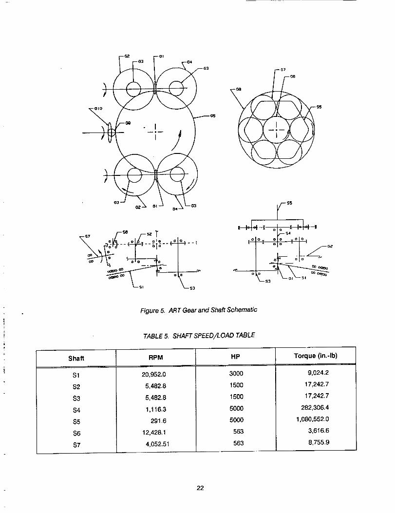
, I j
oo °l° -- -_'_--
--G7
G6
G8
S5
L I--|-I ,_ 0(0 -¢ I-|-I JS4
,.olo. ,. o o_ .,.olo ,
Figure 5. ART Gear and Shaft Schematic
TABLE 5. SHAFT SPEED/LOAD TABLE
Shaft
$1
$2
$3
$4
$5
$6
$7
RPM
20,952.0
5,482.8
5,482.8
1,116.3
291.6
12,428.1
4,052.51
HP
3000
1500
1500
5000
5000
563
563
Torque (in.-Ib)
9,024.2
17,242.7
17,242.7
282,306.4
1,080,552.0
3,616.6
8,755.9
22

TABLE 6. GEAR SPEED�LOAD TABLE
Gear
G1
G2
G3
G4
G5
G5
G6
G7
G8
G9
G10
No. of Teeth
28
107
34
107
167
167
58
51
164
15
46
RPM
20,952.0
5,482.8
5,482.8
5,482.8
1,116.3
1,116.3
1,116.3
937.8
0.0
12,428.1
4,052.51
HP
3000
1500
1500
1500
5000
563
5000
833.3
5000
563
563
Torque (in.-Ib)
9,024,2
17,242.7
17,242.7
17,242.7
282,306.4
31,787.7
282,306.4
0.0 (Idler)
798,246.3
0.0 (Idler)
8,755.9
A A
B B
D
Figure 6. ART Plan View
23

Find
No.
1
2
5
6
7
8
9
10
11
12
13
14
15
16
17
18
19
20
21
22
23
24
25
26
Dwg
Zone
5A
6A
7A
4B
4C
4D
5E
5E
6E
6C
6B
7D
8D
3D
1C
6D
6C
6B
4B
3A
4B
3C
3C
4C
TABLE 7. ART DESIGN PARTS LIST
Qty Description
1 Assembly, Transmission
1 Assembly, Lower Housing
2 Assembly, Input Quill
1 Assembly, NOTAR Drive
Components
(2-15,35,59,73,75)
(18,28,33,39,48,67,69,
79,85,86)
(80,81,82,83,84,87,88,8
9,92,93,94,98,99,100,
101,102,103,104,113,
114,119)
(19,20,21,22,24,25,27,
34,40,43,68)
(29,30,32,44)
(17,31,66)
(16,72,78,120,121,122)
(70,71,74,76,77)
(36,54,55)
Notes
1 Assembly, Spur Gear Shaft
1 Assembly, Middle Housing
1 Assembly, Upper Housing
1 Assembly, Carder
1 Assembly, Sleeve
1 Assembly, Sun/Combining Gear
1 Assembly, Clutch
Assembly, Face-Down Face Gear
Assembly, Face-Up Face Gear
Assembly, Main Oil Pump
Assembly, Secondary Oil Pump
(37,38,41)
(91,95,96,97,105,106,
107,108,109,110,111,
112,115,116,117,118)
(49,50,63,64)
(45,46,49,50)
(51,52,53,57)
(58,60,61,62)
Material
Housing, Upper
Housing, Middle
Housing, Lower
Shaft, NOTAR Drive
Housing Cover
Gear, Face - NOTAR
Bearing, Ball, NOTAR
Sleeve
Screw, Self-Lok
Aluminum Alloy
WE 43 Magnesium
WE 43 Magnesium
4340 Steel
WE 43 Magnesium
EX-53 Steel
M-50 Nil Steel
4140 Steel
4140 Steel
#210
Goes
Into
7
6
2
4
4
4
4
4
4
24

TABLE 7. ART DESIGN PARTS LIST (Continued)
FindNo.
27
28
29
3O
31
32
33
34
35
36
37
38
39
40
41
42
43
44
45
46
47
48
49
50
51
52
53
54
55
56
57
58
59
DwgZone
4B
5A
5C
5B
5C
4B
5C
3C
6E
6E
6A
5A
5A
3A
5A
3A
4C
8D
8B
3D
3D
8A
3C
2C
2C
4F
5E
2C
1C
7C
Qty Description Material
1 Nut, Self-Lok 4140 Steel
1 Bearlng, Roller, NOTAR M-50 Steel
1 Bearing, Ball, NOTAR Idler M-50 Steel
1 Nut, Self-Lock 4140 Steel
1 Bearing, Roller, NOTAR Idler M-50 Steel
1 Screw, Self-Lok 4140 Steel
1 Liner, Bearing M-50 Steel
1 NOTAR Drive Flange 4340 Steel
1 Retainer 4140 Steel
1 Bearing, Ball, Mast Support SAE 52000 Steel
1 Bearing, Roller Set, Combining Gear M-50 Steel
1 Gear, Combining/Sun M-50 Steel
1 Race, Inner M-50 Steel
1 Seal, Double Lip Speclal
1 Retaining Ring 301 Stainless
1 Cap Screw Retainer Steel
1 Gear, Spur- Idler EX-53 Steel
1 Gear, Face-Up Face EX-53 Steel
1 Plate 4340 Steel
2 Bearing, Ball, Face Gear M-50 Steel
1 Roll Pin Steel
1 Coupler, Splined 4340 Steel
1 Housing, Pump WE 43 Magnesium
1 Pump, Main Lube Gerotor 10 GPM
1 Shaft, Splined 4340 Steel
1 Sleeve 4340 Steel
1 O'Ring
1 O'Ring
1 O'Ring
4 Nut, Self-Lock 4140 Steel
Notes
#305
#308
#306
Special
Special
#217
GoesInto
4
2
5
5
6
5
2
4
I
I
10
10
2
4
10
4
5
13
13
2
12,13
12,13
14
14
14
9
9
14
15
1
25

TABLE 7. ART DESIGN PARTS LIST (Continued)
FindNo.
6O
61
62
63
64
65
66
67
68
69
70
71
72
73
74
75
76
77
78
79
80
81
82
83
84
85
86
87
88
89
90
91
DwgZone
1C
1C
1D
7C
7D
2F
7d
4A
3E
4G
4G
4F
4E
4E
4E
3D
3D
4F
7D
8A
8A
7A
7A
7A
7A
7A
7A
7D
7A
7H
Qty Description Material
1 Pump, Secondary Lube Gerotor 1.5 GPH
1 Housing, Pump WE 43 Magnesium
1 Shaft, SplJned 4340 Steel
1 Plate 4340 Steel
1 Gear, Face-Down Face EX-53 Steel
4 Bearing, Roller, Face Gear M-50 Steel
2 Bearing, Ball - Face Down Gear M-50 Steel
2 O'Ring
2 O'Ring
6 Gear, Planet Pinion EX-53 Steel
1 Planetary Carrier EX-53 Steel
1 Seal, Split Lip
1 Spring Steel
6 Bearing, Spherical, Planetary M-50 Steel
t Gear, Ring EX-53 Steel
6 Cover 2024-T4 Aluminum
6 Screw Cap 6061 -T6 Aluminum
1 Adapter/Seal Ring 6061-T6 Aluminum
2 Sleeve, Bearing M-50 Steel
2 Nut, Self-Lock 4140 Steel
2 Gear, Input - Spur EX-53 Steel
1 Bearing, Roller, Input Quill M-50 Steel
1 Resilient Mount 4340 Steel
1 Anti-Flail Ring 4140 Steel
2 Cover, Access 6061-T6 Aluminum
2 Retainer 4140 Steel
2 Tube, Spacer 4140 Steel
1 Screw, Set Steel
1 Shaft, Input 4340 Steel
Notes
#3O8 Sp
#118
Special
#108
1 Spacer Steel 11
GoesInto
15
15
15
12
12
6
2
4
2
8
8
7
1
8
1
8
8
7
2
3
3
3
3
3
2
2
3
3
3
26

TABLE 7. ART DESIGN PARTS LIST (Continued)
Find
No.
92
93
94
95
96
97
98
99
100
101
102
103
104
105
106
107
108
109
110
111
112
113
114
115
116
117
118
119
120
121
122
DwgZone
7F
7F
7F
7F
7F
7G
7F
6F
6G
6G
7H
6H
7H
7H
7H
7H
7G
7G
7G
7G
7F
7F
7F
7F
7F
7G
7G
7A
6D
6D
6C
Qty
6
6
6
1
1
1
1
1
1
1
1
1
1
2
1
1
1
2
1
2
1
2
2
1
1
2
A/R
1
2
8
2
Description
Bolt, Hex
Washer
Thread Insert
Ratchet
Nut, Lock
Spring
O'Ring
O'Ring
Drive Flange
Cover, Retainer
Seal, Magnetic
Housing, Retainer Cap
O'Ring
Bearing, Ball, Input
Coupler, Splined
Synchronizer
O'Ring
Pawl
Bolt, Hex
Washer
Nut, Hex
Nut, Lock
Bearing, Ball, Clutch
Spacer
Sleeve
Retaining Ring
Washer
Tube, Lube
Tube, Lube
O'Ring
Tube, Transfer
Material
Cres
Steel
Steel
M-50 Steel
Steel
Steel
4340 Steel
4340 Steel
6061-T6 Aluminum
M-50 Steel
4340 Steel
M-50 Steel
M-50 Steel
Steel
Steel
Steel
Steel
M-50 Steel
4140 Steel
4140 Steel
4140 Steel
4140 Steel
41 40 Steel
Notes
#013
#110
Goes
Into
3
6
6
11
11
11
3
3
3
3
3
3
3
11
11
11
11
11
11
11
11
3
3
11
11
11
11
3
7
7
7
27
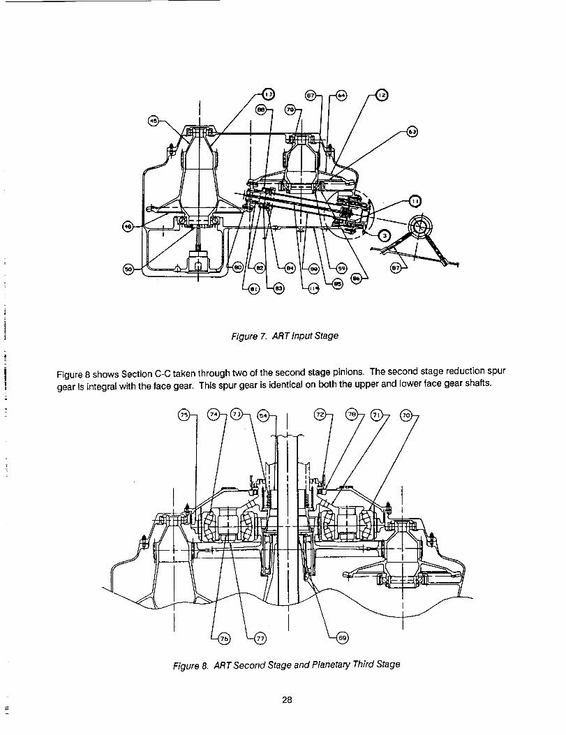
I @
Figure 7. ART Input Stage
Figure 8 shows Section C-C taken through two of the second stage pinions. The second stage reduction spur
gear is integral with the face gear. This spur gear is identical on both the upper and lower face gear shafts.
I I
II
II
II
!
I
Figure 8. ART Second Stage and Planetary Third Stage
28

Thus four pinions total, two on either side, combine to drive the collector gear which rotates at 1116 RPM. Thlsprovides a 4.912:1 reduction ratio at the second stage. The upper face gear shaft requires an E.B. weldbecause there is not enough clearance between the spur gear and the face gear web to grind the teeth. A
secondary web Is also welded on the upper and lower face gear shafts to provide a lightweight box structure forface gear stiffness.
The face gear webs and rims were designed to achieve neady equal radial, axial, and tangential stiffnessbetween the two. Matched web stiffnessresulted ina near equal torque split to the two face gears, as obtainedin a finite element static systems analysis. In addition, the magnitude of axial deflection, which occurs along theface gear tooth height, was limited inthe designs to approximately 0.005 inch. Thls represents less than 2percent of the tooth whole depth. Analysis showed the designs of both gear shafts effectively limit geardeflection while reducing weight and shaft length.
As shown in Figure 9, Section D-D, the transmlssion main lubrication pump is driven by the left hand lower facegear shaft and the emergency lubrication pump Is driven by the right hand lower face gear shaft.
Figure 9. ART Face-Up Face Gears/Lubrication Pump Drives
29

Thecollectorgearrecombinesthepowerfromtheupperandlowerfacegearsandalsocombinesthepowerfromtheleft-andright-handengines.Thecollector in turn drives the NOTAR/accessory output and the integralsun gear for the high contact ratio (HCR) planetary. Figure 10, Section A-A, shows this section of thetransmission. The collector gear Is supported by a dual roller bearing set which is designed to handle the smallthrust load produced by gear tooth errors, torsional windup, and the gear weight. The roller bearing set wassized for OEI power which produces the larger bearing loading. In the twin engine operation, much of thebearing load Is cancelled leaving only the NOTAR/accessory loads to be reacted by the roller bearing set.
The final transmission reduction is a simple HCR planetary design with the sun gear integral with the collectorgear. Shown in Figure 10, six equally spaced planet idler gears orbit around the sun and drive the planetarycarrier. The carrier in turn drives the main rotor drive shaft through a grease-packed crown tooth splinecoupling. The planet pinions contaln double row spherical bearlngs which run on common spherical racewaysintegral with the planet pinions. The bearings are self-aligning and thus Insensitive to misalignment of thecantilevered carrier posts. The flexured planetary ring gear provides controlled radial motion of the planets andis attached to the transmission housing at a bolted flange. The ring gear has no working spline to generate weardebris and isolates the meshing tooth noise from the housing at the bolt flange. The planetary is a high contactratio, dropped tooth design In which the sun, pinlon, and ring meshes have contact ratios of about 2.22, and thering gear action is almost fully recessed. The planetary is deslgned to employ the highest profile contact ratio
that can be gainfully used in a spur gear planetary drive. Table 8 compares a standard spur gear planetary witha high contact ratio planetary similar to the ART design described and notes a noise reduction of about 9.5 dB
[13]. Both planetaries given in Table 8 are sized to transmit the same torque with the same gear tooth bendingstresses. The dropped tooth gearing technique used permits the use of six planets at a ratio where normallyonly five could be used. The planet idler gears have two teeth less than what would normally be employed atthis ratio. This allows the ring gear to become smaller for the same reduction ratio, consequently reducingweight. The planet gears are equally spaced, but their tooth numbers provide a hunting ratio with respect to
their mesh with the sun and ring gears and allow the planetary system to be phased. Emphasis was placed onsystem-phasing the individual planet-gear mesh points and preventing all the pinions from meshing at the sametime. The system was phased so the sequences of engagement and sliding impulses between the six pinionscancelled. This eliminated external force or moment reactions. This method has demonstrated noise
reductions of up to 11 dB [14].
The final planetary design evolved from a trade-off study comparing two different planetary concepts primarily toconsider weight, noise and reliability. The baseline configuration, shown in Figure 11 centered around a rigidcantilevered planetary containing six planetary pinions with integral single row cylindrical roller bearings. Thebearings contained fourteen 30x42 mm rollers closely housed in a steel cage. The cantilevered carrier for thebaseline planetary was designed using finite element modeling with a goal limiting deflection of the cantileveredplanet pins to 0.001 inch per inch of length at maximum load. This value was chosen to maintain line contact onthe cylindrical rollers. A conical web directly connects the carrier plate to the hub. The cylindrical I-beam abovethe plate is required to resist planet pin deflection, The carrier material is carburized AMS 9310, chosen for theintegral splined crown tooth coupling required to drive the main rotor mast. Because the design criteria was
stiffness rather than strength, the stresses are extremely low and the weight is almost double that of thealternate carrier design. The baseline planetary gearing consists of a 58-tooth sun gear integral with the 167-tooth collector gear driving six 53-tooth planet idler pinions. The ring gear has 164 teeth which yields aplanetary reduction ratio of approximately 3.83:1 at a 7.500-inch center distance. The gearing has a 25-degreepressure angle and operates at 7.400 diametral pitch. The gears have standard tooth proportions with the face
widths sized for infinite tooth bending strength at 100 percent power. This yielded L10 pitting lives which greatly
exceeded the 15,000 hour component life requirement for life equivalent power.
3O

Figure 10. ART Combining Gear,/NOTAR Drive and Planetary Stage
Standard (XV-15 Final Stage)Spur Gear Planetary Design
High Contact Ratio (Model 222)Spur Gear Planetary Design
TABLE 8. PLANETARY COMPARISON TABLE
II Weight (Ib)
4O
38
FEfficiency (%) Noise (dB)
r
99.7 X
99.4 X -9.5
Life
X
2X
The alternate planetary design analyzed in the trade-off study is described at the beginning of this section. Thisconfiguration was selected as the final design because of the weight savings advantage and the potential toreduce the noise level with no decrease In gear or bearing life. The alternate planetary gearing consists of a 58-tooth sun gear integral with the 167-tooth collector gear driving six 51-tooth planet idler pinions. The ring gearhas 164 teeth which yields a planetary reduction ratio of about 3,83:1 at a 7,500-inch center distance, The sun-pinion mesh has a 16.01-degree pressure angle and operates at 7.533 diametral pitch. The gear toothproportions are 37,8 percent greater than standard tooth proportions with the face widths sized for infinite tooth
bending strength at 100 percent power and well over 15.000 hours L10 pitting life at the life equivalent power.
Table 9 gives a comparison between the baseline planetary design and the high contact ratio planetary design
selected. A detail weight analysis indicated a difference of 68.5 Ib between the two planetary stage designs withboth falling under the parametric ART weight allocation.
31

w

SHAFT
SUN
_LANET PLANET PIN
PLANET CLAMPING BOLT
(LEFT HAND THREAD)
Figure 11. ART Baseline Planetary Design
Standard
Planetary
High Contact
Ratio Planetary
TABLE 9. BASELINE PLANETARY VERSUS HIGH CONTACT RATIO PLANETARY DESIGN
Contact Fitting Face Contact
Ratio L1 Life Width Efficiency Temperature
1.59
2.22
> 10,000 hrs
> 10,000 hrs
3.93 in.
3.25 in.
99.93%
99.85%
267.1 °F
337.5 °F
The NOTAR spur gear idler is driven from the collector gear at a speed of 12,428 RPM and provides the speed
up ratio required for the NOTAR face gear. The NOTAR face gear drives the NOTAR and the accessory gearbox
and is attached to the bolted flange output shaft with a double piloted splined connection. The face gear has a
speed reduction ratio of 3.067:1 which is about the smallest reduction ratio possible to retain an adequate tooth
profile on the face gear. The face gear angles the output shaft along the 0.00 aircraft waterline and provides a
N©TAR shaft speed of 4,052 RPM. The NOTAR shaft is on the centerline of the transmission.
32


The transmission attachment and main rotor drive configuration is identical to the AH-64 Apache helicopterdesign, whereby the transmission housings are designed to handle drive loads only and the rotor loads aretaken out through the mast support structure. This feature not only minimizes weight and increases reliability,but allows the transmission to be removed from the aircraft in a simple manner without disturbing the rotor orthe controls. The transmission is simply supported from the top by tension bolts with the torque being reacted
by a curvic type coupling. The drive shaft from the main transmission to the rotor Is a full-floating-type unithaving grease lubricated spherical gear couplings at each end. It Is supported from the top and provides torquetransmission only and accommodates the small angular mlsalignment of the transmission to static support andthe static support to rotor.
The transmission housing is a three-piece housing bolted together as an assembly. Figures 12, 13, 14, 15, and16 show outside views of the ART housing. The housings are proposed to be manufactured from ElektronWE43 high-strength, corrosion-resistant sand castings. The housings contain internal cored passages forlubricant transfer. The choice of housing material was made after a preliminary trade-off was conducted lookingat weight, corrosion resistance, strength, method of fabrication, and fatigue characteristics.
The lubrication system for the ART is schematically shown on Lucas Western Drawing 42499-1037, shown hereas Figure 17. The system is self contained, except the external heat exchanger. The lubrication system is anextension of current practice. The extension is directed toward taking advantage of advanced technologymaterials and components. These materials and components allow an oil-out temperature from the gearbox of400°F and an oil-in temperature from the oil cooler of 230°F. This allows a 10 gallon per minute (GPM) pump
where conventional practice for a 5000 HP transmission would require 27 GPM. Conventional practice uses a16 second cycle time, which would require 7.2 gallons of oil for the 27 GPM case versus 2.2 gallons for our 10GPM case which uses a 13 second cycle time. At 7.6 pounds per gallon, a direct savings of 38 pounds resultsplus added savings from a smaller system. Cycle times as short as 8 seconds are being used successfully sothe 13 second cycle time is somewhat conservative.
Figure 12. ART Aft View of Housing
33

\
Figure 13. ART Plan View of Housing
Figure 14. ART Profile View of Housing
34

Figure 15. ART Transmission Case, Tri-Metric View Looking Down
Figure 16. ART Transmission Case, Tri-Metric View Looking Up
35

i
J
o
m!.,.i
--z 1
I
1
= I _" l _ T = ]" _ ]" © T
+
4
36

The benefits of using high oil temperature carry over into the oil cooling system. The greater the difference in oiland air temperatures, the more heat is rejected directly by the gearbox. The higher the allowable oiltemperature out of the cooler, the smaller the alr/oil heat exchanger. Taking both these factors into accountresults in an oil cooler having a core weight of 17 pounds when optimized with respect to pressure drop through
the cooler, air flow, air pressure, blower power, and blower weight.
A conventional design using 27 GPM, 275°F oil out of the gearbox, 205°F oil out of the cooler and the same airtemperature of 125°F results in a core weight of 61 pounds. Oil weight savings and core weight savings is 82pounds directly. The total weight savings from secondary effects would be considerably higher.
A third approach of interest is the provision of emergency lubrication after oil is lost from the gearbox. It isplanned to provide a constantly filled separate oil tank within the gearbox which feeds a 1.5 gallon per hourpump. The oil is delivered under pressure to three mist jets, one on each input plnlon, and one directed into thezone between the comblning gear and the output planetary. The system Is designed for over one hourendurance and is entirely Independent of the primary oiling system. It operates all the time, and provides a
signal if it becomes inoperative. The basic concept is that either oil system will function independent of loss ofoil in the other.
The lower part of the transmission acts as the lubricant sump and has an approximate capacity of 500 cubicinches. The oil circuit is described later In this section.
Starting at the sump, oil passes through a 400 micron screen into a 4065 gerotor lube pump which has acapacity of 10.0 GPM. At thls point, the system contains a high pressure relief valve set at 200+10 PSID. Thehigh pressure relief valve protects the system by limiting excessive pressure due to very cold oil or otherreasons. The oil then enters a Tedeco Lubriclone Deaerator with a quantitative debris monitor (QDM), Part No.1P 1284. Entrained air is removed by the lubriclone which delivers solid oil to the QDM
QDM is a technology for determining the operating condition of oil-wetted mechanical parts such as bearingsand gears. Abnormal wear and mechanical damage can be detected well in advance of complete mechanicalfailure. Measurement of debris particle generation rate within certain particle size categories provides the
information necessary to detect the onset of failure in time to take corrective safety action and trend informationrequired to implement a cost-effective maintenance and repair program.
The QDM sensor is located in the lubrication system where it is exposed to the entire lubricant flow to assuremost effective capture of damage debris and early notification of impending failure. The QDM sensorincorporates a magnet to attract and capture ferrous debris and a coil which generates a voltage pulseproportional to the magnetic flux disturbance caused by the capture of the debris. This design approach hasthe advantage of not only signaling the existence of debris, but also retaining the debris for subsequent analysis.Since the magnetic flux disturbance is a function 0fthe mass of the debris particle, the resultant signal
amplitude indicates the size of debris captured by the sensor. The signal conditioner contains built-in testcircuitry. The circuit is activated by a pushbutton on the unit and generates a pulse simulating a large chip.
Oil exits the QDM through a 250 micron barrier screen. The barrler screen prevents foreign objects fromentering the QDM when the external line is not present. "Fhe barrier screen also prevents non-ferrous debris,
which can escape the QDM, from entering the oH cooler. The screen is removable to allow inspection foraccumulation of non-ferrous debris. The pressure drOp through the Lubriclone/QDM is 15 psi.
37

Theoil cooling system has been optimized by the Janitrol Aero Division of FL Aerospace, Part No. POS 39101,INP. The design features a 17.25 pound core measuring 12-1/8 x 3 x 20 inches. The heat load is 6600Btu/minute, 400°F oil in, 230°F oil out. The cooler passes 10 gallons of oil/minute with an 11 PSI drop.Cooling requlres 165 pound/minute of 125°F ambient air furnished by a 7 HP 8 pound fan. The cooler has a
low temperature by-pass and a high pressure by-pass which induces a 40+_5psi drop.
After the oil exits the cooler it passes the high temperature warning switch, set at 250°F minimum, which willindicate an oil over-temperature condition.
The oil then enters the filtration system, Aircraft Porous Media Part No. AEB 667-10Y3. Three micron filtration,which has demonstrated significant advantages and has been widely adopted in helicopter engines and
transmissions, is provided. The basic concept is that particles smaller than 3 microns are smaller than thethickness of the oil film which separates'gear teeth and rolling elements in bearings from the bearing races. Toover simplify, since wear is generated by debris, if the debris is removed, there will be no wear. This has provento be generally true. By actual test, oil service life increased from 100 to 1000 hours, filter llfe after Initial clean-up Increased from 400 hours to 1000 hours, bearing life increased 100% with a potential for no fatigue limit.Three micron filtration also eliminates SOAP analysis. The filter includes an impending bypass indicator withswitch, bypass with switch and a low temperature lockout. The filter has a 15 PSI drop while the bypass has a30+5 psi drop. Oil then passes to multiple jets which direct and meter oil flow, as needed, to lubricate and cool
the transmission gears, bearings and splines. Jets orifice size will be 0.030-0.034 inches. It is estimated that 30to 40 iets w#_be used for a totaJ fJow of 5.4 to 9.3 GPM. Each jet Jsprotected by a 250 micron contaminantbarrier screen. A low pressure relief valve, set at 80+5 PSID, is included in this part of the oil circuit andestablishes pressure at the lube Jets and bypasses excess oil to the sump. The last monitor before the return tothe sump is the low pressure warning switch, set at 40+5 psi.
The sump return line terminates in a nozzle directed into an eductor, or jet pump, inlet. The eductor inlet is infact the oil pump inlet. This technique accelerates sump oil into the pump inlet, reduces entrained air into thepump and will compensate for a low oil condition by reducing sump dwell time. In fact, this technique Is used inone application with a dwell time of 8 seconds.
The oil is added to the transmission via a filter cap with breather. The breather has a flapper valve to let air in
through a desiccant filter or air out as required by pressure changes. The desiccant filter is intended to reducewater entering the gearbox through the air inlet. Even minute amounts of water can cause damaging rust andaccelerate crack growth.
The filter cap leads to the eme(gency !ube tank which overflows Into the main sump. The sight gage monitorsthe oil level in the main sump. Thus both tanks are full when the sight gage indicates full. The main sumpcontains a low oil level switch in addition to the sight glass. The main sump is drained by a non-magnetic drain
plug because all ferrous debris must be routed to the QDM.
The emergency lube system is a separate entity. The gearbox contains a closed internal tank fed by one of thestandard oil jets at 10.8 gallons per_hour. The internaltank contains 400 cubic inches. Overflow oil is returnedto the main sump. From the emergency tank, the oil goes throughal00 micron screen into a 10010 gerotor
pump delivering 1.5 gallons per hour to three mist ietms, LEE Part No. NZA 180118H. Each jet uses 0.5 gallon perhour. One jet is directed at each input pinion and one jet is directed into the zone between the combining gear
and the planetary. Theemergency lube system operates continuously and has over one hour endurance. Theemergency lube circuit contains a low pressure switch set at 40 psi which operates a shut-off valve controlling
the jet feeding the emergency Jube tank. This switch aJso sends a signal that the emergency lube system Js
38

inoperative.Ferrousparticlesentering the emergency lube tank cannot be allowed to escape. Therefore this
tank has a magnetic drain plug to capture debris that might damage the pump.
Both the primary and emergency pumps are driven by shafts connected to first stage gears. Therefore no gearsor bearings are added to the transmission to drive the oil pumps.
In summary, there are seven lubrication system sensor components that provide transmission conditionmonitoring signals. These are:
Sense
Quantitative Debris Monitor
High Temperature Switch
Filter Element Switch
Impending Bypass Switch
Bypass Switch
Low Pressure Switch
Emergency Lube Low Pressure Switch
Indication
Abnormal wear
Oil cooler malfunction, low oil supply, oil leak
No filter element present
Filter collecting debris
Filter plugged, oil contamlnated
Low oil, oil leak
Emergency oil low or leaking
The seven switch signals can be provided as cockpit warnings of each condition sensed; or, ganged to provideone transmission problem signal. The concept behind one transmission problem signal is that a combat aircraftshould be designed to refuel and rearm with as little maintenance as possible. Either all systems are ready ornot ready with no panel openings and ground inspection required. Certain signals may also be used for
maintenance status panels, if provided on the aircraft. It is the responsibility of the aircraft systems integratorsto decide what, and how, to display transmission condition monitoring signals for the cockpit crew andmaintenance personnel.
IV.B GEAR ANALYSIS
Structural analyses for the gear components were performed in support of the Advanced RotorcraftTransmission (ART) Design. Analyses of the gear tooth bending stresses, the compressive (Hertzian) stressesand the scoring risk evaluations were conducted. All the gear components in the main transmlsslon as well asthe NOTAR and accessory power drive were analyzed.
The gear tooth stress analyses for the spur gear components were carried out per AGMA standards. Due to the
unusual geometry of the face gear [15], the formulas are not available in any of the standards for stress analysis.An approximate method for analyzing the face gears is used In the first stage and the NOTAR/accessory powerdrive gear analyses. This method tends to give conservative values of both tooth bending and compressivestresses. The results of the gear tooth stress analyses are tabulated in Tables 10 and 11.
39

TABLE 10. SUMMARY OF GEAR STRESS ANALYSIS
Stage Part
1 Pinion
1 Face Gear
2 Pinion
2 Gear
3 Sun
3
3
3
NOTAR
NO. of
Teeth
NOT/_R
28
107
34
167
58
Bending
St (psi)
36,112
< 36,112
Compressive
S¢ (psi)
143,590 (@)
52,142
143,590(@,!15&531
Load (HP)
150o (OE01500 (OEI)
43,292 1500 _OE_
40,787 158,531 1500 (OEI)158,9OO
Planet(#}. 51 41,760 158,90051 45,941 122,603Planet(#)
Rin9Gear
NOTAR Idler
Idler
NOTAR Face Gear
48,307
12,637
164
167
122,603
152,512
152,51215
15
19,017
5000/6, MCP
5000/6, MCP
5000/6, MCP
50OOl6,MCP563* (71%)563 * (71%)
23,317 177,857 (@) 563 * (71%), .=
46 < 50,896 177,857 (@) 563 * (71%)# Bending stress should be divided by a factor of 0.7 to account for the effect of reverse bending on the
planet.@ The compressive stress for the face gear drive is the value calculated at the pitch point,
which is closer to the test results.
TABLE 11. SUMMARY OF ART GEAR DESIGN LIFE VALUES
GearsItem No.
-081
-012
-012
-013
-013
-010
-010
-010
-070
-070
-075
-005-005
-021
Description
In.put Spur Pinion
Upper Face Gear
Collector Pinion (2)Lower Face Gear
Collector Pinion (2)Collector Gear
Collector Gear - NOTAR Mesh
Planetary - Sun GearPlanet Gear- Sun Gear Mesh
Planet Gear - Rin_] Gear Mesh
Rin_ GearNOTAR idler Gear - Collector Mesh
NOTAR Idler Gear - Face Gear Mesh
NOTAR Face Gear
NOTES:
Oty2
2
2
2
2
1
1
1
6
6
1
1
1
1
RPM
20,952.0
N0. of
Meshes I HertzStress
99,478
Load
(HP/mesh)
1,000
L10 Life
(hrs)
1.5E+08
5,482.8 1 99,478 1,000 1.2E+09
5,482.8 1 131,002 1,000 8666102
5,482.8 1 99,478 1,000 1.2E +09
5,482.8 1 131,002 1,000 8666102
I, 116.3 4 131,002 1,000 10641070
1,116.3 1 152,512 .71"563 2818434
1,116.3 4.432 142,124 666.7 2241069
902.41 1 142,124 666.7 12287599
902.41 1 101,854 666.7 4.7E+09
291.63 6 101,854 666.7 2.4E+09
12,428.14 1 152,512 .71"563 253152.8
12,428.14 1 150,909 .71"563 305722.1
4,052.65 .71"563150,909 937549.0
(1) A factor of 1.389 is used to account for the high contact ratio of the face gear drive.
(2) Calculated gear L10(L1) life and cycles are based on AGMA compressive stress.
(3) Life equivalent power per engine = 80%* (single engine MCP) = 0.8 * 2500 HP = 2000 HP
Life equivalent power for NOTAR and accessory drive = 0.71 * 563 = 400 HP
(4) AGMA compressive stress allowable of 225,000 psi for 107 cycles and .99 reliability is used in lifecalculation.
40

IV.C BEARING ANALYSIS
This section summarizes the bearing life analyses for the bearing components in ART design. The design lives
(B10) for the bearing components are aimed at 15,000 hours. A Life Equivalent Power (LEP), which is equal to
67 percent of the Maximum Continuous Power (MCP), is used for the bearing life analyses.
The ball and cylindrical roller bearing lives are calculated using the "Rolling-Element Bearing Analysis Program"
developed by A.B. Jones, Newington, Connecticut. Table 12 gives the bearing lives calculated. The lives
reported are the adjusted lives using the EHD film thickness life adjustment factor. The total life adjustment
factor for the bearings associated with main transmission gear shafts ($1 through $4) is 12.0. The factor Is a
combination of a material factor of 2.0, a process factor of 3.0, and a life improvement factor of 2.0 for the use of
the three micro filter. All other factors are considered to be 1.0. In analyzing the collector-to-sun-gear shaft
($4), the Ioadings are balanced under an even twin engine input condition. Therefore, the size of the bearings
are designed for a more critical OEI condition.
TABLE 12. ART BEARING DESlGN AND CALCULATED LIFE VALUES
Find
No.
114
105
82
B10
Qty Descriptions RPM Hours
4 Input Shaft Bearing: Duplex Ball, Clutch 20952 >50000
4 Input Shaft Bearing: Duplex Ball, Adapter 20952 >50000
2 input Shaft Bearing: Roller, Input Quill 20952 >50000
48
66
2 Face-Up Gear Shaft Bearing: Ball, 217B 5483 28315
2 Face-Up Gear Shaft Bearing: Roller, 308R 5483 22484
67
66
36
37
37A
74
2 Face-Down Gear Shaft Bearing: Ball, 118B 5483 44256
2 Face-Down Gear Shaft Bearing: Roller, 308R 5483 21926
1 Collector Gear $4 Bearing: Ball 1116 >50000
1 Collector Gear $4 Bearing: Roller, 121R 1116 >50000
1 Collector Gear $4 Bearing: Roller, 021R 1116 >50000
6 Planet Spherical Roller Bearing 902 16629
31
29
1 NOTAR Idler $6 Bearing: Roller, 306R 12428 20014
1 NOTAR Idler $6 Bearing: Ball, 308B 12428 14735
28
22
1 NOTAR Output $7 Bearing: Roller, 305R 4053 31379
1 NOTAR Output $7 Bearing: Duplex Ball, 210B 4053 39409
41

The supporting bearing for the idler and output shafts (S6 and $7) Is also analyzed using A.B. Jones' Computer
program. A combined material, process and life Improvement factor of 22.0 [16] is used for VlM-VAR M-50bearing material in the bearing life analyses of NOTAR and accessory power drive.
The bearings of the engine Input shaft ($1) theoretically are not loaded by any bending moment or radial forcedue to the split torque configuration of the ART design. This assumption is based on the ideal condition that the
torque is evenly divided into the two output shafts. The flexural mounting design for the engine input shaftsupport at the front end allows for nearly even torque splitting. Another ART design advantage results from theapplication of face gear drives using a spur pinion to drive the generated face gears. No thrust load isgenerated in this type of gear meshing. Therefore, the bearing lives (B10) of bearlng components associatedwith the engine Input shaft are conceptually determined to be higher than 50,000 hours.
The planet spherical roller bearing lives are calculated using the PLANETSYS computer program and the NASAmodel. The lives reported are the adjusted lives. The computer program's film thickness lubrication lifeadjustment factor was modified from 0.21 to 3.0. This is based on the paper "Life Adjustment Factors for Balland Roller Bearings," sponsored by the Rolling-Elements Committee and verified by helicopter transmissionexperience. The total life adjustment for the spherical roller bearing is 3.6. The factor of 3.6 is set using amaterial factor of 2.0, a process factor of 3.0, a lubrication factor of 0.3, and a life improvement factor of 2.0. Allother factors are considered to be 1.0.
IV.D GEAR SHAFT STRUCTURAL ANALYSIS
Structural analyses of the gear shafts were conducted in support of the ART design. Static analyses were
performed at critical cross-sections of all gearshafts, shear force and bending moment diagrams wereconstructed using the gear meshing loads and the reactions at the bearings as input. The reactions at the
bearings were derived from high speed roller bearing analyses using the A. B. Jones program. The analyses, ingeneral, showed high margins of safety for each gear shaft in the current design.
Because of the complexity of the conical-box shaped gear blank design and the concentrated applied loads atthe edge, the deflections and the maximum stresses for the face-down gear shaft and the face-up gear shaft cannot be easily solved by equations. Analytical methods for evaluating the strength and the stiffness of the conicalplate or the conical box configurations are commonly required in bevel type gear design, face gear drive(loaded by the separating force), and the helical gear design (loaded by the thrust force). Therefore, a
parametric study of the gear blank structures using the finite element method was conducted. Fatigue analyseswere carried out for the ring gear structure, which is subjected to cyclic load In normal operation. The analyseswere conducted at the planet spindle and at the critical section near the lubrication holes of the carrier plate.
Design criteria used In performlng all analyses are listed below.
IV.D.1 Design Criterlaand Loads for Gear Shaft Analysis
Ultimate HorsePower:
a. Ultimate HP for the first stage is based on (OEI Power) * 1.5
OEI Power: One Engine Inoperative HorsepowerMCP: Maximum Continuous HorsepowerOEIPower = 1.2*MCP = 1.2*2500HP=3000HPUltimate Power = 3000 HP * 1.5 = 4500 HP
42

b. UltimateHPforthe combining stage and the planetary stage Is (twin engine MCP) * 1.5
5,000 HP * 1.5 = 7,500 HP
c. _Ultimate HP for the NOTAR and accessory drive
563 HP * 1.5 = 844.5 HP
Fatlque Analysis:
For adequate fatigue strength, gearshafts are to be designed for infinite life at the following loads:
a. For Gear Shafts $1, S2, and $3
(50% + 50%) * (OEI Power)(50% + 50%) * 3000 HP = 1500 HP + 1500 HP
b. For Gear Shafts $4, $5 and Other Planetary Stage Components
(50% + 50%) * (twin engine MCP)(50% + 50%) * 5000 HP = 2500 HP + 2500 HP
c. NOTAR and Accessory Power Drive (Shafts $6 and $7):
(50% + 50%) * (NOTAR/Accessory Drive MCP)(50% + 50%) * 563 HP = 281.5 HP + 281.5 HP
Such a loading also represents the GAG (ground-air-ground) condition as the spectrum for fatigue lifecalculation.
Material Properties:
The material properties for 9310 Steel, CEVM per AMS 6265, Rc 33-41 Core used in AH-64 Drive System FatigueAnalysis are
Ftu = 150 ksi
F = 90 kstsu
F = 30 ksi (design endurance limit)e
A summary of gear shaft stress analysis is shown in Table 13.
43

Table 13. SUMMARY OF GEAR SHAFT STRESS ANALYSIS
Components
Input Pinion ShaftMost critical shaft section
Spline section
Face-down Gear Shaft (FEA)
Web
Most critical shaft section
Face-up Gear Shaft (FEA)
Web
Most critical shaft section
Collector
Most
Most
Gear to Sun Gear Shaft
critical web section
critical shaft section
Planetary Stage, Ring Gear
Planet Carrier
Most critical shaft section
Most critical web section
Weight-reduction hole
Planet spindle
For all of the above
NOTAR/Accessory Power Drive, Idle Shaft
Most critical shaft section
NOTAR/Accessory Power Drive, Output Shaft
Most critical shaft section
Spline section
Type of Stress
Torsion
Torsion
Combined stress
Combined stress
Combined stress
Combined stress
Torsion
Torsion
Hoop stress
(fatigue)
Torsion
Torsion
Stress concentration
Bending
Fatigue
Combined stress
Combined stress
Torsion
Margin of Safety
+2.75
+2.35
+ 7.24
+11.5
+ 16.22
+11.5
+ 4.65
+ 2.45
Sal t < Fe(* )
+1.186
+ 1.62
+ 1.06
+4.47
Sal t < Fe
+6.747
+ 1.07
+ 0.783
Note: (*) Sal t
Fe
Calculated alternate stress
Adjusted endurance limit (considering the effect of mean stress)
44

IV.E MASS PROPERTIES ANALYSIS
IV.E.1 Introduction
This report details the history and results of generating the weight estimates for the Advanced RotorcraftTransmission (ART) design concept formulation. Parametric weight estimation methodology was used to size
the design concept followed by a UGII volumetric mass properties analysis using the R800-0001 drawing file.This then was added to the main rotor driveshaft, static mast, lube system, and miscellaneous componentweights resulting in a total installation weight. The total installation weight for ART can then be assessed againstthe current status of the design. The latest weight status shows that there is still enough buffer to meet theweight goals.
IV.E.2 Summary Profile and Outline Qf ART Weight Goal_
The following summary table profiles the orlglnal drive system weight estimate prior to incorporating advancedtechnology, the ART weight goal incorporating the 25 percent weight reduction, and the current volumetricweight estimate.
The baseline helicopter is the Army AH-64 Apache upgraded to FAR requirements as described in the Baselinesand Allowables section. The industry weight trend for a 5000 HP helicopter main transmission with an Apachemain rotor speed of 289 rpm Is 1792 lb. This in turn results in a weight goal for the Advanced RotorcraftTransmission, with a 25 percent weight reduction, of 1344 lb. Additional component breakout as shown In Table14 is the result of approximating to the AH-64A Drive System component relative weights.
TABLE 14. ART WEIGHT PROFILE
Component
ART Transmission Assembly
Main Rotor Driveshaft
Static Mast
Lube System (not including oil)
Miscellaneous Components
OriginalParametric Weight
(Ib)
1347
143
112
120
7O
ART
Goal Weight(Ib)
1010
105
95
80
54
Current
Volumetric Weight(Ib)
815
115
102
83
55
Total Install Weight 1792 1344 1170
The parametric weight estimation methodology which was used to estimate the weight of the drive system
major components was derived and documented in Reference [7]. This methodology is based on a stage-by-stage dimensional analysis. The methodology used 39 gearboxes in the derivation process resulting in astandard deviation of 9.3 percent. The method estimates the weight of the gears, pinions, bearings, supports,and case (in effect, a 'dry gearbox'). The weight estimation methodology was correlated to the AH-64A maintransmission. The uncorrected weight estimate was 6 percent greater than actual.
45

A parametricweight check was performed using the Advanced Rotorcraft Transmission design and dimensionalinputs to generate a weight profile of the gearbox arrangement. A total composite of this analysis is shown onTable 15. This total weight (1036 Ib) Is equivalent to the ART transmission assembly weight goal of 1010 Ib (referto Table 14). The purpose of this exercise Is to show parametrically that with the dimensional inputs of the ARTtransmission assembly, the weight goal is achievable.
TABLE 15. ART TRANSMISSION ASSEMBLY PARAMETRIC WEIGHT CHECK
PARAMETRIC WEIGHT CHECK SUMMARY SHEET
Component
Input Stages (2)Input Gears** (2)Comblnlng Gear (1)Combining Gear Pinions (3)Planetary (1)
Weight (lb)
147.0111.4243.5117.8416.7
Total Parametric Weight 1036.4
**Input Gears weight determined by the following operation:
Input Stages (2)Remove Input Pinions (2)
Input Gears (2) 111.4
IV.E.3 Volumetric WejQht Analysis
A volumetric weight analysis was completed using the existing ART Unigraphics model (R800-0001). Theapproach taken was to analyze only those components which were comparable to the parametric equation.Components calculated include all main transmission gears, pinions, associated bearing assemblies withsupports, and the Case surrounding these components. The components calculated (ART transmissionassembly) represents approximately 70 percent of the total installation weight.
The general procedure followed to obtain the component volume for weight calculations Is as follows. Amajority of the transmission components are currently modelled in 2D only. To obtain volumes, those partswhich were symmetric were revolved about their axis. These parts Included all gears, pinions, shafts, bearings,bearing races, etc. For those parts which were not symmetric, in particular the housing, a cross-sectional areawas obtained and then extended the appropriate length to obtain the volume.
To save time, some compromises were made in the volumetric analysis. For example, those component areas
which contained numerous fillets and bends were simplified with straight line segments. For those components
which were non-symmetrical, average cross-sectional areas were sometimes taken. An attempt was made tonever remove material with these approximations. Depending on the complexity of the component and number
of approximations used, a percentage of the calculated volume was added to account for undefined areasbefore the weight calculation was performed.
46

IV.E.4 (_on_tlt_sions
The current status of the ART mass properties is shown inTable 16.
TABLE 16. ART VOLUMETRIC WEIGHT SUMMARY
Component
ART Transmission AssemblyMain Rotor DriveshaftStatic Mast
Lube System (not Including o11)Miscellaneous Components
Total Installation Weight
Installation Goal Weight
Weight buffer to Date = 15%
Current Weig ht(Ib)
815115102
8355
1170
1344
Table 17 provides a detailed weight breakout for the transmission assembly weight shown In Table 16.weights shown were generated through calculations on the UGII from drawing R800-O001. Additionalinstallationweight increases of 10 percent were Included and noted on Table 17 as appropriate.
All the
47

t- C C i- e-" C=
4. + ÷ Jr + ÷
1-.. _P
LLI
C_ ]
48

49

ILl
- _ • • _ o o 2 _ _ _ o o d
....... d d d d o d d d d
,.,.J
50

j ,,¢=
• mE
U.I
:Z:
I,-..
I<
LLI-4
c_
_J o b b z ,, ",- _ ,_ o b ,',
51

J0
n
0
c_
_L
ILl..,.Ic_
52

_ o o d c_ d ,-: d d d o d _ c_ o c_
{_ 8 _ s 8 8 _ _ _ 8 s _ _ 8 8 8o o .o o o _ o o o o o _ d o
_ _ o o o d o d d d d d d d o d o
LU121
...4
58
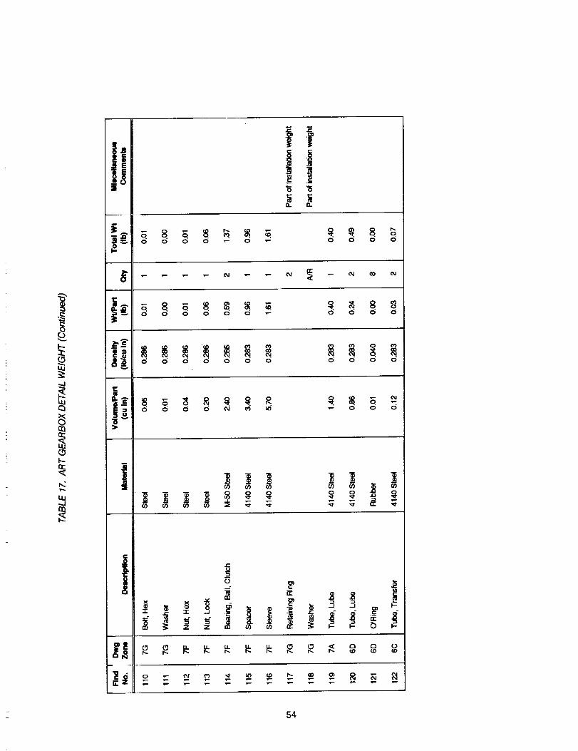
"6 "6
a. o,.
o o o o
o o o o
. 04,0 0 0 0
Q
b..
laa
i
3
o _
z z _ -" _ _ _- b _-
54

IV.FSUPPORTABILITY
IV.F.1 Abstract
This section presents the supportability analysis of the Advanced Rotorcraft Transmission (ART) design.Supportability includes Reliability, Maintainability, Survivability/Vulnerability (S/V), and Integrated Diagnostics.The ART program has a reliability goal of 5000 hours Mean Time Between Removal (MTBR). The plan to attain.that reliability is outlined as well as an assessment of the ART MTBR. Strategles for Increasing reliability duringproduction design are presented. Maintainability, Integrated Diagnostics and Survivability/Vulnerabilityassessments were completed.
IV.F.2 Introduction
There is a high degree of interrelationship between all design criteria, so a formalized systems approach istaken. This approach is based on the evaluator function, a mathematical model for doing trade studies [17].The evaluator function provides perspective for choosing design trades. An example of this Is the relative meritof a high maintainability/low reliability vs. high reliability low maintainability applied to seal selection.
Supportability Includes features of the design that have the highest effect on the operational phase. This phasecontains the bulk of the life cycle costs of the unit as shown in Figure 18. To reduce costs, military andcommercial customers are paying increasing attention to the supportability features of the design.
Supportability
--- Ufe CycleCost .:
: -_ Operation and Support -:
-. System Acquisition -.." r-'-"/ :
: : • _v _ :
: , Production _, :
•:._System Resea " :
: and Development : _V _
,
: •
i so'/. .:
: 30% :
10%
A A A A
0 I II III YearsMilestones
Figure 18. Nominal Cost Distribution of a Typical DoD Program
55

The following sections focus on the individual disciplines within supportability. They are followed with adiscussion of how the individual conclusions relate to one another. The eady analysis has been preserved to
document the basis of the design decisions. This will be useful during the pre-production design andmanufacturing stages In that changes will be made with awareness of the design intent. Loss of deslgn Intent isa major Issue in concurrent engineering [17].
IV.F.3 Reliability
In the effort to meet weight and performance goals with any given technology, there Is a trade-off with reliability.Every excess pound of unnecessary material reduces available payload. Where can design reduce weight andnot affect reliability?. Which configuration has the best prospects from a reliability standpoint? Transmission
design Is such that any degree of reliability can be achieved by sacrificing weight, performance and cost.MDHC's method for achieving the reliability goals for the ART was to engineer them in through:
, Using the established Failure Modes, Effects, and Criticality Analysis (FMECA) procedures (seeAppendix B2). Although this is not a production effort, the groundwork Is laid for detail reliability
evaluation. By staying consistent with the FMECA process, we are ensuring continuity in reliabilitysupport should the design go into production.
. Ustng concurrent engineering [feed-forward (reliability apportionment) and feed-back (reliabilityevaJuation)cycJes|.
, A high degree of communication between designer and engineer during the conceptual deslgn.This is facilitated electronically where efficient, i.e., E-mail.
4. Use of Computer-Aided Engineering codes to automate analysis as much as possible.
The strategy is to base ART reliability on AH-64A reliability. AH-64A reliability is analyzed by failure mode.Prospective Improvements designed to reduce selected failure modes are sought and analyzed for their overallimpact on the design.
IV.F.3.i Measures of Reliability
Reliability Is a critical attribute of helicopter transmissions. There are many measures and criteria of reliabilitythat a transmlsslon must meet. The main criteria used by the military are misslon reliability and systemreliability. These two criteria are very useful in understanding how an aircraft is performing.
1. Mission reliability is the measure of mission time units (typically hours) divided by the number ofcritical failures during a stated series of missions. This would include chip lights, high-temperaturelights, and failure of basic drive components.
. System reliability is a basic measure of reliability for repairable items: the mean number of life unitsduring which all parts of the item perform within their specified limits, during a particularmeasurement interval under stated conditions. Note that this includes all mission-critical failuresand non-critical failures such as loss of redundant units and non-critical Indications.
56

ARTTASKI11,missionanalysisreportssignificantimpactoftheARTtransmissionto thehelicopter'sreliability.Atthisdesignstageweareinterestedprimarilyintransmissionmissionreliability,usingsystemreliabilityandMaintenance-Man-Hours-per-Flight-Hourasatrade-offmeasure.Anexampleofthiswastherecommendationtousesplitseals.Theeaseandlevelofmaintenanceoutweighstheirinherentlylowerlife.
IV.F.3.ii Reliability Apportionment
Insuring that the ART meets its 5000 hour MTBR requirement is the main goal of reliability's support to design.This is accomplished by apportioning reliability requirements down to the component level. This gives thedesigner a clear goal. The first level of apportionment is a split between dynamic components which wear out,and more randomly occurring Miscellaneous modes. Existing (AH-64A) Miscellaneous modes are analyzed forfrequency, effects and criticality. This leads to design changes which reduce or eliminate them. On acceptanceof these changes, the Miscellaneous failure rate is modified. The dynamic components are then apportioned
equal L10 lives based on the overall reliability goal. This Is converted to stress levels for gears. Design then
calculates gear stress and converts to L1 or L10 life for feedback into the model.
This task must occur early and often in the design cycle. Additionally, the designer and reliability engineer workclosely together to:
1,
2.
3.
4.
5.
Meet on a regular basis to discuss potential configurations with respect to reliability
Identify mission critical components
Identify components which would cause a removal on failure
Transfer reliability apportionments and implications.
Implement Computer-Aided Engineering software specific to the design goals
As the preliminary design solidifies and moves into detail design, the focus of reliability stays with the focus ofthe current design work. The goal of reliability in detail design includes minimizing the impact of failures of thesecomponents on mission-critical systems. The strategy is that component failures will mostly affect systemreliability, not require a transmission removal to service, or be extremely unlikely. This Is known as the FMECA.There are many good sources for guidances to this strategy, References [12,18,19]. In addition, the reliabilityengineer should provide alternatives to design that will improve the system's characteristics.
IV.F.3.iii MiscellaneouF Failure Modes
The design then progresses to non-dynamic or non-removal-inducing components including seals, clutches,and the lubrication. There is sufficient design and historical data to make a reasonable estimate of the failure
rate due to failure modes which have not been designed out [20]. This provides input to the reliability model,and a basis for design to reduce these failure modes. The data was collected and analyzed in the followingmaintainability section. Please refer to Figure 19 for the failure modes used in the following analysis. Otherfailures are unknown and missing data records. Phase inspection removals are due to a discrepancy during a
detailed inspection (the exact reason is not listed). The causes of these Other removals are assumed to bedistributed like the rest of the population. Therefore the other failure rates are Increased by the percentage:
Total
(Total-Other)
57

Sudden Engagement
Vibration
Overtorque/Error
Crash Damage
Phase Inspections
Oil Pressure Incorrect
QA Recalls
Broken/Cracked
Corrosion
Other
Leaking
Contamination
0 10
Figure 19.
2O 3O 4O 5O
NumberofRemovals
Reasons for Transmission Removals
60 70 80
Excessive Vibration Is a sign of dynamic component wear. This modes are covered in the following section on
dynamic components.
Oil Contamination is due to water, dust and Foreign Object Damage (FOD). This is eliminated by the desiccantbreather, and complete sealing. The new clutch design eliminates wearout of the sprags, another contributor to
oil contamination.
Leaking is due to seals and housing split failures. Only one seal in the ART design is not field-replaceable.Reliability criteria for seals will primarily affect the transmission's maintainability and operating cost (since sealsare field-replaceable). Houslng spilt leaks are avoided by using tighter bolt spacings. The estimated reductionof these failures is 90%.
Broken/Cracked housings, flanges and other structure failure rate may be Improved by increased testing.These failures are most likely due to unexpected loads or overloads. A thorough test program should include
housing load testing, i.e.i flanges, supports, etc. In addition, the ART has fewer interfaces where these failurescan occur. These modes are reduced 90% for ART reliability estimation.
Q/A recalls, Crash, Overtorques, Sudden engagement and Maintenance errors are induced modes that are notinherent to the deslgn. They are deleted from the calculation.
58

OilPressureIncorrectmodesarefailuresofthelubricationsystem.TheAH-64Atransmission'slubricationsystemis considered highly reliable. This failure mode and frequency of occurrence will conservatively be left in
at 100 percent. Corrosion failures will be reduced at least 50% by following recommendations in themaintainability section. The results of this analysis are presented in Table 18 and Figure 20.
Failure rates for the ART transmission are predicted at .0000789 which Is equal to 12674 hours MTBR. This isnot as good as we had hoped for (25,000 hours MTBR), but better than our expectations(lO,O00 hours MTBR).The most difficult part about reducing non-dynamic component failure rates is knowing what they are. Oncethey are identified, it is easy to fix them unless you are already in production, in which case it is nearly
impossible.
IV.F,3.iv MTBR evalgati0n
The ART has a requirement of 5000 hours MTBR. To provide design guidance and a criteria to evaluate the
design, the following assumptions and conditions were made:
Assumptions
1. The criteria applies to main rotor drive system only. Includes main transmission and accessory take-off,but not accessory gearbox and tail-rotor drive.
2. Only failures due to contact stress need to be considered. All other types of failures (corrosion, tooth
bending, etc.) will be essentially designed out or are covered by the Miscellaneous failure rate.
An allowance of .0000789 failures/hour is made for Miscellaneous failures.
The MTBR is approximately the Mean Time To First Failure. When a transmission fails, is removed foroverhaul, and returned to service, that transmission will be equivalent to a newly built transmission.
The optimum transmission will have equal component L10 lives. The transmlssion's reliability will be
affected most by the component with the lowest life. There is little value In having a transmission with allvery reliable components except one. LIO lives are chosen since they are close to the expected life of
the transmission, and failure distribution shapes will have little effect on accuracy.
All component failures are modeled as Weibull distributions. The Weibull distribution is a good fit for awear-out failure distribution. The shape parameters used are:
Gears 2.5
Bearings 2.5
Any component failure causes a system failure. System reliability is the product of componentreliabilities.
.
4.
,
.
,
59

TABLE 18. MISCELLANEOUS FAILURES AND FAILURE RATES
Type ofFailure
Contamlnation
Leaking
QA recall
Crash damage
Oil Pressure Incorrect
Overtorque/maintenance error
Corrosion
Excessive vibration
Broken/Cracked
Sudden engagement
Count
76
42
14
9
Percent
Occurrencei
44,7
24.7
5.3
2.4
4,1
2.3
8,2
1.8
5.3
1.2
Apache FailureRate
"1000
.3144
.1737
.0372
.0165
.0290
.0166
.0579
o0124
,0372
.0O83
Reduction
factor
1
.5
0
0
ART
Analysis FailureRate * 1000
.0174
0
0
.0289
0
.028g
.0037
Clutch -_
Broken
Vibration
Corrosion
Overtorque
Oil
Crash
QA recall
Leaking
Contam
0 0.05 0.1 0.15 0.2 0.25 0.3 0.35
Figure 20. ART (top) vs. Apache Miscellaneous Failure Rates
6O
Conditions
Constraints on design imposed by reliability so that the design can meet it's goals:
1. Seal failures are field-replaceable. The use of seal housings and field replaceable interface shafts to
facilitate replacement appears feasible except at the main rotor output. This has been taken Into accountin the Miscellaneous failure rate.
2. The Ivbric_tiqn 8ystem will have extremely hiqh reliability. Lube systems are not currently prone to failure.Using redundancy, Integrated Diagnostics and proven components will further Improve reliability.
. The qlutch_s will h_ve very hiQh reliability qr will nqt induce a removal when they fail. This is considerednot necessary at this time as this clutch has been proven in many hours of non-helicopter operation.
Component L10 life required
Component LIO life is the number of hours of operation of a component at which the probability of having failed
is 10%. Component LIO life is the basic measure of reliability used in the ART reliability analysis. Component
LIO life is a function of the number of each of the types of components. (See Appendix B1 for a discussion of
the mathematics.)
Using the values provided by design, a component L10 required life of 14,100 hours was found. Design was
asked to work to a 15,000 hour L10 life for all components.
Calculating Component Lives
Component lives are functions of geometry, materials, speed and force. These parameters are generally fixedby design except force (torque). Torque is a characteristic of transmission operation that greatly affects life andreliability. MDHC Reliability, therefore, has studied helicopter mission spectrums to Improve the accuracy ofreliability predictions. The results are that a factor of Maximum Continuous Power (MCP) for each type ofcomponent has been developed. This factor is known at MDHC as the Life Equivalent Power (LEP) factor. Thisfactor applies to the torque or horsepower used in determining the life of a component. The LEP factoraccounts for the reaction of the component to the spectrum of loads that the component sees over its life.
Life Equivalent Power (LEP)
The ART mission spectrum is based on the AH-64A transmission. The primary difference is that the ART will besubject to a greater dynamic range. That is, the ART will have a greater amount of reserve power available forcombat and emergency maneuvers. The ART will have a lower LEP percentage than the AH-64A. It isconservative to use the AH-64A LEP percentage. The AH-64A loads are converted to percentages forapplication to ART design. Separate load-life factors are used for different materials and applications.This analysis is intended to provide a dual engine power number that can be used to calculate fatigue life in thedrive system. Because aircraft are used differently, and torque is not recorded, individual aircraft fatigue liveswill vary. This analysis is limited to available data: the primary mission spectrum and engineering test data.Also, the load-life exponent for gears traditionally used by AGMA is challenged by recent NASA research.
61

Load-Life Relationship
The common use S-N equation:
S=N P *K
and the definition form of the load-life relationship:
N = (C/F)P
are the same when C = qK, p = -l/p, F = qS where q Is a units conversion constant
The AGMA published S-N curve is a load-life relationship for gears that has been In use and widely accepted foryears. The AGMA load-life exponent is 17.2 (Figure 20) [12]. NASA research determined the load-liferelationship for AISI 9310 spur gears to be 4.3 [18]. A long accepted load-life exponent for bearlngs is 3 for ball
type and 10/3 for miler type [19].
L1 Life equations describe a trade-off of load vs. life for a given reliability. There is no Infinite life. Thisrelationship allows varying torque levels to be combined into a Life Equivalent Power.
The LEP is a generality of the Root Mean Cube (RMC) power. The RMC power is equivalent to the LEP when
the load-life exponent (p) Is 3.
The numbers 3 and 17.2 therefore bound the load-life exponent for this analysls. Lower numbers indicate less
sensitivity of life to maximum spectrum load.
1000000
100000
Stress
10000
0.01
,_ --. NASA model
Millions of cycles
AGMA model
0.1 1 10 100 1000
Figure 21. S-N Curve forAGMA andNASA
10000 100000
62

MissionSpectrumAveraging
To determine the fatigue life of a component or system which is not run at a single power level, the Palmgren-Minor linear damage rule is used. This rule states that the varying power levels can be combined bydetermining the fraction of life consumed at each power level. The fraction Is the number of cycles at the load
over the allowable cycles at that load. The fractional lives at differing power levels are then added up. For L10lives:
Le/ll0,e = 11/110,1 + 121110,2....+ In/ll0,n
The life equivalent power Is obtained by setting N in the load-life equation to the L10 life, and then substituting.
Solving for Fe:
Fe = [ (sum ( FiP * Ni) / sum (Ni) ] 1/p = LEP
AH-64A LEP
The AH-64A Apache has a Max Continuous Power (MCP) of 2828 HP. The AH-64A Apache primary mission [21](Table 19) defines the power spectrum. The numbers for power were compared to the engineering test data,
Reference [22]. It was found that for the flight conditions listed in the primary mission, the power usage wasaccurate to within a few percent.
Since the ship flies other profiles besides the primary mission, a few other curves were generated using theprimary mission along with other flight profiles. This is an attempt to generate the most plausible power usageprofile and come up with a more accurate LEP. The effect of mission spectrum and load-life factor is analyzedin Figure 22.
The base profile (0) is the primary mission spectrum. It is highly unlikely that any ship flies only the primarymission for its entire life.
Profile 1 includes the reserve as listed on the primary mission. The 30 minutes of best cruise representdeployments and other non-critical operations.
Profile 2 includes 3 hours best cruise for every mission. This isthe low-usage spectrum. To provide an upperbound, the primary mission and 5 minutes of MCP was used (Figure 22, Profile 3). The highest and lowest
profile was combined to produce a profile of mostly cruise with a few minutes of MCP (Figure 22, Profile 4).
The curves have different slopes in Figure 22, because the high operating points tend to dominate as the load-life factor increases.
L0ad-Life Factor LEP Factor
Gear Bending 31.0 88Gear Compressive 17.2 80
Ball Bearing 3.0 65Roller Bearing 3.33 66
63

ART LEP
The ART profile Is obtained by scaling up the AH-64A Apache profile by 5000/2828. Applying Mission spectrumaveraging to the profile using the component load-life exponents yields the component LEP factor. For gears,AGMA-based numbers were used since the NASA data does not extend out to the very high cycle countsrequired by 5000 hours operation.
TABLE 19. LIFETIME POWER PROFILES
Maneuver
warmup
cruise A
cruise B
hover A
cruise C
cruise D
cruise E
hover B
reserve
MCP
Profile
HP
2063
1431
1127
2201
2508.2
1188
957
1843
1285
2828
8
15
6
12.5
5
15
6
12.5
i w/res1
8
15
6
12.5
5
15
6
12.5
30
w/ferry. I
= I
8
15
6
12.5
5
15
6
12.5
180
w/mcP3 I
8
15
6
12.5
5
15
6
12.5
0
5
w/ferry & mcp4
8
15
6
12.5
5
15
6
12.5
180
5
-- 23OO
2O00
LEP
(HP)
1700
1400
f / ./'1
t.. '_ . ,
.............................
.,.,..---
Load-Life factor
..... ....--.._''_" ..............
_...-
-- Profile1[
........ Profile 2L
..........................Profile3
i............ Profile 4
3 6 9 12 15 18
Figure 22. Effect of Load-Life Factor on Life Equivalent Power
64

Becausedrivesystemsconsistofmanydifferentmaterialsandcomponentswhichreactdifferentlytovaryingmissionprofiles,LEPisafunctionofcomponentandtypeofstress.Forgears,assurancethatbendingfailureswillnotoccurisobtainedbytherequirementthatanultra-high(1.5)reliabilityfactorbeused.ThisresultsInlessthan1/10,000bendingfailuresoverthe15,000hourlifeofthetransmission,andduringa30mlnuteOne EngineInoperative (OEI) event per gearset.
Component Design Requirements
Translating from the above conditions to design requirements requires component-specific calculations.
Bearing lives are generated using Anti-Friction Bearing Manufacturers Association (AFBMA) standard section 9,
with factors for improved materials and lubrication. As the design progresses, the predictions are refined byusing the more sophisticated A.B. Jones program, This program takes shaft lengths, temperature, andlubrication film thickness into account.
Gear lives are calculated using AGMA standard methodology. The total number of cycles required is calculated:
Cycles = 15,000 hours * 60 mln/hour * rpm * Cycles/rpm
The cycles required are used to obtain a pitting resistance life factor CI:
CI = 2.466 * cycles -.056
The contact stress allowable (Sac) is then modified by CI.
S1 = Sac CI
This yields the L1 life stress allowable for use as input to the ART reliability model. In the late stages of design,
the MDHC stress analyst refined these calculations and delivered L10 life directly to the reliabilty engineer.
Automation of the Reliability Process
A computer model of transmission reliabilitywas developed using an equation-solving software. The model
relates critical component lives to overall transmission MTBR. The software allows what-if analysis and
constraint solving. The transmission was modeled to obtain reliability requirements expressed as L1 or L10
lives. Then as the design progressed, the predicted lives were fed back into the model to evaluate the design.This allowed fine tuning the design for minimum weight. The impact of going to twelve vs. six planetarybearings, an additional face gear bearing, and using different weibull parameters were among the trades
studied. The additional bearings did not impact the design very much (< 1% change in component L10 life
required) and was adopted. The use of different Weibull parameters had a great impact on the requiredcomponent L10 lives. It is important for continuing work that the shape parameter be as accurate as possible.
65

Another possibility studied was the two stage design recommended after the results of the face gear testing
done at NASA-Lewis. This concept reduces the parts count by 8 gears and 15 bearings. The required L10 life is
reduced by 27,1%. This increases the allowable stresses by 1.02%. Unfortunately, this Is not enough toovercome the weight penalty due to the very large gear sizes. This design will be kept in mind as further face
gear data becomes available.
Using the data in Table 20, the MTBR of the finalized transmission design was calculated.
This results in an L50 system life of 5927 hours and an MTBR of 6269 hours (Figure 23). Although the accuracyIs not 100 percent, this analysis demonstrates that the design Is definitely on track.
TABLE 20. RELIABILITY PARAMETERS FOR CALCULATION OF ART MTBR
Gear LlO hours
820O000
Number
2
Bearing L10 hours
50000
Number
4
Miscellaneous
Failure Rates
.000017379
8600000 2 50000 4 .0000289
62800000 2 50000 2 .0000289
8660000 2 28315 2 .00000372
62800000 2 22484 2
10600000 1 44256 2
971000 1 21926 2
2240000 1 50000 1
12287000 6 50000 1
1.3E9 6 50000 1
6.5E8 1 16629 6
87216 1 20000 1
5602 1 14735 1
17181 1 21379 1
39409 1
66

0.7
_>0.6
L_
_0.5
0.4
O
0.3
0.2
0.1 i 10 2000 4000 6000 8000 10000 12000 14000
Hours
Figure 23. ART Reliability vs. Hours
IV.F.4 MAINTAINABILITY
This section contains maintainability information and analysis applicable to the design of the ART, and focuses
on feedback from the field. Expert maintenance personnel have identified specific problem areas that are
helicopter transmission maintenance drivers. They have made suggestions based on their day-to-day
experiences maintaining transmissions. Figure 24 presents the most common discrepancies found during
transmission overhaul [23,24]. When a transmission comes in, these are the most commonly found
discrepancies. Notice that there are many more discrepancies found than the primary reason for the
transmission removal. This additional maintenance Is o_en due to #rob!ems Induced bY the removal: missing
hardware, gouges, or wires cut. Therefore, removal avoidance is a bia issue. We have used these expert
customer comments with a statistical analysis of transmission failures to determine the major maintainability
issues. This section includes:
1.
2.
.
4.
Design criteria
Failure mode history of similar hardware from the AH-64A Apache helicopter ranked by frequency of
occurrence. The design should minimize the effect and impact of these potential failures (see Figures 19,
25, 26, and 27).
Aggressive maintainability Line Replaceable Unit (LRU) recommendations.
Maintainability analysis and evaluation of the design.
67

Number of Occurrences
600
500
4OO
300
20O
100
2,
.
.
5.
,
,
8.
,
I- I 1- 1-
Missing Corrosion Pitting, Bearing Leaking Wires Cut
Hardware Gouged Failure
Figure 24. Most Commonly Found Discrepancies
1 Delian Criteria
The equipment shall represent the least complex design consistent with functional requirements andexpected service conditions.
The ART shall be designed so Its operation, maintenance and repair can be accomplished by personnel
with a minimum of training.
All ART component's removal/installation shall be accomplished with the use of common tools from themaintainer'stoolbox and existing handling equipment.
Components with the highest predicted failure rate (lowest MTBR) shall be most accessible.
The ART system design shall be such that the replacement of a failed LRU does not require the removalof a non-failed component for access.
Where seals are used within the system, they shall have an operational life equal to or greater than theoperating life of the component that requires the seal. (SeeSeais)
All mounting hardware shall be standardized to match that used throughout the aircraft.
All components of the ART system shall withstand exposure to a salt-sea atmosphere, sand/dirt particlesand humidity conditions up to 100%.
Component MTBR should not be degraded due to a 6 month storage, nor should there be maintenanceor restoration required prior to installation on an aircraft.
68

Figure20presentsreasonsfortransmissionremovals.Eachoftheseremovalcategoriesshowthewaythatweimprovedourdesignto reducefailuresleadingto removals;andtheamountofthatimprovementwillbedescribed.
Contamination
Of 218 AH-64A transmissions returned to depot, 76 of them were removed for contamination as illustrated in
Figures 25 and 26. Twenty-four of these had inadequate data to determine the orlglnal cause of thecontamination. Of the 48 transmissions removed for oil contamination and where the source of the failure couldbe determlned, 34 of these were caused by the Accessory Gearbox (AGB) and its accessories. These are
primarily due to the Shaft Driven Compressor (SDC) and the Auxiliary Power Unit (APU). Contaminatlon is dueto dynamic component wear, internal corrosion, and insufficientsealing.
TIFODin Sump !
iSawdust
Clutch
Water
Main Gearbox
Undetermined
AGB/Accessories
0 5 10 15 20Number of Removals
t t I
25 30 35
Figure 25. Causes of Contamination
SDC induced Damage
SDC failures cause secondary failures of the transmission. These failures are due to increased wear of the Inputdrive quill and to contaminated oil which is shared between the SDC and the transmlssion.
1.
2.
Contaminated oil. Lubrication systems for the transmission should be separate from all othercomponents. Internal failures of the SDC have caused secondary failures within the transmission due to
the oil supply shared between the AGB, SDC, and transmission.
Bearinq failures. Secondary failure of bearings within the transmission can occur when externallymounted units fail. Failures of the SDC have caused failure of the bearings that support the quill shaft
drive for the SDC and the generator.
69
APU Induced Damage
Teardown of transmissions at depot have revealed failure of the APU gear In the AGB. These failures werecaused by an overtorque condition external to the transmission. Depot experts believe that the APU powertake-off clutch is grabbing or slipping, causing an overtorque condition.
Recommendations
.
2.
3.
Modularlze the AGB.
Use separate lubrication systems for the AGB and the main gearbox.
Monitor vibratlon of all accessories. (See Integrated Diagnostics)
. Drive splines should be isolated and sealed from the gearbox so accessories may be removed and
replaced at field level,
Evaluation
The AGB has been separated from the main transmlsslon. This reduces the high-speed seal count by 4.
The lube system improves on the AH64A's design in the following ways:
1. Three micron fine filtration keeps particles from damaglng the dynamic components.
2. Screens at the oil ports keep contaminants out during maintenance.
,
4.
The Desiccant/breather keeps water from getting inside the gearbox to significantly reduce internalcorrosion.
The Quantitative Debris Monitor generates a current pulse proportional to the mass of the capturedparticlesl The electronics package then converts the signal into diagnostic data suitable for expertsystem processing. This information Is used for detecting failure onset, severity, and progressionrate.
Contamination was eliminated from the Miscellaneous Failure Mode calculations and represented under
Dynamic Component wearout.
Leaking
Leakage problems are the second highest cause for removal of the AH-64A transmission (see Figure 26). Thetop four failed seals are lip seals in the AGB. External seals of helicopter gearboxes have not been designed as
field replaceable items, but seal replacement has usually been assigned to Aviat!on Unit-level Maintenance(AVUM) level for cost reasons. These seals are often instailedincorrectly, damaged during installation, or allowgearbox contamination during Sea|replacement.
Lip seals ................
Lip seals are inexpensive relative to carbon face seals. The AH-64A experienced poor reliability of the lip seals
until they were upgraded to the spring-loaded type. This improvement helped but did not solve the problem.
70

Becauselip seals wear a groove In turning shafts, seal replacements often sit in the original groove, and do notseal.
Carbon seals
Carbon seals are expensive and difficult to install. The carbon seal on the AH-64A engine input quill has a failurerate which is tied with two lip seals for the third highest failing seal. Even highly skilled aircraft mechanicsmisunderstand the carbon seal after years of experience with it. This seal works best when there is a reservoirof oil behind the seal which must be held back.
Oil Jet
Main Housing
AGB Housing
Rotor Brake
AGB Input Seal
Middle Case
Upper Case
Eng Input Seal
APU Input Seal
SDC Input Seal
Hyd Pump Seal
Generator Seal
0 5 10 15 20
Number of Defective Seals
Figure 26. Causes of Leaking
Recommendations
I.
2.
,
25
Use spring-loaded lip seals wherever possible.
A SpeediSleeve should be installed on all gearshafts where a lip seal is used. The lip seal would wear a
groove in the replaceable sleeve, and save the expensive gear. SpeediSleeve is replaceable at AviationIntermediate Maintenance (AVIM) or Servlce Center level maintenance, preventing a trip to depot.
Make lip seals shimmable. This would place the replacement seal at an unworn place on the gearshaft,allowing two or more seal replacements per SpeediSleeve installation.
71

4.
.
.
Design all seals in housing assemblies to prevent the effect of Incorrect Installations. Replacement wouldbe accomplished by removing the bolts attaching the seal/housing assembly, sliding out this assembly,and replacing it with a new seal/housing assembly. This would assure proper alignment of the seal withthe shaft centertine and minimize handling of a seal surface by the mechanic. There is a recognizedtrade-off in weight.
Use carbon seals only where shaft speed is more than 10,000 feet per mlnute or a reservoir of oil whichmust be held back.
Provide a source of oil to all seals for cooling and lubrication to extend seal life.
Evaluation
There are 2 magnetic seals on the input shafts of the ART. There will be oil behind these seals. The housingshave been designed to allow field servicing. Field personnel will need to be specially trained to replace theseseals but for the shaft speed, these are the best alternatives. An Indexed fit is provided to prevent damage oninstallation.
The lip seal on the NOTAR output is designed to be field-replaceable. The housing around the lip seal can beremoved to access the lip seal with the transmission In-place. In addition, there Is a sleeve around the shaft toprotect the shaft surface from wearing.
The seal on the main rotor output was designed to protect the transmission from spray washing and othermaintenance. The output will normally be sealed up at the rotor hub. This seal also has a sleeve to preventscratching of the mating surface and failure of the expensive planetary carder.
The static shaft tube in the center of the ART has a dual O-ring seal to the housing. This part is Included in the
removal-inducing failure category (see Figure 24) with a failure rate of 1/8.8 * 107. With 2 In parallel, the
resulting failure rate Is 1/1.72 * 108.
The ART transmission was rated at a 90-percent reduction of leaking failures compared to the Apache.
Corrosion
Corrosion is the highest occurring failure mode of parts repaired or replaced at depot (see Figure 24 and Figure27). Maintenance personnel at depot spend an average of 20 hours reworking each transmission for corrosionalone. The easiest way to begin the fight against corrosion is with a highly corrosion resistant housing material.The two choices for an aircraft transmission are magnesium and aluminum.
External corrosion on the AH-64A transmission develops at split casting lines, in the o-ring grooves at matingsurfaces between the main housing and the accessory cover and between the main housing and theintermediate support, and in water traps of the casting, I.e. generator and hydraulic pump attachment points.
Magnesium
72

Magnesium
New high strength and high purity magnesium alloys (WE43A and AZ91 E) are now available for use astransmission housing materials. These magnesium alloys are highly corrosion resistant, but the standardprotection against galvanic corrosion is still required. Additional testing is being performed by MDHC'sMaterials, Processes, and Specifications (MP&S) Department, Reference [25].
, (_0rrosion. The major disadvantage to using magnesium in the past has been its poor corrosionresistance. Recent advancements in magnesium corrosion control using high purity magnesium haveresolved these arguments for all but marine applications.
. _. Magnesium transmission housings can be cast with oil passages, bosses and mating surfaceflanges to within 0.005 inch due to the stable shrink rate of magnesium. This means that bosses andother normally machined areas can be used "as cast", saving time and money in machining costs.
Number of Occurrences
120
100
o
4,
.
80
6O
4O
2O
Main Rotor Int Stage Quick Accessory Drive
Housing Brake Gear Spt Attach Cover Range
Assy
Figure 27. Parts With Corrosion
Tooling. Magnesium has a toolability factor of 5.00. Compared to aluminum's toolability factor of 2.85,this means that tools used to machine magnesium will last 3 to 4 times longer than those used onaluminum.
WeiGht. Magnesium is lighter than aluminum. Magnesium weighs about 0.065 Ib/cu. Inch, 35% less thanaluminum's 0.1 Ib/cu. Inch.
$trenqth tOw_)iqhtratio. Magnesium has a good strength to weight ratio. It offers the lightest weight perunit volume without sacrificing strength and rigidity.
73

Aluminum
There are a variety of properties which make aluminum an economical and attractive material, such as:
appearance, light weight, fabricability, physical and mechanical properties, and corrosion resistance.
. (_orrosion. The excellent corrosion resistance of aluminum Is a major factor for its consideration Inhelicopter transmissions. The aluminum inherently forms an oxide protective surface layer when exposedto air. The alloys used in aircraft transmissions have a high resistance to seawater corrosion.
, .___Jj.n_g.Sand casting ls the most economical method of casting aluminum due to the size and shape ofmost housings. Oil passages and bosses can also be cast into the housing using sand casting. Howevermost housings will have to have some machining to obtain dimenslonal requirements, resulting in higher
cost for manufacturing.
. _. Aluminum Is more expensive to tool than magnesium due to its toolability factor of 2.85compared to 5.00 for magnesium. This will reduce tool life by 3 to 4 times.
4. Welaht. Aluminum would add weight to the transmlsslon. It is 50% heavier than magnesium.
. Strength to weiaht ratio. Aluminum Is comparable to magnesium for equal strength to weight ratio.However, it is about half the stiffness to weight ratio of magnesium.
Recommendations
1.
,
.
4.
5.
.
Make the transmission housings from high purity magnesium alloy (AZ91E, WE43A, or a combination of
the two).
Take all available precautionary steps against galvanic corrosion. Use zinc plated bolts and aluminum5000 serles washers. Manufacture spacers and drive plates from 5000 series aluminum. MP&S will have
additional guidelines for the chosen housing material. Their Investigation is ongoing.
Take all available precautionary steps against environmental corrosion. Blind tap bolt holes to preventthe access of water to thread surfaces in critical areas.
Place drain holes where accumulation of water may occur.
Use a desiccant breather for air flow Into the transmission with a check valve. For air out flow, useanother llne with check valve.
High quality shipping containers should be considered a mandatory part of the maintainability andreliability requirements for this transmission. Pre-shipplng treatments should be included, and alltransmissions should be shipped with desiccant and a desiccant indicator on the container. Investigate:For shipping, attach a recirculation line from the oil output to the oil input. Attach a flange with a hand-crank adapter to the Input. Include instructions to crank the transmlssion at regular intervals to provideoil clrculatlon while in storage. Possibly provide crank and access Integrated with the shipping container.
This part of the transmlssion's life is critical with respect to internal corrosion.
74

Evaluation
The above guidances have been Implemented into the design. The material chosen for the housing (WE43A)represents the best alternative for non-sea operation. For sea-based operation, aluminum should besubstituted. The welght penalty of aluminum housing components is estimated at 50% of the weight of the
magnesium components, an additional 70 Ib or 7 percent.
The reduction in corrosion caused removals is estimated at 50 percent.
Freewheeling Unit
The AH-64A currently has a 1,000 hour Time Between Overhaul (TBO) interval for the freewheeling unit due toslipping and excessive drag clip wear. All types of freewheel units experience wear during the overrunningmode. With the higher times accumulating on on-condition gearboxes, it is more likely that wear will progress tothe point where the freewheel unit will not operate satisfactorily; it is likely that excessive freewheel unit wear willbecome more prominent as a primary failure mode. There is a pawl-based clutch design that does improvewear characteristics.
Recommendations
Freewheeling units should be field replaceable, or modularized. Investigate use of pawl-based clutch design.
Evaluation
The pawl-based clutch is field replaceable. Although new to helicopters, the design should minimize wear dueto its synchronizing positive engagement feature. This will, in turn, reduce metal particles In the oil.
Summary
Under conservative assumptions, we have a transmission design that can run 5000 hours MTBR. Areas forimprovement at this point are: bearing life, and reducing failures from other than contact stress. The latterinclude failures due to housing cracking or breaking, corrosion, lubrication system failures, and leaks. Thefailure history of the AH-4A transmission, In providing lessons learned to MDHC transmission designers, assuresreliability improvement.
The risks areas In this design are identified and addressable. With advance testing the risks will be reducedallowing the benefits of this design to be used In an FAAV.
IV.F.5 Supportability Discussion
The miscellaneous failure rate is the reliability driver in this design. Although it will take weight to add featureslike field-replaceable seals and housing strength, the benefits of this more balanced approach will be a largerreduction In required weight of gears and bearings.
It is perhaps more difficult to design large, reliable bearing than gears. Bearings often need volume In areaswhere volume Is at a premium. This was the case in the idler pinion design, the notar output gear, and theplanetary.
75

The integrated diagnostics section indicates that a QDM is the basic diagnostic component. This is the bestway to detect problems pending further work on other failure detection methods (acoustic, proximity, etc).
Continuing work In the supportability area will have a large Impact on the operational characteristics of thetransmlssion. The trade-offs depend on the target application more as the design gets into greater detail, I.e., ifa military mission is envisioned, bearing cage hardenlng might be preferable. This research has opened someissues to trade off analysis, Including:
1. Case material, thickness, and corrosion prevention2. Transmlssion sealing and field-replaceable assurance3. Instrumentation strategy
For final production design, these considerations can feed an "Evaluator Function" methodology ImplementedIn a computer model. The numerical values to weigh features of design alternatives can be obtained throughthe Analytic Hierarchy Process, Reference [26], applied to end-users. This would provide more detailedapplication-specific feedback to the design.
As the ART program progresses, Supportability will continue to work closely with design, makingrecommendations as appropriate. We are maintaining a library of papers and reports relevant to helicoptertransmission supportability. Among them is a valuable history of lessons learned, including the lesson thatdesign for supportability is a differentiating factor among otherwise equal technical proposals.
Summarv/Concluslons
The Supportability features of the ART design have been evaluated. Supportability criteria were developed. Thisdata provided input to further refine the design.
Under conservative assumptions, we have a transmission design that can make 5000 hours MTBR. This can stillbe increased. Areas for improvement at this point are: bearing life, and reducing failures from other thancontact stress. The latter include failures due to housing cracking or breaking, corrosion, lubrication system
failures, and leaks. The failure history of the AH-64A transmission, In providing lessons learned to MDHCtransmission designers, assures reliability Improvement.
Achievement of the reliability goal depends on what happens between design and production. It is important toretain design intent throughout the ART program. The risks areas In this design are identified and addressable.With advance testing the riskswill be reduced allowing the benefits of this deslgn to be used in a FAAV. This isbeing addressed by MDHC design.
76

IV.G ACOUSTIC ASSESSMENT
IV.G.1 Summary
The acoustic goal for the Advanced Rotorcraft Transmission (ART) program of 10 dB noise reduction wasessentially met with a predicted overall noise reduction value of 9.6 dB. Perhaps more importantly, the
analytical procedures that were developed and validated inthis program represent a "design to noise"capabilitythat has not been previously available. Preliminary parametric studies Indicate a strong potential for further
acoustic improvement of the MDHC ART design while essentially maintaining the current extraordinary weightresults. The ART acoustics evaluation presented here Is based on validated analytical techniques. The
methodology employs the use of finite element methods to determine the dynamic response of the gear boxcasing. It is the excitation of the casing, due to the gear meshing forces, which results in radiated noise. This
information is then used for the acoustic calculations, which are accomplished by two distinctly differentprocedures. A deterministic approach, based on the boundary element method, was used for determining the
radiated noise at the lowest gear mesh frequencies. Given the limitations of the computer resources available, itwas necessary to supplement this method with a stochastic approach, based on statistical energy analysis
(SEA), for evaluation of the higher frequencies. SEA could not be used exclusively because of its limited
precision at the lower frequencies where the boundary element method performed best. The combineddynamic and acoustic analyses were validated by application to an existing rotorcraft transmission and
comparing the results to a vibro-acoustic database obtained during a comprehensive sound intensity survey ofthe transmlsslon operating on a regenerative test stand. The methodology was then applied to the MDHC ART
design.
IV.G.2 Introduction
Rotorcraft interiors typically exhibit noise levels much higher than those of fixed-wing commercial aircraft. Amajor contributor to the overall cabin noise environment is the main transmission, or gearbox. Since state-of-
the-art rotorcraft transmissions are still inherently noisy, efforts to solve interior noise problems on rotorcraft
have been aimed at minlmizlng the transfer of gearbox vibration energy through the airframe structure and intothe cabin.
Recently, increased emphasis has been placed on reducing noise at the source rather than modifying itstransmission path. Consequently, noise control has become a high priority inthe design process for newer,
advanced rotorcraft transmissions. One of the key objectives in designing new transmissions is to reduce itsnoise to levels which minimize the need for airframe modifications and treatment Ofthe interior to meet the
accepted standards for passenger comfort. To incorporate noise control features in new transmission designs,it is necessary to possess the capability to predict its noise emissions analytically. Rotorcraft cabin noise is
influenced largely by structurally-transmitted gear box vibration. However, the airborne noise component is also
a direct result of gear box vibrations. If the case-radiated noise can be reduced, then the underlying assumptionis that the vibration levels transmitted through its mounting structure and into the airframe will also be reduced.
The prediction of transmission noise to date has generally been based on empirical methods and projection ofcurrent trends using measured data on existing transmissions. Since there is no analytical basis in such an
approach, the noise estimates thus obtained can be quite different from the actual values. It is also not possible
to establish or quantify approximately the amount of error Involved in the estimates when such an approach is
used. In order to address these issues and to provide technology growth in the area of structural noise
77

prediction, a detailed effort utilizing combined dynamic and acoustic analyses was undertaken as part of the
noise prediction methodology for the MDHC ART design. The goal of this effort was threefold - (1) to developthe necessary analytical procedures, (2) to apply these procedures to an existing transmission to both validate
this approach and to get an idea of the level of error Involved, and (3) to apply the validated approach to predict
the noise levels for ART. Additionally, once the framework for analysis has been established, and the models to
be used in the analysis have been developed, it will be possible to use this methodology to identify potential
design changes that would further reduce the radiated noise levels. Performing these design iterations couldlead to a design that is optimized for the lowest possible noise levels.
Analytical procedures do exist at present to compute transmission noise, Reference [27]. But these rely ondynamic test data from the transmission to generate analytical models, and do not provide a viable approach for
predicting transmission noise at the design stage. The technique developed for ART, therefore, employs the use
of finite element analysis for model generation. The data required for such modeling are usually readily available
durtng or after the completion of a preliminary design. Dynamic analyses are performed using the transmissionfinite element model, the results from which are used in the subsequent acoustic analyses.
Computation of the structurally-radiated nolse is accomplished by using both deterministic and stochastic
methods. These methods have previously been used for predicting helicopter interior noise. Aerospatiale used
the former approach, based on finite element and boundary element methods, to evaluate the airframestructure-borne noise in an SA365N Dauphin helicopter [28]. Analysis of noise measurements obtained inslde
the bare cabin of the SA365N during flight showed that the main gear box is the major contributor to overall
cabin noise levels. Therefore, the analysis focused mainly on the transfer of vibration energy from the gear boxto the airframe structure. Predicted cabin noise levels were within 3 dB of the measured values up to 1870 Hz.
Due to the constraints Imposed by the mesh density of the model, correlation between measured and predicted
values naturally decreased at higher frequencies.
The stochastic approach, based on statistical energy analysis (or SEA), has been used extensively by Sikorsky
on the S-76 helicopter [29,30], and by Bell on the Advanced Composite Airframe Program (ACAP) helicopter[31]. The advantage of SEA results from the statistical treatment of resonant modes, which allows a significant
reduction in the number of degrees of freedom in the model. This greatly reduces the effort and cost otherwise
required to Implement deterministic methods for analysis at high frequencies, The dynamic responses of both
helicopter models were obtained by measurement during actual flight. These measurements were used as input
to the SEA models for the acoustic calculations. Reasonable agreement between measured and predictedcabin noise levels was demonstrated with the S-76 and ACAP models. The discrepancies that did occur are
likely caused by the statistical description of the power flow between subsystems (e.g., plates, beams, etc.) ofthe model. Since a finite element model was used to describe the dynamic response of ART, structural coupling
of subsystems in the SEA model was not required. SEA, therefore, was used to compute only the sound
radiated by each subsystem individually.
To evaluate the radiated noise of new systems under designl Its dynamic response must be determined by
analysis. Therefore, a numerical method such as finite element analysis is necessary to define the energy Inputfor both the boundary element method and SEA.
By combining the methods described above, MDHC has implemented a procedure for calculating the direct
case-radiated noise of rotorcraft transmissions without the need for vibration data from existing hardware, it can
be used during the early design stages of a gear box, and can assist the engineer in the application of effective
78

noise control design features. The methods have been successfully validated by numerically modeling the AH-
64 Apache helicopter transmission and comparing the results with measured acoustical data. The correlation
studies were used to ascertain the accuracy of the predictions as well as to identify the limitations of the
analyses and the bounds within which the analyses are valid.
The following discussion begins with a general overview of the methodology employed, followed by the
application to the AH-64 helicopter transmission. A description of the experimental test program which
produced the acoustic and vibration data used in the validation Is also included. Next, the noise predictiontechnique Is applied to ART. Experience gained from the Apache transmission modeling and correlation studies
is utilized in the ART analysis. To illustrate the utility of the noise prediction methodology in achieving a low
noise design by parametric studies, a modification to the baseline ART design is considered. It is shown that
the modified deslgn yields a lower overall noise level than the original design. In a similar fashion, it is possibleto consider various potential changes in the design of the casing and/or gears and evaluate their impact on the
noise levels, thus leading to an improved design with lower noise.
IV.G.3 Meth0d01oQv
The first task in the noise prediction methodology is the development of analytical procedures to represent as
accurately as possible the various aspects of noise generation in the transmission. The uneven transfer of
motion between meshing gear pairs is generally recognized as the main source of noise in transmissions. This
is induced by the nonuniform deflections of the gear teeth in mesh, which in turn is caused by the varyingcombined stiffness of the geartooth pair as the pair moves through one complete mesh cycle. This
phenomenon repeats itself for each successive pair of gearteeth, leading to a periodic variation of the gear
deflections. Consequently, even under ideal conditions, the meshing gears are subjected to dynamic
excitations at the gearmesh frequency and its higher harmonics. In practice, Imperfections In gear teeth oroperation would introduce excitations at additional frequencies (sidebands) equal to the gearmesh harmonics
plus or mlnus integer multiples of the rotational speeds of the gears. Sidebands are also introduced in planetary
systems due to the motion of the planets, occurring at gearmesh harmonics plus or minus multiples of the
planet-pass frequency. As a result of the excitations induced at the gearmesh, the gears undergo vibrations
which are transmitted through the bearings to the casing. The ensuing dynamic response of the casing leads tothe radiation of noise at all the excitation frequencies. It follows that in order to predict this radiated noise, the
excitations at the gear mesh must be determined first. Once these excitations are known, they are applied to an
analytical model of the transmission to determine the vibration levels on the casing. The finite element method
is used in the present methodology to generate the transmission analytical model. The surface velocities of the
casing are obtained from the dynamic analysis of the transmission model subjected to the gearmeshexcitations.
The surface velocities serve as the basis for the acoustic calculations. For the lowest gearmesh frequencles andharmonics, the velocities are input directly to the boundary element method. At the higher harmonics,
statistical energy analysis Is employed. Here, the velocities are spatially averaged over specific areas of the
transmission casing. These areas are then represented by generalized subsystems such as rib-stiffened plates
and cylindrical shells in the SEA model. The overall noise prediction scheme is illustrated in Figure 28.
79

geometricmodeling 1
+I FiniteElementAnalysis I
Boundary.Elementor- Method 1StatisticalEnergy Analysis
Figure 28. Transmission Noise Prediction Scheme
A significant advantage of the boundary element method is the fact that it Is deterministic. This means that
sound pressure levels can be determined at any point in the acoustic field, or on the surface of the model. By
coupling its output with post-processing software, no_secontours can be plotted on the surface of the boundaryelement model to help Identify the "hot spots" on the transmission casing. This feature Is very useful fordetermining where design changes are needed in the housing to reduce noise radiation. With SEA, on the other
hand, only the spatially averaged total sound pressure can be computed. The various aspects of the dynamic
and acoustic analyses are discussed in the following sections.
IV.G.3.i Tren_mission Finite Element Analysis
At present, the most commonly used method to develop analytical models for predicting structural vibrations Is
finite element analysis (FEA). The semi-empirical noise prediction techniques currently in use do not
encompass art of the possible design parameters. There is a need for a more scientific approach to the
problem, especially during the design phases where trade-off studies are required. Therefore, finite element
analysis seems to be a superior alternative.
While FEA has been successfully employed in other fields over the last two decades, it has not found effectiveuse In transmission design and analysis until recently. Despite the fact that FEA models of individual gears
have been used to locate and solve problems Involving troublesome resonant frequencies [32,33], proving the
efficacy of the technique, detailed finite element analysis of transmission systems has not been attempted to
date. in an earlier effort, described in Reference [27J, individual components were modeled using alternativeapproaches rather than FEA, and combined using component mode synthesis to obtain the overall model.
80
Application of FEA to model the transmission as a whole, including all of the various components, has usuallyInvolved simplifying assumptions such as the representation of the gears as concentrated masses and springs[33,34]. No systematic study of the validity of these assumptions and their effects on the final results has beenmade, however. Effortsto develop detailed models in the past were hampered by limited and expensivecomputational resources. With the recent advances in computing capabilities, however, the creation and
analysis of large models in a reasonable time and at a reasonable cost is now feasible. On the other hand,including too many details that do not influence the accuracy of the model may result in an excessively largemodel that is unwieldy. This would prevent the effective use of the model during design stages for trade-offstudies due to the high computational cost and the Increased difficultiesin handling large, complex models.
It is therefore essential to determine the level of sophistication required in modeling the various components ofthe transmission, so that an adequately small and sufficiently detailed finite element model can be developed forthe whole transmission and used to study and optimize the transmlssionconfiguration to meet the specifiedrequirements. To this end, studies have been performed, particularly with respect to the modeling of the internalcomponents in the transmlsslon, to evaluate the level of detail necessary [35]. The findings from this study weremade use of in building models for the Apache and ART transmissions. The approach adopted is such that the
resulting transmission model will require only the input data that are readily available during the design stages.Detailed discussions on Apache and ART model development are provided in later sections.
IV.G.3.ii Gear Mesh Excitation Analysis
The transmission finite element model, once complete, is subjected to gear mesh induced excitations todetermine the casing vibration levels necessary for acoustic analysis. Since the mechanism that causes thesevibrations involves varylng gear teeth deflections through the mesh cycle, the process of computing theexcitations begins with the evaluation of the compliance of the gear teeth at varlous points along the tooth.Based on the combined compliance of the driving and driven geartooth pair, the steady load transferredbetween the gears, and the number of geartooth pairs in mesh, the load shared by each pair and the relativedeflection of one gear with respect to the other are determined. This relative deflection between the gears alongthe line of action is known as the static transmission error [36].
Because of the repeating gear meshing action of successive pairs of gear teeth, the static transmission error is aperiodic function with a period equal to the Inverse of the gearmesh frequency. It can be considered as anenforced relative displacement between the gears, and in this sense used as an excitation in the dynamic
analysis of the transmission. Since the response of the transmission Is desired at harmonics of the gearmeshfrequencies, the harmonics of the static transmission error are extracted through a Fourier analysis. Theseharmonics are used as excitations and the response of the transmlssion Is determined by performing frequency
response analyses at all the frequencies of interest.
In using the static transmission error as an excitation, It is Implied that it represents the relative displacementbetween the gears when they are in operation. But the actual relative displacement would also depend on thedynamic response of the gears themselves in response to this Imposed motion. The excitations induced at thegearmesh are thus coupled to the response of the system, and therefore cannot strictly be determinedindependent of the system response. However, ifthe gearmesh frequencies (or Its harmonics) are not in thevicinity of the resonant frequencies of the meshing gears, then it can be assumed that the dynamic response ofthe system does not significantly affect the excitation amplitudes determined from the static transmission error.This is assumed to be the case in the present analysis. It is assumed that all the gears are operating away from
the crltical speeds corresponding to gearmesh frequencies, and that conditions such as tooth separation do notoccur.
81

Asurveywas conducted to determine if any of the gear analysis codes currently available such asGRDYNMULT, DANST, and PGT could be used to compute the excitations as discussed above [37]. After a
review of the various features incorporated into these codes, it was decided that GRDYNMULT would be used
for obtaining the tooth compliance data. The gear tooth model used in evaluating the tooth compliance is
discussed, for example, in Reference [38].
A separate program was developed to compute the static transmission error and its harmonics using thecompliance data from GRDYNMULT. This approach was adopted since GRDYNMULT does not compute thetransmission error harmonics needed in the present analysis directly. The transmission error is computed inDANST but it does not incorporate the capability to handle external-internal meshes such as the planet-ringmesh in the planetary system. Furthermore, GRDYNMULT can be used with helical gears which is not the case
with the other programs. Application of this procedure to calculate the excitations for the Apache and ARTtransmissions is discussed in later sections.
IV.G.3.iii Boundary Element Method
When the boundary element method is used, the Helmholz integral equation is solved numerically to determinesound pressure on the surface of a vibrating structure. The integration is performed over the discretized surface(boundary element model). For exterior radiation problems, thls equation has the form (Reference [39]):
c(P) p(P) = f S [ p(Q) Y'(P'Q) + I w ro k vn(Q) y (P,Q)] dS(Q)
where P is the point at which the total sound pressure p is to be calculated, Q is an arbitrary point on the surfaceS, and p(Q) is the sound pressure at Q. c(P) is the Heimholz coefficient whose value is determined by thelocation of the field point P, and the local geometry if P lies on the surface S. The Helmholz coefficient isdescribed by Cheng and Seybert in Reference [39]. The normal surface velocity Vn is determined by finite
element analysis, r0 is the density of air, and i = %/_. The wave number k = W/Co where Co is the speed of
sound, y is the free-space Green's function, and y' is the normal derivative of the free-space Green's function.The integration is performed over the surface S of the boundary element model (i.e., transmission casing).
A computer code developed at the University of Kentucky, called BEMAP (Boundary Element Method forAcoustic Predictions), employs a numerical method based on the Helmholz integral equation. Version 2.44 ofthis code was used in this investigation. Previous studies by Oswald and Seybert [40] have demonstrated that
when the vibratory responses on the surface of a structure are reliably defined, BEMAP can accurately predictthe resultant noise.
When solving for pressure on the radiating surface S, the H_elmholz equation !s disqret!zed into N nodeS, and asystem of N simultaneous algebraic equations Is produced in terms of sound pressures p and normal surfacevelocities Vn. The values for Vn are determined from finite element analysis. The equations are then easily
solved for p. Once all the values of p and Vn are known, the total sound pressure at any point in the acoustic
field can be calculated using Gaussian quadrature. But rather than quantify transmission noise in terms ofsound pressure at numerous field points, the total acoustic energy emitted can be evaluated conveniently by asingle value of sound power inWatts. First, the sound intensity I at each point Q on the surface is calculatedfrom the exact formula:
1I= _ Re[p*vn]

where Re is the real part of the expression In brackets. Integration of the sound intensity vectors over the entire
surface S produces the total sound power W:
W = lids
Application of the boundary element method to exterior radiation problems is subject to the difficultiesassociated with nonunique solutions at certain characteristic frequencies, or wave numbers. BEMAP employs avariation of the Combined Helmholz Integral Equation Formulation (CHIEF) method to overcome the problem of
nonuniqueness. This method is described by Cheng and Seybert [39] and is used to Improve the solution to theHelmholz integral equation. A procedure for checking the convergence of the solution is also provided inBEMAP.
IV.G.3.iv Statistical Eneray Analysis
Statistical energy analysis (SEA) permits the statistical treatment of the dynamic behavior of complex structures
by analysis of a generalized model. This type of model is comprised of a series of substructures, or sub-
systems, such as plates, cylindrical shells, and beams. SEA provides a means for calculating the energy flowbetween connected sub-structures, and to the sound field. The mathematical basis for SEA is described in
detail by Lyon In Reference [41].
AutoSEA Is a vibro-acoustic design software package based on SEA, and was developed by Vibro-Acoustic
Sciences, Ltd. of Australia. It runs on the Apple Macintosh family of desktop computers. Version 1.0.3 wasused to evaluate the noise produced at the higher gear mesh frequencles of the transmisslon.
To obtain a basic understanding of the mathematical basis for this technique, conslder a subsystem with total
energy E in the frequency bandwidth Dw, centered at w, and a damping loss factor h. The power dissipation Wfrom that subsystem to the acoustic field can be obtained from the formula, References [42,43]:
W = whE
Since the energy of each subsystem in the transmisslon model Is determined from the finite element model, we
need not be concerned with the coupling between subsystems in the statistical energy model.
SEA is normally applied to dynamical systems excited by Incoherent, or broadband noise sources. Lyon shows
in Chapter 4 of Reference [41] how narrow band sources are equivalent to broadband sources when systemaverages are taken, and that the results can be generalized, with proper care, to pure tones. It is Important to
be aware of the potential for high coupling of generalized subsystems with the acoustic field at the gear mesh
frequencies being analyzed. For example, if a component of the transmisslon is represented as simple plate
flexure, high coupling will occur at some discrete frequency which depends on the geometry and material
properties of the plate. If this frequency lies within the same bandwidth as the gear mesh frequency being
analyzed, the solution to the power balance equation will be unstable. Since simple plate flexure would typicallybe an over-simplified representation of an actual gearbox casing, the problem of high coupling at a discrete
frequency can be avoided by adding rib-stiffening to the plate.
83

The AutoSEA User's Guide [43] references several sources where standard equations for loss factors of various
structures (e.g. plates, cylinders, beams, etc.) are available. There are also standard equations available in the
literature which describe the relationships between the surface mean-square velocity < v2 > of simple vibrating
structures and the emitted acoustic energy. These can be simply expressed in the form:
<v2> = A<p2>
where A is a function of the structural geometry and material properties and < p2 > is the mean-square pressure.
Note that, unlike the boundary element method, SEA requires knowledge of the material properties, including
density, thickness, and wave propagation speed.
IV.G.4 Description of the AH-64 Apache Transmission
Figure 29 Is a cutaway view of the AH-64 Apache helicopter transmission. It is a 3-stage transmission rated at
2828 HP and weighs 678 pounds. There are two Input drive shafts, one for each engine, turning at 9841 rpm.
The 1st-stage consists of the two Input pinions, each driving a spiral bevel gear with a mesh frequency of 4756
Hz. These drive the 2nd-stage which conslsts of two helical pinions driving a single "combining" gear with a
mesh frequency of 2634 Hz. The combining gear then drives the 3rd-stage. Here, a sun gear drives six
planetary gears with a mesh frequency of 665 Hz. This planetary system drives the output rotor shaft at 289
rpm. Figure 30 shows the transmission casing.
Planetary gear output shaft
inputshaft
Combininggear
inputshaft
Figure 29.
spiralbevel
gear
accessorydrive
The AH-64 Apache Helicopter Transmission (cutaway view)
84

Figure 30. The AH-64 Apache Helicopter Transmission Outer Casing
IV.G.5 Appliqetion of Methodoloayt0 the AH-64 Transmission
First, a finite element model was developed for the AH-64 Apache helicopter transmission. A finite element (FE)analysis was then performed to determine the complex velocity distribution over the surface of the outer casing
during operation at maximum power. These results were compared with accelerometer measurements
obtained during the experimental test program. The FE analysis was then refined by adjusting the overall
system damping ratio until there was reasonable correlation between the measured and computed velocities. A
parametric study was performed to determine the influence of overall system damping on radiated sound.These results are presented in the section on comparison between analysis and experiment.
IV.G.5.i Finite Element Model
The NASTRAN finite element model of the AH-64 transmission that was used to compute the dynamic response
of the casing for acoustic analysis is described in this section. Development of this model, referred to as the
reduced model, was based on a more detailed model generated by Lucas Western Incorporated (LWl). Thisdevelopmental effort was undertaken with the objective of obtaining a model that can be run in reasonable time
so that it could be used for repeated parametric studies, while at the same time retaining the essential frequency
response characteristics of the full LWI model. The model reduction procedure and the excitations used to
determine the vibration levels on the casing are discussed.
85

Mq_lel Reduqtioq. The detailed LWl model of the transmission used to obtain the reduced model Is shown in
Figure 31. This detailed model includes fine representations of many areas of the casing, and thus Is somewhat
large. The model contains in excess of 10,700 grid points and 64,000 degrees of freedom. It was found that it
was impractical to use this model for parametric studies where, for example, the model has to be run for a rangeof values of a parameter to determine the optimum value for this parameter. For such occaslons, it is
worthwhile to develop a smaller model which possesses similar response characteristics as the full model, but
for which the results can be obtained more rapldly.
x
Figure 31. LWl FE Model of the AH-64 Apache Heficopter Transmission
The reduced model uses the full model as the starting point, and involves decreasing the element density In
areas of the full model that do not have much Impact on the accuracy of the response. In order to facilitate this
reduction procedure, the full model is divided into smaller components if necessary. Reduction is applied toeach of these components, leading to a smaller model for each component. Both the detailed and the reduced
component models are analyzed and the results compared to ensure that any loss in accuracy incurred due to
reduction is within acceptable limits. Finally, all the smaller component models are assembled together toobtain the overall reduced model.
Application of the reduction procedure to the LWl model involved reducing each of the major casingcomponents, namely the top cover, the intermediate gear support, the lower casing, and the accessory drive
cover. Two dimensional quadrilateral and triangular elements (QUAD4 and TRIA in NASTRAN) were used
throughout to represent all the components. In addition, the central combining (cluster) gear and the planetcarrier were also modeled with two-dimensional elements.
86

Mostofthereductionin size was achieved by Increasing the element size In particular areas that were deemed
to have less impact on model accuracy. But the maximum element size was kept approximately the same In the
reduced model as in the full model. This meant that the frequency range In which the reduced model Is useful
would be the same as for the full model. The reduction effort was accompanied by concurrent analysis of boththe full and reduced models to make sure that there were no errors introduced during the reduction procedure,
and also to check the accuracy of the reduced model and its acceptability.
Verifi#_tion of the Reduced Model. Comparison between the reduced and full component models to establish
acceptability and the range of validity of the reduced models was accomplished using several means. One ofthe methods involved correlating the frequencies and mode shapes of the corresponding component models.
This Included both the comparison of individual modes between the two models in the lower frequency range,
and a comparison of the number of modes In a specified frequency range (modal density) in the two models at
higher frequencies. Another means of comparison that was adopted to investigate the accuracy of the reduced
models was to examine the frequency response functions before and after reduction.
Based on all the correlations obtained using different criteria, it has been determined that the reduced model ofthe casing, shown In Figure 32, possesses essentially the same characteristics as the full model up to about
3000 Hz, beyond which the two models start deviating from each other. The actual accuracy of either model
can be determined only by comparing the model results with test data.
\
,\
L
I
Figure 32. Reduced FE Model of the Apache Helicopter Transmission Casing
87

IV.G.5.ii Modelin.q of the Interior Elements
Gears. In the original LWI model, all the internal components with the exception of the cluster gear and the
planet carrier were modeled as one-dimensional BAR elements. But subsequent studies have revealed that forsome of the gears this type of modeling would be Inadequate. The gear dynamic response plays a significant
role in transmitting the excitations generated at the gear mesh to the housing through the bearings. This Is
particularly important when the excitation is not purely torsional, as would be the case for helical or spiral bevel
gears where the thrust loading at the mesh could excite the bending modes of the gear web. In such instances,
the gears were modeled using one-dimensional elements for the central gearshafts and two-dimensionalelements for the webs. The nodes around the inside circumference of the 2-D web model were rigidly
connected to the central shaft node, consistent with the assumption of plane cross-sections remaining plane for
the bending of the gear shaft. But for those gears which were not directly in the load paths of any of theexcitations of interest, the one-dimensional representations of the original LWl model were retained.
For the cluster gear which was originally modeled with two dimenslonal elements, model reduction was carriedout as in the case of the casing components. The sun gear, which is splined to the cluster gear, was modeled
together with the cluster gear as one component. The resulting model for all the gears is shown in Figure 33.
Figure 33. Finite Element Model of the Apache Transmission Gears
Bearings. The bearings were incorporated into the reduced model as linear elastic springs and viscousdampers (CELAS in NASTRAN). Stiffnesses for the springs used were determined from the procedure
described in Reference [44]. These stiffnesses are functions of both the loads transmitted and the shaft speeds.
Values specified in the model correspond to 100% torque and 100% RPM conditions, since the correlations with
experimental data were performed under these conditions only. For all the gears that were not involved in the
gearmesh frequency range of interest (such as the accessory drive gears whose meshing frequencies are above
5 kHz), a representative bearing stiffness value of 300,000 Ib/in was specified as in the original LWl model.
88

Theviscousdampingvaluesforbearingdamperswere chosen based on a literature survey. Experimental data
for bearing stiffness and damping are reported in References [45,46]. While a range of values Is given In thesereferences for different conditions, it was decided that a damping to stiffness ratio of 0.00005 would be used for
all the bearings in the transmission model. Thus all the bearings In the model were assigned damping
parameters equal to their stiffnesses multiplied by this ratio, where the bearing stiffnesses are determined asdescribed above.
The manner in which the bearings were included in the model is as follows. For each bearing, the springs and
dampers representing the bearing were connected between the central shaft grid point and another grid pointcoincidental with the shaft grid. The deflections of this coincidental grid point were constralned to be the
average of the deflections of the surrounding grid points on the housing (RBE3 element in NASTRAN). In cases
where the gearshafts were modeled in detail as 2-dimenslonal elements, two coincidental grid points were
defined on the shaft axis at each bearing location. One of these was connected by an RBE3 element to the
surrounding grids on the housing, while the other was connected to surrounding grids on the shaft, also throughan RBE3 element. The coincidental grids in turn were connected through the spring and damper elements
representing the bearing. Bearing springs are specified in both translational and rotational degrees of freedom,
but dampers are used in translation only.
IV.G.5.iii Gearmesh Modelinq
Meshing between the various gears was represented in the model as linear springs with stiffness values
proportional to the face width of the gear teeth. The following equation, used in the LWl model, was also used inthe reduced model [47].
K = (2,900,000 x F) / C
where K is the gearmesh stiffness, F is the face width in Inches, and C is a correction factor of 1.15. In reality,
the gearmesh stiffness varies through the meshing process, and the variation is perlodic with a period equal to
the inverse of the gearmesh frequency. Values used in the model are therefore approximations based on typicalgear tooth proportions and average mesh stiffnesses.
Since the load transfer at the gear mesh is along a direction normal to the teeth in contact called the line of
action, the springs representing the gear mesh were oriented along the lines of action for the different meshes.
In order to accomplish this, coordinate systems were defined such that the x-axis of each system was directed
along the line of action of a given mesh. At the location of the mesh, if grid points did not exist already for each
of the meshing pair of gears as a part of the gear models, additional grids were created and connected by rigid
elements to the respective shaft grids. Thls resulted in two coincidental grid polnts, one for each gear in mesh,
at the mesh location. Gearmesh springs were then specified between the coincidental grids along the x-axis ofthe coordinate system defined for that mesh. This procedure was Implemented for all the meshes in which the
excitations consisted of at least one frequency component in the frequency range of interest. The remainingmeshes such as those In the accessory drive area were not modeled, since these have a minimal effect on the
casing response at lower frequencies.
89

IV.G.5.Iv Structur¢l D_mpina RePresentation
There are several sources of damping within the transmission Including the bearings, seals, gearmesh damping,
and structural damping due to the gearshafts and the caslng. Some of these Involve damping in specific
regions such as the bearings and seals, while structural damping is distributed throughout the transmission.
Damping effects due to sources such as gearmesh damping are usually much higher than structural damping.
All damping effects, except those due to bearings which are taken into account in the bearing models, are
represented as a single equivalent structural damping coefficient in the model. The value of this coefficient will
in general be higher than usual structural damping as it includes all the other effects. If necessary, however,
damping due to seals and the gearmeshes could be represented as viscous dampers at the appropriatelocations if the corresponding damping factors could be found. For example, if the viscous damping factor at
the location of a gearmesh is known, it can be Incorporated as a damping element between the same nodes
that are used for the gearmesh stiffness connections. Likewise, dampers for seals could be specified at
appropriate locations. But since reliable estimates for damping coefficients of seals and gearmeshes are notavailable at present, these effects have been lumped together with the structural damping coefficient in themodel.
The actual value for the structural damping coefficient was chosen based on correlations with experimental data
to be discussed later. Since the major contribution to structural damping comes from the casing, the value
specified depends on the damping properties of the casing material, which in this case is cast magnesium alloy.
In Reference [48] (Lazan), magnesium alloys are reported to have structural damping in the range 0.001 - 0.17depending on the stress level in the material. A value of 0.1 (equivalent to 5% critical damping) was chosen
based on test data, which is within the reported range.
IV.G.5.v Overall Model
Assembling the various reduced casing components and internal element models resulted in an overall model
size of about 3,730 nodes and 22,000 degrees of freedom (Figure 34). This is roughly 1/3 the size of the original
transmission model, which made it feasible to run different cases for parametric studies where the damping was
varied to improve correlation with test data. The complete model was first subjected to static analyses to verifythe integrity of the model. A typical stress contour plot from a gravity loading analysis, where deflections and
stresses in the transmission due to its own weight are computed, is shown In Figure 35. After such verification,
the model could be used to evaluate the casing response needed for noise estimation.
IV.G.5.vi Comloutation of Mesh Excitati9ns
Calculation of mesh excitations to be applied to the Apache transmission model followed the procedure
described in a previous section. For each mesh, relevant data needed to compute gear tooth compliance were
extracted from the gear drawings and specified as input to the program GRDYNMULT. The tooth compliance
information, along with profile modification data obtained from the drawings, was used to determine the
transmission error for the mesh. A Fourier transform of the transmission error yielded the amplitudes of the
gearmesh harmonics which are used as excitations in the analysis.
9O

Figure 34. Finite Element Model of the Apache Heficopter Transmission
237 - A
187 - B
137 - C
86 - D
36 - E
-14 - F
-64 - G
-114 - H
-165- I
-215 - J
-265 - K
-316 - L
-366 - M
-416 - H
-466 - 0
Figure 35. Typical Stress Contour Plot from a Gravity Loading Analysis (stresses in psi)
91

At each frequency of interest, the harmonic amplitude which constitutes the excitation at this frequency is
specified as the relative displacement between the driving and driven gears at the mesh point in the model; i.e.,it is imposed as the relative displacement along the line of action between the two coincident grid points
corresponding to the meshlng gears at the meshing location. Since the excitation consists of imposed dynamic
displacements rather than forces, it cannot be applied directly. One of the methods of applying this excitation,
employed in the present case, is to specify large masses where the displacements are to be imposed, and thenapply a force equal to this large mass times the acceleration corresponding to the Imposed displacement.The excitations for the planetary system (3rd stage) are applied simultaneously at all the sun-planet and ring-
planet mesh locations. The phasing between the planets is determined from the number of sun and rlng gearteeth and the number of planets, as described in Reference [49]. For the second stage where two drive pinions
mesh with the combining gear, the phasing between the two meshes is again determined from the number of
teeth on the combining gear and the angular separation between the drive pinions. The first stage mesh was
not considered in the analysis as the model was deemed too coarse for application at this frequency. This isdiscussed in more detail below. Likewise, sideband excitations were not considered since the phenomena that
cause such excitations could not be modeled easily and could vary from one transmission specimen to another.
IV.G.5.vii Dynamic Analysis
The maximum element size used in a finite element model Imposes restrictions on the frequency range in which
it can be relied upon to yield reasonable results. For the Apache transmission model, the maximum elementsize is about 3.7 inches_ Based on this dimension, it was considered inappropriate to employ this model in
response analysis for frequencies greater than about 3000 Hz. This precludes the first stage mesh occurring ata frequency of 4756 Hz. in any event, analysis at this frequency would still be difficult, even if a more detailedmodel with smaller elements was available. This is due to the fact that the first stage mesh involves spiral bevel
gears, and there are no gear tooth analysis procedures available at present that accommodate such gear types.Hence reliable estimates for the excitations could not be computed. As a consequence, gear mesh excitation
analyses were performed for the 2nd and 3rd stages only, viz. the combining gear and the planetary stages. Forthe planetary system, the analysis frequency range was restricted to include up to the fourth harmonic of the
meshing frequency, which is up to about 2659 Hz. In the case of the combining gear, analysis was restricted to
the fundamental meshing frequency (2634 Hz).
IV.G.5.viii Acoustic Analysis
It was estimated that this model should be capable of analysis at discrete frequencies up to 3000 Hz with
reasonable confidence. This would exclude the spiral bevel gear mesh (4756 Hz), which typically produces the
highest amplitudes of vibration on transmission housings. However, a NASA/Army investigation [50] into
gearbox-related cabin noise aboard an OH-58 helicopter indicated that, although spiral bevel gears producehigh vibration levels on the gear box casing, very little of this energy actually gets transmitted to the cabin andmanifests itself as noise. The acoustic data indicated that this gear excitation is not the dominant source of
noise in the helicopter cabin. In fact, it is typically the planetary system which contributes most to cabin interior
noise. Thls was also evident from flight test noise data obtained on the Apache helicopter. This will bediscussed later under the section which describes the experimental noise test. The noise generated in the cabin
from transmission vibration is dependent on the energy transfer function between the gear box and the cabin
interior and the acoustic efficiency of the process. Therefore, the design of quiet transmissions depends
primarily on the ability to predict the noise generated by the planetary system, and perhaps the 2nd-stage gear
set, in this case, a helical combining gear at 2634 Hz.
92

Thecomplexvelocitieswere determined by FE analysis at each of 1670 nodes that make up the elements on thesurface of the model. These values were then compared with measured values from the vibro-acoustic test
described by Hardesty and Hudson [51]. The test data provided a quality control measure for the FE analysis.The model could be modified and the overall system damping ratio adjusted until reasonable correlation existed
between the measured and computed velocity values.
IV.G.5.ix Boundary Element Model
Figure 36 shows the boundary element model of the AH-64 Apache helicopter transmission. It was derived fromthe finite element model by removing its internal components. The elements used for modeling the interior
components are not required for the acoustic calculations since it is the outer casing which actually radiatesnoise. Cantilevered elements were also removed from the finite element model and shaft openings were
"capped off" and to produce a closed boundary element model. Of the 1920 linear elements in this model, 1416
were quadrilateral and 504 were triangular.
The boundary element model and computed velocities were then used to compute the radiated noise In termsof sound power in Watts. These values were then compared with the measured acoustic data. This procedurewas executed for each of the gear mesh frequencies and assoclated harmonics up to 3 kHz.
The FE model of the Apache transmission was developed using linear elements. The surface pressures andvelocities are assumed constant over each element. Seybert and Khurana [52] reported that this plecewise
constant approximation has been used with good results, although a higher density model becomes necessarywhen the surface Is Irregular. Seybert and Khurana [52] suggest that the mesh density of the model be at least4 linear elements per acoustic wavelength. The frequency range of analysis provided by the boundary element
Figure 36. Boundary Element Model of the AH-64 Apache Helicopter Transmission
93
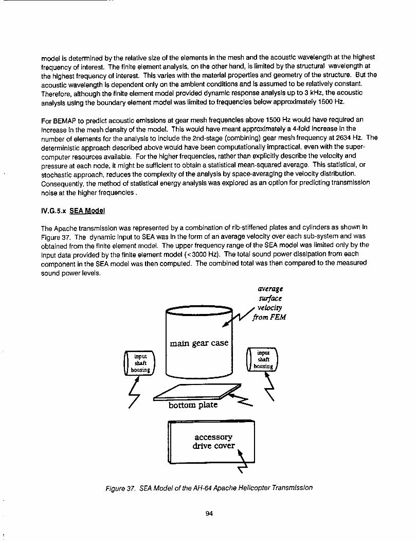
modelisdeterminedbytherelativesizeoftheelementsinthemeshandtheacousticwavelength at the highestfrequency of interest. The finite element analysis, on the other hand, is limited by the structural wavelength atthe highest frequency of Interest. This varies with the material properties and geometry of the structure. But theacoustic wavelength ts dependent only on the ambient conditions and Is assumed to be relatively constant.Therefore, although the finite element model provided dynamic response analysis up to 3 kHz, the acousticanalysis using the boundary element model was limited to frequencies below approximately 1500 Hz.
For BEMAP to predict acoustic emissions at gear mesh frequencies above 1500 Hz would have required anincrease In the mesh density of the model. This would have meant approximately a 4-fold Increase In thenumber of elements for the analysis to include the 2nd-stage (combining) gear mesh frequency at 2634 Hz. The
deterministic approach described above would have been computationally impractical, even with the super-computer resources available. For the higher frequencies, rather than explicitly describe the velocity andpressure at each node, it might be sufficient to obtain a statistical mean-squared average. This statistical, orstochastic approach, reduces the complexity of the analysis by space-averaging the velocity distribution.Consequently, the method of statistical energy analysis was explored as an option for predicting transmissionnoise at the higher frequencies.
IV.G.5.x SEA Model
The Apache transmission was represented by a combination of rib-stiffened plates and cylinders as shown inFigure 37. The dynamic Input to SEA was in the form of an average velocity over each sub-system and wasobtained from the finite element model. The upper frequency range of the SEA model was limited only by the
Input data provided by the finite element model (<3000 Hz). The total sound power dissipation from eachcomponent in the SEA model was then computed. The combined total was then compared to the measuredsound power levels.
I
main gear case
bottom plate
average
surface
_/fro vel°citym FEM
i accessorydrive cover%
Figure 37. SEA Mode/of the AH-64 Apache Helicopter Transmisslon
94

IV.G.6 Experimental Proqram
To develop a methodology for predictlng the noise generated by a rotorcraft transmission, it is necessary tovalidate such a method with a comprehensive vibro-acoustic database from an Isolated transmission. The Intent
is to predict the noise radiating directly from the transmission housing. Therefore, the test transmission was
Installed on a regenerative test stand in an Instrumented test cell. Because of the semi-anechoic nature of thetest environment, it was necessary to measure sound intensity, using spacial averaging techniques, over a
control volume around the gearbox. Noise reflective surfaces in the test cell were covered with 4 inch foam
panels to minimize potential error in the sound intensity measurements. Vibration measurements were obtainedsimultaneously at several location on the casing. The intensity measurements were integrated over the surface
area of the control volume to produce the overall sound power level (PWL). Two transmissions were tested so
that data repeatability could be established. The difference In overall PWL between each transmission waswithin 0.5 dB. The test procedures and data were reported by Hardesty and Hudson [51].
Figure 38 Is a 1/3-octave band plot of the measured sound power levels obtained from the transmission noise
test described in Reference [51]. The acoustic data shown here is for the Apache transmission operating at100% RPM and 100% torque (2828 HP). The 1/3-octave bands containing the gear mesh frequencies and
related harmonics are indicated. A narrow band spectral analysis indicates the presence of an anomalous tone
at 1640 Hz. it is not associated with any of the gear mesh harmonics. Although it was not positively identified, it
is speculated that the tone is the 10th harmonic of the input drive shaft speed of 164 Hz. The highest noise level
is exhibited by the spiral bevel (input) gear In the 5 kHz 1/3-octave band. The accelerometer data also Indicate
that this gear produces the highest vibration levels on the casing. This Is consistent with the NASA/Armyvibration measurements on the OH-58 helicopter transmlss!on [50].
130
120
110
PWL, dB100
re 1012 Watts
90
80.
70.
6o
AH-64 transmission on test stand
anomalous Combining spiraJtone 1stharm. bevel
Pianeia__ Planetary Planetary 1st harm.1st harm. 2nd harm. 3rd harm.
, .¢, ".
630 800 1000 1250 1600 2000 2500 3150 4000 5000
1/3-octave band center frequency, Hz
Figure 38. Measured Sound Power Spectrum
of the Apache Heficopter Transmission
95

Figure39 Is a narrow band spectral plot of the noise measured Inside the Apache helicopter in the pilot cockpit.This data clearly shows that very little of the vibration energy produced by the spiral bevel gear actually gets
transmitted through the airframe and manifests itself as noise In the cockpit. This finding is also consistent with
the acoustic data obtained in a NASA/Army Investigation. Therefore, the discrete tones produced by the
planetary system and the combining gear are of primary concern in the deslgn of quiet transmissions. The data
in Figure 39 also shows no indication of the anomalous tone at 1640 Hz.
Apache Helicopter Cockloit Noise
o
RelativeSPL dB -30
_a-40
-5O
-60
-700
Takeoff at m xim m n
PI P! _ = P=
I(c,_*".2"
P - Planetary gearC Combining gear$8- Spiral Bevel
1 2 3 4 5
Frequency, kHz
Figure 39. Measured Noise Levels in the Cockpitof the Apache Helicopter
IV.G.7 Comparison Between Analysis and Experiment
IV.G.7.i Correlation of Vibration Levels
At all the gearmesh frequencies of interest, the transmission finite element model is used to determine the
vibration levels on the transmission casing. Accelerations at three specific locations on the casing obtained
from analysis are compared to data measured during vibro-acoustic tests on an Apache transmission inTable 21. Boundary conditions used in analysis to obtain these results simulated the test configuration as
closely as possible. Since the transmission was fixed to a solid aluminum plate around the curvic coupling area
during tests, this region of the top cover in the model was grounded. In addition, the input and the output shaftends in the model were grounded through soft and stiff torsional springs to simulate the effect of the peripheral
components.
The results presented in Table 21 show that the model yields vibration levels that are comparable to measured
data at lower frequencies. But at higher frequencles, the deviation between the model and the measurements
becomes significant. The correlation deteriorates more rapidly in the case of the two measurements made atlocation 3.
96

Some general observations can be made based on the comparisons provided in Table 21. The model results
are closer to the measured data at some locations than others. Thus it is difficult to extrapolate from these
results and estimate the error that might be Involved in noise computations, since vibration data from all the
surface grid points are used in such computations. Also, since only the response normal to the surface Is used
in acoustic analysis, large deviations from measured data in the other directions may not necessarily lead to
large deviations In noise estimates. Finally, at higher frequencies, the model tends to overpredict the response
and thus would lead to conservative noise estimates. In light of these conslderations, useful results could still
be obtained from the model in the high frequency range, in spite of the decreased accuracy. The correlations
suggest, however, that the model would produce unacceptable results at very high frequencies (>3000 Hz).
TABLE 21. COMPARISON BETWEEN MEASURED AND PREDICTED VIBRATION LEVELS
(in g's)
Location
No.
2
3
Accelerometer
No.
Test
1
Analysis
Test
2
Analysis
Test
3
Analysis
Test
4
Analysis
Test
5
Analysis
Planetary Harmonics
1st 2nd 3rd 4th
664.7
Combining
Gear
(1st only)
Meshing Frequency (in Hz)
1329.4 1994.1
3.4
14.0
2.0
16.0
11.3
36.0
2658.8
1.8
21.0
4.3
28.0
1.1
2.7
2634.4
2.0
21.8
3.8
12.0
1.8
26.7
2.6
25.2
97
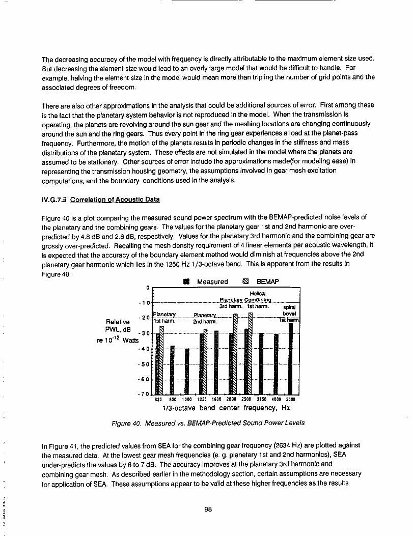
The decreasing accuracy of the model with frequency is directly attributable to the maximum element size used.
But decreasing the element size would lead to an overly large model that would be difficult to handle. For
example, halving the element size in the model would mean more than tripling the number of grid points and the
associated degrees of freedom.
There are also other approximations in the analysis that could be additional sources of error. First among these
is the fact that the planetary system behavior is not reproduced in the model. When the transmission is
operating, the planets are revolving around the sun gear and the meshing locations are changing continuouslyaround the sun and the ring gears. Thus every point in the ring gear experiences a load at the planet-pass
frequency. Furthermore, the motion of the planets results in periodic changes in the stiffness and massdistributions of the planetary system. These effects are not simulated in the model where the planets are
assumed to be stationary. Other sources of error Include the approximations made(for modeling ease) in
representing the transmission housing geometry, the assumptions Involved in gear mesh excitation
computations, and the boundary conditions used in the analysis.
IV.G.7.ii Correlation of Acoustic Data
Figure 40 is a plot comparing the measured sound power spectrum with the BEMAP-predicted noise levels of
the planetary and the combining gears. The values for the planetary gear 1st and 2nd harmonic are over-
predicted by 4.8 dB and 2.6 dB, respectively. Values for the planetary 3rd harmonic and the combining gear aregrossly over-predicted. Recalling the mesh density requirement of 4 linear elements per acoustic wavelength, it
is expected that the accuracy of the boundary element method would diminish at frequencies above the 2nd
planetary gear harmonic which lies in the 1250 Hz 1/3-octave band. This is apparent from the results In
Figure 40.
RelativePWL, dB
re 1012 Watts
In Figure 41, the predicted values from SEA for the combining gear frequency (2634 Hz) are plotted againstthe measured data. At the lowest gear mesh frequencies (e. g. planetary 1st and 2nd harmonics), SEA
under-predicts the values by 6 to 7 dB. The accuracy improves at the planetary 3rd harmonic and
combining gear mesh. As described earlier in the methodology section, certain assumptions are necessary
for application of SEA. These assumptions appear to be valid at these higher frequencies as the results
98

herearegood.Resultsforthespiralbevelgear frequency (4756 Hz) are also shown. However, the
vibration data for this frequency was obtained from the measured accelerometer data since the FE modelwas limited to analysis at frequencies below 3 kHz. The combined result from both the boundary element
method and statistical energy analysis is shown in Figure 42. The results are listed numerically in Table 22.
RelativePWL, dB
re 1012 Watts
o I! Measured [] SEA,
10 r l-lelic_l...........................................................................,.................,_pir_---_" Combining =v.ii
1stharm. . ".':. /1_I rlarm
-20 .................................................. Plarnet;_y" ..............................._lanetary Planetary 3rdharm_ illllst harm. 2ridharm. "..1I [] I I
S30 .........................................................
.!!.....Ii...........................-70 .........
630 100 I000 1250 16002000 2500 3t50 40005000
l/3-0ctave band center.frecluency, Hz
Figure 41. Measured vs. SEA-Predicted Sound Power Levels
[] Measured[] BE_[] SEA
O t Helical
-10 I 1stharm.
Relative"2°_i_i_; _dh_n'C_:_h='n. i'
S_r=Bevel
.._2 Watt'.3o ................... - --re I
1........-50 ...............
-60 ...........
-70 • • • _ . ., t30 I00 1000 1250 11002000 2500 3110 40005000
1/3-octaveband center frequency, Hz
Figure 42. Measured vs. Combined (BEM and SEA)Predicted Sound Power Levels
99

TABLE 22. TRANSMISSION NOISE PREDICTION VALIDATION
(AH-64 Apache helicopter transmission)
Gear Mesh
Harmonic
Planetary: 1st harm
2nd harm
(Unknown) 1
3rd harm
4th harm
Combining: 1 harm ,
Spiral Bevel: 1st harm
Frequency
Hz
664.7
1329.0
1640.0
1994.0
2659.0
2634.0
4756.0
1/3-octaveCenter
Freq,
Hz
63O
1250
1600
200O
2500
5000
Measured
PWL, dB
re 10"12
Watts
99.9
99.6
101.5
99.8
102.72
106.2
Predicted
PWL, dB
re 10"12
Wafts
104.7
102.2
103.5
106.0
DPWL
dB
+4.8
+2.6
+3.7
+3.3
1An anomalous harmonic excitation was observed at 1640 Hz during the AH-64 transmission noise
test. This frequency does not correspond with any of the known gear mesh frequencies of thetransmission or the input drive system of the regenerative test stand.
2Comblnation of planetary 4th harmonic and combining gear 1st harmonic
The sound pressure or sound intensity distribution on the surface of the transmission, computed by BEMAP,can be conveniently plotted on the boundary element model. An example Is shown in Figure 43. The post-
processor used in this case is PDA/PATRAN TM. Plotted here are the surface sound pressure levels at the
planetary gear mesh frequency of 665 Hz. The highest levels are observed in the vicinity of the input shaft andpinion gear housings on both sides, near the accessory gear box (dark shading). There are also some "hot
spots" where high sound pressure levels are radiating from the front face of the gear box. Apparently, theplanetary gear mesh loads are transmitted through the shaft bearings at the planetary and combining gears, andultimately, through the 1st-stage gear housings. A similar sound pressure distribution was observed at the
planetary 2nd harmonic.
The FE/BE model was fine-tuned by adjusting the damping ratio in the finite element model. This was a totalsystem damping ratio distributed over the entire structure (e. g. shafts, housing, etc.). Acoustic power radiatedat the planetary gear mesh frequency was evaluated over a range of damping ratios. Figure 44 shows thesensitivity of the predicted sound power level to the system damping. A damping ratio of 5% critical waschosen as a nominal value for the final predictions. The transmission gears, shafts, and bearings are made ofsteel, and are therefore fairly stiff. But the housing is made of a cast magnesium alloy. Reference [48] (Lazan)shows that test specimens made from such alloys have structural damping ratios as high as 17 percent. Thecombination of a stiff drive train, a housing with relatively high damping, and lubrication in the gears, suggests
that an overall damping ratio of 5% critical (10% structural) Is a reasonable estimate.
100

Figure 43. Surface Noise Contour on Transmission Housingat Planetary Gear Mesh (665 Hz)
15
10-
5-
RelatePWl., dB
o
-5-
Planetary gear mesh, 665 Hz
-10 , I , I , I , I ,0 2 4 6 8 10
system damping ratio, %
Figure 44. Effects of Structural Damping on PredictedGearbox Noise Levels
101

IV.G.8 Description of the MDHC Adv{In_ed Rotor(:reft Transmission
The interior components of ART are illustrated in Figure 45. It Is a 3-stage transmission rated at 5000 HP and
weighs 815 pounds. The 1st-stage consists of two input pinions turning at 20952 rpm, each driving a pair of
face gears with a mesh frequency of 9778 Hz. The 4 face gears drive the 2nd-stage which consists of four spurs
driving a single combining gear with a mesh frequency of 3107 Hz. The combining gear then drives the 3rd-stage. Here, a sun gear drives six high contact ratio (HCR) planetary gears with a mesh frequency of 797 Hz.
This planetary system drives the output shaft at 290 rpm. The key features of the gear design which are
expected to help reduce radiated noise are the split-torque configuration and the HCR planetary gears.
Figure 46 shows the transmission casing which has about 50% more radiating surface than the Apache
transmission. Currently, there Is no added rib-stiffening In the gear casing for noise reduction. The BEMAPanalysis indicated a casing noise radiation efficiency comparable to that of the Apache transmission casing.
The option of caslng modification can be investigated to optimize its design for low noise radiation efficiency.
{ GEAR
RINGGEAR IDLER
GEAR
NOTAR
OUTPUT
FACEGEAR
FACE
GEARSPURGEAR
Figure 45. ART Gear Arrangement
102

Figure 46. ART Outer Casing
IV.G.8.i BaselinQ Transmlsslo,n Noise Level
The estimated noise level for a state-of-the-art 5000 HP transmission was based on measured acoustic trend
data obtained from the 2828 HP Apache helicopter transmission operating over a range of torque settings.
This data is plotted in Figure 47. The measured overall sound power level (OAPWL) for the Apache helicopter
transmission is 110.8 dB re 10-12 Watts at 2828 HP. The trended noise data indicate an increase of 1.2 dB
going from a 2828 HP transmission to 5000 HP. The 5000 HP SOA transmlssion Is expected to produce a 112dB overall sound power level. The ART goal would be 10 dB less, or 102 dB. However, if we disregard the
anomalous tone in the 1600 Hz 1/3-octave band, the measured Apache overall noise level drops by 1.3 dB to
109.5 dB. This approach, in effect, sets an even stricter noise goal for ART. Additionally, as Indicated earlier,
the 1st-stage gear mesh frequencies In both the Apache transmission and ART are beyond the range of the
analytical models. Since it has been well established that the 1st-stage gear mesh is not a major contributor tothe vehicle interior noise levels, the measured noise produced by the spiral-bevel gear In the Apache model is
also disregarded. This again is in the Interest of conservativism in establishing a noise goal for ART. Therefore,the measured noise levels produced by the Apache transmission planetary system and combining gear totals
106.7 dB. Consequently, the estimated state-of-the-art baseline noise level (+ 1.2 dB) becomes 107.9 dB, and
the corresponding noise goal for ART is 97.9 dB (10 dB less). The mesh frequency of the 1st-stage (face gear)
in ART is 9778 Hz, approximately twice that of the spiral-bevel gear in the Apache transmission. This places It
well beyond the speech interference range of the frequency spectrum. The SOA baseline transmission noiselevel is shown in Table 23.
103

120
PWL. dB
re 1 0"12Watts
typical industry trend fromwide range of ITansrrusslonl
115' _. ,- " Projoc'll¢l A,_C_e
j : at _00 HP
_odA_-_i _ _ .112 aS_'itnlmislion not81 _
11o ............................................_ ..............................................................
/i J-10 d8
105 ....... - ...........................
• ,, 102 dB
10¢
2 3 5 7 10
Horsepower x 1000
Figure 47. ART Transmission Noise Goal from Apache TransmissionNoise Trend Data
TABLE 23. ESTIMATED NOISE LEVEL FOR BASELINE TRANSMISSION
Measured Apache transmission noise
(planetary and combining gear mesh
frequencies only)
Baseline 5000 HP (+ 1.2 dB)
106.7
107.9
OAPWL
(dB re 10"12 Watts)
104

IV.G.9 Application of MethodoloQy to ART
IV.G.9.i Finite Element Model
The procedure followed in developing the ART finite element model parallels that used for the Apache
transmission model. As in the case of the Apache model, ART was divided into several components each of
which was modeledseparately. The overall model was obtained by assembling the individual component
models.
Figure 48 depicts the representation used for the internal components. The planet carrier, the ring gear, the
combining gear, and the gearwebs were modeled with quadrilateral and triangular plate elements. The
gearshafts were modeled with one-dimensional bar elements and rigidly tied to the webs. The top, intermediate,
and lower ART casing models are shown in Figures 49, 50, and 51. Plate elements were used in most regions,
combined with solid elements to represent the flanges in some areas. The maximum element size in the model
is about 2.7 inches, which is smaller than the maximum size in the Apache model. It follows that the ART model
can be expected to produce results of comparable accuracy at higher frequencies than the Apache model. This
is essential since the range in which results are required for ART is higher (up to 3200 Hz compared to about
2700 Hz for the Apache).
.F
X y
Figure 48. FEM of ART Internal Components
105

Figure 49. ART Top Cover
Figure 50. ART Intermediate Casing
Techniques used to model the bearings and gearmeshes of the Apache transmission were also used for ART.
The complete model obtained by combining the various components is illustrated in Figure 52. This model
possesses approximately 3600 nodes and 3450 elements. Typical stresses obtained from a static gravity
loading analysis are shown in Figure 53.
106

Figure 51. FEM of ART Lower Casing
ART FEM
Figure 52. Complete FEM of ART
107

ii4"<
_[NGOflHPERSYBNHISESSTRESSES- ZI
451 - A
417 - B
384 - C
350 - D
316 - E
283 - F
249 - G
215 - H
182 - I
148 - J
114 - K
80- L
46-M
13-N
-20 - 0
Figure 53. Stress Contour Plot from Static Gravity Loading (stresses in psi)
IV.G.9.ii Gear Mesh Excitation
Gear mesh excitations for ART were computed using procedures discussed earlier. Only the second and third
stage meshes, consisting of the combining and the planetary gears, were considered in the analysis. Response
to gear mesh excitations were computed at the first four harmonics of the planetary system and the first
harmonic of the second stage mesh. Fundamental frequency of the planetary mesh is 797 Hz, while the
meshing frequency for the combining gear Is 3107 Hz. The first stage face gear meshes were not Included in
the analysis since these occur at a very high frequency (>9000 Hz).
The gear tooth dimensions needed to calculate tooth compliance were obtained from design data. In
computing the transmission error from the compliance data for each mesh, various tooth profile modification
amounts were specified and the excitation harmonics determined. The modification amounts that resulted in
the lowest amplitudes for the harmonics of the transmission error were used in the analysis. These optimum
tooth profile modification data are listed in Table 24 for each mesh. The casing response was obtained with the
resulting excitations at all the frequencies of interest.
108

TABLE 24. LINEAR PROFILE MODIFICATION DATA FOR GEAR TEETH
Gear
Sun
Planet
Ring
2nd Stage Pinion
2nd Stage Gear
Roll Angle at Start of Tooth
Modification (deg)
24.0
26.0
16.9
27.3
27.0
Amount of Modification
at Tip (in.)
0.0008
0.001
0.001
0.00085
0.00085
IV.G.9.iii Boundarv Element Model
Figure 54 shows the boundary element model of the MDHC ART design. It was derived from the finite element
model in a manner similar to that of the Apache transmission and consists of 1754 elements. The geometry of
the ART casing is somewhat simpler than that of the Apache model. Since the ART finite element and boundary
element models were carefully developed with the specific application in mind, they are a better representation
of the actual geometry than those developed for the Apache transmission models.
Figure 54. ART Boundary Element Model
109

IV.G.9.1v SEA Model
For application of statistical energy analysis at the combining gear mesh and the planetary 3rd and 4th
harmonics, ART was represented by a combination of cylindrical shells and flat plates. The average surfacevelocity over each subsystem was obtained from the finite element model in a manner similar to that used for
the Apache transmission. The sound power dissipation from all subsystems were combined to give the totalradiated sound power.
IV.G.10 Discussion of Results
To quantify the predicted noise emissions for ART, it was necessary to establish a correction factor which
represents the error margin associated with the noise prediction methodology. The correction factor wouldthen be applied directly to the ART noise prediction. This necessitated a direct comparison between the noiselevels predicted for the Apache transmission and the corresponding measured values. These comparisons aresummarized in Table 25. Rather than apply corrections to each individual harmonic in the ART evaluation, theerror margin was determined for the combined total noise level. This, as it turns out, is a more conservativeapproach, A total correction factor of -3.6 dB (measured-predicted) was derived for the overall sound powerlevel. This correction factor was applied to the predicted overall sound power level for ART.
TABLE25. TRANSMISSION NOISE PREDICTION ERROR CORRECTION
(AH-64 Apache helicopter transmission)
Gear MeshHarmonic
Planetary: 1st harm
2nd harm
3rd harm
4th harm
1st harm
Frequency
Hz
664.7
1329.0
1994.0
2659.0
2634.0
Octave
Center
Freq,
Hz
500
1,000
2,000
4,000
Measured
PWL, dB
re 10-12
Watts
99.9
99.6
99.8
102.71
Predicted
PWL, dB
re 10-12
Watts
104.7
102.2
103.5
106.01
Combining:
OAPWL 106.7 110.3
1Combination of planetary 4th harmonic and combining gear 1st harmonic.
110

Table 26 summarizes the noise predictions for MDHC's current ART design. The predicted noise levels were
obtained by Implementing the same procedures used in the Apache transmission noise evaluation. When the3.6 dB correction factor from Table 25 Is applied to the predicted value for OAPWL, a total noise reduction of 9.6dB is achieved in the current MDHC ART design, relative to the baseline transmission noise level of 107.9. Thereduction in overall transmission noise level is due prlmarily to a combination of several design features. The
analysis demonstrated that a high contact ratio (CR) between the sun-planet (CR = 2.24) and ring-planet(CR= 2.48) gear meshes provides a significant reduction in the dynamic response of the meshing forces, andsubsequent reduction In noise produced at the planetary gear mesh harmonics. The contact ratios used in theApache transmisslon are 1.5 and 1.67, respectively. Reduced noise levels were also indicated by Increasing thecontact ratio from 1.64 (in the Apache transmission) to 1.7 at the combining gear stage. Another majorcontribution to overall system noise reduction was accomplished by optimizing the tooth profile modification atthe planetary and combining gear stages. The finite element analysis provided a means to evaluate the effectsof such modifications on the system dynamic response and noise. Finally, mass stiffening of variouscomponents including the ring gear web, sun gear shaft, and the gear box caslng, Indicated further potential for
optimizing the ART design for low acoustlc emissions. Planetary gear phasing was also employed as a noisereduction feature in the ART design. However, this Is considered a state-of-the-art noise control feature which
already exists in the baseline transmission design.
TABLE 26. ART NOISE PREDICTIONS
Gear Mesh
Harmonic
Planetary: 1st harm
2nd harm
3rd harm
4th harm
1 harm
Frequency
Hz
797.0
1594.0
2391.0
3188.0
3107.0
Predicted PWL, dB
re 10"12
Watts
98.0 (BEM)
95.9 (BEM)
90.0 (SEA)
84.0 (SEA)
96.0 (SEA)Combining:
OAPWL 101.9 98.3
Plus
Correction
(-3.6 dB)
IV.G.11 Summary of Results
The acoustics assessment of the MDHC Advanced Rotorcraft Transmission (ART) is based on validated
analytical techniques. The methodology employs the use of finite element methods to determine the dynamicresponse of the gear box casing. This excitation of the casing, due to the gear meshing forces was used forcalculating the case-radiated noise. The acoustic calculations were accomplished by a combination of adeterministic approach, based on the boundary element method, and a stochastic approach, based onstatistical energy analysis (SEA). It was necessary to employ both of these methods to evaluate the gear meshharmonics in the frequency range of interest. The combined dynamic and acoustic analyses were validated by
111
application to an existing AH-64A transmission and comparing the results to a vibro-acoustlc data baseobtained during a comprehensive sound intensity survey of the transmission operating on a regenerative teststand. The validation provided a high degree of confidence in both the dynamic and acoustic models used inthe ART noise assessment. The validated methodology was then applied to the MDHC ART design. Majornolse reduction features were Incorporated In the design which were evaluated by using advanced dynamic andacoustic prediction methodologies. These features can not be evaluated using conventional analyticaltechniques. Results indicate an overall noise reduction of 9.6 dB relative to a current state-of-the-arttransmission rated at the same horsepower. Although this falls short of the program goal of 10 dB noise
reduction, the analytical procedures allow for "design-to-noise" capability. Preliminary parametric studiesindicate a strong potential for optimizing the ART design to achieve maximum noise reduction withoutexceeding the weight goal.
112

V. MISSION EFFECTIVENESS
The mission effectiveness analysis of a Future Attack Air Vehicle (FAAV) which uses the Advanced Rotorcraft
Transmission (ART) is presented herein.
The FAAV is visualized by MDHC as a twenty-first century air vehicle that is versatile, highly maneuverable,
serviceable and stealthy. It wgl be capable of air-to-air (ATA), air-to-ground, anti-armor, and special electronic
mission aircraft (SEMA) missions conducted worldwide, day or night, In all weather conditions.
Several key performance parameters of the FAAV are evaluated herein to determine the benefits that would be
derived from the performance characteristics of the selected ART configuration. This analysis focuses on the
system, not just the transmission, and it considers the synergism of the transmission performance on the FAAV
as a total system.
This section is segmented into three subsections:
• Mission Analysis
• Reliability
° Life-Cycle Costs
Mission Analysis is an assessment of lethality and survivability of the aircraft. As part of the ART program, an
evaluation of how the improved transmission impacted misslon effectiveness was studied. Although the
changes being considered affected all areas of mission performance, past experience indicated that the most
demanding area would be a close-in, air-to-air engagement. Accordingly, the alr-to-air engagement was the
focus of this analysis.
FAAV Reliability will be much improved over current generation aircraft. The amount of Improvement is
estimated by trending previous and current design rellabilities. Assuming the FAAV is a next-generation design,
the trend is to double reliability requirements every generation. This results in an FAAV system reliability of 18
hours with mission reliability Increasing from 22 to 75 hours.
Life Cycle Costs (LCC) estimates were made for three configurations: baseline FAAV, ART Improved FAAV, and
optimized FAAV with ART. This report contains the estimates and a discussion of the techniques and
assumptions used to make those estimates. The LCC estimate is reflective of the technological advances
(composites and integrated mission equipment) and operating conditions inherent in designing and fielding an
aircraft in the next century.
V.A MISSION ANALYSIS
As part of the Advanced Rotorcraft Transmission (ART) project, there was a requirement to evaluate the effect
on mission effectiveness of using an advanced rotorcraft transmission of lighter weight, variable RPM, andgreater reliability in a conceptual Future Attack Air Vehicle (FAAV). The proposed design changes affect the
aircraft's ability to perform its mission, and can be translated into a comparison of the lethality and survivability
of FAAV equipped with the candidate transmission designs. Although the changes being considered affect all
113

areasofmissionperformance,past experience indicated that the most demanding area would be a close-in air-to-air engagement. Accordingly, the air-to-air engagement was the focus of the analysis.
V.B APPROACH
The primary changes incorporated, or considered, inthe candidate ART designs were the following:
= Weight reduction of 622 Ib compared to an upgraded Apache-type transmission
• 5000 horsepower capability
• Increase in mean-time-between-removals (MTBR) to 6200 + hours
Q Ability to temporarily increase rotor RPM to 120 percent.
The aircraft selected to evaluate the ART was a conceptual FAAV, modeled as a follow-on Apache design, withupgraded capabilities. Specifically, the FAAV Included:
• Engines of 3000 HP each (6000 HP total)• 5-bladed rotor system with 25-inch blade chord
• NOTAR anti-torque system
The baseline aircraft used for comparison was the FAAV mentioned above, equipped with an upgraded Apache-type transmission. This configuration is referred to as the baseline FAAV in this section. The second
configuration referenced in this section is the ART improved FAAV. This is the same FAAV aircraft, modeled asa follow-on Apache design, equipped with the 5000 HP ART transmission. The third configuration is referred to
as the optimized FAAV withART. This configuration assumes that the a_rcraftwas designed from the ground upwith the ART transmission. Operation of the main rotor at 120% RPM is assumed for this configuration to
evaluate potential mission analysis and cost benefits.
The scenario used was an air-to-air engagement between the three FAAV aircraft configurations and selectedthreat helicopters. The basic engagement was between two Blue aircraft and four Red aircraft, to ensure the
Blue aircraft were properly stressed.
V.C THREATS
The threat was represented by the MI-28 "HAVOC," and the KA-35 "HOKUM."
V.D ENGAGEMENT MODEL
The Air Land Engagement Simulation (ALES) was used to evaluate the air-to-air encounters. The few-on-few
ALES model simulates the performance of the aircraft and their weapons systems, and evaluates the outcome.
A total of ten combinations of initial headings for the aircraft were evaluated for each test case. The aircraft
configurations and weapons toads that were modeted are given In Tabte 27.
114
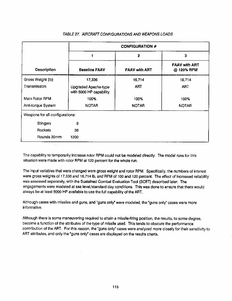
TABLE 27. AIRCRAFT CONFIGURATIONS AND WEAPONS LOADS
Description
Gross Weight (Ib)
Transmlsslon
Main Rotor RPM
Anti-torque System
CONFIGURATION #
1 2 3
Baseline FAAV FAAV with ARTFAAV with ART
@ 120% RPM
17,336
Upgraded Apache-typewith 5000 HP capability
100%
NOTAR
16,714
ART
100%
NOTAR
16,714
ART
100%
NOTAR
Weapons for all configurations:
Stingers 8
Rockets 38
Rounds 30mm 1200
The capability to temporarily Increase rotor RPM could not be modeled directly. The model runs for thissituation were made with rotor RPM at 120 percent for the whole run.
The Input variables that were changed were gross weight and rotor RPM. Specifically, the numbers of interest
were gross weights of 17,336 and 16,714 Ib, and RPM of 100 and 120 percent. The effect of Increased reliability
was assessed separately, with the Sustained Combat Evaluation Tool (SCET) described later. Theengagements were modeled at sea level/standard day conditionso This was done to ensure that there would
always be at least 5000 HP available to use the full capability of the ART.
Although cases with missiles and guns, and "guns only"were modeled, the "guns only" cases were moreinformative.
Although there is some maneuvering required to attain a missile-flringposition, the results, to some degree,become a function of the attributes of the type of missile used. This tends to obscure the performance
contribution of the ART. For this reason, the "guns only" cases were analyzed more closely for their sensitivity toART attributes, and only the "guns only" cases are displayed on the results charts.
115

As indicated in Table 27, the only differences between the configurations were gross weight and rotor RPM.
three aircraft configurations were run against both types of threat helicopter. The measures of effectivenesswere:
All
Lth_ - Threat helicopters destroyed
Survivability - Blue helicopters surviving
Exchanae Ratio - Red losses divided by Blue losses
FEirlngOpportunities - Blue firing opportunities for a given run (equal to the number of bullets expended
by Blue)
En_agem?nt Time - The total time required to complete the engagement.
As indicated, the "firing opportunities" represents the number of rounds fired by the guns of the Blue aircraft.Since a round is not fired unless the targeting constraints are met, the firing of each round was considered a
firing opportunity.
The total engagement time is an average of all engagement times for a given set of clrcumstances, and is ameasure of the efficiency of the weapon system.
The FAAV aircraft were also evaluated with the SCET model. This Is a program that calculates the Impact of
combat losses, combat availability, resupply times, and initial force levels on combat sustainment. This toolevaluates the mission impact of the increased availability of the ART, in addition to any increased combateffectiveness.
V.E RESULTS AND CONCLUSIONS
V.E.1
The ALES program uses an imbedded helicopter performance model called the Maneuver Criteria EvaluationProgram (MCEP). Prior to running the ALES program, the necessary MCEP parameters must be generated for
the specific aircraft conditions of interest. These parameters are then used by MCEP during the ALES runs to
provide performance information for the ALES model. Three MCEP runs were completed. The first two were at100 percent rotor RPM with different gross weights. The third was at 120 percent rotor RPM, at the lighter of the
gross weights. The speed-power polar plots generated during these runs provided interesting insight into the
effects of Increasing rotor RPM.
116

Figure55showsacomparisonof the three cases, the two 100% RPM cases and the lighter gross weight at
120% RPM. From Figure 55 it can be seen that at 160 kts, there are still approximately 1,300 excess
horsepower available for the 100% case, Configuration 2. However, the aircraft is transmission limited (5000
HP) at approximately 150 kts for the 120% case, Configuration 3. An investigation of the associated MCEPparameters indicated the cause. The combination of increased rotor RPM and Increasing forward speed caused
the main rotor tip speed to enter the trans-sonic range. At Mach numbers above 0.9, the compressibility effectsbegin to dominate power requirements. For example, at 100% RPM and 160 kts, the power required to
overcome compressibility effects is 555 HP. For the same airspeed at 120% rotor RPM, 2540 HP is required toovercome compressibility effects.
This situation obviously affected the amount of excess power available (which is directly related to vertical rate
of climb (VROC), for the 120% RPM case. In the extensive maneuvering of air-to-air engagements, VROC is very
important. The results of the ALES runs generally verified the Importance of excess power In air-to-airengagements. The Configuration 2 (16,714 Ib, 100% RPM) cases were consistently more effective than the
other two cases. The reduced weight provided additional excess power that translated to additional VROC. As
shown in Figure 56, Configuration 2 produced more Blue survivors, resulting In consistently higher exchange
ratios (17 to 22% higher than Configuration 1, and 52 to 73% higher than Configuration 3).
5OOO
45OO
/
£,"I-
o¢l
I--
4000
3500
3OOO
25O0
2OOO
1500
\\
_% •
_ _ ._,..... I "_
/i
/7-f FAAV 17/--
/ : (!) ,r-
r./ / /
/,,/" /'F_,vwrrH ART ]--/" t_%;'RPM (2) ;_-
[
lOOOo 20 40 60 80 100 120 140 160
Velocity (Knots)
Figure 55. Speed Power Polar Comparison Apache FAAV
(Configurations 1, 2, and 3)
117

<LLIG_I
D
0I
i! iliiii!ii i i,i¸ ¸
1.0 0 1.0 0 I_0 o _ 0¢0 oO ¢xl 0,,I ",- ",--
(03S) S31AIIIIN3_39V_N3 3_VW3AV
<wm7"I-00><7-
L_ O LO O I._ O I._ OCO CO 0_ O_ ",-- ,-
(O3S) S31AIII IN31AI3OVE)N3 39VW3AV
w
ZGOi.urr
I1.
OOozLLI
p--<11tCC-1-I--:5Dx,"oI
O O O O O OL_ O If) O0_ O_ ',-- "I-
IN3_39V_N3/03WI3 SONO0W
LLICC7-I--OO><7-
0 0 0 0 0 0
04 04 ',-- ',-
IN3_3DVON3/O3WI3 SONOOW
rrw
LU 0><
I-<IIIm-rI--_5D
o7-
cOO _ O _ O _ O
$3S$073_78iS3SS0703W
<wOZI
o0
7"
0
O0 ::::--:-:--::-.-:---:.--
O : j:i ::::: ::
Iiii!ii_!i!i!i!i!i!iii!iiiiiiiiiii!ii_iiii:iiiiiiii_iiiiiiii_i!i!__i
09 |.i_,> •........:-......_!.........._'L,f:" *._o "-':_ _ ...._, ..
_0 O If) O u0 O
$3SS07 3_78/$3SS0-1 03_1
n _.rr r'r
O #_- o 0_
rr _17"
LLI < <(9 T 7"Z I-- I--
7-> >
0 > <×n II
H
118

Configuration 3, though lighter than Configuration 1, suffered a serious lack of excess power, due to the
compressibility power requirements discussed earlier. This 120% RPM case was consistently less effective than
either of the other two (23 to 42% lower exchange ratio). The above statements hold for engagements againstboth threat helicopters. An analysis of firing opportunities and total engagement time indicated the
Configuration 2 aircraft required fewer rounds, and less time to complete the engagement, demonstratingslightly greater efficiency and significantly better effectiveness.
The evaluations with the SCET tool indicated that the combination of increased reliability and better exchange
ratio of the ART equipped FAR (100% RPM), resulted in 12.80% Improvement in the capability to sustain a givenlevel of combat operations.
These results are significant in that they show the relative effectiveness of the different versions of the FAAV
against a given threat helicopter. The reported numbers of Blue and Red kills are not predictions of the resultsof actual combat, they are analytical results dependent on many assumptions and modelling variables. The
performance of the threat aircraft is based on unvalidated individual performance models. In the case of the
Hokum, this model is based on "best estimates of performance." Although comparisons of the different FAAV
aircraft configurations against the same threat are valid, it is not valid to compare results of a given FAAV variantagainst _ threats.
V.E.2 Conclusions
• The use of the ART transmission (100% case) produces a 17 to 22% increase in the loss exchange ratio ofRed losses to Blue losses, compared to the baseline FAAV.
The ability to sustain rotor RPM at 120% provided no advantages, and, due to the substantial additional
power required, resulted in a 24 to 42% decrease in loss exchange ratio when compared to the 100% RPM
case, at the same gross weight. Use of varying RPM during engagement was not modeled.
• In all cases, the FAAV with ART, 100% RPM case was more effective than the other two configurations.
V.F RELIABILITY
V.F.1 FAAV Mi_sion Reliability
Because the FAAV Is a next-generation design, the trend is to double reliability requirements every generation
(see Figure 57). This analysis is based on substituting an ART for a AH-64A transmission. The reliabilityequation for this substitution is:
1/(ART MTBF) = SUM 1/Standard MTBF's- 1/AH-64A Transmission Mission MTBF
+ 1/ART Mission MTBF
119

100
50
3O
20
-'-_ 10t_
E 5
m :3
2
j J' F V
(Projected)/
Apache(AAH)
Design
Generation
Figure 57. Trend in Military Helicopter System Reliability
The design features which enhance transmission reliability, improving MTBR from 1500 hours (2) to 5000 hours,
will have a proportional improvement on mission (and system) reliability.*
ART Mission MTBF = ART MTBF/AH-64A Transmission MTBR*AH-64A Transmission Mission MTBF
Using the current actual mission reliability of the AH-64A, transmission of 354 hours MTBF ([53]:
ART Mission MTBF = 500/1500"354 = 1180 hours
Using the current actual mission MTBF of the AH-64A of 22 hours [53]:
ART-AH-64A Mission MTBF = 1/(1/22 - 1/354 + 1/1180) = 23 hours
For an Apache equipped with an ART, mission reliability will increase 4.5% from 22 to 23 hours MTBF.
For the FAAV with the projected mission reliability of 88 hours:
ART-FAAV Mission MTBF = 1/(1/88-1/354 + 1/1180) = 107 hours
For an FAAV equipped with an ART, mission reliability will benefit 22% from 88 to 107 hours MTBF.
*Mission reliability accounts for any failure in the system which causes a mission abort. This includes chip
detector lights coming on (whether Justified by a transmlssion problem or not) and even perceived failures suchas excessive vibration. System reliability accounts for any system failures.
120

V.F.2 FAAV System R_liability
The current system reliability of the Apache drive system is 61.6 hours [53]. ART-related improvements will
increase this number proportional to the MTBR improvement:
ART System MTBF = 5000/1500"61.6 = 205
Substituting the ART for conventional transmission shows the impact to the FAAV:
ART-FAAV MTBF = 1/(1/18-1/61.6 + 1/205) = 22.6
An FAAV equipped with an ART will benefit by an increase in system reliability of 25.5% from 18 to 22.6 hours.Consequently, aircraft availability will also Improve.
V.G LIFE CYCLE COSTS
An LCC estimate was completed for the baseline FAAV, ART improved FAAV, and optimized FAAV with ART.
V.G.1 Methodology
The LCC estimate is broken down Into three phases: Investment, Research and Development, and Operatingand Support.
Parametric and analogous cost estimating techniques were the primary methods employed in determining the
LCC impacts associated with the Advanced Rotorcraft Transmission (ART) and the Future Attack Air Vehicle(FAAV).
Parametric estimating is accomplished by correlating design parameters to historical costs through a regressionanalysis that describes the relationship of cost to those parameters.
The GE PRICE (Parametric Review of Information for Costing and Evaluation) hardware model was employed in
estimating airframe and mission equlpment mechanical and electrical (development and production) costs.
Technological advances In mission equipment resulted in the followlng adjustments to the PRICE model:
• Reduced risk due to commonality of modules between weapon systems such as the Advanced TacticalFighter and FAAV
• Reduced integration costs, resultlng from a fully Integrated system which allows for the elimlnation of
special test equipment currently required to perform system checkout.
Analogous estimating Is based on the known cost of a similar Item In a prior system. Adjustments are made to
the known costs to account for differences in relative complexities of the performance, design, and operationalcharacteristics of the compared Items. The analogous systems used for comparison were the AH-64A, AH-1T,
and the Advanced Composite Airframe Program (ACAP). The lines of code for airbome and ground system
software were based on similarities to the F-15 and Advanced Tactical Fighter Programs using the Ada software
121

language. The estimate and a discussion of the techniques and assumptions used to make those estimates are
included in the following paragraphs.
V.G.2 System Description
The estimate for each configuration was broken down to the subsystem level. This was necessary to show the
impact of Incorporating the ART into the FAAV aircraft.
Subsystem Breakdown:
• Structure • Hydraulic/Pneumatic• Armor • Electrical
• LandlngGear • Fuel
• Propulsion • Environmental Control System
• Rotor • Furnishings and Equlpment• Drive • Crewstation
• Flight Control • Mission Equipment
V.G.3 Acquisition Cost Estimates_ (Ground Rules and Assumptions)
The following set of ground rules and assumptions wereused to develop the acquisition cost for the baseline
F,_V, ART improved FAAV, and optimized FAAV with ART air vehicle configurations.
Economic Base Year. All cost data and estimates are reported in base year 1988 dollars.
Develol_ment Quantity. Nine prototype air vehicles are assumed.
Production Quantity. This estimate assumes that 600 aircraft will be procured for each configuration.
Schedule. The acquisition schedule as provided:
DEM/VAL
Full-Scale Development
Prod uction
Start First Adlcle Completion
Jan/2000 Dec/2003
Jan/2003 Dec/2004 Dec/2006
Jan/2005 Dec/2006 Dec/2013
Production Buildup. The production rate buildup schedule based on an evaluation of current programs:
FY06 FY07 FY08 FY09 FY10 FY11 FY12 FY13
12 24 48 72 120 120 120 84
122

Software. Three million lines of code will be developed with the programmer averaging 2.5 manhours per line
of code based on an evaluation by the software development organization.
COSt Exclu_tion_t. The following acquisition elements were not considered in this estimate:
• Retrofit
• Industrial Facilities
• Operational Site Activation
Developrne_nt Methodoloay. Research and Development (R&D) cost is defined, in general, to be the sum of allcosts resulting from applied research engineering design, analysis, development, test, evaluation and managing
development efforts related to a specific material system. The Department of the Army Pamphlet 11-2,
"Research and Development Cost Guide for Army Material Systems," addresses the following cost elements:
1.0 Research and Development Cost
1.01 Development Engineering
1.02 Producibility Engineering and Planning
1.03 Tooling
1.04 Prototype Manufacturing
1.05 Data
1.06 System Test and Evaluation
1.07 System/Project Management
1.08 Training
1.09 Facilities
1.10 Other
Parametric and analogous cost estimating techniques were used to drive the total aircraft R&D cost estimates
shown in Table 28. The range from low to high reflects uncertainty In the estimate which is typical during the
conceptual phase of the program. The GE PRICE H-Model was the primary estimating tool. Analogies to AH-64A, AH-1T, and ACAP were used to develop the subsystem manufacturing complexities which are an integralpart of the PRICE estimating process.
Cost Estimating Relationships (CER's) developed from in-house sources were used In conjunction with the
PRICE H output to develop the complete estimate.
123

TABLE28. TOTAL R&D
I Baseline
TotaIR D 2000M-,i247MNOTE:
ART Improved Optimized FAAVwith ART
Costs in millions of dollars (M)
The transmission/drive system R&D estimates were derived using the same approach as the total aircraft. Thedevelopment cost for each configuration Is referenced inTable 29.
TABLE 29. TRANSMISSION R&D ESTIMATE
Total R&D
Baseline ART ImprovedFAAV FAAV
$52.2M - $62.5M $43.2M - $51.8M
Optimized FAAVwith ART
$43.2M - $51.8M
NOTE: Costs in millions of dollars (M)
Production M(tthodoloav. Production (Investment) cost is defined, in general, to be the sum of all costs
resulting from the production and introduction of the material system into the Army's operational inventory. The
Department of the Army Pamphlet 11-3, "Investment Cost Guide for Army Material Systems," addresses the
following cost elements:
2.0 investment Cost
2.01 Non-Recurring Investment
2.02 Production
2.03 Engineering Changes
2.04 System Test and Evaluation
2.05 Data
2.06 System/Project Management
2.07 Operational Side Activation
2.08 Training
2.09 Initial Spares and Repair Parts
2.10 Transportation
2.11 Other
The PRICE H files used in the development estimate were retained for use In creating the air vehicle production
estimate. Table 30 depicts the total investment cost for each configuration.
124

The Advanced Rotorcraft Transmission (ART) recurring production costs were derived based on AH-64A data.
The data was provided via the Material Pricing Section, l.e., purchase order data. The systems and theirrespective costs are listed in Table 30. The systems, where sufficientdata was available, were fitted to a curve
and the appropriate sloes and first unit cost determined.
The objective is to project a baseline transmission cost based on the present Apache transmission. The
baseline transmlssion has a power requirement of 5000 HP.
TABLE 30. INVESTMENT
Investment
Baseline ART Improved Optimized FAAVFAAV FAAV with ART
$9582M - $11,641 M $9487M - $11,525M $9400M - $11,418M
NOTE: Costs in millions of dollars (M)
Two approaches were taken in determining the cost of the baseline transmission. Approach one, makes use of
a study described in Reference [54]. The Drive System's cost estimating relationships (CER's) provided
recurring production cost as a function of weight and quantity. Adjustment factors were derived based on AH-
64A historical data and applied to the algorithms to compensate for up-to-date technology.
The second approach used the GE PRICE H parametric hardware model. Based on the average unit cost of the
first four lots of the AH-64A system, the model was adjusted and complexity factors derived, characteristic to
each individual system. These factors, along with the system weights, were Input into the model and new costsderived.
The results of the two approaches, along with the weights and costs of the McDonnell Douglas Helicopter
Company (MDHC) AH-64A and the MDHC Light Helicopter 500E model, were fitted to a curve by employing
techniques of linear regression. The results yielded an algorithm that estimates transmission cost as a function
of weight. The results of this analysis are shown in Table 31.
TABLE 31. ART RECURRING PRODUCTION COST
i 1,792-1b ]
Recurring Production
NOTE:
1,350-1bART
$420K
Costs shown in thousands of dollars (K) and includes drive system(shafts, couplings)
125

V.G.40oeratinaand Support Cost Estimate
The following set of ground rules and assumptions were used to develop the O&S cost for the baseline FAAV,ART Improved FAAV and FAAV with ART air vehicle configuratlon.
Economic Base Year. All data and estimates are reported in economic base year 1988 dollars.
Operational Scenario. An operating scenario of 420 flight hours per year for 25 years was used based ondirection from NASA.
Maintenance Concept. Two level maintenance (Aviation Unit and Depot) concept was assumed.
Exqlusions. The following elements of cost were excluded from the estimate:
• Other direct support operations
• Unit training
• Transportation• Transients, patients, and prisoners
• Medical support
• Training devices• Software maintenance
_d Support Methodoloqv
Operating and Support (O&S) cost is defined in general to be the sum of all costs resulting from the operation,maintenance and support of the weapon system after it ls accepted into the Army Inventory. The Department ofthe Army Pamphlet 11-4, "Operating and Support Guide for Army Material Systems," addresses the followingcost elements:
3.0 Operating and Support Cost
3.01 Military Personnel3.02 Consumption
3.03 Depot Maintenance3.04 Modifications, Material
3.05 Other Direct Support3.06 Indirect Support
The O&S costs shown In Table 32 were generated using the Quick Look II model. The in-house model is based
on CER's developed through the AVSCOM Maintenance Operating and Support (AMOS) cost mode! and AH-
64A historical data. The Quick Look II model is used to calculate subsystem O&S cost as a function of unit cost
and Reliability/Maintainability (R&M) characteristics of the helicopter.
126

TABLE 32. O&S COST
Total O&S
Baseline ART Improved
FAAV FAAV
$21,058M - $22,824M $20,970M - $22,715M
NOTE: Costs in millions of dollars.
Optimized FAAV
$20,892M - $22,621M
The FAAV aircraft will have lower operating costs than the current generation of helicopters based on the
following: slgnificant increases in reliability common module architecture, reduction in false failures, reduction
in line replaceable units, isolation of failure through self-diagnostics, and standardization of airframe
manufacturing components. Further Improvements are probable as technological advances are incorporated
into the system.
Direct Operating CoFt M_thodoloay
Direct Operating Cost (DOC) is a subelement of O&S cost and consists of the following cost elements:
3.012
3.021
3.022
3.031
3.032
Direct Maintenance
Replenishment Spares
Petroleum, Oil and Lubricants
Depot Labor
Depot Material
The Quick Look II files used in the O&S estimate were retained for use in creating the DOC estimate. The
difference in direct operating cost shown In Table 33 is attributed to Incorporation of the ART into the air vehicle
configurations. The mean time between removal for the ART is 5000 hours versus 1,500 hours for the AH-64A
transmission. This results in a DOC saving for the transmission of approximately 33 percent.
TABLE 33. DOC
Direct Operating Cost
Transmission (only)
Baseline
FAAV
$1,476 - 1,807
$66 - 79
ART Improved
FAAV
$1,460 - 1,787
$44 - 53
Optimized FAAV
with ART
$1,448- 1,772
$44-53
NOTE: Costs shown in dollars per flight hour.
127

V.H CON(_LUSION$
Inherently, a reduction in empty weight of an aircraft enables improvements in most areas of performance.
Relative to the Baseline FAAV, the FAAV with ART offers a choice of added range, ordnance payload, and
improved agility, which is critical in the air-to-air combat environment. Mission Analysis shows that the FAAV
with ART produces a 17 to 22 percent Improvement in the loss exchange ratio (Red losses to Blue losses) when
compared to the baseline FAAV.
Reliability Is improved as well. The FAAV with ART offers much Improved mission reliability with a 22 percent
increase in MTBF (88 hours for FAAV baseline vs. 107 hours for FAAV with ART). System reliability Increased
25.5% in MTBF (18 hours vs. 22.6 hours). Significant decreases in the estimated life cycle costs are as shown in
Table 34.
TABLE 34. WEIGHT/LIFE CYCLE COST COMPARISON
• Transmission weight, Ib
• Aircraft empty weight, Ib
• Aircraft gross weight, Ib
• Aircraft development cost, $ per unit
• Transmission acquisition cost, $ per unit
• Aircraft acquisition cost, $ per unit
• Transmission direct operating cost,
$ per flight hour per unit
• Aircraft direct operating cost, $ per flight
hour per unit
• Transmission fleet life cycle cost, total $
• Aircraft fleet life cycle cost, total $
Baseline
FAAV
1792
10,391
17,336
3.33M - 3.74M
0.64M - 0.77M
19.30M - 23.15M
66 - 79
1,476 - 1,807
800M - 960M
32.64B - 36.71B
ART ImprovedFAAV
1170
9769
16,827
3.31M - 3.71M
0.49M - 0.59M
19.12M - 22.92M
44 - 53
1,460 - t,787
571M - 688M
32.44B - 36.47B
Optimized FAAV
with ART
1170
9769
16,600
3.28M - 3.68M
0.49M - 0.59M
18.94M - 22.71M
44 - 53
1,448- 1,772
571M - 688M
32.26B - 36o25B
NOTE: Included list of assumptions. Also, run at least one case where:
number of aircraft = 600
life cycle period = 25 years
annual utilization = 420 flight hours
128

Vl. MATERIAL CHARACTERIZATION TESTS
VI.A INTRODUCTION
Five near-net forged gear materials and three transmission housing materials were tested as part of the ART
program. The gear materials tested were X53 Pyroware, CBS 600, M50NIL, AISI 9310 and M300. The testsperformed for these were gear tooth scoring tests, single tooth bending tests, Charpy Impact energy tests andcompact tenslon fracture toughness tests. The housing materials tested were C355T7 alumlnum, WE43
Magnesium, and ZE41A magnesium alloys. Tensile tests and compact tenslon fracture toughness tests wereperformed for these. The tests, gear materials, AMS specifications and test quantities are summarized in thefollowing tables.
Tooth Scoring Tests, Single Tooth Bending Fatigue Tests, end Chargv Iml0act EnergvTests-GearMaterials
These tests were performed on specimens fabricated from five different steels as tabulated.
Number of Tests
Material S_ec. Tooth $_oring Tooth Bending ha_C_.b.p_r.p_y
M50NIL 6278 70 20 12
X53 Pyro. 6308 72 20 12
CBS 600 6255 6 12 12
AISI 9310 6265 96 24 12
300M 6514 6 12 12
Fracture Tqughness Tests - Gear and Housing Materials
These tests were performed on specimens fabricated from two magnesium alloys, one aluminum alloy, and twosteel alloys, as tabulated.
Material SDec. Heat Treatment No. of Tests
WE43 N/A Solution Heat Treat 7
ZE41A 4439A Solution Heat Treat 7
C355T7 4215 Solution Heat Treat 6
M50 NIL 6278 Pseudocarburized/Hardened 6
X53 Pyro. 6308 Pseudocarburlzed/Hardened 7
129

T_nsile Tests - Housing Materials
These tests were performed on specimens fabricated from two magnesium alloys and one aluminum alloy astabulated.
M_teri_l _ Heat Treatment NO. 9f Tests
WE43 N/A Solution Heat Treat 24
ZE4tA 4439A Solution Heat Treat 24
C355T7 4215 Solution Heat Treat 24
The selected gear material tests were chosen to allow determination of the relative resistance to tooth scoring,relative bending strength, impact toughness and fracture toughness of the five materials. Near-net forged test
gears were employed in the single tooth bending and scoring tests to determine if any additional benefits couldbe derived from gears produced using the near-net-shape forglng process. The AISI 9310 and M300 steels wereintended as baseline gear materials for use in comparison with the high-hot-hardness X53, CBS 600 and M50NIL
steels and with existing test data.
The tests of the three housing materials were chosen to determine Impact toughness and tensile strength of thematerials. The ZE41A magnesium served as a baseline for comparison with the more advanced WE43
magnesium and C355T7 alumlnum alloys.
VI.B TEST pROGRAMS
VI.B.1 Gear Tooth Scoring Tests
VI.B.l.i Intr0du_tion
The objective of the tooth scoring tests was to compare the relative scoring resistance of near net forged gearsmade from various advanced gear materials. Tests were run at McDonnell Douglas Helicopter Company on 252
specimens consisting of X53 Pyroware, CBS 600, M50NIL, AISI 9310 and M300 gear materials. The test rigcapabilities and test operating conditions were selected to assure that tooth scoring precipitated In all testspecimens. Test conditions were monitored and recorded for each test run, and operating parameters weremeasured with calibrated instrumentation. Following the tests, comparisons made from failure data determined
the ranking of the materials in terms of resistance to scoring. The flash temperature index and probability of
scoring were also determined from the test data for the materials. Recommended design operatingtemperatures were then determined for the materials based on mean value, one sigma and two sigma standardof deviation of the test data.
VI.B.l.ii Test Article Description
Five gear materials consisting of two baseline gear steels and three high-hot-hardness gear steels were selectedfor the tooth scoring tests. AISI 9310 and M300 served as the baseline steels for the tests, while X53 Pyroware,
CBS 600 and M50NIL gear steels were tested as high-hot-hardness candidates for selection in the advanced
130

rotorcraft transmission. The gear materials and test quantities used in the tooth scorlng tests are Identified asfollows:
Part AMS Heat Make No. of
Numl_qr Material _ Treatment From Test_
42499-21-1 M50NIL 6278 Carburlzed and 42499-21-6 70Hardened Forglng
42499-22-1 M50NIL 6278 Carburized and 42499-21-6
Hardened Forging
42499-21-2 X53 Pyro 6308 Carburized and 42499-21-7 72Hardened Forging
42499-22-2 X53 Pyro 6308 Carburized and 42499-22-7Hardened Forging
42499-21-3 CBS 600 6255 Carburized and 42499-21-8 6
Hardened Forglng
42499-22-3 CBS 600 6255 Carburlzed and 42499-22-8
Hardened Forging
42499-21-4 AISI 9310 6265 Carburized and 42499-21-9 96
Hardened Forging
42499-22-4 AISI 9310 6265 Carburized and 42499-22-9
Hardened Forging
42499-21-5 300M 6514 Through 42499-21-10 6.Hardened Forging
42499-22-5 300M 6514 Through 42499-22-10Hardened Forging
The test gears were rough-formed using the near-net forging process. This process was selected because ithas the potential for increasing gear fatigue life and improving the endurance limit. The process also makes
more efficient use of raw materials and greatly reduces or even eliminates the need for secondary machining,depending on the quality class of gear required. The five near-net forged materials were produced by The EatonCorporation inWilloughby Hills, Ohio.
The material certificates and chemical compositions are outlined in Tables 35 and 36. All heat treatmentoperations were conducted at Lucas Western, Inc. Table 37 outlines the specific heat treatments applied toeach material, and the actual case depth and hardness measured from test gears. Each group of testspecimens manufactured from the same material were from one heat treat and melt of the material and wereheat treated in the same lot to minimize variation of the test population.
131
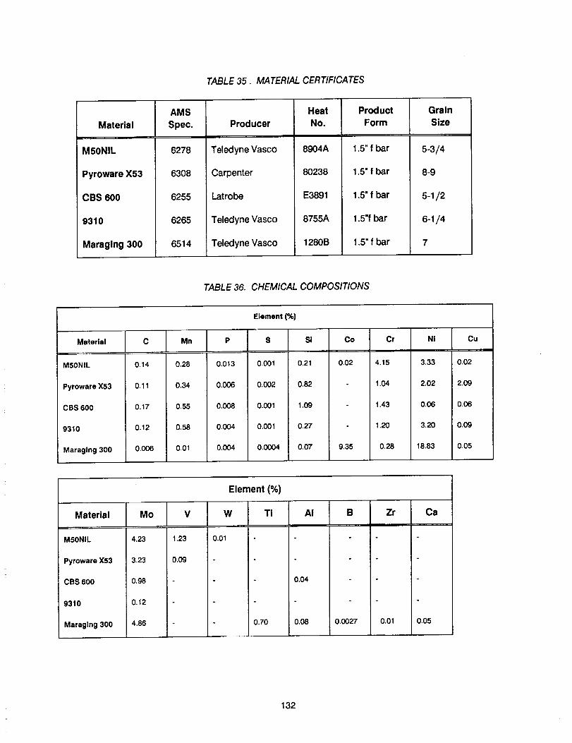
TABLE 35. MATERIAL CERTIFICATES
Material
M50NIL
Pyroware X53
CBS 600
9310
Maraging 300
AMS
Spec.
6278
63O8
6255
6265
6514
Prod ucer
Teledyne Vasco
Carpenter
Latrobe
Teledyne Vasco
Teledyne Vasco
HeatNo.
8904A
80238
E3891
8755A
1280B
ProductForm
1.5" f bar
1.5" f bar
1.5" f bar
1.5"fbar
1.5" f bar
GrainSize
5-3/4
8-9
5-1/2
6-1/4
7
TABLE 36. CHEMICAL COMPOSITIONS
Material
M50NIL
Pyroware X53
CBS 600
9310
Maraglng 300
C
0.14
0.11
0.17
0.12
0.006
Mn
0.28
0.34
0.55
0.58
0.01
0.013
0.006
0.008
0.004
0.004
Element (%)
S Si
0.001 0.21
0.002 0.82
0.001 1.09
0.001 0.27
0.0004 0,07
Co
0.02
9.35
Cr
4.15
1.04
1.43
1.20
0.28
NI
3.33
2.02
0.06
3.20
18.83
Cu
0.02
2.0g
0.06
0.09
0.05
Element (%)
Material Mo V A! Zr Ca
M50NIL
Pyroware X53
CBS 600
9310
Maraglng 300
4.23
3.23
0.98
0,12
4.86
1.23
0.09
0.01
W Ti
0.70
0.04
0.08 0.0027 0.01 0,05
132
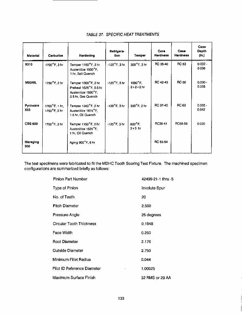
TABLE 37. SPECIFIC HEAT TREATMENTS
Material
9310
M5ONIL
PyrowareX53
CBS 600
Maraglng300
Carburlze
1700°F, 3 hr
1750°F, 2 hr
1700°F, 1 hr,
1750°F, 2 hr
1700°F, 3 hr
Hardening
Temper 1150°F, 2 hr
Austenitize 1500°F,
1 hr, Salt Quench
Temper 1300°F, 2 hr
Preheat 1625°F, 0.5 hr
Austenitize 1990°F,0.5 hr, Gas Quench
Temper 1350°F, 2 hr
Austenitize 1675°F,
1.5 hr, Oil Quench
Temper 1150°F, 2hr
Austenitize 1625°F,
1 hr, Oil Quench
/_oing 900°F, 6 hr
Refrigera-tion
-125°F, 3 hr
-120°F, 3 hr
-120°F, 3 hr
-120°F, 3 hr
Temper
300°F, 3 hr
IO00°F,
2+2+2hr
350°F, 2 hr
600°F,
3+3 hr
Core
Hardness
RC 35-40
RC 42-43
RC 37-40
RC39-41
RC 53-54
RC 63
RC60
RC 63
RC58-59
Case
Depth
(in.)
0.032-0.036
0,030"
0.035
0.035-
0.042
0.030
The test specimens were fabricated to fit the MDHC Tooth Scoring Test Fixture. The machined specimenconfigurations are summarized briefly as follows:
Pinion Part Number
Type of Pinion
No. of Teeth
Pitch Diameter
Pressure Angle
Circular Tooth Thickness
Face Width
Root Diameter
Outside Diameter
Minimum Fillet Radius
Pilot ID Reference Diameter
Maximum Surface Finish
42499-21-1 thru-5
Involute Spur
2O
2.500
25 degrees
0.1948
0.250
2.176
2,750
0.044
1.00025
32 RMS or 29 AA
133

Gear Part Number 42499-22-1 thru -5
Type of Gear Involute Spur
No. of Teeth 30
Pitch Diameter 3.750
Pressure Angle 25 degrees
Circular Tooth Thickness 0.1933
Face Width 0.500
Root Diameter 3.426
Outside Diameter 4.000
Minimum Fillet Radius 0.037
Pilot ID Reference Diameter 1.00025
Maximum Surface Finish 32 RMS or 29 AA
VI.B.I.iii Test Rig Description
The tests were performed on a hydraulically-powered, closed-loop, self-contained tooth pitting-scoring testfixture designed to test a single set of spur gears operating at a center distance of 3.125 inches at a maxlmumpinlon speed of 15,000 RPM. An isometric view of the NASA-Lewis Gear Fatigue Test Fixture, which alsoillustrates prlnclpal components of the MDHC scoring fixture's test gearboxes, is shown In Figure 58. Aphotograph of the MDHC scoring test fixture is shown in Figure 59. The maximum torque capacity of thescoring test fixture is 3100 in.-Ib, applied to the test pinion. The fixture contains separate lubrication systems forthe test gearbox and the slave gearbox, with each system containing a separate oil cooler. The lubrication
system for the test gears also incorporates an oil heater to provide a constant oil supply at the required oiltemperature. The fixture uses a three micron oil filter for the test gear lubrication system and incorporates chipdetectors. The test fixture provides lubrication and cooling oil to the test gears through one oil jet. Providing oll
into mesh, this Jet has one 0.045-inch diameter hole directing the oil flow. The stand has two inspection portswith removable transparent covers for viewing the condition of the test gear teeth.
134

Oil-seal
\
SIM-sysleqlo"" ell Inld
Figure 58. NASA-Lewis Gear Fatigue Test Fixture
Figure 59. MDHC Tooth Scoring Test Fixture
135 ORIGINAL PAGE
BLACK AND WHITE PHOTOGIRAPI_

Rotac Calibration Data ,.,To,qup• TorqueDown
Torque o - MeanTorque
4000 j .....................................................................i1#_ "f
I_Torque
In-lb
,ooo0 -,f---r----I----I I '....... I---' .... I ..... ' .... I.... ' - I- i I , "
0 100 200 300 400 500 600 700 800
METER PRESSUREIP91 )
Figure 60. Scoring Test Fixture Calibration Curve
The test fixture is instrumented with a display panel containing digital readouts and fault isolation lights withprovisions for recording equipment• It has a chip detector circuit which illuminates an indicator light andautomatically shuts off the fixture if the test specimens generate magnetic debris. The fixture has controlfeatures including automatic shutdowns for overspeed, high oil and bearing temperatures, and low oil pressureor excesslve pressure differential across the oil filter. The stand also Is capable of reading test time in tenths ofan hour.
The test fixture contains a Rotac hydraulic vane torque applier that was calibrated for fixture torque as hydraulic
pressure was applied in 75 psi (gage) increments from 0 to 750 psi and then decreased back to 0. A straightline fit of the torque vs. pressure data was found to be the accurate approximation of the values recorded asshown in Figure 60.
VI.B.l,iv T_st ProcQdure
During testing, each test gear set was mounted in the gear scoring fixture so that the pinion was fully engagedwith the exception of about 0.02 inch of its face width. This was done to avoid tooth overlap on the face of thegear member during subsequent tests with another pinion run on that same face. During tests, the test gearload and direction were such that the 20-tooth pinion was always the driving member, the bulk oil temperaturewas stabilized at 165°F, and the test gear oil pressure was set to 24•0 psi.
The gear sets were subjected to a break-In procedure prior to testing• The test gears were run 12 minutes at
reduced RPM and torque with the test gearbox oil temperature and pressure set to the operating conditions•
136

After break-in, the pinion gear tooth load was started at 600 in.-Ib torque at 10,000 RPM for the first load step.
Each gear specimen was operated in a series of load steps starting at 600 in.-Ib for 5-minute intervals. The
pinion torque was increased by 100 in.-Ib for each interval until scoring was observed after shut down. The tests
were shut down after each 5-minute Interval so the test gears could be visually inspected for scoring. The
inspections were made through the inspection port following easy removal of the inspection cover located on
the right side of the test gearbox housing.
Data recorded for each test included the test specimen material, part number, serial number, test date, start and
end time for each run, RPM for break-in and tests, torque for break-In and tests with pressure conversion, oil
temperature Into the gearbox, test gearbox oil pressurel slave gearbox oil pressure, inspection record and test
comments and operator's name and initials.
VI.B.l.v Result_
A summary of the test data is provided in Table 38. The test torque data, along with test speed, oil reservoir
temperatures and gear geometric parameters, were used to calculate flash temperatures [4]. Standard
summary statistics were then run against the flash temperatures. This data Is charted in Figures 61 and 62. The
most important determinant is the temperature at which a high percentage of the samples resist scoring. This is
indicated by the "mean - Standard Deviation (S.D.)" and "mean - 2 S.D." values In the figure. Mean minus S.D. is
the temperature in these tests at which there was a 15.87 percent chance of scoring (medium scorlng risk).
Mean minus 2 S.D. is the test temperature at which there was a 2.28 percent chance of scoring (low scoring
risk). In the AGMA tests, the medium scoring risk area was bounded on the upper side by a 30 percent chance
of scoring and on the lower side by a 5.5 percent chance of scoring. Using the minus 1 and minus 2 S.D. as a
bound for this area, in the MDHC tests, is a more conservative approach. Based on this criteria, the M50Nil
material and the CBS 600 have the highest scoring resistance, followed by X53, M300 and lastly AISI 9310.
Table 39 provides a summary of scoring flash temperatures of medium (-1 S.D.) and low (-2 S.D.) risk.
TABLE 38. SUMMARY OF SCORING TEST DATA
Torque Level, in.-Ib (25% Surface Scoring Observed)
Test 600 700 800 900 1000 1100 1200 1300 1400
M50NIL 6 27 21 12 3
X53 14 18 13 18 5 4
CBS 600 - 1 1 2 1 1
9310 1 4 26 41 23 1
300M 1 4 1 -
1500
1
No. of
Tests
70
72
6
96
6
* 250
* 252 tests were actually completed. Two test points run during early tests at 200°F oil reservoir
temperature (oil temp In) were invalidated due to tooth contact occurring on both the drive and
coast sides of gear teeth.
137

400
390
T 380
e370
m
P 360@
r 3508t 340
U 330r
e 320
°F310
3OO
M50Nil CBS600
I Ii
D Mean t[] Mean- S.D. J
|
[] Mean- 2 S.D. I
X53 M300 AISI9310
450
LLo 400
i
!
!l
Figure 61. Scoring Test Flash Temperatures
35_
--q---T---l_* CBS600
- o X53 -/_ M50NIL
- r] M300 -x AISt9310
300
0.1 02 05 tO 20
ART SC or_,
--4*--
J
--_
J
..... j JI _'J f+,I"_-
I_ .....
Test Oota
-1 .... !--] l,_z./4.,/ 7"_
X _ .....
"2_A...... []
S.0
Ii
j_
_1_ __V
XJ
J
I i L t_o.o io.o 3o.o 4o.o 5o.o eo.o ?o.o io.o . io.o t+.o _.o t*.o _,s N.i .++
Icod_l Pr o_+<Vt_illy- F_enlo_
Figure 62. Flash Temperature vs. Probability of Scoring
138

TABLE 39. FLASH TEMPERATURES (OF), SCORING RISK
Materials
M50NIL
CBS 600
X53
M300
AISI 9310
Medium Risk
Mean - 1 S.D.
372
371
355
338
332
Low Risk
Mean - 2 S.D.
356
351
334
328
318
VI.B.l.vi Discussion of Results
The significance of the results is that based on a scoring mode of failure, uslng the best gear steel (M50NIL) in
this test would provide an Increase of 389 ln.-Ib of operating torque with the same probability of scoring as the
AISI 9310 steel (at -2 S.D.). AISI 9310 steel was rated at 700 in.-Ib with a -2 S.D. probability of scoring, so this
represents a 56% improvement in load carrying capability. Also at -2 S.D. probability, CBS 600 provides an
increase of 221 in.-Ib torque (32% Improvement), X53 an Increase of 112 in.-Ib torque (16% improvement) and
300M an increase of 33 in-lb torque (5% Improvement). As can be seen in Table 40, only six samples of the CBS
600 and M300 test materials were used. This gives their results a lower confidence level than the other
materials.
TABLE 40. TEST SPECIMEN MATERIALS AND QUANTITIES
Material
M50 NIL
X53 Pyro.
CBS 6O0
AISI 9310
300M
Spec.
6278
6308
6255
6265
6514
Heat Treatment
Carburized and Hardened
Carburized and Hardened
Carburized and Hardened
Carburized and Hardened
Through Hardened
No. of
Tests
20
14"
12
17"*
12
*Will be 20 tests of X53 when completed (reference page 122)
**Will be 24 tests of AISI 9310 when completed (reference page 122)
Modern gear steels exhibit increased resistance to scoring that can be used to advantage. These benefits
should expand the envelope of gear design. Based on a scoring mode of tooth failure, results from the MDHC
scoring tests indicate a 56% improvement in load-carrying capacity with use of M50NIL steel, 32% improvement
with use of CBS600 steel, 16% improvement with use of X53 Pyroware and 5% improvement with use of 300M
steel. Results of other types of gear tests can be used in conjunction with this and previous scoring test results
to provide a recommended gear material for future aircraft application.
139

VI.B.2 S_inqleTooth Bending Fatigue Tests
VI.B.2.i Introduction
Gear tooth bending strength is one of the most important gear design parameters in drive system engineering.This report describes the test procedure and test results of single tooth bending fatigue tests performed on
advanced gear materials manufactured from near-net forglngs. The objective of the tests was to compare therelative bending strength of five advanced near-net forged gear steels. In addition, comparisons were madewith single tooth bending test results existing for standard forged gears of these materials. Tests were run atLWI, on 88 specimens consisting of X53 Pyroware, CBS 600, MSONIL, AISI 9310 and M300 gear materials. Thetest dg was designed to allow accurate placement of load at the highest point of single tooth contact on the testgear teeth. Test conditions were accurately determined using a calibrated load cell, load frequency and cycle
count measurement, strain gaged test gear teeth, and carefully recorded test data. AGMA bending stress wascalculated from raw test data, and best fit S-N curves for mean data and mean minus three sigma standard of
deviation were plotted for each material.
VI.B.2.il TeSt Article Description
Five near-net forged gear materials consisting of X53 Pyroware, CBS 600, M50NIL, AISI 9310 and M300 wereselected for tests of single tooth bending fatigue strength. The AISI 9310 and M300 steels were intended asbaseline gear materials for use In comparison with the high-hot-hardness X53, CB$ 600 and M50NIL steels. Thenear-net forging process was selected because it has the potential to increase gear fatigue life and improve theendurance limit. The process also makes more efficient use of raw materials and can greatly reduce or eveneliminate the need for secondary machining, depending on the quality class of gear required. The gearmaterials and test quantities used in the single tooth bending tests are identified as follows.
Part AMS Heat Make No. of
Nqmber Material _ Treatment From Tests
42499-21-11 M50 NIL 6278 Carburized and Hardened 42499-21-6 Forging 20
42499-21-12 X53 Pyro. 6308 Carburized and Hardened 42499-21-7 Forging 20
42499-21-13 CBS 600 6255 Carburlzed and Hardened 42499-21-8 Forging 12
42499-21-14 AISI 9310 6265 Carburized and Hardened 42499-21-9 Forging 24
42499-21-15 300M 6514 Through Hardened 42499-21-10 Forging 12
The five near-net forged materials were produced by the Eaton Corporation in Willoughby Hills, Ohio. Thematerial certificates and chemical compositions are outlined in Tables 41 and 42.
Each group of test specimens manufactured from the same material were from one heat and one melt of the
material and were heat treated in the same lot to minimize variation of the test population. One gear of eachmaterial was evaluated after carburizlng for microstructure and case depth at the profile and root. All the heattreatment operations were conducted at LWl Table 43 outlines the specific heat treatments applied to eachmaterial, and the actual case depth and hardness measured from the test gears. In addition, one gear of eachmaterial was evaluated for case depths at the same two locations after finish grinding.
140
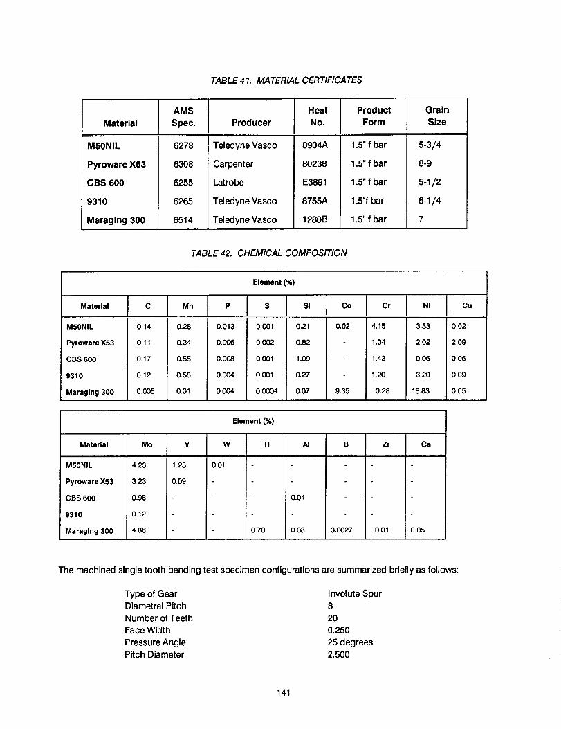
TABLE 41. MATERIAL CERTIFICATES
Material
M5ONIL
Pyroware X53
CBS 600
9310
Maraging 300
AMS
Spec.
6278
6308
6255
6265
6514
Producer
Teledyne Vasco
Carpenter
Latrobe
Teledyne Vasco
Teledyne Vasco
Heat
No.
8904A
80238
E3891
8755A
1280B
Product
Form
1.5" f bar
1.5" f bar
1.5" f bar
1.5"f bar
1.5" f bar
Grain
Size
5-3/4
8-9
5-1/2
6-1/4
7
TABLE 42. CHEMICAL COMPOSITION
Element (%)
Material C Mn P S Si Co Cr Ni Cu
M50NIL
Pyroware X53
CBS 600
9310
Maragin 9 300
0_14
0.11
0.17
0.12
0.006
0.28
0.34
0.55
0.58
0,01
0.013
0.008
0.008
0.004
0.004
0.001
0.002
0.001
0.001
0.0004
0.21
0.82
1.09
0.27
0.07
0.02
9.35
4.15
1.04
1.43
1.20
0.28
3.33
2.02
0.06
3.20
18.83
0.02
2.09
0.06
0.09
0.05
Element (%)
Material
M50NIL
Pyroware X53
CBS 600
9310
Maraglng 300
Mo
4.23
3.23
0.98
0.12
4.86
V
1,23
0.09
0.70
TI Ai
0.04
0.08
B
0.0027
Zr
0.01
Ca
0.05
The machined single tooth bending test specimen configurations are summarized briefly as follows:
Type of Gear Involute Spur
Diametral Pitch 8
Number of Teeth 20
Face Width 0.250
Pressure Angle 25 degrees
Pitch Diameter 2.500
141

Base Diameter 2.266Outside Diameter 2.750Root Diameter 2.176Minimum Fillet Radius 0.054Circular Tooth Thickness 0.1933
Eight of the 20 gear teeth were removed to eliminate possible Interference with the test fixture. As shown in theFigure 63 view taken from Lucas Western drawing 42499-21, there were four test teeth on each test gear.Before starting the tests, the circular tooth thickness, fillet radius, root diameter, outside diameter, and rootsurface finish of each gear were measured and recorded. These values were used to accurately calculate the
AGMA bending stress [55] for each gear.
TABLE43. HEAT TREATMENTS, CORE/CASE HARDNESS AND CASE DEPTH AT PITCH LINE
Material
9310
M50NIL
PyrowareX53
CBS 600
Maraglng300
Carburlze
1700°F, 3 hr
1750°F, 2 hr
1700°F, 1 hr,
1750°F, 2 hr
1700°F, 3 hr
Hardening
Temper 1150°F, 2 hr
Austenitize 1500 °F,
1 hr, Salt Quench
Temper 1300°F, 2 hr
Preheat 1625°F, 0.5 hr
Austenitize 1990°F,
0.5 hr, Gas Quench
Temper 1350°F, 2 hr
Austenitize 1675°F,
1.5 hr, Oil Quench
Temper 1150°F, 2 hr
Austenitize 1625°F,
1 hr, Oil Quench
Aging 900°F, 6 hr
Refrlgera-tJon
-125°F, 3 hr
-120°F, 3 hr
-120°F, 3 hr
-120°F, 3 hr
Temper
300°F, 3 hr
1000°F,
2+2+2 hr
350°F, 2 hr
600°F,
3+3 hr
CoreHardness
RC 35-40
RC 42-43
RC 37-40
RC39-41
RC 53-54
Case
Hardness
RC63
RC6O
RC63
RC58-59
Case
Depth
(in.)
0.032 -0.036
0*030-
0.035
0.035 -0.042
0.030
Vl.B.2.iii Test Rig Description
The test rig for single tooth bending tests included a single tooth bending test fixture (shown in Figures 64 and65), designed by LWI, and an MTS Model 800 materials test system. The test fixture was mounted on the baseplate of the MTS load frame. The MTS Model 810 machine Is a servohydraulic, closed-loop control systemdesigned for test of fracture mechanics, fatigue and basic material properties. The slngle tooth bending testfixture was designed so that the test tooth was loaded at the highest point of single tooth contact, based on a1:1 gear ratio, while the reaction tooth was loaded at the lowest point of single tooth contact. The fixture designallows tests of 1.5 to 6.0-inch pitch diameter spur gears with face widths up to 0.5 inch. Both the load andreaction anvils can be repositioned to accommodate various tooth heights along the line of action for involute
spur gears. The fixture also has strip chart recorder and signal generator compatibility. A drip lubricationsystem Is incorporated to prevent spalling of the test speclmens. Other features include a crack detector circuit
enabling automatic shutdown of the fixture, an oil filter and a digital readout. The fixture also has a customfurnace which can be used for elevated temperature tests at up to 800°F.
142

• I ,. ,-':
I • SO0
R 1.120
5X
16v//ENTlRE
EO. SPACED
TOOTH PROFILE
MOUNTING j
SURFACE
. 250
2.750vwm
VJh J
f_JfJA
REMOVE TEETHAS SHOWN.
Figure 63. Detail Views of Test Gears
Load applied to the test gear was measured with a calibrated commercial load cell which was mounted under
the loading stud, as shown in Figures 64 and 65. The load cell was calibrated per ASTM standards. The load
anvil was adjusted to the desired contact position by stroke control of the loading stud. The test gear was then
mounted on the fixture and the reaction anvil was slightly adjusted so that both load and reaction teeth were in
contact. A load of 100 Ib was then applied to the test tooth, and the positioning of anvils rechecked. The
minimum load was maintained at 100 Ib during all tests to ensure that constant contact was maintained and
impact loads were avoided. Thus the mean load was always 100 lb higher than the alternating load during test
runs.
The crack detector circuit was employed through instrumentation of all test teeth with crack wires to ensure that
each test could be stopped at a fixed crack length of approximately 0.070 inch at the root fillet area. The wire
was bonded to both sides of the test tooth at approximately 1/32-inch from the root radius, and then integrated
into the control circuit of the test machine. Failure was defined as a crack which progressed through the wire
until the crack wire broke. In addition to automatic test rig shutdown due to crack wire breakage, the system
would also be shut down due to detection of error in the load range value, detection of error in limit values for
both load and stroke, and manual emergency stop.
143

ORIGINAL PAGE
aLACK AND WHIYE PHOTO(:t,R/IIPH
Figure 64. Test Tooth and Load Anvil
Figure 65. Single Tooth Bending Fatigue Test Fixture
144

VI.B.2.iv Test Procedure
All single tooth bending fatigue tests were executed at the LWI, Applied Technology Division facility using thepreviously described test fixture mounted on an MTS servo-controlled, closed-loop, hydraulic test machine.Prior to testing, the test gear teeth were instrumented with strain gages as shown in Figure 66 so that actualgear tooth root stress could be measured and plotted against the applied normal load. The strain gages werelocated at the point on the tooth root of AGMA maximum bending stress [55]. Strain gages of 0.015-inch lengthwere selected based on the test gear root configuration. A cast was made of the tooth space and used as atemplate for laying and pressing the two strain gages at the desired locations.
Conlact Area
\\
!I
t
W- 1/32"
W
Strain Gage No. 2
S - 0.040" - 0.060"
Strain Gage No. 1
Strain Gages located at
the positionof AGMA
maximum bending stress.
Figure 66. Strain Gage and Crack Wire Placement
The loading frequency for all tests was 30 Hz. Any gear tooth which ran at a specific load level for 3x10⁶ cycleswas considered a run-out for this single tooth bending fatigue test program. The first tests of the M50NIL, X-53and CBS 600 material gears were run at approximately 2031 + 1931 Ib (280 ksi maximum). The first 9310 steel
gear test was run at approximately 2172 + 2072 Ib (300 ksi maximum), while that of maraging 300 steelmaximum was run at 1748+1648 Ib (240 ksi maximum). If the first test was a runout, load was increased to
yield a 40 ksi maximum bending stress Increase for the second test. If the first test yielded a tooth failure, load
145

was decreased to yield a 20 ksi drop in maximum bending stress. Subsequent tests were increased ordecreased in a similar manner, with the goal of attaining a few run-outs and having most of the remaining failurepoints clustering about the bend or "knee" of the S-N curve attained for each material. In addition, the loadlevels at which failures occurred were usually run for more than one test to give some idea of the test resultvariance seen at the same loads.
Data recorded for each test run Included test gear serial number, test gear material conditions, test gearconfiguration data, test tooth number, applied normal loads (maximum and minimum), calibrations of straingaged tooth, cycles to failure, failure mode, frequency of applied load, and test temperature.
The equivalent bending stresses for the test load values were calculated, based on the AGMA tooth bending
stress formula [55], as follows:
St =Wt Ko Pd Ks Km
KvFJ
Where
St = Calculated tensile bending stress at the root of the tooth, pslWt = Transmitted tangential load at operating pitch diameter, IbKo = Ovedoad factor
Kv = Dynamic factorPd = Diametral pitch
F = Facewidth, inchKs = Size factor
Km = Load distribution factor
J = Geometry factor
For this testing program,
Ko = Kv = Ks = Km = 1.0 and Wt = Wn cos (_)
Where,
Wn = Applied normal load= Pressure angle at the pitch diameter
Therefore,
Wn • Cos (_t •PdSt-F*J
In this single tooth bending test program, the load was applied at the worst load position, I.e., at the highestpoint of single tooth contact. The "J" factor was calculated by the Lucas Western SHAG program which wasdeveloped according to AGMA Standard (55). So, for a 3000 Ib applied normal load, the maximum bendingstress was calculated as:
3000 • Cos (25°) • 8St-0.25 • 0.4104035
= 212 ksl
146

VI.B.2.v Results
The basic raw data is shown in Tables 44, 45, 46, 47, and 48. All the fatigue lives were rounded to the nearest
100 cycles. The real significance of this data can only be gaged when it is subjected to a statistical evaluation.
Five bending strength formulae were investigated and applied to the fatigue test spur gear configurations -
Lewis, Dolan-Broghamer, Heywood, Kelly-Pederson, and AGMA. The AGMA method gave the smallest
deviation from the measured stress for spur gears (56). Therefore, S-N curves were fitted to the tooth fatigue
data with respect to AGMA calculated stress in this gear tooth bending fatigue test program. The general
approach involved analyzing the data statistically in order to define the sample mean, the standard deviation,
and the mean endurance limit. This data then can be used to compare various materials and to make
reasonable projections of the allowable bending stress for a given material under realistic design conditions.
Runouts from the fatigue test data were not included when determlnlng a best fit curve. Runouts were shown in
the S-N curve for information only and were clearly distinguished from the finite life data points by the use of
arrows. The number of arrows indicates the number of tests that were run at that specific stress level. Because
the S-N relationship was reasonably approximated by a curve for a specific interval of stress, it was not
recommended that the S-N curve be extrapolated outside the interval of testing (57).
TABLE 44. MSONIL SINGLE TOOTH BENDING FATIGUE TEST DATA
Material: Carburized M50NIL Steel per AMS 6278
Test Temperature: RT Case Depth (Inch): 0.030-0.035
(at pitch line)
Case Hardness: RC 60
Core Hardness: RC 42-43
Test No.
1
2
3
4
5
6
7
8
9
10
11
12
13
14
15
16
17
18
19
2O
AGMA Max. Bending Stress, ksi
280
260
320
280
320
340
300
340
300
300
280
290
29O
290
290
290
28O
320
340
280
Cycles to Failure
369,300
Run Out
41,100
Run Out
10,000
19,500
32,OOO
4,900
18,100
24,800
Run Out
22,600
157,000
22,900
52,200
38,200
Run Out
31,100
5,000
91,500
147

TABLE 45. X53 SINGLE TOOTH BENDING FATIGUE TEST DATA
Material: Carburized X53 Steel per AMS 6278
Test Temperature: RT Case Depth (Inch): 0.035-0.042
(at pitch line)
Case Hardness: RC 63
Core Hardness: RC 37-40
Test No.
1
2
3
4
5
6
7
8
9
10
11
12
13
14
15
16
17
18
19
20
AGMA Max. Bending Stress, ksi
28O
320
340
300
320
340
3OO
3OO
290
3O0
3OO
320
34O
30O
320
340
295
360
360
36O
Cycles to Failure
Run Out
52,600
8,200
1,791,600
16,700
10,500
55,000
26,400
Run Out
781,600
Run Out
88,400
9,300
553,400
33,200
23,600
75,1 O0
15,900
7,100
7,600
148

TABLE 46. CBS 600 SINGLE TOOTH BENDING FATIGUE TEST DATA
Material: Carburized CBS 600 Steel per AMS 6255
Test Temperature: RT Case Depth (Inch): 0.030
(at pitch line)
Case Hardness: RC 58-59
Core Hardness: RC 39-41
Test No.
1
2
3
4
5
6
7
8
9
10
11
12
AGMA Max. Bending Stress, ksi
28O
320
300
290
320
300
290
290
280
290
340
340
Cycles to Failure
Run Out
19,700
15,200
Run Out
23,800
74,400
33,900
34,200
Run Out
Run Out
12,200
17,500
Figures 67, 68, 69, 70, and 71 show the mean S-N curve (50 percent failure) and the curve of the mean minus 3
sigma for each material. The mean endurance limits, standard deviations, and the mean endurance limit minus
3 sigma are shown in Table 49 and Figures 67 through 71. For comparing the bending fatigue strength, all the
mean S-N curves of the five materials are plotted in Figure 72.
The failure modes have been evaluated and all were the typical failures of the tooth root fillet bending fatigue.
Cracks were found in the root areas of either one side or both sides of test teeth with a length of approximately0.070 inch.
VI.B.2.vi Discussion of Results
Based on the specific heat treatments of each material (as previously shown in Table 43), Pyroware X53 has the
greatest tooth bending fatigue strength. AISI 9310 is the material of the least bending fatigue endurance. The
five materials are rated in terms of tooth bending fatigue strength as follows:
1. X53
2. CBS 6OO
3. M5ONIL
4. Maraging 300
5. 9310
149
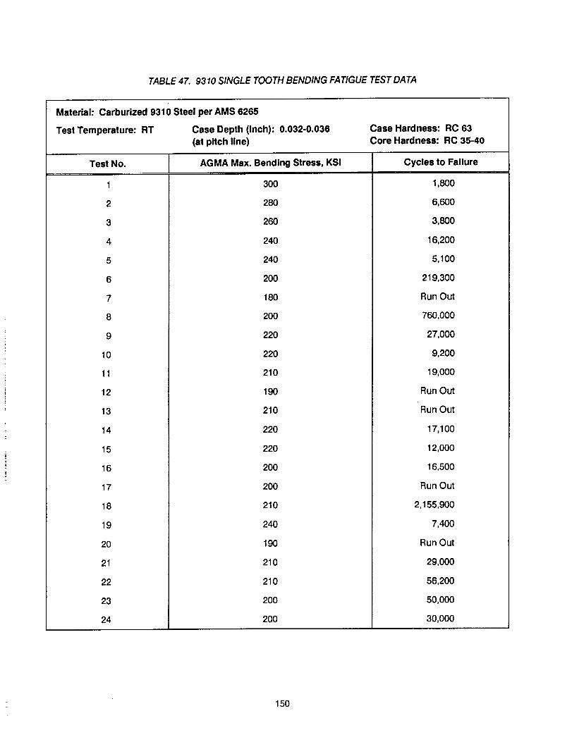
TABLE 47. 9310 SINGLE TOOTH BENDING FATIGUE TEST DATA
Material: Carburized 9310 Steel per AMS 6265
Test Temperature: RT Case Depth (Inch): 0.032-0.036
(at pitch line)
Case Hardness: RC 63
Core Hardness: RC 35-40
Test No.
1
2
3
4
5
6
7
8
9
10
11
12
13
14
15
16
17
18
19
20
21
22
23
24
AGMA Max. Bending Stress, KSI
3OO
280
260
240
240
200
180
2O0
220
220
210
190
210
220
220
200
20O
210
240
190
210
210
2OO
20O
Cycles to Failure
1,800
6,600
3,800
16,200
5,100
219,300
Run Out
760,000
27,000
9,200
19,000
Run Out
Run Out
17,100
12,000
16,500
Run Out
2,155,900
7,400
Run Out
29,000
56,200
50,000
30,000
150

TABLE 48. M300 SINGLE TOOTH BENDING FATIGUE TEST DATA
Material: Through-hardened Maraging 300 Steel per AMS 6514
Test Temperature: RT Case Depth (Inch):
(at pitch line)
Case Hardness: RC
Core Hardness: RC 53-54
Test No.
1
2
3
4
5
6
7
8
9
10
11
12
AGMA Max. Bending Stress, KSI
240
220
260
220
200
240
260
210
2OO
280
280
210
Cycles to Failure
121,400
687,700
35,900
120,800
Run Out
42,500
89,1 O0
141,300
Run Out
30,000
39,900
93,1 O0
Comparing the single tooth test results of these five near-net forged materials with that of Lucas Western's
conventional test gears made from bar stock, it is concluded that:
The tooth bending fatigue strengths of near-net forged X53, CBS 600, M5ONIL, and Maraging 300 are only
slightly better than that of conventional gears.
The tooth bending fatigue strength of conventional 9310 gears is greater than the near-net forged 9310
gears.
151

AGMA
MAX
BENDING
STRESS
kSI
SINGLE TOOTH BENDING FATIGUE TEST AT RT_URIZED MSONIL STEEL PER AMS G278
368
34e •
328 •0
3oo oo
288 g
268
240
2"28
288
188
168
148
T_oth Profile i Boot SUrtK* rlJLohs $| elS
_IU/_LLt_ __ Vacmm cmrlmriled *.750 F 6 2 hr
Tempecod 1350 F, _ hr • _rel_lited 1625 F,
171 Islr _ Aueten|t_sod 19110 P, 112 hr, Gq 4
h(r_letitod -120 F, $ _r • TllllpqJtOd 1000er,
|*l_2hr.
Caoo Doptht 0.O$0-0.O3S tn.
Itmrdnemo, Cue ,,. E _ C,oI_ ,,. I¢ 42-4'm
Ibm I_durmce LlJdtl _tlJl tel
Stsndard hvletfou (I)i 11.1 ttLIben I_lurl_Ce - _ , 141 tel
_m It)0 No_ Curve (l)t Jleu - 3e
' I ' I
10 lee
e_..( 1 )
(2)
I_Y-20- l gg2I
I,it_ le, OOe
T_ OF' CYCLES TO FA[LUIRE
BENDING
STRESS
KS1
Figure 67. Best Fit S-N Curve of Single Tooth Bending Fatigue TestsMaterial: M5ONIL
SINGLETOOTHBENDINGFATIGUETESTAT RTCARBJRIZEDXS3 STEELPER _ G308
36e
368
340 • •
328 • •
31_ (ll
288
268
24B
220
260
188
14O
(2l
hot'- IPtofllo Ib _ I_grtlce IPbiloits $| INS
IhUt_, VKim csflmrJsed 17MI F. 1 hiE'
;1130 It, I It¢ '_ ?_mtd 1)5i Ye J kr #Auettqsltlsed 1113 F,I.S Its, 0q t hftlloritod
-Ill'F, I Itf * Teegetd SSI*IPo t br
_soe DelPtk* 0.Q|5-0.|41 In.
limfdlmonmee ¢80e -- 8C 65 Cot_ w lie Sl.41i
Nora IbulkJfance LtmJ¢o |11 I_1
stslded I)ev|St|_ leP0 lS.i JteJ
Cram Ill0 Hoam _ (|It Ihlln . Sm
' | ' I
l0 IBO
HAY-20- 1992
I
1.888 IO, NO
TIDRAM)SOFCYCLES TOFAILURE
Figure 68. Best Fit S-N Curve of Single Tooth Bending Fatigue Tests
Material: X53
152

AGHA
MAX
BEND!NG'
STRESSe
KSI
AGMA
MAX
8ENDING
STRESS#"
KSI
3_
368
348
328
308
288
268
248
2_
208
188
IG8
148
SINGLE TOOTH BENDING FATIGUE TEST AT RTCARBURIZED CBS Gee STEEL PER AMS 62(35
'e.,.,. ( ! )
(2)
Tooth Prof|le & loot 8urfl¢e Plnteh, 3|
]hI_.__31i_, vicuul cirht'|sed 1700-F, $ hr
+ Tempered 1150 F, 4 hr 4. au|tou|t|led 1123eF,
I hr, Oq ÷ RlfrJlierlted 0120 F, 3 hr ÷
Tempered li_ IP, 3 • 3 hrClio Deptht 0.030 I,m.
UmrdnolmJ Csee - It(: 3li-3l COlrO - ItC $9-11
14emt I_duri_:o Ll_[te |13 bi
litandard Doviatloo (Ir)l 14.4 I(ei
Hoe,n U'ndursnce . $g i 15 5, Eli
Cir_ (l)J ISeu Cu¢_l (1). Nero - 3/
' I ' I
18 IOO
MAY-20-I gg2I
Io_ 18._
TI-EoANDS OF CYCLES TO FAILURE
Figure 69. Best Fit S-N Curve of Single Tooth Bending Fatigue TestsMaterial: CBS 600
SINGLE TOOTHBENDING FATIGUE TEST AT RTCtd:_BL)R[ZEDQ318 STEEL PER Pt'lS G265
380
Tempered 1130 F. | br 4 kiotemltlte| 1500 F,
I kr, lialt quo_ck * !liolrtliermted -120 F. $ hr34B ,I, Teipered 500 r, 3 bt'.
CIIO I_pthJ li.lJS|-I.0$l JlI.
328 IterdMeel C_oe - ItC Is Cofo., I¢ 55-40
HOSe Indurllce Ltmiti 1$| 10t
liUm4ir4 Dovlmtlml (#)l 15 letNon lindurince - 3G I 132 gilL
Curvo (1)0 Non Curve (lie Nooa -
240 • •
228
0-0-_ ( 1 )180 e-.-
IGO 12)
140 HAY-2O- 1992I I I' I I ! I
IO lee 1,880 le.eeo
OF CYCLES TO FAILURE
Figure 70. Best Fit S-N Curve of Single Tooth Bending Fatigue TestsMaterial: 9310
153
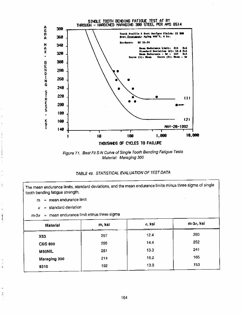
AGMA
MAX
BENDING
STRESS
KS!
3_
368
34e
320
3_e
280
268
248
229
2oe
189
168
149
SINGLE TOOTHBENDING FATIGUE TEST AT RTTHROUGH HARDENEDHARAGING3_ STEEL PER AHS G_l 4
J rui
_ '_tb ,_,,L. , ,_t k.,,.. ,ill|.ll. ,, .
\ \ t4em endurance Llnttt 21Q tet% |teudsrd Dev|atfoe (eje |f.| Kef
\ % Hen 8nduruee . _Je , 115 let
• •
• o4.,=.-11 )v
(2)
HAY 28 Igg2I v I I
le iw 1,888 19_
TFIOUS/#¢_ OF CYCLESTO FAILURE
Figure 71. Best Fit S-N Curve of Single Tooth Bending Fatigue TestsMaterial: Maraging 300
TABLE 49. STATISTICAL EVALUATION OF TEST DATA
The mean endurance limits, standard deviations, and the mean endurance limits minus three sigma of singletooth bending fatigue strength.
m = mean endurancelimit
<_ = standard deviation
m-3o = mean endurance limit minus three sigma
Material
X53
CBS 600
M5ONIL
Maraging 300
9310
m, ksl
297
295
281
214
192
CTºksi
12.4
14.4
13.3
16.2
13.0
m-3_, ksi
26O
252
241
165
153
154

ABRA
HAX
BEND!NG
STRES$
KS!
SINGLE TOOTHBEHI)ING FATIGUE TEST AT RTCOHPARISOHOF HEAN S/N CURVESFOR FIVE GEAR HATERI_eI.S
388
34O
328
388
288
26O
248
228
288
188
X53CBS 68_
HSI_iL
168
140 HAY-28-1992i I I
18 188 1,888 I0,_
OF CYCLES TO FAILW
Figure 72. Comparison of Best Fit S-N Curves for Five Gear Materials
The possible reasons for the fatigue strength differences between near-net forged gears and conventional gears
are outlined below:
1. Size Effe?t. The conventional test gears have a greater size (8 DP, 3.75-inch pitch diameter).
2, Case Depth. Some case depth of carburlzed conventional gears are only 0.020 inch, which is shallower
than the near-net forged gears.
. Due t0 the Difference in Gear Man_Jfecturinq Pr0ce_ses. Further research work may be necessary to
investigate the bending fatigue strength difference between the near-net forged gears and conventional
gears.
In order to obtain more data in the high cycle fatigue range and reduce the standard deviations, more single
tooth tests of material CBS 600 and Maraging 300 are required to achieve a better statistical evaluation of test
data. Also, to compare the tooth bending fatigue strength between near-net forged gears and conventional
gears, it is recommended that two groups of test gears with the identical gear size/configuration and the same
case depth should be used to conduct the single tooth bending fatigue tests.
Finally, the AGMA formula of tooth bending stress was selected to correlate the test data, since AGMA
calculated stress best matched experimentally measured stress. Since the LWI Shag Program is based on
AGMA equations [55], it also allows the data derived herein to be used for design and analysis directly. Since
the test gears used are actual full sized gears and not specimens, the data obtained from the testing does not
need to be adjusted to size.
155
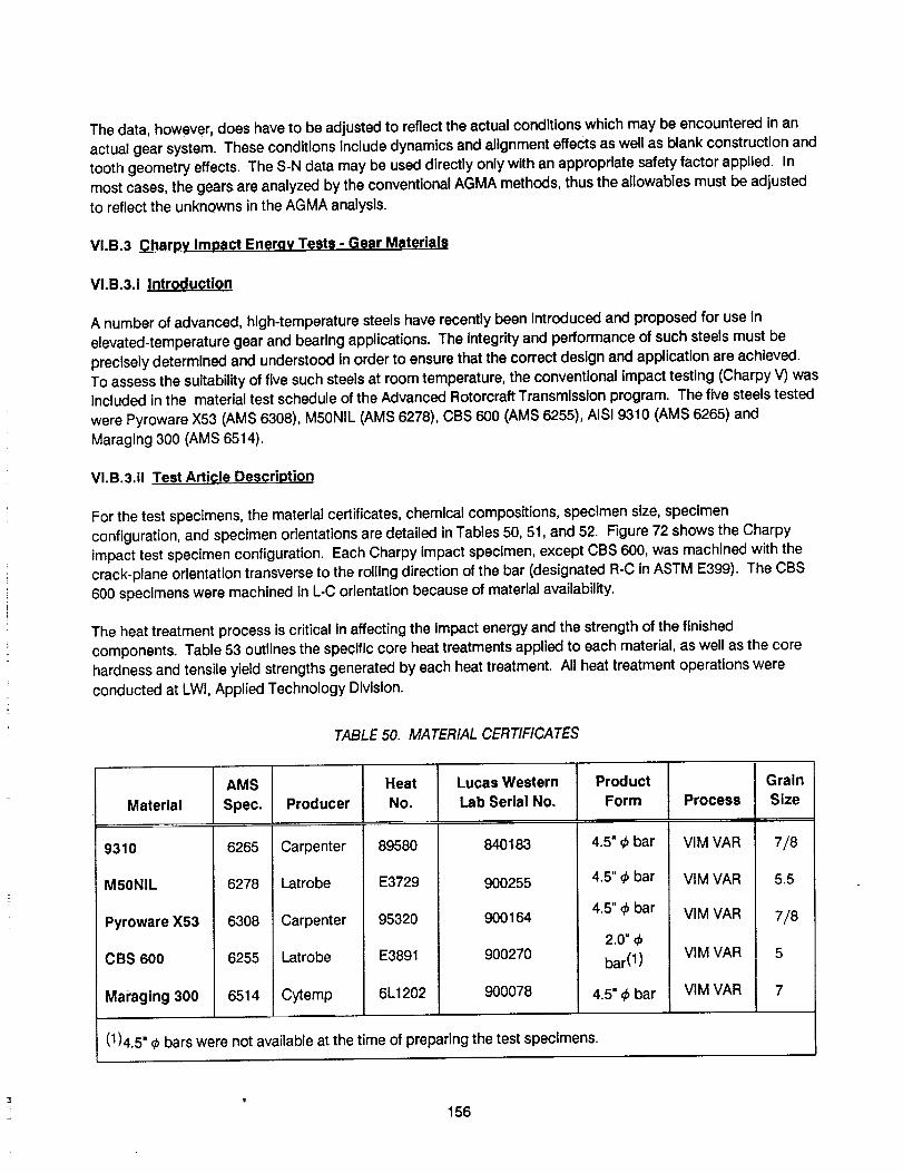
The data, however, does have to be adjusted to reflect the actual conditions which may be encountered in anactual gear system. These conditions include dynamics and alignment effects as well as blank construction andtooth geometry effects. The S-N data may be used directly only with an appropriate safety factor applied. Inmost cases, the gears are analyzed by the conventional AGMA methods, thus the allowables must be adjustedto reflect the unknowns in the AGMA analysis.
VI.B.3 .C_harpyImpact Energy Tests - Gear Materials
VI.B.3.i Introduction
A number of advanced, high-temperature steels have recently been Introduced and proposed for use Inelevated-temperature gear and bearing applications. The integrity and performance of such steels must beprecisely determined and understood in order to ensure that the correct design and application are achieved.To assess the suitability of five such steels at room temperature, the conventional impact testing (Charpy V) wasincluded in the material test schedule of the Advanced Rotorcraft Transmission program. The five steels testedwere Pyroware X53 (AM$ 6308), M50NIL (AMS 6278), CBS 600 (AMS 6255), AISI 9310 (AMS 6265) andMaraging 300 (AMS 6514).
VI,B.3.ii Test ArtiGle Description
For the test specimens, the material certificates, chemical compositions, specimen size, specimenconfiguration, and specimen orientations are detailed in Tables 50, 51, and 52. Figure 72 shows the Charpyimpact test specimen configuration. Each Charpy impact specimen, except CBS 600, was machined with thecrack-plane orlentatlon transverse to the rolling direction of the bar (designated R-C in ASTM E399). The CBS600 specimens were machined in L-C orientation because of material availability.
The heat treatment process is critical in affecting the Impact energy and the strength of the finishedcomponents. Table 53 outlines the specific core heat treatments applied to each material, as well as the corehardness and tensile yield strengths generated by each heat treatment. All heat treatment operations were
conducted at LWI, Applied Technology Division.
TABLE 50. MATERIAL CERTIFICATES
AMS
Material Spec. Producer
9310 6265 Carpenter
M50NIL 6278 Latrobe
Pyroware X53 6308 Carpenter
CBS 600 6255 Latrobe
Maraging 300 6514 Cytemp
HeatNo.
89580
E3729
95320
E3891
6L1202
Lucas WesternLab Serial No.
ProductForm
840183 4.5" 4 bar
900255 4.5" 4 bar
4.5" 4 bar900164
2.0"4
900270 bar(l)
900078 4.5"4 bar
GrainProcess Size
VIM VAR 7/8
VIM VAR 5.5
VIM VAR 7/8
VIM VAR 5
VIM VAR 7
I!( )4.5 4 bars were not available at the time of preparing the test specimens.
156

TABLE 51. CHEMICAL COMPOSITION
Material
9310
M50NIL
Pyroware)(53
CBS 600
Maraglng3O0
C
0.10
0.12
0.12
0.17
0.01
Element (%)
Me I P S i s,pcolcrI ., icol olv rw0.65 0.006 0.004 0.27 1.31 3.21 0.03 0.15 -
0.21 0.015 0.004 0.17 0.02 4.15 3.48 0.04 4.28 1.24 0.03
0.28 0.009 0.00016 0.66 0.96 1.97 1.90 3.21 0.10
AI
0.54 0.005 0.001 1.12 1 _46 0.02 0.06 0,93 0.05
0.01 0.001 0.004 0.05 9.17 0.28 18.52 0.05 4.91 0.68 0.12
Vl.B.3.iii Test Rig Description
The Charpy Impact Tester, made by Tinius Olsen, is a pendulum-type testing machine of rigid construction and
capacity more than sufficient to break the specimen In one blow. The machine used was verified on April 4,
1990, which was within one year prior to the January 1991 testing month. The test results using this machine
were within the allowed variation range of the National Institute of Standards and Technology (NIST).
TABLE 52. SPECIMEN SIZE, SPECIMEN CONFIGURATION, AND SPECIMEN ORIENTATION
AMS Specimen Specimen Speclmen
Material Specification Size Configuration (1) Orientation (2)
9310 6265 0.394" x 0.394", Full Charpy (Simple Beam) RC
V-Notch, Type A
M50NIL
Pyroware X53
CBS 600
Maraglng 300
6278
63O8
6255
6514
0.394" x 0.394", Full
0.394" x 0.394", Full
0.394"x 0.394", Full
0.394" x 0.394", Full
Charpy (Simple Beam)
V-Notch, Type A
Charpy (Simple Beam)
V-Notch, Type A
Charpy (Simple Beam)V-Notch, Type A
Charpy (Simple Beam)V-Notch, Type A
RC
RC
LC
RC
(1)
(2)See Figure 72.Use the crack plane orientation code in ASTM E399.
L = direction of maximum grain flow (the direction normal to the crack plane).R = radial direction (the direction normal to the crack plane).
C = circumferential or tangential direction (the expected direction of crack propagation).
157
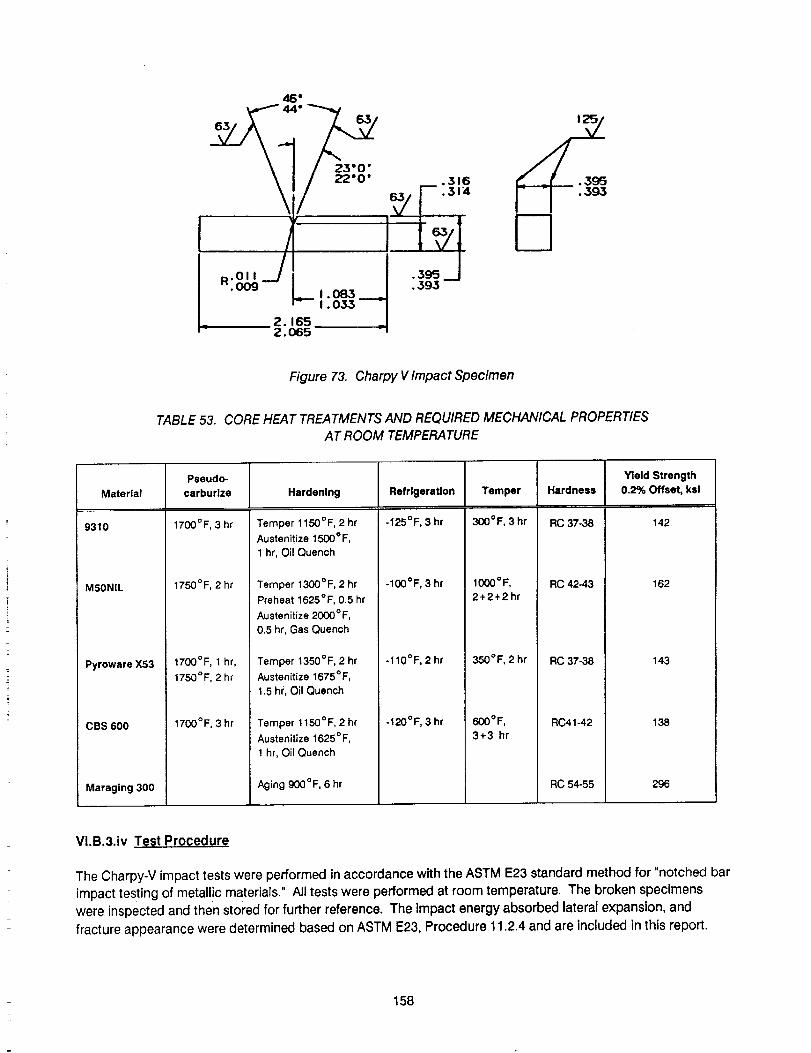
46 •
1/ / 23"o"/ I 22*0*/ I ¢._ v .316
. 2. 65 JZ. 065" 7
. 395.393
Figure 73. Charpy V Impact Specimen
TABLE 53. CORE HEAT TREATMENTS AND REQUIRED MECHANICAL PROPERTIESAT ROOM TEMPERATURE
Material
9310
M5ONIL
Pyroware X53
CBS 600
Maraging 300
Pseudo-
carburlze
1700°F, 3 hr
1750°F, 2 hr
1700°F, 1 hr,
1750°F, 2 hr
1700°F, 3 hr
Hardening
Temper 1150°F, 2 hr
Austenitize 1500°F,
1 hr, Oil Quench
Temper 1300°F, 2 hrPreheat 1625°F, 0.5 hr
Austenitize 2(X)OoF,
0.5 hr, Gas Quench
Temper 1350°F, 2 hr
Austenitize 1675°F,
1.5 hr, Oil Quench
Temper 1150°F, 2 hr
Austenitize 1625°F,
1 hr, Oil Quench
Aging 900°F, 6 hr
Refrigeration
-125°F, 3 hr
-IO0°F, 3 hr
-110°F, 2 hr
-120°F, 3 hr
Temper
300°F, 3 hr
IO00°F,2+2+2hr
350°F, 2 hr
600°F,
3+3 hr
Hardness
RC 37-38
RC 42-43
RC 37-38
RC41-42
RC 54-55
Yield Strength0.2% Offset, ksl
142
162
143
138
296
Vl.B.3.iv Test procedure
The Charpy-V impact tests were performed in accordance with the ASTM E23 standard method for "notched barimpact testing of metallic materials." All tests were performed at room temperature. The broken specimenswere inspected and then stored for further reference. The Impact energy absorbed lateral expansion, and
fracture appearance were determined based on ASTM E23, Procedure 11.2.4 and are included in this report.
158

2X I. 375-_,-
• 5oo -- _ .5oo1 1
Figure 74. Tension Test Specimen
In addition to the Charpy impact tests, five tensile tests of each material were performed at room temperature tocheck the validity of the heat treatment cycles. The tensile bars were heat treated in the same batch with theCharpy rectangular bars, prior to machine finishing. Figure 73 shows the tensile test specimen configuration.All tensile testing was carried out in accordance with ASTM E8.
VI.B.3.v Results
Following tests, the percent shear fracture was determined and recorded. Lateral expansion was measuredfrom the two halves of each broken specimen. The impact energy data was statistically analyzed and Table 54presents a summary of the impact energy mean values, standard deviations and predicted ranges of meanvalue at 99 percent confidence level. Also included in the table are the average tensile test properties for tensiletest specimens of the five materials.
Based on the core heat treatments conducted for each material and summarized in Table 4, AISI 9310 is the
toughest material and M50NIL is the least tough. Pyroware X53 was found to be the second toughest, with CBS600 third, and maraging 300 fourth. These results used in conjunction with results of other tests contained inthis report, as well as results of previously performed tests, provide the design engineer with good indication ofthe material to choose for the requirements of his application.
159
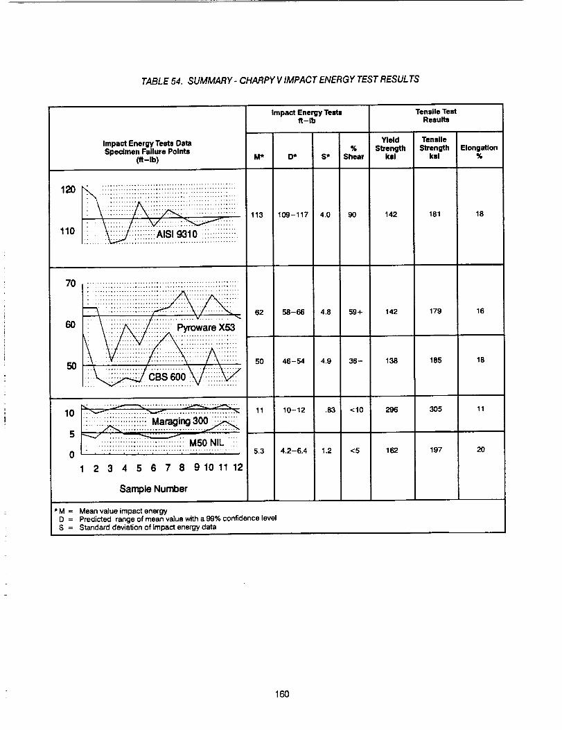
TABLE 54. SUMMARY- CHARPY V IMPACT ENERGY TEST RESULTS
impact Energy Testsft-lb
Impact Energy Tests DataSpecimen Failure Points %
(ft-lb) M* D* S* Shear
110 _ _:_i:.::AISI9310 iiiiii!i!iiii.
70
6O
*M=D=S=
...................... . 62
_ i 5050
...... _ ._>--,_LL_._ *-
!!:.!;i i_ :::::::::::;ii i. Maraging 3_
................................ M50 NIL
1 2 3 4 5 6 7 8 91011 12
113 109-117 4.0 90 142
Sample Number
Mean value impact energyPredicted range of mean value with a 99% confidence levelStandard deviation of impact energy data
58-66 4.8 59+ 142
46-54 4.9 36- 138
11 10-12 .83 <10 296
5.3 4.2-6.4 1.2 <5 162
Tensile TestResults
Yield TensileStrength Strength Elongation
ksi ksl %
181
179
185
3O5
197
18
16
18
11
2O
160

VI.B.4Fracture Toughness Tests
VI.B.4.i Introduction
Two advanced, high-temperature steels and three housing materials were tested at room temperature to provide
fracture toughness (Klc ) measurements. The gear materials tested were X53 Pyroware (AMS 6308) and
M50NiL (AMS 6278). These two steels have been Introduced and proposed for use In elevated temperaturegear and bearing applications. The housing materials tested were WE43 and ZE41A magnesium alloys andC355T7 aluminum alloy. These are candidate housing materials for the design of future gearboxes operating atelevated temperatures.
The property Klc determined in this program characterizes the resistance of a material to fracture in a neutral
environment in the presence of a sharp crack under severe tensile constraint, such that the state of stress nearthe crack front approaches tri-tensile plane strain, and the crack-tip plastic region is small compared with thecrack size and specimen dimensions in the constraint direction.
A K1c value is believed to represent a lower limiting value of fracture toughness. This value may be used to
estimate the relation between failure stress and defect s!ze for a material in service wherein the conditions of
high constraint described above would be expected. Background information concerning the basis of this testmethod herein in terms of linear elastic fracture mechanics (LEFM) may be found in References [58] and [59].
VI.B.4.ii Test Article Description
For the test specimens, the material certificates, chemical compositions, specimen sizes, specimenconfigurations, and specimen orientations are detailed in Tables 55, 56, and 57. The fracture toughnessspecimens of the two steel materials (M50NIL, Pyroware X53) were machined with the crack-plane orientationtransverse to the rolling direction of the bar (designed R-C in ASTM E399). This crack-plane orientation issimilar to the crack direction of the single tooth bending fatigue test gears of an earlier Lucas Western testprogram performed. This single tooth bending fatigue test program used the same 4.5-inch diameter bar stock
as the fracture toughness test specimens, providing a good basis for comparison of material performance insingle tooth bending and fracture toughness.
Prior to testing, the specimen geometry was carefully measured to verify that it was within machining tolerances,and then it was checked against the size validity expectation.
The condition of plane strain is affected by the thickness of the speclmen and the size of the plasticallydeformed zone around the crack tip. For ductile materials, the plastic zone area can be large, so largespecimens are required to provide restraint adequate to prevent excessive plastic deformation. For brittlematerials, almost all the deformation at the crack tip is elastic so small specimens are required, based on thelinear elastic fracture mechanics theory.
In order to obtain valid fracture toughness (Klc) values, various specimen sizes (from 0.75 to 1.5-inch thickness)were used, based on the available stock of material in this program. One of the configurations, that of the 1-inchthick specimens, Is shown in Figure 75. This is similar to the 0.75 inch, 0.95 inch and 1.50 inch specimenconfigurations also used in the tests.
161

TABLE 55. MATERIAL CERTIFICATES
Material
WE43
ZE41A
C355T7
M50NIL
Pyroware X53
AMS
Spec.
N/A
4439A
4215
6278
6308
Producer
Magnesium Elektron
Magnesium Elektron
Teledyne Cast Products
Latrobe
Carpenter
HeatNo.
08310C
E3729
95320
ProductForm
1"Thick Plate
1" Thick Plate
1.25" Thick Plate
4.5" _ Bar
4.5" _ Bar
Grain
Process Size
Sand Cast
Sand Cast
Sand Cast
VIM VAR 5.5
VIM VAR 7/8
The heat treatment process critically affects the fracture toughness. The two steel alloys are carburlzlngmaterials. They were not case hardened; they were heat treated to test the core fracture toughness. Bothmaterials received the thermal processlng cycle most applicable to current service requlrements, which are thesame as the heat treatment of the Charpy Impact test specimens. These two steel materials were heat treated at
Lucas Western Inc., Applied Technology Division.
The magnesium alloys, WE43 and ZE41A, were treated at Magnesium Elektron, Inc. Aluminum alloy, C355T7,
was produced and heat treated by Teledyne Cast Products. All the housing materlal received the same heattreat cycles as the tensile test specimens. Table 58 outlines the specific heat treatments applied to all the testmaterials.
VI.B.4.1ii Test Riq Description
The testing machine used was a MTS 810 series material test system, located at LWl, Applied TechnologyDivision. It has three control modes:
Load Control:Stroke Control:Strain Control:
C.O.D. Gage:
up to + 20,000 Ibs+3 inches displacementup to +15% strain (axial extensometer)up to 0.150 Inches displacement
To minimize bending, specimen fixtures were such that the major axis of the specimen closely coincided withthe load axis. The maximum bending strain determined was 1% of the average axial strain. 5% is the maximum
allowable bending strain per ASTM standard E466 and E606. During testlng the stress distribution was uniformthrough the specimen thickness and symmetrical about the plane of the prospective crack. The measuredfatigue precrack front and the fracture appearance of the broken specimens are uniform and symmetrical.
162

TABLE 56. CHEMICAL COMPOSITION
Element (%)
Material Y Zr Nd Yb
WE43
ZE41A
C355T7
5.42% 0.44%
0.58%
2.55% 0.14%
Zn
0.094%
4.52%
<0.10%
I Dy
0.48%
Mn Cu
0.0064% 0.0059%
0.0069% 0.0061%
<0.10% 1.1%
Element (%)
Material Fe Sl NI Mg Ce AI TI
0.0053% 0.0070%WE43
ZE41A
C355T7 0.06% 5.3%
0.010%
0.0017%
REM
REM%
0,50%
1.31%
REM 0.16%
Element (%)
Material
M50NIL
Pyroware X53
C
0,12
0.12
Mn
0.21
0.28
0.015
0.009
I
S Si I Co
0.004 0.17 0.02
0.00016 0.066
Element (%)
CrMaterial
M50NIL
Pyroware X53
4.15
0,96
Ni
3.48
1.97
Cu
0.04
1.90
Morvlw4.28 1.24 0,03
3.21 0.10
163

TABLE 57. SPECIMEN SIZE, SPECIMEN CONFIGURATION, AND SPECIMEN ORIENTATION
Material
WE43
ZE41A
C355-T7
M5ONIL
Pyroware X53
AMS
Specification
N/A
4439A
4215
6278
6308
Specimen SizeThickness, inch
0.751.00
0.750.95*1.00
0.75
1.00
1.001.50
SpecimenConfiguration
C(T)-Straight Through
C(T)-Straight Through
C(T)-Stralght Through
C(T)-Stralght Through
C('l')-Stralght Through
SpecimenOrientation
N/A
N/A
N/A
RC
RC
*The material was only available for machining 0.95-inch thick specimens.
VI.B.4.1v Test Procedure
All the fracture toughness (Klc) tests were performed in accordance with ASTM Standard E399 (Plane-Strain
Fracture Toughness of Metallic Materials) and the following reference standards:
B645: Plane-strain Fracture Toughness Testing of Aluminum AlloysE8: Methods of Tension Testing of Metallic MaterialsB557: Method of Tension Testing Wrought and Cast Aluminum - and Magnesium-Alloy Products
All tests described below were conducted at room temperature.
To provide tensile properties for performing fracture toughness (K lc) tests, tensile tests were first carried out in
accordance with ASTM E8 and B557. Five tensile tests of each steel alloy (M50NIL, Pyroware X53) were
conducted and the tensile properties are shown in Table 59. Table 59 also contains the tensile propertiesdetermined from the 24 tensile tests of each housing material (WE43, ZE41A, C355T7).
Tests for fracture toughness determination involve a two-part test procedure each with its own set ofconstraints. The first phase isthe fatigue precrack section; the second phase Is the tensile test of the
precracked specimen.
Within the fatigue precrack phase, the maximum stress intensity factor in the initial portion of the fatigue cyclewas kept below 80 percent of the estimated K1c value of the material, and the terminal value of Kmax was
maintalned at less than 60 percent of the KQ value.
164

--
]. 200
t1. 200
.MAX R . 003 r-- • 360 90.0"
i
VIEW ^
Figure 75. Fracture Toughness (Klc) Specimen, B = 1.00"
165

TABLE 58. HEAT TREATMENTS AND HARDNESS
Materialr_
Magnesium Alloy ZE41A(Condition T5)
Magnesium Alloy WE43(Condition T6)
Aluminum Alloy C355T7
(Condition T7)
Solution Heat AgingTreatment Treatment
2 hrs at 626°F, cool in air
8 hrs at 977°F, hot waterquench at 140°F - 176°F
12 hrs at 980°F, water
quench at 70°F
Material
16 hrs at 356°F
16 hrs at 482°F
8 hrs at 440°F
Hardness
BHN 6O
BHN 71
BHN 81
Material
M50NIL
Pyroware X53
Pseudo-carburize
1750°F, 2 hr
1700°F, 1 hr,1750°F, 2 hr
Hardening
Temper 1300°F, 2 hrPreheat 1625°F, 0.5 hrAustenitize 2000°F,0.5 hr, Gas Quench
Temper 1350°F, 2 hrAustenitize 1675°F,1.5 hr, Oil Quench
Refrigeration
-100°F, 3 hr
-110°F, 2 hr
Temper
1000°F,2+2+2 hr
350°F, 2 hr
Hardness
RC 42-43
RC 37-38
A nominal loading rate range of 30-150 (ksi • in.1/2)/minute was used in the fracture tests, based on ASTM
E399, Procedure 8.3. The actual load and displacement data values that made up the load-displacement curveswere stored through a PC-based data acquisition system. These data files were used for data reduction andstored for further studies of the material properties.
It is recommended by ASTM E399 that at least three replicate tests be made for each material condition. Forthis test program, at least six tests of each material were conducted and used to define the fracture toughness.
In an effort to obtain valid K1c values, seven tests of WE43, ZE41A and X53 were performed.
VI.B.4.v Result_
The values of fracture toughness (Klc or KQ) and the average values are listed in Table 60. A typical detail data
summary (WE43 alloy, 1-inch thick, specimen I.D.1) is given in Table 61. A typical load-displacement curve(WE43, specimen I.D.1) is shown in Figure 76.
166

TABLE 59. TENSILE PROPERTIES
Material
WE43
ZE41A
C355T7
M50NIL
Pyroware X53
Nominal
GageSection
Diameter,in.
0.250
0.250
0.250
0.250
0.250
Nominal
Area
in2
0.0491
0.0491
0.0491
0.0491
0.0491
Yield
Strength
0.2%
Offset Ksi
26.7
21.0
35.1
162.0
143.0
Tensile
Strength
Ksi
39.9
32.0
41.3
197.0
179,0
Elongation%
8.2
4.6
2.5
20.0
16.0
Reduction
of
Area %
°
74.0
65.4
Modulus
of
Elasticity*
X106psi
6.478
6.462
10.640
29.4
28.4
*The modulus of elasticity was calculated from the proportional section of the stress-strain curve.
VI.B.4.vi Discussion of Results
The fracture toughness tests of WE43 were unable to obtain a valid Klc because:
• Pmax/PQ exceeded 1.10.
• Surface crack length less than 0.050 inch (B= 1.00" only).
The invalid ratio of Pmax to PQ indicates that a larger specimen should be used to determine K1c"
Magnesium Elektron, Inc., used the same thickness specimen (0.75-inch) as this test program to
determine fracture toughness. The WE43 fracture toughness values provided by Magnesium Elektron,
14.5 ksi, in.l/2 is quite close to the KQ values (14.6 ksi, in.l/2) of this test result.
Pyroware X53 is too ductile for the tested specimen size. Calculated specimen sizes per ASTM E399,
procedure 7.1.3, have shown that specimens thicker than 3 inches would be required to meet the
validity requirements of E399. It is considered impractical to test K lc of 3-inch thick specimens to
obtain valid results, so alternative methods to obtain valid fracture toughness of X53 should be
employed. The J integral technique (ASTM E813) can be used as an alternate, conservative method for
estimating K lc on materials that lack sufficient brittleness or specimens that lack sufficient thickness to
be tested for Klc per ASTM E399.
KQ is a conditional value of the fracture toughness test and may be used for preliminary design
purposes as long as the hardware thickness Is not greater than the specimen thickness used to
generate the KQ result.
167

TABLE 60. FRACTURE TOUGHNESS TEST RESULTS
Material
WE43
Fracture Toughness
Ksl - in. 1/2
14.45 (KQ)
14.57(Ke)
13.81(KQ)
13.76 (KQ)
15.84(K@
i4.65 (KQ)
Average of Klc
Ksl - In. 1/2
ZE41A
15.35 (KQ) 14.6 (KQ)
14.5Reference Data [60]:
11.52 (KQ)
11.69 (KQ)
11.89 (KQ)
11.53(Ke)
12.12
12.21
12.67
C355-T7
12.3
Reference Data [60]: 12.0
17.56
17.37
17.57
16.98 (KQ)
17.85
15.66 (KQ)
Reference Data: None Found
17.6
168

TABLE 60. FRACTURE TOUGHNESS TEST RESULTS (Continued)
M50NIL
Material
Fracture Toughness
Ksi- in.l/2
57.3
58.2
52.2 (1_)
61.5
62.9
56.8 59.3
Average of Klc
Ksi- in.l/2
Reference Data [61]: 58.8
Pyroware X53" 124.5 (KQ)
143.2 (KQ)
129.9 (KQ)
118.0 (KQ)
126.5 (KQ)
133.4 (KQ)
133.2 (KQ) 130.0 (KQ)
Reference Data [62]: 115.0
*Fracture toughness of Pyroware X53 were tested at Dickson Testing Company, Inc., due to the load limit of
Lucas Western's testing machine.
169

TABLE 61. K1C DATA SUMMARY
MATERIAL: WE43
Form: Separately sand cast block, 1-inch thickness
Heat Treat: T6 Specimen Type:
SPECIMEN I.D.1
c('r) - Straight I.D.1
Specimen Parameters
Crack Plane Orientation
Specimen Thickness (B), inchSpecimen Width (W), inchCrack Starter Notch Length, inch0.2% offset Yield Strength, ksl
Ultimate Strength, ksi oModulus of Elasticity, ksi
Fatigue Precracklng
TemperatureNumber of Cycles (initial stage)Number of Cycles (final stage)
Kma x (initial stage), ksi, in.l/2
Kmax (final stage), ksi, in.1/2
AK (final stage), ksi, in.l/2
Data
N/A0.7471.5060.65026.739.96478
Datai
RT (66-68 F)11,5008,500
6.2
4.9
4.4
ASTM E399
Reference Paragraph
5.1.38.2.1A4.4.1
A4.4.17.1.17.1.17,1.1
Reference Paragraph
A2.4.4A2.4.1A2.4.2
A2.4.1
A2.4.2
A2.1.2
Fracture Test Data Reference Paragraph
RT (66-68 F)54-561.63
1.36
1.20
49.4
Type I7%
A2.4.410.2.79.1.1
9.1.1
9.1.2
8.3
9.1.19.2
Test TemperatureRelative Humidity
Pmax, kip
PQ, kip
Pmax/PQ
Loading Rate, ksi, in. 1/2
Load - Displacement RecordFracture Appearance, % Oblique
170

TABLE 61. K lC DATA SUMMARY (Continued)
MATERIAL: WE43
Form: Separately sand cast block, 1-inch thickness
Heat Treat: T6
SPECIMEN I.D.1
Specimen Type: c('r) - Straight I.D. 1
Fracture Test
Crack Length:
At Left Surface, inch
At Left of Center, inch
At Left of Crack Front, inch
At Right of Center, inch
At Right Surface, inch
Average Crack Length, inch
Data
ASTM E399
Reference Paragraph
0.712
0.745
0.760
0.762
0.750
0.756
8.2.2
8.2.2
8.2.2
8.2.2
8.2.2
8.2.2
Criteria of Validity Data Reference Paragraph
Valid
Valid
Valid
Valid
Valid
Valid
Valid
Valid
Valid
Valid
Invalid
Valid
Valid
14.45
N/A
1.09
A2.4.1
A2.4.2
A2.4.2
8.2.4
7.2.1
8.2.2.[58]
8.2.2.[60]
8.2.2.[60]
8.2.2.[60]
8.3
9.1.2
9.1.3
9.1.3
Data
Kma x _ 0.8 K lc (initial stage)
Kmax/E _;0.002 in.l/2 (final stage)
Kmax/E <0.6 KQ (final stage)
Fatigue Crack Plane Symmetry
Average Crack Length
Inner Crack Length DifferenceSmaller Crack Front
Surface Crack Length
Surface Crack Length Difference
Loadlng Rate (Fracture Test)
Pmax/PQ _ ].]
B >2.5 KQ/_ys)2
a >2.5 KQ/ays)2
Calculation of KQ and Rsc
KQ, ksi, In. 1/2
Klc, ksi, in.l/2
Strength Ratio, Rsc
Reference Paragraph
A4.5.3
9.1.3
A4.5.4
171

E-O
L0AD
ki
P
Specimen i.D. =1Tesb Dobe , 06-20-9!
2..0
1.5
1°0
0.5
I IO.o.O0 0.5 1.0
Job • ART-WE43Tesr File : WE43-1
I.S 2
E-I
DISPLACEMENT i n.
Figure 76. K lc - Load Versus Displacement
VI.B.5 Tensile Tests - Housin_ Materials
VI.B.5.i Introduction
Two advanced magnesium-based alloys (WE43, ZE41A) and one promising aluminum alloy (C355T7) were
tested at room temperature to provide comparative Information on the strength and ductility of materials under
uniaxial tensile stress. This information will be used in material selection for design of future helicopter
transmissions. This tensile properties data was also used in performance of the fracture toughness (K lc) tests.
VI.B.5.ii Test Article D_scription
The material certificates and chemical compositions are detailed in Tables 62 and 63. The specimen sizes and
specimen configurations are shown In Figures 77 and 78. Only nine tests of C355T7 (specimens 16-24) used
the button head specimens (Figure 78) due to material availability. All the specimens were finish machined after
the final heat treatment. The diameters of the specimen gage section were measured to the nearest 0.001 inch.
The dimensional measurement data are shown in Tables 64, 65, and 66.
172

TABLE 62. MATERIAL CERTIFICATES
Material
WE43
ZE41A
C355T7
AMS
Spec.
N/A
4439A
4215
Producer
Magnesium Elektron
Magnesium Elektron
Teledyne Cast Products
Product
Form
l"ThickPlate
l"ThickPlate
0.75"f Bar
Process
Sand Cast
Sand Cast
Sand Cast
TABLE 63. CHEMICAL COMPOSITION
Element (%)
Material Zr Nd Yb Zn Dy Mn Cu
WE43
ZE41A
C355T7
Y
5.42% 0.44%
0.58%
2.55% 0.14% 0.094%
4.52%
<0.10%
0.48% 0.0064%
0.0069%
<0.10%
0.0059%
0.0061%
1.1%
Element (%)
Material Fe SI NI
WE43
ZE41A
C355T7
0.0053%
0.06%
0.0070%
5.3%
0.010%
0,0017%
Mg
REM
REM%
O.5O%
1.31%
AI TI
°
REM 0.16%
The heat treatment process can often be the greatest single influence affecting the material strength and
ductility. Each material must receive accurate control of the thermal processing cycles. Magnesium alloys,
WE43 and ZE41A, were heat treated at Magnesium Elektron, Inc. Aluminum alloy C355T7 was produced and
heat treated by Teledyne Cast Products. Table 67 outlines the specific heat treatments applied to each materialand the associated hardness.
VI.B.5.iii Test RiQ Description
The testing machine is a MTS 810 series material test system with three control modes:
Load Control:
Stroke Control:
Strain Control:
Up to +20,000 Ib
+3 inches displacement
Up to 15% strain
173
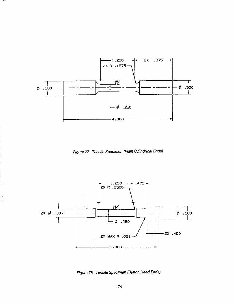
I¢ .5oo --
i
4.000
1.375---"
I--_ .5oo
Figure 77. TensileSpecimen (PlainCylindricalEnds)
I2X _ .307
l
l.250-----," .475
.2500
r----'L ,._, _¢ .z5o
2X MAX R .051
3.000
2X .400
I•500
I
Figure 78. Tensile Specimen (Button Head Ends)
174

The test stand is located at LWI, Applied Technology Division, City of Industry, California. This machine wascalibrated by a certified MTS service engineer on May 28, 1991. All the calibrations were within the range ofASTM standards.
To minimize bending strains, specimen fixtures were aligned such that the major axis of the specimen closelycoincided with the load axis. The maximum bending strain determined was 1 percent of the average axial strain.Five percent is the maximum allowable bending strain per ASTM Standard E466 and E606.
VI.B.5.1v T_Ft Procedure
All the tensile tests were performed in accordance with ASTM Standard B557 and reference standards of ASTMA370 and E8. The broken specimens were inspected and stored for further references. Load control testing ata nominal stress rate of 86 ksi/minute was used, based on the recommendation of ASTM B557, Procedure7.2.7.2. A typical stress-time curve obtained during testing (WE43 magnesium alloy, Specimen #8) is shown in
Figure 79. The actual load and strain data values that made up the stress-strain curves (see Results section)were stored through a PC-based data acquisition system. These data files were used for data reduction andarchived for further studies of the material properties. Twenty-four tests of each material were used to calculateand determine the tensile properties.
VI.B.5.v Results
A typical stress-strain curve (WE43 magnesium alloy, Specimen #8) from the tensile tests is shown in Figure 80.The data summaries for all tests are shown in Tables 64, 65, and 66. There are slight deviations in calculatedmoduli of C355T7 due to the different specimen configuration (shown in Figures 77 and 78). To havecomparative information, only 15 test data (Specimen Nos. 1-15) of C355T7 cylindrical end specimens(Figure 77) were used for statistical analysls. The mean values of yield strength, tensile strength, elongation,and modulus were determined and listed in Tables 68, 69, and 70. The yield strength was determined by the"offset method" at an offset of 0.2 percent from the stress-strain diagrams. The modulus of elasticity wascalculated from the proportional section of the stress-strain curves.
The yield strength, tensile strength, elongation, and the usable high temperatures of these three gear casematerials are compared in Table 71, along with published reference data.
VI.B.5.vi Discussion of Results
WE43, ZE41A, and C355T7 are candidate housing materials for the design of future gearboxes operating atelevated temperatures. As derived from these tests, WE43 is the most ductile material. Also, the tensile strengthof WE43 is similar to C355T7, but the yield strength of WE43 is only about 76 percent that of C355T7.
As shown in Table 71, WE43 has the highest service temperature (up to 572°F). Magnesium alloy also is
approximately two-thirds the weight of aluminum alloy. These are critical factors in the design of advancedhelicopter transmissions.
The tensile tests from this program were conducted at room temperature. For future testing, it is recommendedthat elevated temperature tensile tests be performed to determine mechanical properties at anticipatedoperating temperatures of around 325 to 400°F. The creep properties of these three materials at elevatedtemperatures should also be determined by future tests.
175

TABLE 64. TEST DATA OF WE43
Specimen
No.
1
2
3
4
5
6
7
8
9
10
11
12
13
14
15
16
17
18
19
20
21
22
23
24
Diameter
(in.)
Area
(in. 2)
0.251
0.250
0.251
0.250
0.251
0.250
0.250
0.249
0.250
0.249
0.250
0.249
0.250
0.250
0.250
0.250
0.250
0.249
0.249
0.25O
0.249
0.25O
0.249
0.250
0.0495
0.0491
0.0495
0.0491
O.0495
0.0491
0.0491
0.0487
0.0491
0.0487
0.0491
0.0487
0.0491
0.0491
0.0491
0.0491
0.0491
0.0487
0.0487
0.0491
0.0487
0.0491
0.0487
0.0491
Yield Strength
0.2% Offset
(ksi)
25.7
25.5
28.5
28.1
25.9
25.2
26.0
26.4
29.6
26.0
25.4
27.9
27.9
25.9
28.0
25.9
28.4
25.4
26.0
25.9
25.5
29.3
25.8
25.8
Tensile
Strength
(ksi)
38.8
39.1
42.2
41.6
38.7
36.9
39.3
39.9
43.0
39.2
39.7
41.3
40.9
39.2
38.6
39.7
40.8
39.6
39.2
38.8
40.1
43.1
38.7
38.2
Elongation*
%
9,6
8.3
9.6
7.9
7.1
5.3
7.9
8.3
9.8
8.2
10.1
6.8
7.1
7.9
3.6
8.9
6.4
9.5
8.3
8,7
13.3
8.8
7.9
7.6
Modulus of
Elasticity
(ksi)
6483
6438
6491
6515
6516
6511
6439
6470
6554
6507
6545
6549
6446
6441
6563
6474
6510
6494
6459
6421
6314
6537
6458
6326
*Original gage length = 1 inch
176

TABLE 65. TEST DATA OF ZE41A
SpecimenNo.
1
2
3
4
5
6
7
8
9
10
11
12
13
14
15
16
17
18
19
20
21
22
23
24
Diameter
(in.)
0.250
0.252
0.250
0.253
0.251
0.250
0.250
0.252
0.249
0.250
0.251
0.250
0.250
0.250
0.250
0.251
0.249
0.251
0.250
0.25O
0.25O
0.250
0.250
0.250
Area
(in. 2)
0.0491
0.0499
0.0491
0.0503
0.0495
0.0491
0.0491
0.0499
0.0487
0.0491
0.0495
0.0491
0.0491
0.0491
0.0491
0.0495
0.0487
0.0495
0.0491
0.0491
0.0491
0.0491
0.0491
0.0491
Yield Strength Tensile
0.2% Offset Strength
(ksi) (ksi)
21.4
21.3
21.1
21.4
20.9
21.2
21.3
20.9
32.1
31.4
32.5
32.1
32.5
32.2
32.4
31.5
Elongation*
%
4.6
3.7
5.1
4.6
5.0
4.6
4.9
4.1
20.3
21.4
20.5
20.5
20.7
21.3
21.2
21.0
20.5
20.8
20.9
21.4
20.8
20.9
21.6
21.3
31.5 4.4
31.9 4.2
32.1 5.0
31.6 4.6
32.2 5.0
32.2 4.6
31.9 4.2
31.6 4.2
32.2 4.7
31.8 4.5
32.4 4.9
32.3 4.8
32.0 4.8
31.7 4.5
32.5 5.0
31.9 4.4
Modulus of
Elasticity
(ksi)
6462
6576
6497
6438
6538
6469
6430
6473
6453
6701
6436
6374
6359
6317
6471
6415
6567
6567
6461
6392
6502
6378
6399
6404
*Original gage length = 1 inch
177

TABLE 66. TEST DATA OF C355T7
Specimen
No.
1
2
3
4
5
6
7
8
9
10
11
12
13
14
15
16
17
18
19
20
21
22
23
24
*Original
Diameter
(in.)
0.250
0.252
0.250
0.251
0.251
0.250
0.250
0.251
0.251
0.251
0.25O
0.250
0.249
0.251
0.250
0.252
0.252
0.252
0.252
0.252
0.253
0.253
0.253
0.253
gage length =
Area
(in .2)
0.0491
0.0499
0.0491
0.0495
0.0495
0.0491
0.0491
0.0495
0.0495
0.0495
0.0491
0.0491
0.0487
0.0495
0.0491
0.0499
0.0499
0.0499
0.0499
0.0499
0.0503
0.0503
0.0503
0.0503
linch
Yield Strength0.2% Offset
(ksi)
33.8
35.7
35.4
35.4
36.2
35.6
35.3
35.3
35.2
34.0
35.3
35.6
33.0
35.3
35.3
36.3
36.7
34.2
36.0
37.1
34.4
34.7
36.2
34.6
Tensile
Strength
(ksi)
39.6
42.5
40.7
42.4
43.4
42.0
41.7
41.7
42.4
41.3
42.0
39.8
39.4
40.3
40.3
44.0
43.6
41.0
40.2
45.2
40.5
41.1
42.9
43.0
Elongation*%
2.1
3.1
2.0
3.5
3.3
2.5
2.5
2.7
3.2
3.0
2.9
2.0
2.3
2.0
2.0
4.5
3.6
2.9
2.0
5.0
2.3
2.5
3.0
5.9
Modulus of
Elasticity
(ksi)
10589
10776
10619
10427
10604
10888
10498
10765
10479
10854
10577
10495
10581
10660
10762
11246
11651
11610
12048
12667
12295
12203
11986
11781
TABLE 67. HEAT TREATMENTS AND HARDNESS
Material
Magnesium Alloy ZE41A
(Condition T5)
Magnesium Alloy WE43
(Condition T6)
Atuminum AUoy C355T7
(Condition TT)
Solution Heat
Treatment
2 hrs at 626°F, cool in air
8 hrs at977°F, hot water
quench at140°F-176°F
12 h_ at980°F, water
quench at 70°F
Aging
Treatment
16 hrs at 356°F
16 hrs at 482°F
8 hrs at 440°F
Hardness
BHN 60
BHN 71
BHN 81
i!i 178

5O000
ZSO00
Sample WE43 _ 8
i
_fpP
I I0,00 25.0
TIME ISocl
50.0
Figure 79. WE43 Stress-Time Curve
5o0oo
Sample WE43 J 8
sTRESS
PS
i
37500
_3000
0 I I I
0.00 0.00 0.00 0,00 0.00
STRAIN (Inllnl
Figure 80. WE43 Stress-Strain Curve
179
q-5
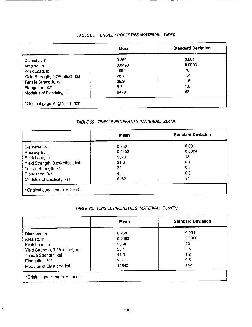
TABLE 68. TENSILE PROPERTIES (MATERIAL: WE43)
Diameter, In.
Area sq, in.Peak Load, Ib
Yield Strength, 0.2% offset, ksiTensile Strength, ksiElongation, %*Modulus of Elasticity, ksl
Mean
0.250
0.0490195426.739.98.26478
Standard Deviation
0.0010.0003
761.41.5
1.863
*Original gage length = 1 inch
TABLE 69. TENSILE PROPERTIES (MATERIAL: ZE41,4)
Diameter, in.
Area sq, in.Peak Load, lb
Yield Strength, 0.2% offset, ksiTensile Strength, ksi
Elongation, %*Modulus of Elasticity, ksi
Mean
0.2500.0492157621.032
4.66462
Standard Deviation
0.0010.0004180.40.30.3
84
*Original gage length = 1 inch
TABLE 70. TENSILE PROPERTIES (MATERIAL: C355T7)
Diameter, in.
Area sq, in.Peak Load, Ib
Yield Strength, 0.2% offset, ksiTensile Strength, ksi
Elongation, %*Modulus of Elasticity, ksi
Mean
0.2500.0493
203435.141.32.5
10640
Standard Deviation
0.0010.0003680.81.20.6142
*Original gage length = 1 inch
18O

TABLE 71. TENSILE TEST RESULTS SUMMARY
Material
WE 43
ZE41A
C355T7
Yield Strength
0.2% Offset, ksi
26.7
(26.8 average)
21.0
(22.6 average)
35.1
(35.0 min.)
Tensile Strength
ksi
39.9
(38.4 average)
32.0
(29.0 average)
41.3
(38.0 min.)
Elongation%
8.2
(7.0 average)
4.6
(3.0 average)
2.5
(2.0 rain.)
Usable High
Temperature*
572°F
320°F
400°F
( ) Published reference data are shown In parenthesis.
*Usable high temperatures and reference data of WE43 and ZE41A were suggested by Magnesium Elektron,
Inc., and 400°F service temperature and reference data of C355T7 was from Lucas Western Specification
MPS 49500B415.
VI.B.6 Face Gear Capacity Tests
VI.B.6.i Introduction
Experimental tests on face gears were performed in the NASA Lewls spiral bevel gear rig (Handschuh, et al.,
1992) [63]. The face gears tested, shown in Figure 81, were basically a half-size version of the MDHC/Lucas
ART design. The gears were 16 pitch with 28 teeth on the pinion and 107 teeth on the face gear. The shaft
angle was 90 degrees to accommodate the rig.
VI.B.6.ii Test Article DeF¢ription
A limited amount of test gears were available for test (four pinions and four face gears). The gears were made of
Maraging 300 steel per AMS 6514. The pinions were nitrided and ground with a case hardness of Rc 58. The
face gears were shaper cut and hardened to Rc 52. A method for grinding face gears has not been developed
yet, although this is the subject of an additional MDHC/LWl IR&D program currently underway.
181

Figure 81. Gears Installed in Test Stand
Vi.B.6.iii Test Rig Description
The NASA-Lewis spiral bevel gear rig, shown in Figure 82, operates on a closed loop or torque-regenerativeprinciple. Two sets of pinion/face gears are used in the loop with the two pinions connected by a cross shaft.The outputs of the two face gears are connected through a helical gear mesh. A hydraulic loading system isconnected to the helical mesh which puts a thrust load on the mesh, and thus, the torque in the loop. A variablespeed motor is connected by a belt to the loop and powers the test stand.
VI.B.6.iv Test Procedure
The objective of the tests was to demonstrate the feasibility of face gears and determine the failure modes forhigh power applications. For the tests, 100-percent design speed and torque were defined as 19,000 rpm pinion
speed and 68 N-m (600 in.-Ib) pinion torque for a power of 135 kW (180 HP). The gears were run at 74°C(165°F) oil inlet temperature using an ample supply of DOD-L-85734 lubricant at about 0.8 gpm per mesh.
VI.B.6.v Results
Four sets of gears successfully completed 26-hour (30x106 pinion cycles) endurance runs at 100 percent speedand torque. The contact pattern on the teeth was good and developed on the full tooth of the face gear. Thepinion teeth showed normal wear. The face gear teeth, however, had some surface distress. The teeth from thetest side (pinion driving the face gear) had moderate wear and were in good condition. The teeth from the slave
side (face gear driving the pinion) had small pit lines in some instances in the middle region of the teeth.
The gears were subsequently run 26 hours at 200-percent torque and 100-percent speed. One test (two sets ofgears) lasted the 26 hours with the pinions showing moderate wear and the face gears showing increasing
surface distress. The second test (the additional two sets of gears) was suspended after about 10.5 hours due
182

to a tooth breakage on one of the face gears (slave side). The breakage originated from the surface pit line fromthe previous test.
VI.B.6.vi Discussion of Results
The results, although limited, demonstrated the feasibility of face gears in high-speed, high-load applications.The tests did show surface distress with the face gears, however. The use of a hardened, ground gear steel (inuse for conventional aircraft gears today but not presently available for face gears since manufacturingtechniques do not exist to grind face gears) would significantly increase the surface durability and make facegears available for high-power application.
Figure 82. NASA Spiral Bevel Gear Rig
183

VII. SUMMARY OF RESULTS - CONCLUDING REMARKS
The McDonnell Douglas Helicopter Company (MDHC) and teammate Lucas Western, Inc. (LWI) have completedthe design of a 5000-horsepower Advanced Rotorcraft Transmission (ART) within Phase I of the Army/Nasa ART
Program. The Innovative split torque configuration using face gears has met or exceeded the Army/NASAweight, noise and reliability goals set for the program. In working to achieve the goals, transmission design andanalysis processes were performed interactively to attain the desired design characteristics.
The weight goal for the ART Program was to attain a 25 percent weight reduction for the 5000 HP transmissionrelative to a state-of-the-art (SOA) baseline design. A 5000 HP upscaled Apache main transmission served asthe $OA baseline transmission for goal progress comparisons. The MDHC/LWl ART design, weighing 815 Ib,
reached a 40 percent weight reduction relative to the 1347 Ib SOA baseline transmission weight. This was 195Ib below the 1010 lb goal, and was achieved through use of the novel split torque configuration, an optimizedcombination of gear ratios, and weight-conscious design of Individual components. The use of face gears In theART first stage was found to be a significant weight and space savings development. Face gear geometryallows torque splitting from a single Input pinion, with second stage torque recombination then occurringdirectly, as all second stage pinions rotate In the same direction and in a single plane above. Implementation ofthe high contact ratio planetary provided additional weight reduction, as did the detail design of the ARTtransmission subsystems. The positive engagement overrunning clutch yielded a weight-competitive designhaving enhanced reliability characteristics and reduced cooling requirements. The advanced lubrication systemdecreased the transmission installation weight. A lightweight secondary lubrication system employing low flowrate oll misters provides oil for more than one hour of emergency operation.
The ART program reliability goal was 5000 hours Mean-Time.Between-Removal (MTBR). The split torque ARTtransmission was analyzed during the design process to achieve this goal. Reliability requirements wereapportioned to the transmission component level. This was done both for dynamic components and for thosewhich could contribute to miscellaneous failures. Loading and cycling of individual dynamic components wereevaluated to attain at least the 14,100-hour component lives required to yield the 5000-hour system life. In
addition, other components which affect removal intervals such as seals and housing sections were designed tooperate for the duration of their required lives. The MTBR obtained for the ART transmission as a result of the
design and analysis processes is 6269 hours, exceeding the 5000-hour goal.
The ART program noise goal was to reduce source noise by 10 dB relative to a 5000 HP SOA baseline
transmission. The noise level identified as meeting this goal by the MDHC/LWl team was 97.9 riB. This is 10 dBbelow the 107.9 dB noise level obtained from the upscaled 5000 HP Apache baseline transmission. The 107.9dB noise level was based on extrapolated Apache transmission test data. The predicted source noise level forthe ART is 98.3 riB, which is 9.6 dB below the 107.9 dB SOA noise level, essentially meeting the goal. In workingto achieve the 10 dB reduction, gear web, rim and shaft deflections were analyzed during the design process tominimize noise. The transmission housing structural shape, ribs and stiffeners were designed to minimizevibratory deflections. Also, the high contact ratio (HCR) dropped-tooth planetary was implemented mainly tofacilitate noise reduction. The planetary design, in addition to having HCR tooth modifications, Incorporates
tooth phasing methods and a cantilevered ring gear in minimizing noise. Use of nonstandard tooth proportionsIn the second stage gear designs also contributed to noise reduction.
Significant aircraft mission performance Improvements and cost savings are realized from use of the ART
transmission. The improvement in loss-exchange ratio during combat is 17 to 22 percent. A 12 percentimprovement is seen in the ability to sustain a given level of combat operations. The Mean-Time-Between-
184
Failure (MTBF) increase represents a 22 percent Improvement. Use of the ART would also result in atransmission acquisition cost savings of 23 percent or $165K, per unit. An average transmission directoperating cost savings of 33 percent, or $24 per flight hour, would also be realized.
The ART three-stage split torque design with face gears offers several areas for future investigation which shouldyield substantial technology gains. Of primary interest is the first and second stage split torque section of thetransmission. Proof-of-concept split torque tests were initiated by the MDHC/LWI team in late 1992. Usingresults of these tests as a guide, follow-on design, fabrication and testing will be proposed to refine the conceptand maximize its potential. Also, the need to perform additional face gear capacity tests in conjunction with the
above is apparent, and such tests with ground face gears are planned. Face gear grinding technologydevelopment is currently underway. Another effort will evaluate transmission configurations for uses in futurehigher horsepower versions of the Apache. A two-stage ART transmission design, having only the two splittorque stages, will be compared with designs of the three stage ART and a configuration similarto the existing2828 HP Apache transmission. The evaluations will compare the designs on the basis of the U.S. Army weight,noise and reliability goals, as well as mission effectiveness, flight performance and cost parameters.
Follow-up work should be performed on other portions of the ART Phase I design as well. The proposedrotorcraft application of a pawl and ratchet-based positive engagement clutch merits a detail design, fabricationand test program to compare this to existing rotorcraft clutch designs. The high contact ratio planetary,Implemented as the third stage of the Phase I ART design, is worthy of fabrication, evaluation testing andcomparison with standard planetary designs. Such planetary tests should be performed In conjunction with anacoustic modeling effort to investigate correlation of actual versus predicted noise levels.
The MDHC/LW1 ART offers considerable improvements to SOA rotorcraft transmisslon design. Substantialprogress was made in meeting or exceeding the U.S. Army/NASA weight, noise and reliability goals. The threestage split torque single planetary transmission can provide significantly increased capabilities for a fieldedaircraft.
185

APPENDIX A
POSITIVE ENGAGEMENT CLUTCH ANALYSIS
Theanalysissectionbelow covers curvlc coupling stress analysis, helical spllne stress analysis, resonant
frequency analysis, pawl balance calculation, hydroplanlng analysis, spring stress analysis, and engagementsystem analysis. Individual clutch components are illustrated In Figure 4 of the Transmission Configurationsection.
CURV,IC COUPLING STRESS ANALYSIS
Curvlc coupling stress analysis is based on the Gleason system:
where,
D = 3 -k//'T'/1,310
D is the coupling outside diameterT Is ultimate torque In In.-Ib
Face length is 0.125 x outside diameter and material ultimate strength is 150,000 psi. The design uses a 2.0 Inchoutside diameter, 0.25 inch face length and 9310 steel with an ultimate strength of 250,000 psi. The ultimateallowable torque is:
23 x 1,310 x 250,000/150,000 = 17,467 psi
Maximum continuous applied torque Is:
63,025 x 3,000 HP/20,950 rpm = 9,025 in.-Ib
Ultimate torque is:
1.5 x 9,025 = 13,538 in.-Ib
Margin of Safety (M. S.) is:
17,467/13,538- 1 = +0.3
HELICAL SPLINE STRESS ANALYSIS
The helical spline is 8/16 pitch, 17 teeth and 45-degree helix angle, one half of the teeth carry load.
Shear stress is:
8T/_r D2 F (sin _) = 8 x 9,025/7r x 2.1252 x i x 0.707 = 7,200 psi
M. S. = Large
186

CompressivestressIs:
2T/DNF(sin_,)= 2x 9,025/2.125x 17x 1x0.707= 706.7pslM.S.= Large
RESONANT FREQUENCY ANALYSIS
This section contains the natural frequency analysis of the pawl about its center of rotation. The polar massmoment of inertia of the pawl was calculated by the integration of 16 element sections, see Figure 83 and Table72. A helical tension spring was sized for 31 Ib/in. The spring rate is easily modified by changing any or all ofthree variables: wire diameter, coil diameter, and number of coils. Thus, the optimum spring rate can be foundreadily by experiment.
Spring rate is:
K = G d4/8D 3 N
where,
G is Modulus of Rigidity = 11,500,000 psi
d is Wire diameter = 0.035 inch
D is Coil mean diameter = 0.325 inch
N is Number of coils = 2 coils/pawl
Figure 83. Section Integrated System Used to Calculate Polar Mass Moment of Inertia
and Centrifugal Force Moment of Pawl
187

TABLE 72. PAWL POLAR MASS MOMENT OF INERTIA, J
Element
No.
I
2
3
4
5
6
7
8
9
10
11
12
13
14
15
16
Hole
t
Thickness
(inch)
0.20
0.20
0.20
0.20
0.20
0.20
0.20
0.20
0.20
0.2O
0.2O
0.2O
0.20
0.20
0.20
0.2O
0.20
A
Area
(inch 2)
0.055 x 0.050
0.05 x 0.110
0.05 x 0.157
0.05 x 0.210
0.05 x 0.255
0.05 x 0.260
0.05 x 0.275
0.05 x 0.295
0.05 x 0.300
0.05 x 0.260
0.05 x 0.215
0.05 x 0.200
0.05 x 0.205
0.05 x 0.195
0.05 x 0.095
0.02 x 0.030
7r/4 (0.11) 2
r
Radius
(inch)
0.375
0.333
0.285
0.240
0.315
0.133
0.078
0.025
0.025
0.078
0.133
0.208
0.295
0.385
0.450
0.480
0.213
tAr 2
(inch 5)
77.34 x 10⁶
121.98
127.52
120.96
253.02
45.99
16.73
1.84
1.88
15.82
38.03
86.53
178.40
289.04
192.38
27.65
-86.23
1,508.9
J = (0.0015089 inch 5) (0.283 lb/in3)/386.05 in/sec 2 = 1.105 x 10 -6 Ib-ln-sec 2
Thus,
K = 11,500,000 x (0.035)4/8 x (0.325) 3 x 2 = 31 Ib/in
Resonant frequency is:
W = "_/'_/J
where a Is the distance from spring line of action to pawl pivot = 0.368 inch
W = [ 31 x (0.368)2/1.105 x 10 -6 ]1/2
W = 1,948 radians/second
f = 1,948/27r = 310 Hertz
188

PAWL BALANCE CALCULATIONS
The pawl moment due to centrifugal forces has been calculated by integrating section elements of pawl mass.
The sectioning is as shown on Figure 83. The clockwise and counter clockwise section moments are given in
Table 73 where I is the distance from the clutch rotational axis to the center of gravity of each sectional element
and r is the distance from the pawl rotational axis to the center of gravity of each sectional element.
TABLE 73. PAWL CLOCKWISE AND COUNTERCLOCKWISE SECTION MOMENTS
Element
No.
t
Thickness
(inch)
I
Length
(inch)
A
Area
(inch 2)
Clockwise
r
Radius
(inch)
tlAr
(inch 5)
1
2
3
4
5
6
7
8
0.20
0.20
0.20
0.20
0.20
0.20
0.20
0.20
0.583
0.555
0.530
0.503
0.473
0.428
0.398
0.385
0.055 x 0.050
0.05 x 0.110
0.05 x 0.157
0.05 x 0.210
0.05 x 0.255
0.05 x 0.260
0.05 x 0.275
0.05 x 0.295
Hole
9
10
11
12
13
14
15
16
0.20 0.500 7r//4 (0.11)2
Counterclockwise
0.20
0.20
0.20
0.20
0.20
0.20
0.20
0.20
0.385
0.380
0.373
0.333
0.295
0.294
0.330
0.358
0.05 x 0.300
0.05 x 0.267
0.05 x 0.215
0.05 x 0.200
0.05 x 0.205
0.05 x 0.195
0.05 X 0.095
0.05 X 0.030
0.375
0.333
0.285
0.240
0.315
0.133
0.078
0.025
0.215
0.025
0.078
0.133
0.208
0.295
0.385
0.450
0.480
120.24 x 10 -6
203.30
237.15
253.51
379.94
148.OO
85.37
28.39
1,455.90
-204.32
28.87
79.14
106.66
138.53
178.40
220.72
141.08
20.62
914.02
Q = ]_ (tl A r) e/g (27r/60) 2 (RPM) 2
= (1455.90- 204.32- 914.02) (.283/386.04) (2_r/60) 2 (20950) 2 (10)-6
= 1.191 in-lb clockwise (nose down)
189
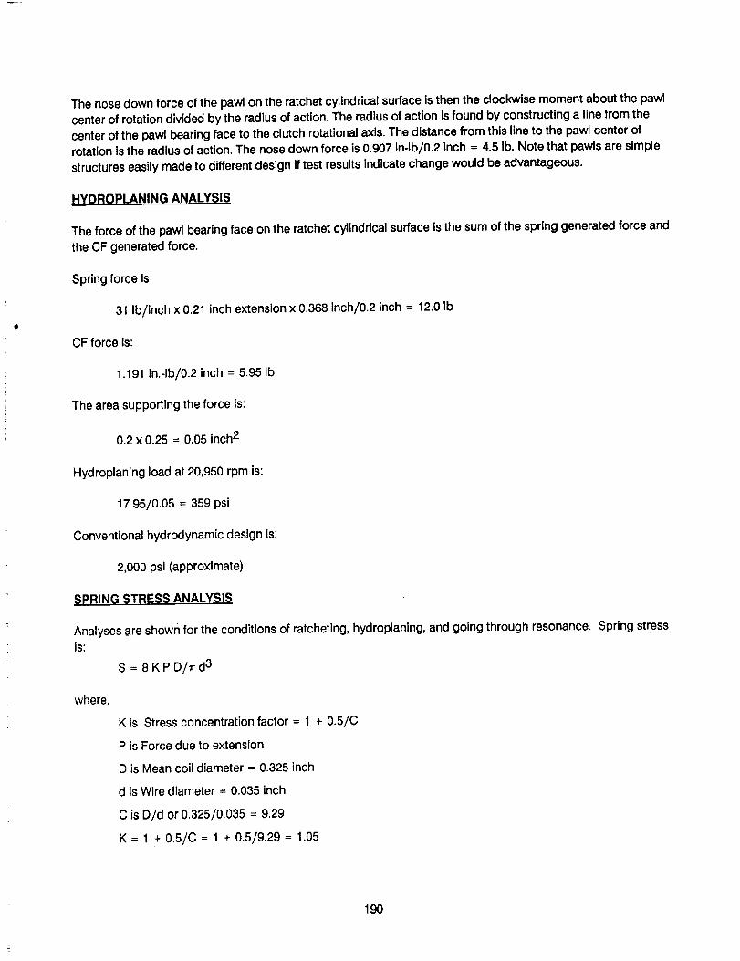
The nose down force of the pawl on the ratchet cylindrical surface is then the clockwise moment about the pawlcenter of rotation divided by the radius of action. The radius of action is found by constructing a line from thecenter of the pawl bearing face to the clutch rotational axis. The distance from this line to the pawl center ofrotation Is the radius of action. The nose down force is 0.907 ln-lb/0.2 inch = 4.5 lb. Note that pawls are simple
structures easily made to different design if test results Indicate change would be advantageous.
HYDROPLANING ANALYSIS
The force of the pawl bearing face on the ratchet cylindrical surface isthe sum of the spring generated force andthe CF generated force.
Spring force Is:
31 Ib/inch x 0.21 inch extension x 0.368 inch/0.2 inch = 12.0 Ib
CF force is:
1.191 in.-Ib/0.2 inch = 5.95 Ib
The area supporting the force is"
0.2 x 0.25 = 0.05 inch 2
Hydroplaning load at 20,950 rpm is:
17.95/0.05 = 359 psi
Conventional hydrodynamic design Is:
2,000 psi (approximate)
SPRING STRESS ANALYSIS
Analyses are shown for the conditions of ratcheting, hydropianlng, and going through resonance. Spring stressis:
S=8KPD/Trd 3
where,
K is Stress concentration factor = 1 + 0.5/C
P is Force due to extension
D is Mean coil diameter = 0.325 inch
d is Wire diameter = 0.035 inch
C is Did or 0.325/0.035 = 9.29
K = 1 + 0.5/C = 1 + 0.5/9.29 = 1.05
190

During:
Ratcheting:
Hydroplaning:
Resonance:
Ratcheting:
Hydroplaning:
Resonance:
P = 0.08inchx 31Ib/inch= 2.48Ib
P = 0.21inchx 31Ib/inch= 6.51Ib
P= 0.24inchx 31Ib/inch= 7.44Ib
S = 8x 1.05x 2.48x 0.325/7rx 0.0353= 50,264psi
S = 8x 1.05x 6.51x 0.325/7rx 0.0353= 131,944psi
S= 8x 1.05x 7.44x 0.325/_rx 0.0353= 150,793psiSult = 250,000psiM.S.= 250,000/150,793x 1.5- 1= 0.10
ENGAGEMENT SYSTEM ANALYSIS
Pawl System
The pawl system of the positive engagement clutch provides the means for sensing the proper instant to initiateengagement and for operating the synchronizer to complete the engagement. It Is essential that theengagement operation commence as soon as Input speed has overtaken output speed and the face spline teethare in alignment.
in the subject clutch, positive pawl system operation is assured by avoidance of pawl resonance during the timeinterval immediately preceding engagement.
The second design element required to assure reliable pawI system operation Involves minimizing wear and
fatigue of the pawl-ratchet system in long-term overrunning. By promoting pawl hydroplaning at all continuousoverrunning conditions, metal-to-metal wear between pawls and ratchet teeth can be avoided and return springcyclic motion minimized.
Figure 84 Is a plot of pawl action versus differential input to output speed. By assuming uniform acceleration ofthe input from zero to full speed in 5 seconds, a scale of time to go to synchronous speed can be added to theabscissa; and by knowing the number of teeth in the ratchet, ratchet tooth exciting frequency can be added tothe ordinate.
As the plot indicates, pawl system behavior passes through three distinct phases as differential speed changes:
1. Pawl hydroplaning, wherein differential speed between the pawls and the oil annulus carried in theratchet is sufficient to support the pawl hydrodynamically.
2, Resonant behavior, where the speed differential will no longer support hydroplaning, so that thepawls become propelled by the ratchet teeth. When the ratchet pulses occur at the frequency whichthe pawls are unable to follow, then the pawls will tend to bounce at their natural frequency. A pinstop is provided to limit resonant excursions.
. Coherent pawl and ratchet interaction occurs when the ratchet passage frequency becomes lessthan the pawl natural frequency and each pawl falls into each ratchet pocket as it comes by.
191

2_0 _0
=E 200O0a.
n..!
|15000
_. 10000
5000
2000_D
-1-m
_r 1500L..
LL
8
iooo
\
\Pawl Hydroplaning
500 _._ Pawl310
k /
-Hz=5-419T
\\
r,
Resonance Zone
tCoherent Pawl/Ratchet Action
0 0 r I I ......I4 3 2
Time To Synchronization - Seconds
5
Tf_
1/fn
Figure 84. Paw/Behavior vs. Differential Input to Output Speed
The main thrust of pawl system design Is to exercise control over the extent of these zones to promote reliable
operation and long life.
The highest predicted natural frequency is 310 hertz while the shaft operating speed is 350 hertz. This proximityis not a cause for concern based on the foliowlng considerations:
Clutch Enaaaed
The pawl In the ratchet notch Is submerged in the oil annulus formed by dams at either end of the ratchet. Theoil annulus will resist displacement. There isfriction at the pawl pivot which resists motion. The distance from the
pawl tip to the ratchet face is the distance generated by the slope of the curvic coupling teeth in backing thepawl out of contact with the ratchet face. Any oscillation of the pawl would require alternately squeezing an oilfilm out from the radial face or the tangential face of the ratchet while the pawl moves a very small distance.
Clutch Overrunning
The design intent is that the pawls hydroplane on the cylindrical faces of the ratchet while overrunning. Themargin shown is believed satisfactory. If resonant behavior is observed, it Is a very slmple matter to change the
spring or the mass of the pawls.
192

Determination Of Ability Of Pawl To Enaaae Ratchet In The Available Tim.n
In the ART drive system, it is possible for the speed differential between input and output to change rapidly as an
engine accelerates up to engagement speed. It is assumed that this acceleration rate can be as high as 0 to
20,950 rpm in 5 seconds.
The plot given in Figure 81 shows that the input to output speed differential diminishes as the instant of
synchronization (To) approaches. The rate of change of differential speed is:
20,950 rpm/5 seconds = 4,190 rpm/sec
Converting to rev/sec 2 results in:
4,190/60 = 69.8 rev/sec 2
Since there are 6 teeth in the ratchet, the rate of change of ratchet tooth exciting frequency is:
6 x 69.8 Hz thus,
ft = 419 impacts/sec 2 (1)
where,
ft = Ratchet tooth exciting frequency
Working back from the Instant of synchronization (To), we can say that the last resonant pawl cycle must be
completed at TO or sooner. It can also be seen that the last opportunity for the start of that resonant cycle
occurs when the ratchet tooth exciting frequency, ft, just equals the pawl natural frequency, fn-
The period of time for one resonant cycle is:
1/fn
From (1), the time preceding To for ft to equal fn is:
fn/419
As a minimum, let:
1/f n = fn/419
Therefore,
fn = _ =20.47Hz
193

For a rotationally vibrating system,
= 1/2_r -kK/'_/Jfn
where,
Thus,
and,
Ks = Spring rate of pawl return spring, Ib-ln./rad
J = Pawl polar mass moment of Inertia = 1.105 x 10⁻⁶ Ib-ln. sec2
20.47 = 1/2_'"_Ks/1.105 x 10-6
Ks = 0.0183 Ib-in./radian
Note that this a minimum; any spring rate exceeding this value Is satisfactory.
Spring force is:
31 Ib/in x 0.21 extension = 6.51 Ib
Spring Torque is :
6.51 Ib x 0.368 inch from spring centerline to pawl pivot = 2.40 in-lb
Applied Angle Is:
20 ° rotation to engage ratchet = 0.349 radians
Actual Ks is:
2.40 x 0.349 = 0.84 Ib-in./radianM. S. = Large
194
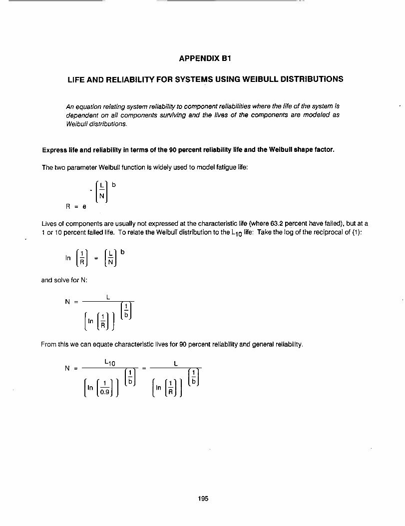
APPENDIX B1
LIFE AND RELIABILITY FOR SYSTEMS USING WEIBULL DISTRIBUTIONS
An equation relating system reliability to component reliabilities where the life of the system is
dependent on all components surviving and the lives of the components are modeled as
Weibull distributions.
Express life and reliability in terms of the g0 percent reliability life and the Weibull shape factor.
The two parameter Weibull function Is widely used to model fatigue life:
MoR = e
Lives of components are usually not expressed at the characteristic life (where 63.2 percent have failed), but at a
1 or 10 percent failed life. To relate the Weibull distribution to the L10 life: Take the log of the reciprocal of (1):
and solve for N:
N m
L
From this we can equate characteristic lives for 90 percent reliability and general reliability.
N
L10 L
[In /0---_] I [b] [In [1]] [b]
195
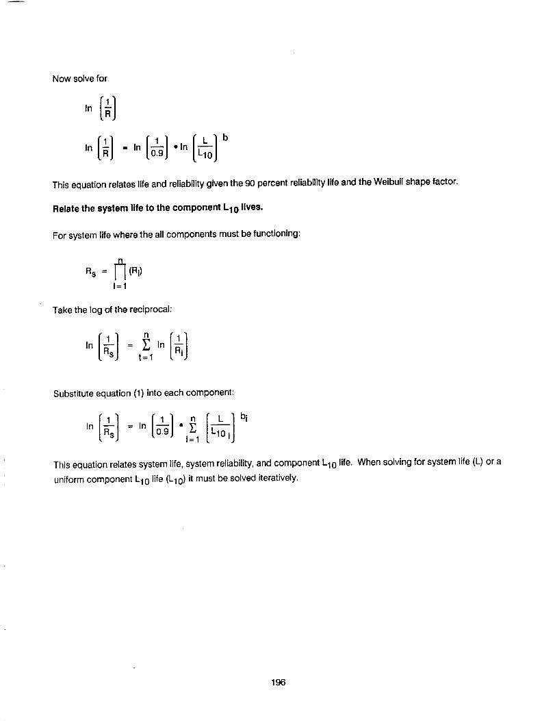
Now solve for
oHoI l;,oI l-,o[L+01
This equation relates life and reliability given the 90 percent reliability life and the Weibull shape factor.
Relate the system life to the component LIO lives.
For system life where the all components must be functioning:
Rs = _'_ (Ri)
i=1
Take the log of the reciprocal:
In 1 = _ Int=l
Substitute equation (1) into each component:
In [_ss] = In I01-_] "i=1_ [ L_Oi] bi
This equation relates system life, system reliability, and component LIO life. When solving for system life (L) or a
uniform component L10 life (L10) it must be solved iteratively.
196

APPENDIX B2
FAILURE MODES EFFECTS AND CRITICALITY ANALYSIS (FMECA)
This section is provided as the basis of a full-scale FMECA for the production phase of the ART.
A FMECA consists of 2 parts:
1. Failure mode and effects analysis (FMEA)
2. Criticality Analysis
This section will present FMECA data in Table 74.
FMECA includes the preceding reliability analysis as a prelude to filling out the tables. The FMECA spec (MIL-STD-1629A) calls out activities (a-h) which support the design process including:
.
2.
.
.
System definition. Completed by design with input from specialists.
Block diaqrams. These diagrams, shown in Figure 85 are presented in a hierarchy, reflecting how
reliability was apportioned and analyzed.
Interface failure modes. The integration of the system is an Important part of the ART task. MDHChas considered all potential interfaces to the extent possible I.e. there is no FAAV design available
for reference. When the pre-production verslon of the ship drawings become available, this effortcan be completed.
Severity cla,s_ification. Used to provide a qualitative measure of the worst potential consequencesresulting from design error or item failure.
a. Cateqory I - Catastrophic. A failure which may cause death or loss of ship.
b. Cateqory II - Critica!. A failure which may cause severe Injury, major property damage, ormajor system damage resulting in misslon abort.
c. Cateqory III - M_rqinal. A failure which may cause minor injury, minor property damage, orminor system damage which results In delay of loss of availability or mission degradation.
d. Cateaory IV- Minor. A failure not serious enough to cause Injury, property damage, orsystem damage, but will result in unscheduled maintenance action.
e. Failure detection methods are Identified in the table.
f. Corrective actions
Ib
197

TABLE 74. FAILURE MODES, EFFECTS AND CRITICALITY ANAL YSIS
Part IDand
Function
ART assembly -
Transmit torque tomain rotor
ART assembly -
Transmit torque toaccy. and NOTAR
system
ART Assembly -Allow the rotor
system to overrun
the engine
ART gears,bearings, shafts,
flanges, andsplines -transmit and
change torque
Failure
Modes
Torque Is
not
transmitted
Torque is
partiallytransmitted
Excessive
noise/vibration
Excessiveheat
Methodof
Detection
Visual, flight;characteristics,Instrumentation
Rightcharacteristics,Instrumentation
Audible, vibration,
chip detectors
Oil Temperatureindication.
Failure Effect
Subsystem
Inoperative
Degradedfunction
Failure ofvibration-
sensitive sensorsand electronics.
Reduced life, oil
composition
damaged •
Failure Effect
Nr Vehicle
Safety of Right
Safety of Right -condition of
vehicle becomesOEI
Other system
damagepossible.
none
Seizure Main rotor stops System Safety of Rightcatastrophicfailure
Visual, flight Inoperativecharacteristics,Instrumentation
Audible, vibration,
chip detectors
Torque is
not
transmitted
Excessive
noise/vibration
Excessive
heat
Seizure
:Failure of
vibration-sensitive sensors
iand electronics.
Reduced life, oil
composition
damagedLoss of Anti-
Torque
Overrunningclutch failure
Loss of power tomain rotor
and/oraocy/NOTAR
Rotor
systemlocked to
engineStructural
failure
Oil Temperatureindication.
Tail rotor stops
Main rotor and
engine speedindications locked
together.
Vibration, loss of
power
Safety of Right -Loss of anti-
torquePossible forced
landing
Other system
damagepossible.
none
Safety of Right -Loss of anti-
torquePossible forced
landingReduced
autorotation
capability
Safety of Right
Maximum
Severity,
Compensating
provisions
I, Autorotation
forcedlanding
II,Reduced powerimmediate
landing (30 minute
OEI designed in)I, Non-vibrationhardened
equipment couldbe induced to fail:effect unknown.
III, The ART is
designed to run 30
minutes w/o oil.I, The ART is
designed to run 30
minutes w/o oil.
I, In forward flight,anti-torque is
supplementedwith tail-boom
drag.I, Non-vibrationhardened
equipment couldbe induced to fail:effect unknown.
III, The ART is
designed to run 30
minutes w/o oil.
I, In forward flight,anti-torque is
supplementedwith tail-boom
drag.IV, In autorotationthe rotor will be
driving addt'l mass
I. Highest loadswith Margin ofiSafety used instress calculations
Probability/Data
Source 1!I
< 4/10,000 during30 minute OEI
condition / AGMAstandards
< 1/10,000 over15,000 hour life of
transmission /AGMA standards
Extremely unlikely.
Helicopter
components
generallydesignedto 200 Gs.
Unlikely / Apachefield Ops / Maint
experience0 / No Apachetransmissionseizures to date.
< 1/10,000 duringOEI condition /AGMA gear
bending failurecalculations
Extremely unlikely.
Helicoptercomponents
generally designecto 200 Gs.
Unlikely / Apache
field Ops/Maintexperience
0 / No Apachetransmissionseizures to date.
no data
O/No Apache
structuralfailures
todate.
198

TABLE 74. FAILURE MODES, EFFECTS AND CRITICALITY ANAL YSlS (Continued)
Part ID
and
Function
Over-runningClutch -
Allows rotor to
over-run engine,
transmits torque
Housing -Provides structural
support and
torque reaction
Housing -Retains oil
;Seals - preventcontamination of
gearbox
Seals - prevent oil
from leaking
Primary lubesystem -
provide oil togears and
bearings forlubrication
NOTES:
Failure
Modes
Excessive
gear andbearing
wear-pitting
and spallin_]Unable to
engage
Unable to
disengage
Structuralfailure
Corrosion
iGasket leak
Allowexternal
contaminants to enter
gearboxAllow oil to
leak
Does not3rovide oil to
gears andbearings
Method
of
Detection
Quantitative DebrisMonitor indication
Engine speedindication greater
than rotor speedindication
iEngine and Rotor
speed the samewhen collective
droppedExcessive
Vibration
Visual, QDM
Visible, hi temp,
low oil pressure ifexcessive,
QDM, Oil sample
)oor, oil leakage
reduced oil level,
visual, smell
Pressure and
Temperatureindicators
Failure Effect
SubsystemExcessive noise
and vibration
Cannot transmit
torque.
Unable to
disengage
Cracking,breaking
Reduced life
Loss of oil
Corrosion of
internal parts,excessive wear
none
Increased
friction resultingin higher heat
output
Failure Effect
Nr Vehicle
Excessive noiseand vibration
Possible loss ofmission.
System goes toOEI condition
Reduced
autorotation
capability
Excessive
vibration, loss offunction
vibration, noise,Increases
maintenance
requirements,reduces life
Oil out operation
vibration, noise,Increases
maintenance
requirements,reduces life
Oil buildup onexternal surfaces
Reduced life
Maximum
Severity,Compensating
provisions
IVI QDM will signalwell in advance of
critical problems
IlL 2 engineredundancy.
III. Autorotation nota norma
procedure
I. No Safety offlight relatedfailures to date
IV. Fine filtration
removes particles
IV. ART designedfor 30 rain oil out
operation.IV. Fine filtration
removes particles,Desiccant breather
removes moisture
IV. Dual seal
design
IV. Auxiliary lube
system providesback-up
Probability/Data
Source (1)This mode
calculated in_revious section.
no data
3.72 E-5 / ApacheUMSDC(2) failuredata
2.9 E-5 / ARTmaintainabilityanalysis
0/No Apachefailures
o / ARTmaintainabilityanalysis
1.74 E-5 / ARTmaintainability
analysis
2.9 E-5 1 ARTmaintainabilityanalysis
(1) This is a summary. Please see preceding sections for analysis and basis.
(2) UMSDC is Unscheduled Maintenance Data Collection
199

a. ART Assembly
DynamicComponents(bearings,gears,clutches)
Non-DynamicComponents(seals,housings,lube system,etc.)
%. J
b. ART Dynamic Components
t Clutches
Bearings Gears (two(All (All gearsbearings clutchesin series) in series) in series)
c. ART Non-Dynamic Components
Housing _-_ Lybte m H Seals _-
d. ART Lube System
/,__ Primary Lubrication System| Auxiliary Lubrication System
J
Left
Input
IRightInput
e. ART Seals
• Upper
Static
Mast m
O-Ring
, Lower ,
MainRotorOutput
NOTAR/AccessoryOutput
Figure 85. ART Reliability Block Diagrams
2OO

g. Effects of corrective actions: As the reliability specialist took part in the many design reviews,corrective actions were continuous and preempted erroneous design commitments. Specificexamples Include:
(1) Dynamic component L10 life design goals.
(2) Transmission failure type and frequency probability history.
(3) Reliability suggestions to design Including those described in the maintainabilitysection.
h. Residual problems are documented along with special controls which are necessary to reducefailure risk.
The risk items remaining are:
. The ratchet-and-pawl clutch, in that it has not been used In a helicopter design. Reliabilityrecommends that the clutch be tested in as realistic manner as possible.
2. The use of face gears in helicopter power transmissions. One precedent exists, and the design hasused conservative models to predict life, although more testing Is prudent.
. The split-torque mechanism. This technology has been previously applied to helicopter design invarious forms. This specific instance of the split-torque concept will benefit from the usual testing.
Low oil volume/High temperature lube system. This design will put increased demands on the reliabilityrequirement of the lube system. Previous reliability data has indicated that the lube system tends to be highlyreliable and is ready for performance growth.
201

REFERENCES
1. AGMA STD.216.01, Surface Durability (Pitting) Formulas for Spiral Bevel Gear Teeth, January 1964.
2. AGMA STD.223.01, Strength of Spiral Bevel Gear Teeth, January 1964.
3. AGMA STD.218.01, Rating the Pitting Resistance and Bending Strength of Spur and Helical Involute Gear
Teeth, December 1982.
4. AGMA STD.217.01, Gear Scoring Design Guide for Aerospace Spur and Helical Power Gears, October
1965.
5. AFBMA STD.11-1978, Load Ratings and Fatigue Life for Roller Bearings, November 1978.
6. AFBMA STD.9-1978, Load Ratings and Fatigue Life for Ball Bearings, November 1978.
7. Schmidt, A.H., A Method for Estimating the Weight of Aircraft Transmissions, Society of Allied Weight
Engineers, Technical Paper No. 1120, 1976.
8. Brikmanis, C.K. and Savage, M., System Life and Reliability Modeling for Helicopter Transmissions, Nasa
Contractor Report 3967, April 1986.
9. Failure Modes and Effects Analysis, Drive Train, Report No. 205-939-008, Bell Helicopter Textron,
October 1986.
10. Helicopter Drive System On-Condition Maintenance Capability, USAAMRDL-TR_75-57, Sikorsky
Aircraft Division, July 1976.
11. Analysis of Criteria for On-Condition Maintenance for Helicopter Transmissions, USA.AMRDL-TR-73, March 1973, by J.J. Dougherty Ill and S.J. Blewitt, Boeing Vertol Company.
12. AGMA STD.211.02 for Surface Durability (pitting) of Helical and Herringbone Gear Teeth, February 1969.
Also see other AGMA STDs for gear surface durability.
13. Braddock, C.E., and Battles, R.A., Design of an Advanced 500 HP Helicopter Transmission, NASA
Conference Publication 2210, June 1983, p. 125.
14. Mard, K.C., and Schlegel, R.G., Transmission Noise Control- Approaches in Helicopter Design, ASME
Conference Publication 67-DE-58, May 1967, p. 8.
15. Litvin, F.L., Design and Geometry of Face-Gear Drives, ASME Journal of Mechanical Deslgn, 1992.
16. Report No. 77-S-1401-2, AH-64 Advanced Attack Helicopter Drive System Stress Analysis Report, August
1982.
202
17.
18.
19.
20.
21.
24.
25.
28.
29.
30.
Haug, E.J., Concurrent Engineering of Mechanical Systems, Volume 1, Proceedings of the First Annual
Symposium on Mechanical System Design In a Concurrent Engineering Environment, pp. 497-512, Ed.,
October 1989.
Townsend, D.P., Coy, J.J., Zaretsky, E.V., Experimental and Analytical Load-Life Relation for AISI 9310
Steel Spur Gears, Journal of Mechanical Design, January 1978, Vol. 100. Also see Transactions of the
ASME, January 1978, Volo 100.
Lundberg, G. and Palmgren, A., Dynamic Capacity of Rolling Bearings, Acta Polytech Mechanical
Engineering Ser. 1, R.S.A.E.E., Nos. 3 and 7 (1947).
Heficopter Drive System R&M Design Guide, USARTL-TR-78-50, Cormler, K.R., Sikorsky Aircraft.
DRC-S-H IOOOOB System Specification for AH-64A Advanced Attack Helicopter, April 1985, McDonnell
Douglas Helicopter Company, Mesa, AZ.
Engineering Flight Test No. 470 Data, MDHC, May 4, 1989.
Expert testimony from the AH-64A Transmission Depot Maintenance Repair Facility was collected during
a trip to that facility in Culver City. These experts were also consulted during the statistical analyses.
The AH-64A data consists of approximately 100,000 flight hours of AH-64A Sample Data Collection (SDC)
field data, disassembly and Inspection summaries, and McDonnell Douglas Helicopter Company Field
Service Representative's Field Data Reports (FDR's).
Hawke, D.L., Hillis, J.E., Unsworth, W., Preventative Practice for Controlling Galvanic Corrosion of
Magnesium Afloys, Technical Committee, International Magnesium Association, 1988.
Satty, T.L., The Analytical Hierarchy Process.
Bowes, M.A., Giansante, N., Bossier, R.B., and Berman, A., Helicopter Transmission Vibration and Noise
Reduction Program, USAAMRDL-TR-77-14, June 1977.
Dussac, M., et. al., Aerospatiale, and Chabas, F., et. al., Office National d'Etudes et de Recherches
Aerospatiales, A Finite Element Method to Predict Internal Noise Levels at Discrete Frequencies for a
Partially Composite Heficopter Fuselage, American Helicopter Society 45th Annual Forum, May 1989.
Yoerkie, C.A., United Technologies Corporation, Sikorsky Aircraft Division, Moore, J.A. and Manning, J.E.,
Cambridge Collaborative, Development of Rotorcraft Interior Noise Control Concepts - Phase 1:
Definition Study, NASA CR 166101, May 1983.
Yoerkie, C.A. and Gintoli, P.J., United Technologies Corporation, Sikorsky Aircraft Division, Moore, J.A.,
Cambridge Collaborative, Development of Rotorcraft Interior Noise Control Concepts - Phase 2: Full
Scale Testing, NASA CR 172594, February 1986.
203

31. Mather, G., Bell Helicopter Textron, and Manning, J. and Quartararo, L, Cambridge Collaborative,
Analytical Prediction and Flight Test Evaluation of Bell ACAP Helicopter Cabin Noise, American
Helicopter Society 44th Annual Forum, June 1988.
32. EI-Bayoumi, L.E., Identification and Correction of Damaging Resonances in Gear Drives, Paper No.159.05, AGMA Fall Technical Meeting, Montreal, Canada, October 1983.
33. Albrecht, C., Transmission Design Using Finite Element Method Analysis Techniques, AHS Journal, April
1988.
34. Astridge, D. and Salzer, M., Gearbox Dynamics - Modeling of a Spiral Bevel Gearbox, Paper No. 50, Third
European Rotorcraft and Powered Lift Aircraft Forum, France, 1977.
35. Meyyappa, M., Toossi, M., and Hashemi-Kia, M., Modeling of Helicopter Transmissions for Vibration andNoise Prediction, presented at the 46th Annual Forum of the AHS, Washington, D.C., May 1990.
36. Lee, C., Lin, H.H., Oswald, F.B., and Townsend, D.P., Influence of Linear Profile Modification and Loading
Conditions on the Dynamic Tooth Load and Stress of High Contact Ratio Gears, NASA Technical
Memorandum 103136, 1990.
37. Zakrajsek, J.J., Comparison Study of Gear Dynamic Computer Programs at NASA Lewis Research
Center, NASA Technical Paper 2901, 1989.
38. Cornell, R.W., Compliance and Stress Sensitivity of Spur Gear Teeth, Journal of Mechanical Design, April1981.
39. Cheng, C.YoR.and Seybert, Andrew, University of Kentucky, Recent Applications of the BoundaryElement Method to Problems in Acoustics, SAE Noise and Vibration Conference, Traverse City, MI, April
1987.
40. Oswald, Fred, NASA LeRC, Cleveland, OH, and Seybert, Andrew, et. al., University of Kentucky,
Comparison of Analysis and Experiment for Gearbox Noise, NASA TM-105330, AVSCOM TR-91 -C-030,1992.
41. Lyon, Richard H., Statistical Energy Analysis of Dynamical Systems: Theory and Applications, The MIT
Press, 1975.
42. Beranek, Leo, Noise and Vibration Control, McGraw-Hill, pp. 296-301, 1971.
43. Clifton, Scott, AutoSEA Version 1.0 User's Guide, Vibro-Acoustic Sciences, Ltd. (Australia), December 18,
1991.
44. Jones, A.B., A General Theory for Elastically Constrained Ball and Radial Roller Bearings Under Arbitrary
Load and Speed Conditions, Journal of Basic Engineering, June 1960.
204

45. Kraus, J., Blech, J.J., and Braun, S.G., In Situ Determination of Roller Bearing Stiffness and Damping by
Modal Analysis, Journal of Vibration, Acoustics, Stress and Reliability In Design, June 1987.
46. Walford, T.L.H. and Stone, B.J., The Sources of Damping in Rolling Element Bearings Under Oscillating
Conditions, Proceedings of the Institution of Mechanlcal Engineers, Volume 197C, December 1983.
47. Dudley, D.W., Handbook of Practical Gear Design, McGraw Hill Book Company, 1984.
48. Lazan, Benjamin J., Prof., University of Minnesota, Damping of Materials and Members in StructuralMechanics, Pergamon Press, 1968.
49. Boyd, L.S. and Pike, J., Multi-Mesh Gear Dynamics Program Evaluation and Enhancements, NASA
Contractor Report 174747, June 1985.
50. Coy, John, et. al., U.S. Army Propulsion Directorate, and Huff, R., et. al., NASA Lewis Research Center,
Identification and Proposed Control of Helicopter Transmission Noise at the Source, NASA/ArmyRotorcraft Technology Conference held at Ames Research Center, March 1987.
51. Hardesty, Mark and Hudson, Benjamin, McDonnell Douglas Helicopter Company, Quantifying the Sound
Power Generated by a Helicopter Main Transmission on a Regenerative Test Stand, Internoise 89,Newport Beach, CA, December 1989.
52. Seybert, Andrew and Khurana, R., University of Kentucky, Calculation of Sound Intensity and SoundRadiation Efficiency of Structures from Vibration Data, prepared for presentation at the International
Modal Analysis Conference in Orlando, FL, February 1-4, 1988.
53. Buresh, R.L., Army Scored Unscheduled Maintenance Data for the AH-64, 1989.
54. Beltramo and Morris, Parametric Study of Helicopter Aircraft Systems Cost and Weights, January 1989.
55. AGMA Standard for Rating the Strength of Spur Gear Tooth, AGMA 220.02, January 1964.
56. Mclntire, W.L., Malott, R.C. and Lyon, T.A., Bending Strength of Spur and Helical Gear Teeth, AGMA
229.11, October 1967.
57. ASTM Standard E739, Statistical Analysis of Linear or Linearized Stress-Life (S-N) and Strain-Life FatigueData.
58. Brown, W.F., Jr., and Srawley, J.E., Plane Strain Crack Toughness Testing of High Strength MetallicMaterials, ASTM STP 410, 1966.
59. Srawley, J.E., Plane Strain Fracture Toughness, Fracture, Vol. 4, Ch. 2, p. 45-68.
60. Klc Values Provided by Magnesium Elektron, Inc.
61. M5ONIL Klc Values Provided by Latrobe Steel Company.
205

62.
63.
DIRusso, Robert, Advances and Applications of Pyroware X53 in Helicopter Transmission System,
presented at the Rotary Wing Propulsion System Specialists' Meeting sponsored by the Southeast Region
of the American Helicopter Society, Williamsburg, Virginia, November 12-14, 1986.
Handschuh, R.F., Lewickl, D.G., and Bossier, R., Experimental Testing of Prototype Face Gears for
Helicopter Transmissions, NASA TM-105434, USAAVSCOM 7R-92-C-008, 1992.
206

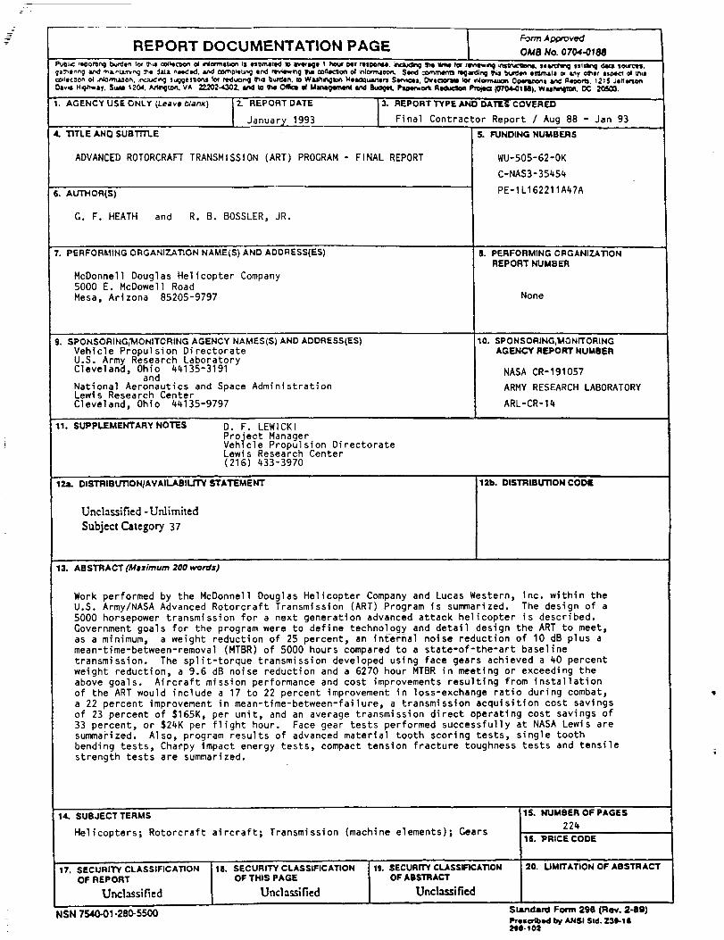
Form Approved
REPORT DOCUMENTATION PAGE [ one Noo7o4-oi.I_bh¢ reOo."_l b,urden I_ _ _lea_n _ miormst_ _s esUms_ Io _ego t _ N¢ r_tpor4e, _ _ time lot rewew_ ._=tr_ctlanL eo_'_ e=t=lr_J .4-.= sources,
Co_lec_or_ OI _oert_J_o_. _u_p_ 5u_e5_o_l foe r_uonq _r_el b_hll% _o Wi._h_'_lo_ HoI_lU, l_e_ S_'v_ls. _rt_OratO _r mlom_L_ 0_| _ Rel_. _2_5 Je_e_en
08v== M@r_,8).. Su_ _20_./Ut_r,gu_. vA 22202.4302. _ to _ Offk:= d Ma_ _ lk_ I_0¢¢ ReameD, Pmie= {07O4,OtN). Wu_w_¢mn. ¢X; 2_03.
1. AGENCY USE ONLY (Leave b/ank) 2. REPORTDATE 13. REPORTTYPEANODATE_-COVERED
January/ 1993 ! Final Contractor Report / Aug 88 - Jan 93
4. 'tITLE ANQ SUBTITLE S. FUNDING NUMBF.J_S
ADVANCED ROTORCRAFT TRANSMISSION (ART) PROGRAM - FINAL REPORT
s. AUTHOR(S)
G. F. HEATH and R.B. BOSSLER, JR.
7. PERFORMING ORGANi_,_ON NAME(S) AND ADDRESSIES)
McDonnell Douglas Helicopter Company5000 E. McDowel] Road
Mesa, Arizona 85205-9797
9. SPON$ORING_ONITORING AGENCY NAMES(S) AND ADDRESS(ES)
Vehicle Propulsion DirectorateU.S. Army Research LaboratoryCleveland, Ohio 44135-3191
and
National Aeronautics and Space AdministrationLewis Research Center
Cleveland, Ohio 44135-9797
11. SUPPLEMENTARY NO11ES D. F, LEWICKIProject Manager
Vehicle Propulsion DirectorateLewis Research Center
(216) 433-3970
12a. DISTR_UTIO_AVAILABILJTYSTATEMENT
WU-S05-62-OK
C-NAS3-35454
PE-1L162211A47A
8. PERFORMING OFIGANI7_ATION
REPORT NUMBER
None
10. SPONSORING,MONITORINGAGENCY REPORT NUMBER
NASA CR-191057
ARMY RESEARCH LABORATORY
ARL-CR-14
12b. DtSTRIBLrrlON CODE
Unclassified -Unlimited
Subject Category 37
13.,,, ,,
ABSTRACT (Maximum 200 words)
Work performed by the McDonnell Douglas Helicopter Company and Lucas Western, Inc. within the
U.S. Army/NASA Advanced Rotorcraft Transmission (ART) Program is summarized. The design of a
5000 horsepower transmission for a next generation advanced attack helicopter is described.
Government goals for the program were to define technology and detail design the ART to meet,
as a minimum, a weight reduction of 25 percent, an internal noise reduction of 10 dB plus a
mean-time-between-removal (MTBR) of 5000 hours compared to a state-of-the-art baseline
transmission. The split-torque transmission developed using face gears achieved a 40 percent
weight reduction, a 9.6 dB noise reduction and a 6270 hour MTBR in meeting or exceeding the
above goals. Aircraft mission performance and cost improvements resulting from installation
of the ART would include a 17 to 22 percent improvement in loss-exchange ratio during combat,
a 22 percent improvement in mean-time-between-failure, a transmission acquisition cost savings
of 23 percent of $165K, per unit, and an average transmission direct operating cost savings of
33 percent, or $24K per flight hour. Face gear tests performed successfully at NASA Lewis are
summarized. Also, program results of advanced material tooth scoring tests, single tooth
bending tests, Charpy impact energy tests, compact tension fracture toughness tests and tensile
strength tests are summarized.
14. SUBJECT TERMS
Helicopters; Rotorcraft aircraft; Transmission (machine elements); Gears
! 17. SECURITY CLASSIFICA'TiON i 18. SECURITY CLASSIFICATION _s.SEcu_n_'c'_ssIRC*_ONOF REPORT OF THIS PAGE OF ABSTRACT
Unclassified Unclassified Unclassified
NSN 7540-01-280-5500
15. HUMBER OF PAGES
224
16. "PRICE CODE
i 20. UMrrATION OF ABSTRACT
PreserVed by ANSI SId. Z3_-1 a:_Jg-_02