Embed Size (px)
Citation preview

V 13 no 4 bull MarApr 2010
Indirect Land Use One Consideration Too Many in Biofuel Regulation David Zilberman Gal Hochman and Deepak Rajagopal
One of the major objectives of renewable fuel policies in the United States is to introduce
alternative fuels that reduce green-
However a unique feature of biofuel regulation is that the traditional LCA is augmented to account for the indirect land-use effects (ILUEs) associated with
Allocation of agricultural commodities like corn to produce biofuels (ethanol)mdash leads to higher corn prices which may lead to expansion of corn acreage and ultimately expansion of agriculture resulting in extra greenhouse gas (GHG) emissions from land use These extra emissions are what are referred to as indirect land-use effects (ILUEs) of biofuels This paper argues against the current practice of considering ILUEs of biofuels in the current California and Federal regulations of biofuel The indirect land uses are uncertain vary over time and their current estimates diverge significantly
Also in this issue
Can Improved Market Information Benefit Both Producers and Consumers Evidence from the Hass Avocado Boardrsquos Internet Information Program Hoy F Carman Lan Li and Richard JSexton5
End of Life Vehicles and Air-Conditioning Refrigerant Can Regulation Be Cost Effective Emily Wimberger and Jeffrey Williams9
house gas (GHG) emissions relative to fossil fuels Thus the Energy Indepenshydence and Security Act of 2007 (EISA) requires that transportation fuels sold in the United States contain a minishymum volume of biofuels and requires a national renewable fuel standard (RFS) Enforced by the US Environshymental Protection Agency the RFS sets an upper bound on GHG emission per unit of various biofuels For example corn ethanol meets the RFS if (after the appropriate adjustments) it reduces the GHG emission by 20 relative to gasoline Another major regulation of biofuels is the low carbon fuel stanshydard (LCFS) which unlike the RFS concerns all fuels It was introduced by California as part of AB32 and is under consideration by other states and also the EU and China The California standard requires reduction of the average GHG emission of fuels by a certain percentshyage each year until attaining the evenshytual target of 10 reduction by 2020
The GHG emission of different fuels in these regulations is calculated using life cycle analysis (LCA) Traditionally this technique calculates all the emisshysions that are generated throughout the life of a biofuel including the emissions generated in production of fertilizers plowing of the fields harvesting proshycessing as well as burning of the fuel
the production of biofuel For example if producing biofuel from corn led to the expansion of agricultural land and conversion of rangeland or forest to agriculture this ILUE is considered as part of the LCA One possible pathway leading to land-use change is shown in figure 1 on page 2 The idea that biofuel regulations needs to take into account the ILUE was motivated by an influential paper by Searchinger et al (2008) This notion is based on the basic properties of market behavior In particular when the demand for a product like corn is expanding in our case because of the introduction of biofuels the increase in the price of the product leads to increased supply The increased supply of corn may lead to land conversion to agricultural production and this process of expanding the agricultural land base leads to release of extra GHG emissions These extra GHG emissions have to be calculated as they are the indirect land-use components of the LCA of biofuels Figure 1 provides a graphical presentashytion of the LCA and the indirect land uses of biofuels While including ILUEs in assessing the impact of biofuel seems appealing we will argue here against an indirect land use in biofuel regulations for the basic reason that its inclusion in LCAs contradicts a basic principle of regulationmdashnamely that individuals
Figure 1 One Pathway for Indirect Land Use Change
US biofuel policy increases demand for corn for ethanol
Corn prices increase and US farmers plant more corn and
reduce soybean planting
Reduction in soy exports from US and world soy prices increase
Farmers in Brazil plant more soy at the expense of pasture land for cows
Increase in beef prices
Forest cleared in Brazil for pasture land
Release of carbon stored in treessoil
are responsible only for actions that they control The indirect land uses are difficult to compute and vary over time Finally there are other indirect effects of biofuels that are not included in the LCAs of biofuel and thus the inclusion of indirect land use is inconshysistent with other regulatory criteria
Use of Indirect Land Use Contradicts the Sound Principle of Policy Design The technical difficulty in estimating indirect land use is only one reason why this concept is not appropriate to use in regulating biofuels Economists introduced the notion of an externality It occurs when the activities of one ecoshynomic agent say a farmer has an uninshytended effect on the well-being of others They distinguish between technical and pecuniary externalities Negative technishycal externalities occur when for examshyple waste materials from farms contamishynate the water of a nearby fishery In this case economic theory suggests it is socially desirable that the polluters will take into account the extra contaminashytion cost in choosing their activities
Pecuniary externalities occur when the activities of a group of economic agents affect the well-being of others through markets by changing prices When the industry is competitivemdashand for example when a group of economic agents increases their demand for a
product the price of the product increases and more of the product will be produced Other buyers of the prodshyuct will suffer from the pecuniary extershynality (the price increase) Economic theory suggests that the industry shouldnrsquot be responsible for the impact of the rising prices Moreover if the increase in production will result in more pollution namely a technical externality resulting from the pecuniary externality then economic theory sugshygests that policy intervention should be enacted to modify the polluting activishyties of the producers of the extra supply
The difference in the treatment of technical and pecuniary externalities is that producers control their production and hence their pollution But in a comshypetitive market they donrsquot control the prices This reflects a basic principle Individuals should be responsible for activities that they control and not for those that they donrsquotThis basic message of accountability suggests that producers of biofuel shouldnrsquot be held responsible for indirect land-use decisions made by others
The use of a traditional LCA for environmental regulation is justified on informational and control considershyations The production of biofuel may involve supply chains with many entishyties that are vertically linked through contractual arrangements When the final seller of biofuel say an oil
company is held accountable for the life cycle emission it may be much more effective in obtaining informashytion and affecting choices throughout the supply chain than a government entity when it attempts to regulate each entity separately Holding the final seller of a supply chain responsible for emissions and other externalities throughout the supply chain is a growshying tendency that has led to increased emphasis on traceability and resulted in regulations based on LCA in other sectors of the economy While the sellshyers of the biofuels are aware and can affect the behavior of their suppliers and other agents up the supply chain they cannot affect the choices of proshyducers in another industry (farmers in Brazil) and the indirect land use lacks one of the advantages of the use of trashyditional LCAs in regulating biofuels
Furthermore there is a related flaw in the use of indirect land use for regushylating biofuels Basic principles of public economics suggest that all emitters of GHGs in the world are held responsible for their own activities The indirect land-use approach holds farmers responshysible for possible emissions by farmers elsewhere Searchinger et alrsquos arguments imply that since the Brazilian governshyment may not fully control deforestation in the Amazon we should make sure that US biofuel producers would be held responsible for activities that will raise the price of corn and soybean and may lead agents in Brazil to deforest the Amazon and increase GHG emissions It makes more sense to strive to enact polishycies that will make Brazil or any other country responsible for the GHG emisshysions associated with land-use changes in their countries through international agreement rather than make agents in the United States or elsewhere responshysible for the lack of action in Brazil It is impractical to assume that by modifying the biofuel policies in the United States one can forever protect the tropical forests in Brazil or anywhere There is
Giannini Foundation of Agricultural Economics bull University of California 2
an old principle of policymaking that each policy tool should concentrate on controlling a policy objective When LCA regulations aimed to control the choices of biofuel suppliers to the U S market and also are designed at least implicitly to affect land-use choices of other agents they are likely to under-perform in all tasks Biofuel policies are part of a set of land-use policies that try to achieve multiple objectives including control of GHG preservation of biodishyversity provision of environmental ameshynities and production of food and fiber within a globalized economy Whenever market prices do not capture social costs or benefits specialized policies should be designed to address the technical externalities of biofuels land-use expanshysion and biodiversity preservation
The ILUEs of Biofuels Change Frequently and Are Difficult to Implement Recent attempts of computing the ILUEs of biofuels have encountered some problems First different studies derived significantly different estimates of the ILUEs For example a forthcoming study by Hertel et al (2010) estimates the magnitude of the ILUE of biofuel to be one-third of the one estimated effect by Searchinger et al (2008) This is not surprising since the computed change in land use and emission of GHGs is based on responses to commodity prices which are diverse and have varied drasshytically between countries and among crops over time Higher commodity prices may lead to increased agricultural acreage andor intensification of agriculshytural production by adoption of more efficient production technologies or increase in the use of inputs like fertilshyizers Land-use changes are more likely to contribute significantly to increased overall agricultural supply in periods of low rates of change in agricultural proshyductivity and be less important in perishyods of large gain in productivity The recent study by Alston Beddow and
Pardey (2009) suggests that the changes in agricultural productivity vary signifishycantly among regions and over time
Further changes in productivities are strongly affected by policy Zilbershyman et al (1991) suggest that banshyning the use of pesticides for example might have led to a strong increase in acreage as yield per acre would have declined A recent study by Sexton and Zilberman (2010) suggests that the adoption of genetically modishyfied (GM) corn soybeans and cotton increased yield substantially In the absence of this productivity increase acreage would have been rising They calculate that without the adoption of GM crops some prices of agricultural commodities like corn would have risen by 30 They also argue that if the practical ban of biotechnologies in European and African countries had been removed much of the increase in food prices attributed to biofuels would have been eliminated Historically agrishycultural production has grown much faster than arable land According to Federico (2009) the world agricultural production more than tripled between 1950 and 2000 while acreage in arable land and tree crops grew by less than 25 US agricultural acreage peaked around 1920 and even though producshytivity output has increased by ten- fold since then the acreage has declined
Computation of the ILUE does not end in estimating the expansion of agricultural land because of biofuel It requires quantitative understanding of the conversion of various ecosystems (forest and pasture) to agriculture and their implications on GHG There is a big difference from the GHG perspecshytive whether an increase in the acreage of corn would result in conversion of old-growth forest or wildland to farmshying Some of the increases in soybean acreage in South America in recent years were ldquovirtualrdquo increases namely farmshyers started double-cropping soybeans following wheat which might have
led to carbon sequestration and reduce GHG emissions The uncertainty about the conversion of ecosystems to farmshying is a major reason for the differences between indirect land-use estimates However the conversion processes and their GHG implication can be affected by policies and technologies Better enforcement of policies to conshytrol deforestation as well as incentives for carbon sequestration may drastishycally affect the GHG impact of agriculshytural expansion because of biofuels
Thus it would be very difficult to predict the ILUEs of specific biofushyels as they are unstablemdashaffected by changes in weather economic condishytions and knowledge They can also be influenced by policy choices for example more investment in agriculshytural research more liberal regulation of biotechnology or changes in the deforestation and land-use policies
Consistency and Incentive Considerations The introduction of indirect land use in the context of biofuel is inconsisshytent with other types of policies The introduction of biofuel has other indishyrect effects through the markets For example one can consider the indirect fuel price effects associated with bioshyfuel Recent studies suggest that the introduction of biofuel has reduced the price of fuels by 1ndash2 which results in extra driving and an increase in congesshytion and GHG emissions On the other hand by reducing the price of fuel the introduction of biofuel may make it less profitable to invest in oil produced from tar sands and to convert coal to oil This may reduce GHG emissions because conversion of tar sands for oil is highly contaminating Furthermore the increase in supply of biofuels may lead the Organization of the Petroleum Exporting Countries (OPEC) to reduce some of their production activities
And again the indirect effect through the markets also affects GHG emissions
Giannini Foundation of Agricultural Economics bull University of California 3
So if we start to consider some indirect effects on GHGs associated with biofuel we should consider them all But then where lies the end And how can we calculate them all Why should we hold producers responsible for things that they cannot control There is another source of inconsistency that one has to recognize when considering indirect land use The conservation reserve proshygram (CRP) in the United States and other reserve programs are improving environmental qualitiesmdashand providshying a significant amount of ecosystem services by diverting land from agriculshytural production and in many cases the production of corn and soybean By taking corn and soybean out of proshyduction the CRP has indirect land-use effects that may lead to expansion of production in other parts of the world with negative environmental impacts Are these ILUEs taken into account when farmersrsquo proposals for diversion of land through CRP are evaluated
Biofuels to a large extent are works in progress Our methods of crop proshyduction processing conversion and utishylization of biofuels are far from perfect We rely on first-generation biofuels that in some cases may generate more GHG emissions than they sequester However at the same time we aim to encourage technological development that will improve the GHG performance of existshying biofuels which leads to introduction of more sustainable second-generation biofuels We allocate a large amount of public research but these technologies will not be improved and introduced without major private investment The introduction of biofuel plants is subject to incentives and regulations and it is expected that the GHG performance of the new facilities will be far supeshyrior to that of the current facilities
However indirect land uses introshyduce uncertainty because the perforshymance standards under which new facilities will be judged will not be conshytrolled by their own design but by the
performance of other actors that they cannot control Increased uncertainty is a disincentive for investment and indishyrect land use may inadvertently lead to underinvestment in second-generation biofuels or improvement in current bioshyfuels From an investorrsquos perspective it may be more sound to have policies that become stricter over time than policies that are inherently uncertain Thus the indirect land use that is part of the attempt to reduce GHG effects of biofuels may have the opposite effect by providing this incentive to invest in new and cleaner biofuel technologies
Conclusions The indirect land-use concept reflects good intentions but has many practishycal and logical flaws When individushyals are regulated based on the indirect land use of their biofuels they become responsible for actions that they do not control Current policies are inconsisshytent since they consider one type of indirect effect of biofuels while ignorshying others The ILUEs of biofuels are unstable may vary significantly over time and with policy choices and are difficult to implement Their inclushysion in biofuel regulations introduces unnecessary uncertainty about future regulations which hampers investment choices Thus the use of indirect land use in the current regulations of the GHG emissions of biofuels represents a well-intentioned unilateral effort to control one aspect of climate change but it may be counterproductive
Removal of ILUEs from LCAs will present an improvement of biofuel regulations But stand alone biofuel or renewable fuel policies not integrated with controls of other GHG emissions are far from ideal Climate change is a global problem requiring consistent policy responses throughout the world Efficient control of climate change requires equilibrating the implied prices of GHG emissions across activities Designing procedures and mechanisms
to further improve biofuel utilization and prices is an important subject for future research and policymaking
David Zilberman is a professor and Gal Hochman is an assistant researcher both in the Department of Agricultural and Resource Economics at UC Berkeley They can be contacted by e-mail at zilber11berkeleyedu and galhberkeleyedu respectively Deepak Rajagopal is a postdoctoral scholar at the Energy Biosciences Institute at UC Berkeley His e-mail is deepakberkeleyedu
For further information the authors recommend
Alston Julian M Jason M Beddow and Philip G Pardey 2009 Mendel versus Malthus Research Productivshyity and Food Prices in the Long Run Staff Papers 53400 University of Minnesota Department of Applied Economics
Federico Giovanni 2009 Feeding the World An Economic History of Agrishyculture 1800-2000 (Princeton New Jersey Princeton University Press)
Hertel TW AA Golub AD Jones M OrsquoHare RJ Plevin DM Kamshymen 2010 Global Land Use and Greenhouse Gas Emissions Impacts of US Maize Ethanol Estimating Marshyket-Mediated Responses Forthcoming in Bioscience
Searchinger Timothy Ralph Heimshylich R A Houghton Fengxia Dong Amani Elobeid Jacinto Fabiosa Simla Tokgoz Dermot Hayes and Tun-Hsiang Yu (29 February 2008) Use of US Croplands for Biofuels Inshycreases Greenhouse Gases Through Emissions from Land-Use Change Science Vol 319 no 5867 pp 1238 ndash 1240
Sexton Steve and David Zilberman The Economics of Agricultural Bioshytechnology Adoption Implications for Biofuel Sustainability Paper preshysented in the Agricultural Economic Conference of the NBER Boston MA March 3 2010
Zilberman David Andrew Schmitz Gary Casterline Erik Lichtenberg and Jerome B Siebert (2 August 1991) The Economics of Pesticide Use and Regulation Science Vol 253 No 5019 pp 518-522
Giannini Foundation of Agricultural Economics bull University of California 4
Can Improved Market Information Benefit Both Producers and Consumers Evidence from the Hass Avocado Boardrsquos Internet Information Program Hoy F Carman Lan Li and Richard J Sexton
We estimate benefits to consumers and avocado producers of the Hass Avocado Boardrsquos market-information program Evidence suggests that the program stabilized shipping point prices reduced the farm-retail marketing margin and conferred benefits to both consumers and producers
Retail margins for avocados will tend to increase with larger and more frequent price changes and decrease with smaller and less frequent price changes
The Hass Avocado Board (HAB) is a US government-sponsored marketing program funded by a
producer assessment of 25 cents per pound on all domestically produced and imported Hass avocados sold in the US market While the HAB allocates the majority of its funds to advertisshying and promotion programs it also conducts an innovative Internet inforshymation program through its Network Marketing Center Growers packers shippers and wholesalers in the United States Chile Mexico Dominican Republic and New Zealand as well as US retailers have access to the HAB web site where they share marketing information including harvest shipshyment and price data The ldquoorderly marshyketingrdquo goal of information exchange is to smooth shipments to major US markets prevent seasonal surplus and shortage situations and promote stable shipping-point and retail prices
Government market-information programs have been justified based on their contributions to improved market outcomes especially when there are significant differences in market power between buyers and sellshyers However the availability of timely information has decreased over time as marketing channels for agricultural products have become more direct replacing central wholesale markets Government budget issues and a lack of reliable estimates of the benefits of market-information programs have also contributed to their elimination Now however advances in communications and information technology provide a framework for innovative and effecshytive market-information programs
The HAB information program is an example of one such program In this article we estimate the impact of the HAB program on shipping-point price variability and avocado marketshying margins Costs and benefits of the program to both consumers and Hass avocado producers are estimated
Analytical Framework US supermarkets have market power that is evident in their pricing pracshytices An analysis of price transmission for avocados found that retail prices for avocados respond more fully to shipping-point price increases than to shipping-point price decreases Speshycifically Li estimated that on average 76 of an increase in shipping-point price is passed on to retail compared to only 29 of a decrease in the shipshyping-point price As a result retail marshygins for avocados will tend to increase with larger and more frequent price changes and decrease with smaller and less frequent price changes
Price instability thus promotes higher retailer margins and increased price stability will tend to decrease annual average retailer margins Inforshymation programs that smooth the flow-to-market of avocados stabilize prices and reduce marketing margins can benefit both producers and consumers through higher average shipping-point prices and lower average retail prices
To estimate the impact of price varishyability on avocado marketing margins we proceeded as follows (1) the varishyance and standard deviation of weekly shipping-point prices before and after initiation of the HAB information proshygram were calculated and compared
Giannini Foundation of Agricultural Economics bull University of California 5
2000
1998
2006
2004
2002
1964
1962
1984
1982
1980
1978
1976
1972
1970
1968
1966
1992
1990
1988
1986
1996
1994
1974
Figure 1 Inflation-adjusted Annual Average California Shipping-point Price for Avocados 1962ndash2007
120
100
80
60
40
20
0
Cen
ts
(2) using Lirsquos estimates of marketing margin adjustments to shipping-point price changes the estimated average annual change in the standard deviashytion of weekly prices after program initiation was used to simulate weekly changes in estimated marketing marshygins and (3) using estimated price elasticities of demand the changes in estimated marketing margins were alloshycated between the retail and shipping-point levels in the marketing channel
Results
Year
The variance and standard deviation of weekly California shipping-point avocado prices were calculated for each year of the ten-year period 1998 through 2007 This period was selected to include the five years before (1998 through 2002) and the five years after (2003 through 2007) initiation of the HAB information program
The real (inflation-adjusted) annual average California shipping-point price for avocados is shown in figure 1 for 1962ndash2007 Annual average prices
mask considerable intrayear variabilshyity in prices The standard deviation of weekly average prices for the most recent five years 2003ndash07 averaged 02045 a decrease from the weekly average standard deviation of 02843 for the prior five years Thus the average annual standard deviation of weekly prices decreased 28 from the five years immediately before initiashytion of the HAB information program to the first five years after initiation of the information program At the same time the annual average stanshydard deviation of California weekly shipments increased from the first five years (1998 through 2002) to the most recent five years (2003 through 2007) while the standard deviation of total weekly shipments (Califorshynia plus all imports) decreased
This indicates that coordination of imports with California shipments has smoothed total weekly avocado shipments and prices during the marshyketing year While growing imports had the potential to introduce addishytional quantity and price variability into the US market the opposite has occurred Imports have been timed to maintain a rather steady flow of avoshycados to retail markets which tends to stabilize prices at both the shipping-point and retail levels A portion of the smoothing of quantity and prices
Information for the analysis is from the Avocado Marketing Research and Information Center (AMRIC) system AMRIC created by California law in 1985 provides the California avocado industry with daily inventory and shipshyment information to guide harvest market strategies AMRIC has develshyoped a strong database on avocado prices and inventories by variety and size as well as shipments by major market destination variety and size Avocado Price Variability The HAB information program was initiated during the 2002ndash2003 marketing year
Table 1 Estimated Total Annual Changes in Gross Margins for Hass Avocados Average Shipments Standard Deviation of Price and Average Price 2003-2007
Year
Item estimate 2003 2004 2005 2006 2007
Margin change ($) 6533780 2889059 8133135 4033952 10070172
Ave weekly shipments (lbs)
8512807 11771751 12484837 15194896 13361154
Std deviation of price ($lb)
0271 0128 0216 0058 0263
Average weighted shipping point price ($lb)
1136 1018 0955 0761 0993
Source Calculated from weekly price and shipment data provided by the California Avocado Commission Avocado Marketing Research and Information Center (AMRIC)
Giannini Foundation of Agricultural Economics bull University of California 6
as imports increased significantly can and should be attributed to the active HAB information programs Marketing Margin Adjustments The results from Lirsquos research on price transmission in the marketing chanshynel were used to estimate weekly changes in gross marketing margins between the shipping-point price and the retail price of avocados We assumed that 76 of the increase in shipping-point prices was passed on in the form of higher retail prices and 29 of a decrease in shipping-point prices was passed on to consumers in the form of lower retail prices The changes in estimated gross marketing margins from week to week are based on total weekly shipments the change in average weighted shipping-point price per pound for all Hass avocados and Lirsquos estimated adjustment ratios
Annual estimated gross changes in marketing margins based on each marketing yearrsquos weekly total Hass avoshycado shipments and weighted weekly average Hass avocado shipping-point prices are shown in table 1 The actual annual standard deviations of weekly Hass avocado shipping-point prices both decrease and increase from year to year ranging from a high of 0271 in 2003 the first year of the informashytion program to a low of 0058 in 2006 a year of record weekly shipments due to a very large California crop Estimated total changes in marketing margins associated with shipping-point price changes vary from $2889059 in 2004 to just over $10 million in 2007 Note that the total changes in marketing margins are positively related to average weekly shipments and the standard deviation of weekly prices during the marketing year Estimated Information Program Benefits The simulated changes in marketing margins due to actual weekshyto-week changes in shipping-point prices are shown in table 1 To estishymate the benefits of the information
Year Grand
Total ($) Cost Category 2003 2004 2005 2006 2007
Table 2 Annual and Total Costs of HAB Information Programs by Cost Category 2003ndash2007
Information ($) 28619 219553 71104 123434 94226 536936
Analysis ($) 0 44843 168976 197375 120281 531475
Interaction ($) 286560 658956 378566 404241 397592 2125915
Network Marketing Center ($) 0 166876 66163 179052 118423 530514
Total Information($) 340179 1090228 684809 904102 730522 3749840
Source HAB Annual Reports 2003ndash2007
program we must estimate what the price variability would have been without the HAB information proshygram Our approach is to compare the variability of prices immediately before initiation of the information program with variability of prices after beginning the information program A limitation of this approach is that the entire change in price variability is attributed to the information proshygram even if there were other factors contributing to more stable prices
As noted the standard deviation of annual California Hass avocado prices decreased from an annual avershyage of 02843 during the five-year period 1998ndash2002 to an annual avershyage of 02045 from 2003ndash2007 This decrease of 28 in price variability is used as the maximum reduction in price variability due to the HAB inforshymation program The estimated total five-year increase in avocado marketing margins due to price variability from table 1 is $31661000 Thus a reducshytion of 28 in margins would have been worth a five-year (undiscounted) total of $123 million This savings is reflected in both lower retail prices paid by consumers and higher prices to growers at the shipping point HAB Information Program Costs The annual costs of HAB information
programs are listed by category in each HAB annual report and are sumshymarized in table 2 Annual expendishytures for the information programs ranged from $340179 to $1090228 over the five years with an average annual cost of just under $750000 Total five-year costs for the categoshyries of information analysis and the Network Marketing Center were in a rather tight range of $530514 to $536936 Almost 57 of total costs for the first five years ($2125915) were in the interaction category Allocation of Net Benefits The divishysion of the total benefit as well as the assessment cost to fund the informashytion program between consumers and producers depends upon the value of consumersrsquo price elasticity of demand ED relative to producersrsquo price elasticity of supply ES of avoshycados to the US market The share of a change in margin going to conshysumers in terms of lower price is
E∆P = S
ESndash ED
Carman Li and Sexton (2010) estimated demand relationships for avocados using various combinations of functional forms and variables Estimates of the relationship between per capita quantity and real price were
Giannini Foundation of Agricultural Economics bull University of California 7
very stable regardless of the variables included Using the estimated price coefficients we evaluated ED at the average of price and quantity for the past ten years Regardless of the speshycific model estimated we obtained a value of EDasymp-025 during this ten-year period meaning that a 4 increase in price would be associated with about a 1 decrease in consumption
There are no recent studies of the price elasticity of supply for avocados Supply functions are difshyficult to estimate empirically and the elasticity of supply varies by the length of run (time frame) under considerationmdasheg supply becomes more elastic (responsive to price) in the long run as productive inputs become variable to producers
Supply analysis is particularly difshyficult for perennial crops because the analyst must normally specify a dynamic model containing equations for plantings removals bearing acreage as a function of plantings and removshyals and yield An alternative approach to studying the supply relationship is to estimate a range of plausible values for elasticity of supply If conclusions are robust across the range of supply elasticity values chosen there is little need to worry about choosing among the plausible alternative values
In considering a range of plausible values for elasticity of supply note that short-run supply of a perennial crop is highly inelastic because it is the product of bearing acreage and yield neither of which is likely to be influenced much by current price Thus the supply of avocados from California is likely to be highly inelastic The supply of imports to the United States emanating from Chile and Mexico however is apt to be more elastic because the total supply in each country can be allocated to domestic consumption or to various export markets Thus an increase in price in the United States due to facshytors such as successful promotions is
likely to cause Chilean and Mexican shippers to increase supply into the United States Based on these considshyerations we specified three alternashytive values for ES 05 10 and 20
Using ED = -025 and values of ES
ranging from 05 to 10 to 20 we calshyculated the estimated consumer and producer shares of costs and benefits from the information program Estishymated consumer shares ranged from 67ndash89 with producer shares rangshying from 33ndash11 depending upon the value assumed for ES Assuming that the entire margin reduction can be attributed to the HAB information program the total net benefit is $123 million gross benefit minus $375 million program cost or $855 milshylion net benefit Producersrsquo share of this net benefit is then in the range of $094ndash$282 million dollars with the remainder of the net benefit going to US avocado consumers
Concluding Comments Publicly available market information has costs and benefits but the costs of obtaining and disseminating informashytion are typically much easier to estishymate than the benefits or returns from having the information available to market participants The present study attempts to measure the value of an information program designed to foster orderly marketing in the US avocado market with the value of information stemming from reduced price varishyability leading to reduced marketing margins The HAB reported five-year information program expenditures of $375 million Based on a 28 reducshytion in price variability we estimated a five-year reduction in avocado marketshying margins of $123 million with net benefits totaling $855 million With an inelastic demand at recent prices and quantities the majority of estimated benefits flow to consumers although producers still receive an attractive return for their share of expenditures
Public market-information proshygrams for agricultural commodities have been under pressure for several decades as a result of changing chanshynels of distribution and decreased government funding Terminal market price and arrival data have decreased as these markets have been by-passed by the movement to direct purchase programs by large-scale food retailshyers and market reports have been reduced and suspended in response to government budget reductions
In light of the significant consumer benefits estimated for the HAB informashytion program we believe that new and innovative market-information proshygrams based on advanced information technology and rapidly evolving inforshymation delivery systems should be serishyously considered for implementation
Hoy F Carman is a professor emeritus and Richard J Sexton is a professor both in the Department of Agricultural and Resource Economics at UC Davis They can be contacted by e-mail at carmanprimalucdavisedu and richprimal ucdavisedu respectively Lan Li a research associate for the National Institute for Commodity Promotion Research at Cornell University can be reached by e-mail at ll469cornelledu
For further information the authors recommend
Carman Hoy F Lan Li and Richard J Sexton ldquoAn Economic Evaluation of the Hass Avocado Promotion Orshyderrsquos First Five Yearsrdquo Giannini Foundation Research Report 351 httpgianniniucopeduresearchreshyportshtm
Li Lan ldquoRetailer Pricing Behavior for a Fresh Produce Commodity The Case of Avocadosrdquo PhD Dissertashytion University of California Davis 2007
Giannini Foundation of Agricultural Economics bull University of California 8
End of Life Vehicles and Air-Conditioning Refrigerant Can Regulation Be Cost Effective Emily Wimberger and Jeffrey Williams
Vehicles that are no longer driven contribute to air pollution HFC-134a is a common refrigerant in vehicle air-conditioning systems and a greenhouse gas Increased regulation pertaining to the removal of HFC-134a from End-of-Life Vehicles has been proposed as a means to reduce air pollution We estimate the amount of HFC-134a that remains in vehicles that are no longer driven in California and find that increased regulation is not warranted
HFC-134a the refrigerant used in the air-conditioning sysshytems of vehicles beginning
with the 1995 model year is a toxic greenhouse gas When released into the atmosphere HFC-134a reacts with sunlight and creates ground level ozone that is detrimental to the health of humans and ecosystems As vehicles are driven small amounts of the refrigershyant leak into the atmosphere When a vehicle reaches the end of its drivable life an unknown quantity of HFCshy134a remains in its air-conditioning system possibly to leak into the atmoshysphere possibly to be recovered
Vehicles that have reached the end of their drivable lives are commonly known as End-of-Life Vehicles or ELVs ELVs have been issued either a junk title or salvage certificate by the Department of Motor Vehicles (DMV) and cannot legally be driven ELVs are often sold to dismantlers or junkyards and used for parts or metal recycling
The removal and recovery of HFCshy134a from these End-of-Life Vehicles is regulated under sections 608 and 609 of the Clean Air Act which prohibits the venting of vehicle refrigerant into the atmosphere Section 608 and section 609 of the Clean Air Act require vehicle dismantlers to remove and recycle any vehicle refrigerant contained within End-of-Life Vehicles These regulashytions however are rarely enforced
The California Air Resources Board (CARB) has identified improving the recovery rate of HFC-134a from End-of-Life Vehicles as part of its greenhouse gas reduction strategy However little is known about the quantity of HFC-134a remaining in End-of-Life Vehicles found in licensed junkyards and dismantling yards Nor is much known about the model years common in junkyards and hence about the percentage of ELVs that contain this specific refrigerant
This report presents the prelimishynary results from an analysis for CARB that estimates the portion of the ELV population containing HFC-134a and that quantifies the amount of HFCshy134a remaining in these vehicles When combined these two estimates help determine whether increased enforcement of sections 608 and 609 of the Clean Air Act is warranted
Vehicle Sampling To quantify the amount of HFC-134a remaining in End-of-Life Vehicles refrigshyerant samples were taken from 2002 vehicles on dismantler lots throughout California in two rounds of sampling An initial sample of 160 vehicles was conducted at one location in Antelope California in January 2009 later 1842 vehicles were sampled at 29 dismantler locations throughout the state The 30 participating vehicle dismantlers were
all licensed by the State of California and were members of the State of Calishyfornia Auto Dismantlers Association
The sampling was conducted by technicians certified in refrigerant handling and safety procedures from January through August 2009 The technicians entered dismantler lots and identified vehicles with enough spatial clearance to allow for sampling and refrigerant collection In order to be sampled a vehicle was required to have an operational front hood and a visible Vehicle Identification Number (VIN)
This sampling was not random as the technician had to get permisshysion from the dismantler owner before sampling and was often told which vehicles were ldquooff-limitsrdquo At some dismantler lots this restricted access meant only a handful of vehicles could be sampled Once a vehiclersquos refrigershyant was sampled the refrigerant was returned to the vehicle and the vehicle was marked for refrigerant collection As the amount of refrigerant was sampled the technician recorded vehicle-specific information including refrigerant capacshyity vehicle make vehicle model year license plate information mileage vehicle color and the overall condition of the vehicle At the end of each day of sampling the refrigerant was collected from each sampled vehicle and was reclaimed by a licensed disposal service
Sampled vehicles ranged in model year from 1970 to 2009 with a mean of 1997 and a standard deviashytion of three years There were 1536 vehicles 77 of the sample that were 1995 and newer model-year vehicles Across this sample of 2002 vehicles 1966 vehicles had air-conditioning systems utilizing HFC-134a Identifyshying the specific refrigerant used in a vehiclersquos air-conditioning system prior
Giannini Foundation of Agricultural Economics bull University of California 9
Figure 1 Model Year and Percentage of HFC-134a Recovered from Sampled End of Life Vehicles
300
250
200
150
100
50
0 1970 1975 1980 1985 1990 1995 2000 2005 2010
Year
to sampling was nearly impossible and lot were not significant in determinshy
36 vehicles containing the precursor ing the amount of HFC-134a remain-
to HFC-134a R-12 were sampled ing in the air-conditioning system
Across all sampled vehicles con- Figure 1 presents the percentage of
taining HFC-134a an average of 27 recovered HFC-134a for each sampled
of vehicle-specific refrigerant capac- End-of-Life Vehicle with the solid line
ity remained in the air-conditioning representing the average Seventeen
system However the amount of HFC- of these End-of-Life Vehicle had over
134a remaining in the air-conditioning 100 of refrigerant capacity at the time
systems of sampled vehicles varied of sampling These abnormally large
widely No HFC-134a remained in values could be the result of sampling
the air-conditioning systems of 781 errors or could be caused by incorshy
sampled vehicles The other 1185 rectly charged vehicle air-conditioning
sampled vehicles containing HFC- systems during the vehiclersquos lifetime
134a contained an average of 45 of California End-of-Life vehicle-specific refrigerant capacity Vehicle PopulationThere was also very little correlation
between the percentage of HFC-134a The California Department of Motor remaining in sampled vehicles and any Vehicles (CA DMV) does not compile geographic dismantler or vehicle-spe- statistics pertaining to junk titles and cific characteristics Across the sample salvage certificates In fact the CA DMV of vehicles containing HFC-134a the purges vehicles from their main database percentage of refrigerant was correlated if they have a long lapse in registration with model year and whether the vehicle activity whether a vehicle has been had a license plate at the time of sam- junked or moved out of state As no stashypling Vehicles with license plates tended tistics were directly available regarding to have a higher percentage of refrigerant the End-of-Life Vehicle population we remaining holding all other variables had to reconstruct what had happened constant As the model year of a vehicle to vehicles and obtain information about increased or the vehicle decreased ELVs using a two-step process We first in age the percentage of refrigerant looked at annual CA DMV registration remaining tended to increase holding records from 2000 through 2008 and all other variables constant Surpris- identified the cross section of vehicles ingly vehicle mileage collision status with a registration status that had and a proxy for the number of days lapsed from one year to the next From the vehicle had been on the dismantler 2000 through 2008 nearly 40 million
Perc
enta
ge R
ecov
ered
vehicles had a change in registration status These vehicles represented the potential population of ELVs and their unique Vehicle Identification Numbers (VINs) were submitted to CA DMV to obtain their full registration histories from some supplemental databases
Among these 40 million VINs 3190040 vehicles were issued a junk title or salvage certificate from January 1 2005 through December 31 2007 These vehicles constitute our End-of-Life Vehicle population Some vehicles may be missing yet these represent the most recent and most reliable estimate of all vehicles junked within California over a three-year period
Among these 3190040 ELVs the model year was normally distributed with a mean of 1991 and a standard deviation of seven years Of the ELVs from 2005 through 2007 32 were 1995 and newer model years These statistics are substantially different from the model-year distribution of the vehicles sampled for their refrigshyerant The population of End-of-Life Vehicles is much older than the sampled vehicles and a much smaller percentshyage would have contained HFC-134a
Of course the percentage of End-of-Life Vehicles that are 1995 and newer model years increases each year as seen in Table 1 On average the percentshyage of 1995 and newer ELVs reported to the CA DMV has increased 025 a month or 3 a year Extrapolating ahead the amount of HFC-134a in ELVs and the potential for significant
Table 1 Portion of End of Life Vehicle Population Containing HFC-134a
1995 and Newer Date Model Year ELVs
January 2000 9
January 2005 24
January 2006 27
January 2007 29
January 2015 (Projected) 50
January 2023 (Projected) 99
Giannini Foundation of Agricultural Economics bull University of California 10
environmental damage will not be fully realized for many years to come
We also analyzed End-of-Life Vehicles by the vehicle age at the time it was issued a junk title or salvage cershytificate Each year from 2000 through 2007 the average age of an ELV has increased on average by two months In 2000 the average age of an ELV was 14 years 9 months by 2007 the avershyage End-of-Life Vehicle was 16 years 2 months old Thus while the percentshyage of 1995 and newer model-year vehicles is increasing the population of ELVs is also increasing in age
The ELV population from 2005 through 2007 was owned by 1629 vehishycle dismantlers within California as well as 210 non-dismantling and out-of-state businesses Table 2 outlines the breakshydown of End-of-Life Vehicle ownership
CARB and US EPA only have jurisdiction over licensed vehicle dismantlers in California Thus the benefits of increased enforcement of section 608 of the Clean Air Act pershytaining to the removal and disposal of HFC-134a will be limited to only those ELVs that are on licensed vehicle dismantler lots in Californiamdash79 of all ELVs from 2005 through 2007
Results and Conclusions In determining the benefit of efforts by CARB to support US EPArsquos regulations governing the removal of HFC-134a we estimated the average amount of HFC-134a remaining in End-of-Life Vehicles and extrapolated this findshying to all vehicles in the ELV fleet that contained HFC-134a We have focused on the time frame 2005 through 2007 as this period represents the most recent and most accurate information available from CA DMV From 2005 through 2007 there were 1020938 1995 and newer model-year ELVsmdash an average of 340313 a year Assumshying the sample average of 220 grams of recovered refrigerant an average of 74869 kg of HFC-134a was left in the
Category Percentage of ELVs Owned
Table 2 Last Known Owner of End of Life Vehicles by Category
Number of Businesses
Licensed California Dismantler 79
Non-Licensed California Dismantler 1
Out-of-State and Non-Dismantler Businesses 15
Private Individual and Unidentified Entities 5
1518
111
73
137
air-conditioning systems of vehicles on California dismantler lots each year
Assuming the conditions from 2005 through 2007 persist the porshytion of ELVs containing HFC-134a will continue to increase by approxishymately 3 a year and the average age of End-of-Life Vehicles will increase approximately two months a year This translates to an increase of 54203 ELVs containing HFC-134a from 2008 through 2012 Assuming the mean HFC-134a recovered from each ELV remains at 220 grams through 2012 we project that an additional 10949 kg of HFC-134a will remain in the ELV population Thus while approximately 74869 kg of HFC-134a remained in vehicles on California dismantler lots each year from 2005 through 2007 by 2012 it will increase to 86793 kg
There are large variations in the amount of HFC-134a remaining in ELVs as well as the portion of the fleet that contains the refrigerant This variation is due to large differences among vehicles in the rate of dissipation of HFC-134a as well as the ever-changing profile of the ELV population The potential benshyefit to any actions by the California Air Resources Board to enforce sections 608 and 609 of the Clean Air Act will be affected by this variance In addition any benefit of increased enforcement will be restricted to the 79 of ELVs that were on licensed dismantler lots in California Thus while 74869 kg of HFC-134a remained on vehicle dismantler lots in California from 2005 through 2007 only 59146 kg was on licensed vehicle disshymantler lots The presence of unlicensed dismantlers reduces the potential benshyefit of any efforts by the California Air
Resources Board now and into the future to enforce regulations on HFC-134a
Given the wide range of refrigerant that was recovered from sampled vehishycles along with the inability to identify the specific refrigerant within a vehiclersquos air-conditioning system enforcing the removal of HFC-134a from End-of-Life Vehicles would be extremely difficult and expensive From 2005 through 2007 only one out of every three Endshyof-Life Vehicles contained HFC-134a and 40 of those vehicles had no HFCshy134a remaining in their air-conditioning systems Only 220 grams of HFC-134a 26 of capacity was recovered from sampled End-of-Life Vehicles which suggests that increased regulation would most likely not be cost effective
Further research into the leakage of HFC-134a during a vehiclersquos drivshyable life or increased enforcement of vehicle dismantling licensing may presshyent better options for decreasing the release of such a harmful greenhouse gas into the atmosphere While sections 608 and 609 of the Clean Air Act were necessary in order to present guidelines to vehicle dismantlers regarding the handling of HFC-134a their enforceshyment may be counterproductive at this time The complexity of the vehicle lifecycle and the factors influencing the dissipation of HFC-134a into the atmosphere may be too complex for the regulations as they currently exist
Emily Wimberger is a PhD candidate and Jeffrey Williams is a professor both in the Department of Agricultural and Resource Economics at UC Davis They can be reached by e-mail at emilyprimalucdavisedu and williams primalucdavisedu respectively
Giannini Foundation of Agricultural Economics bull University of California 11
Department of Agricultural and Resource Economics UC Davis One Shields Avenue Davis CA 95616 GPBS
Agricultural and Resource Economics
UPDATE
Co-Editors
Steve Blank David Roland-Holst
Richard Sexton David Zilberman
Managing Editor and Desktop Publisher
Julie McNamara
Published by the Giannini Foundation of Agricultural Economics
httpgianniniucopedu
ARE Update is published six times per year by the Giannini Foundation of Agricultural Economics University of California
Domestic subscriptions are available free of charge to interested parties To subscribe to ARE Update by mail contact
Julie McNamara Outreach Coordinator Department of Agricultural and Resource Economics University of California One Shields Avenue Davis CA 95616 E-mail julieprimalucdavisedu Phone 530-752-5346
To receive notification when new issues of the ARE Update are available online submit an e-mail request to join our listserv to julieprimalucdavisedu
Articles published herein may be reprinted in their entirety with the authorrsquos or editorsrsquo permission Please credit the Giannini Foundation of Agricultural Economics University of California
ARE Update is available online at wwwageconucdaviseduextensionupdate
The University of California is an Equal OpportunityAffirmative Action employer
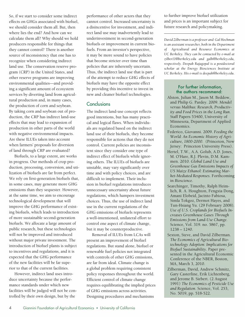
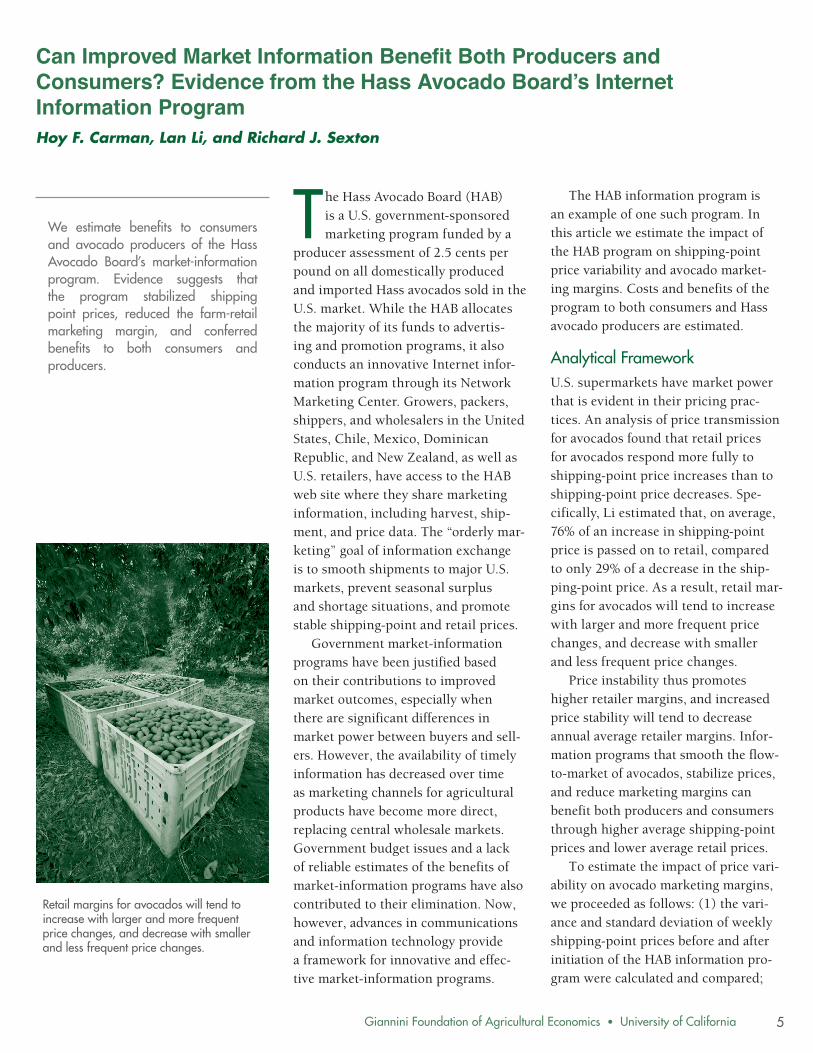
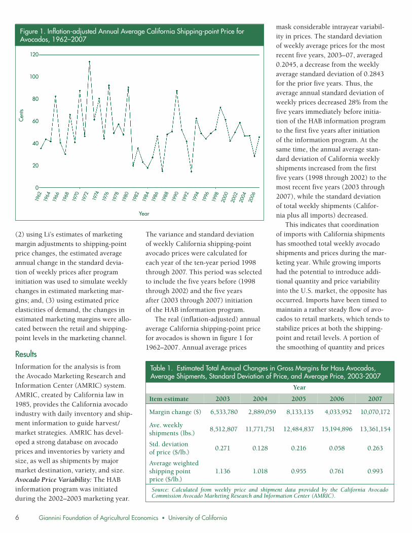
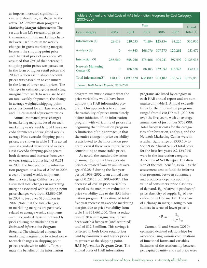
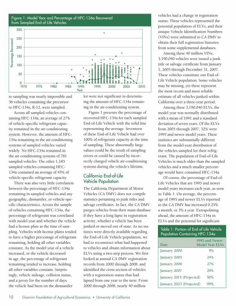
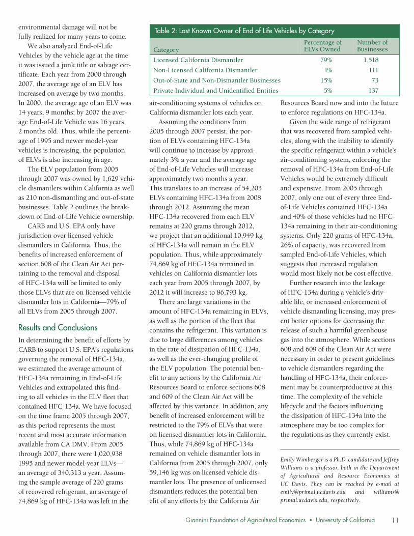