v. 10 - Aquaveogmstutorials-10.0.aquaveo.com/MODFLOW-ETSPackage.pdf · Notice that the tutorial left NETSEG at 1. This means there is one curve segment, which This means there is

Page 1 of 20 © Aquaveo 2015

GMS 10.0 Tutorial

MODFLOW – ETS Package The MODFLOW Evapotranspiration Segments (ETS) package interface in GMS

Objectives Learn how to use the MODFLOW Evapotranspiration Segments (ETS) package interface in GMS and

compare it to the regular MODFLOW Evapotranspiration (EVT) package.

Prerequisite Tutorials MODFLOW – Conceptual

Model Approach I

Required Components Map Module

Grid Module

MODFLOW

Time 40-60 minutes

v. 10.0


1 Introduction ......................................................................................................................... 2 1.1 Outline .......................................................................................................................... 3

2 Description of Problem ....................................................................................................... 4 3 Getting Started .................................................................................................................... 4 4 Open the existing model ...................................................................................................... 4 5 Save the model with a new name ....................................................................................... 5 6 Add ET via the EVT package ............................................................................................. 5

6.1 Turn on the EVT package ............................................................................................ 5 6.2 Specify ET .................................................................................................................... 5

7 Save and run MODFLOW ................................................................................................. 6 8 Examine the flow budget .................................................................................................... 7 9 Save the model with a new name ....................................................................................... 7 10 Add ET via the ETS package ............................................................................................. 7

10.1 Turn off the EVT package and turn on the ETS package ............................................. 7 10.2 Specify ET .................................................................................................................... 8 10.3 Switch LMT package to extended header .................................................................... 8

11 Save and run MODFLOW ................................................................................................. 8 12 Examine the flow budget .................................................................................................... 9 13 Saving the model with a new name .................................................................................... 9 14 Adding ETS curve segments ............................................................................................... 9

14.1 Change NETSEG ....................................................................................................... 11 14.2 Define the PXDP data ................................................................................................ 11 14.3 Define the PETM data ................................................................................................ 12

15 Saving and running MODFLOW .................................................................................... 13 16 Saving the model with a new name .................................................................................. 13 17 Building a Conceptual Model ........................................................................................... 13

17.1 Create the Conceptual Model ..................................................................................... 13 17.2 Create a Coverage ...................................................................................................... 13 17.3 Create the polygon ..................................................................................................... 14 17.4 Set the Polygon Properties ......................................................................................... 15

18 Map MODFLOW .......................................................................................................... 16 19 Examine the ETS Package ................................................................................................ 16 20 Saving and running MODFLOW .................................................................................... 16 21 Saving the model with a new name .................................................................................. 17 22 Parameters ......................................................................................................................... 17

22.1 Parameterizing the Model .......................................................................................... 17 23 Saving and running MODFLOW .................................................................................... 19 24 Conclusion.......................................................................................................................... 20 25 Notes ....................................................................................... Error! Bookmark not defined.

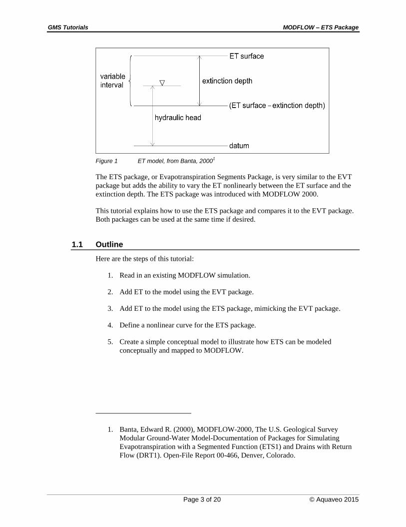
1 Introduction

Evapotranspiration is the moving of water from the ground surface to the atmosphere

through evaporation and transpiration. MODFLOW has two standard packages that are

used to model evapotranspiration: the EVT package and the ETS package. GMS has long

supported the EVT package, and, starting at version 7.0, GMS supports the ETS package.

The EVT package has existed at least since MODFLOW 88. It requires three parameters

to determine evapotranspiration: the evapotranspiration (ET) surface elevation, the

maximum ET rate, and the extinction depth. When the head in a cell is at or above the

ET surface, ET occurs at the maximum ET rate. When the head is below the extinction

depth, ET is zero. In between these two points, the ET varies linearly.

GMS Tutorials MODFLOW – ETS Package


Figure 1 ET model, from Banta, 20001

The ETS package, or Evapotranspiration Segments Package, is very similar to the EVT

package but adds the ability to vary the ET nonlinearly between the ET surface and the

extinction depth. The ETS package was introduced with MODFLOW 2000.

This tutorial explains how to use the ETS package and compares it to the EVT package.

Both packages can be used at the same time if desired.

1.1 Outline

Here are the steps of this tutorial:

1. Read in an existing MODFLOW simulation.

2. Add ET to the model using the EVT package.

3. Add ET to the model using the ETS package, mimicking the EVT package.

4. Define a nonlinear curve for the ETS package.

5. Create a simple conceptual model to illustrate how ETS can be modeled

conceptually and mapped to MODFLOW.

1. Banta, Edward R. (2000), MODFLOW-2000, The U.S. Geological Survey

Modular Ground-Water Model-Documentation of Packages for Simulating

Evapotranspiration with a Segmented Function (ETS1) and Drains with Return

Flow (DRT1). Open-File Report 00-466, Denver, Colorado.



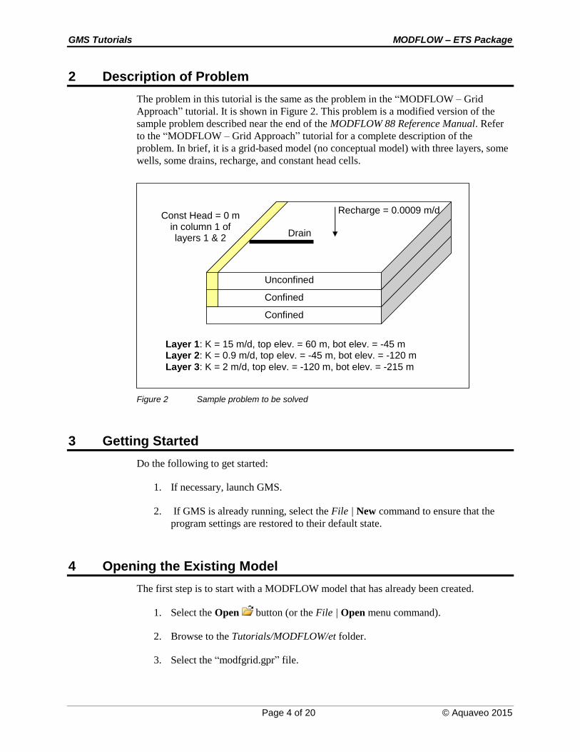
2 Description of Problem

The problem in this tutorial is the same as the problem in the “MODFLOW – Grid

Approach” tutorial. It is shown in Figure 2. This problem is a modified version of the

sample problem described near the end of the MODFLOW 88 Reference Manual. Refer

to the “MODFLOW – Grid Approach” tutorial for a complete description of the

problem. In brief, it is a grid-based model (no conceptual model) with three layers, some

wells, some drains, recharge, and constant head cells.

Unconfined

Confined

Confined

Const Head = 0 m in column 1 of layers 1 & 2

Drain

Layer 1: K = 15 m/d, top elev. = 60 m, bot elev. = -45 m Layer 2: K = 0.9 m/d, top elev. = -45 m, bot elev. = -120 m

Layer 3: K = 2 m/d, top elev. = -120 m, bot elev. = -215 m

Recharge = 0.0009 m/d

Figure 2 Sample problem to be solved

3 Getting Started

Do the following to get started:

1. If necessary, launch GMS.

2. If GMS is already running, select the File | New command to ensure that the

program settings are restored to their default state.

4 Opening the Existing Model

The first step is to start with a MODFLOW model that has already been created.

1. Select the Open button (or the File | Open menu command).

2. Browse to the Tutorials/MODFLOW/et folder.

3. Select the “modfgrid.gpr” file.



4. Click the Open button.

This opens the model. The user should see a grid with color-filled contours and symbols

representing wells, drains and other boundary conditions.

5 Saving the Model with a New Name

Now it is possible to start making changes. First, the user will save the model with a new

name.

1. Select the File | Save As menu command.

2. Change the project name to “evt.”

3. Save the project by clicking the Save button.

6 Adding ET via the EVT package

The first change the user will make is to add ET to the model via the EVT package.

6.1 Turning on the EVT package

It is necessary to turn on the EVT package.

1. Select the MODFLOW | Global Options menu command.

2. In the MODFLOW Global/Basic Package dialog select the Packages button.

3. Under Optional Packages in the MODFLOW Packages dialog, turn on the

Evapotranspiration (EVT1) package.

4. Click OK to exit the MODFLOW Packages dialog.

5. Click OK to exit the MODFLOW Global/Basic Package dialog.

6.2 Specifying ET

Now it is necessary to specify the ET parameters.

1. Select the MODFLOW | Optional Packages | EVT - Evapotranspiration menu

command.

This brings up the MODFLOW EVT Package dialog. The user will set the ET surface

elevation to be 59 meters, just 1 meter below the ground surface. The user will set the

max ET rate to be 0.01 meters per day, and the extinction depth at 6 meters below the

ground surface.



Max ET Rate

1. Make sure the View/Edit combo box is set at “EVTR. Max ET rate.”

2. Select the Constant Array button.

3. In the Grid Value dialog, enter a value of “0.01,” and click OK.

ET Surface

1. Switch the View/Edit combo box to “SURF. Elevation of ET surface.”


3. In the Grid Value dialog, enter a value of “59,” and click OK.

Extinction depth

1. Switch the View/Edit combo box to “EXDP. ET extinction depth.”


3. In the Grid Value dialog, enter a value of “6,” and click OK.

No more changes will be made. The user may have noticed the ET option combo box.

This will not be changed because the default will apply ET only to the top layer of cells.

4. Click OK to exit the MODFLOW EVT Package dialog.

7 Saving and Running MODFLOW

The next steps are to save our changes and run MODFLOW.

1. Select the Save button (or the File | Save menu command).

2. Select the MODFLOW | Run MODFLOW menu command.

3. When MODFLOW finishes, select the Close button.

The user should notice some changes in the new solution.

4. Expand the “3D Grid Data” folder.

5. Compare the new and old solutions by alternately selecting the “modfgrid

(MODFLOW)” and the “evt (MODFLOW)” items in the Project Explorer.

Notice the head is lower in the new “evt” solution. The addition of evapotranspiration

has caused more water to leave the model, thus lowering the head.

6. Select the Save button to save the project with the new solution.



8 Examining the Flow Budget

This tutorial will now take a look at how much water is leaving the system due to

evapotranspiration.

1. Make sure the “evt (MODFLOW)” solution is selected in the Project

Explorer.

2. Select the MODFLOW | Flow Budget menu command.

3. Notice under Sources/Sinks, for ET, there is zero flow in but some flow out.

Also, notice there is no flow at all for the ETS package.

4. Select OK to exit the dialog.


Before changing the model to use the ETS package, save the model with a new name.


2. Change the project name to “ets1.”


10 Adding ET via the ETS package

The next step is to switch to the ETS package to model evapotranspiration. At first, the

user will not define any curve segments so that the ETS package will work just like the

EVT package. Later, the user will add segments.

10.1 Turning Off the EVT Package and Turning On the ETS Package

First, it is necessary to turn on the ETS package.

1. Select the MODFLOW | Global Options menu command.

2. In the MODFLOW Global/Basic Package dialog, select the Packages button.

3. In the MODFLOW Packages dialog, turn off the Evapotranspiration (EVT1)

package.

4. Turn on the Evapotranspiration (ETS1) package.

5. Click OK to exit the MODFLOW Packages dialog.

6. Click OK to exit the MODFLOW Global/Basic Package dialog.



10.2 Specifying ET

Now it is necessary to specify the ET parameters.

1. Select the MODFLOW | Optional Packages | ETS - Evapotranspiration

Segments menu command.

This brings up the MODFLOW ETS Package dialog. It’s very similar to the MODLFOW

EVT Package dialog. The ET parameters will be set to the same values that were used for

the EVT package.

2. In the MODFLOW ETS Package dialog, repeat the steps that were completed in

the EVT package dialog to set the ET surface elevation to be “59” m, the max

ET rate to be “0.01” m/d, and the extinction depth at “6” m. (Refer to Section 6.2

to brush up on the process.)

3. Click OK when finished to exit the MODFLOW ETS Package dialog.

Notice that the tutorial left NETSEG at 1. This means there is one curve segment, which

means the curve is linear. Therefore, the ETS package will behave just like the EVT

package.

10.3 Switching LMT Package to Extended Header

When GMS saves a MODFLOW simulation, by default, it includes the linkage files

needed by MT3D to run a transport simulation, even if no MT3D model is currently

defined. If the ETS package is in use, a setting for the MT3D linkage files must be

changed.

1. Select the MODFLOW | OC - Output Control menu command.

2. In the MODFLOW Output Control dialog, find the Other output section

3. Then, under the *.hff file for transport item, switch the setting to Extended

header format.

4. Click OK.

Alternatively, the user could have just turned off the *.hff file for transport item since it

will not be using MT3D with this model.


Now it is possible to save our changes and run MODFLOW.






The new solution is identical to the “evt” solution.

4. Compare all three solutions by alternately selecting the “modfgrid

(MODFLOW)” , the “evt (MODFLOW)” , and the “ets1 (MODFLOW)”

items in the Project Explorer.

Notice the head is the same for the “evt” and “ets” solutions.


12 Examining the Flow Budget

This tutorial will now take a look at how much water is leaving the system due to

evapotranspiration.

1. Make sure the “ets1 (MODFLOW)” solution is selected in the Project

Explorer

2. Select the MODFLOW | Flow Budget menu command.

3. Notice under Sources/Sinks, for ET Segments (ETS) there is zero flow in but

some flow out. The flow out is the same amount that was reported for the EVT

package previously.

4. Select OK to exit the dialog.


Before changing the model to use a nonlinear curve for ETS, save the model with a new

name.




14 Adding ETS Curve Segments

The next step will actually take advantage of the extra functionality in the ETS package

by specifying a nonlinear curve. The user will create a curve that looks like this:



0

0.25

0.5

0.75

1

0 0.25 0.5 0.75 1

PXDP

PE

TM

Figure 3 Nonlinear ET curve with two segments

This curve requires some explanation. PXDP and PETM are MODFLOW variables. The

ETS1 package documentation describes them as follows:

In the ETS1 Package, the functional relation of evapotranspiration rate

to head is conceptualized as a segmented line in the variable interval.

The segments that determine the shape of the function in the variable

interval are defined by intermediate points where adjacent segments join.

The ends of the segments at the top and bottom of the variable interval

are defined by the ET surface, the maximum evapotranspiration rate, and

the extinction depth. The number of intermediate points that must be

defined is one less than the number of segments in the variable interval.

For each intermediate point, two values, PXDP and PETM, are entered

to define the point. PXDP is a proportion (between zero and one) of the

extinction depth, and PETM is a proportion of the maximum

evapotranspiration rate. PXDP is 0.0 at the ET surface and is 1.0 at the

bottom of the variable interval. PETM is 1.0 at the ET surface and is 0.0

at the bottom of the variable interval.2

The curve in Figure 3 is nonlinear and is defined such that the ET rate drops gradually as

the head drops below the ET surface, but then it drops more rapidly as the head

approaches the extinction depth. The values for PXDP and PETM in this case are as

follows:







PXDP PETM

0 1

0.5 0.8

0.75 0.5

1 0

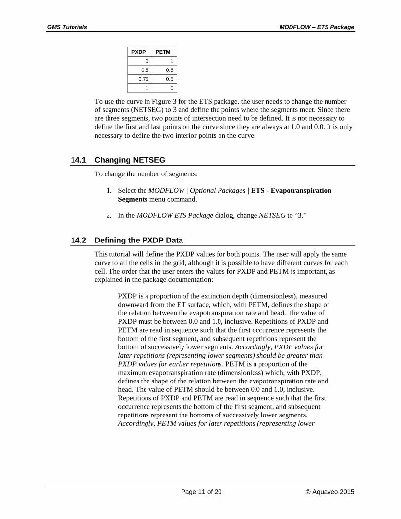
To use the curve in Figure 3 for the ETS package, the user needs to change the number

of segments (NETSEG) to 3 and define the points where the segments meet. Since there

are three segments, two points of intersection need to be defined. It is not necessary to

define the first and last points on the curve since they are always at 1.0 and 0.0. It is only

necessary to define the two interior points on the curve.

14.1 Changing NETSEG

To change the number of segments:



2. In the MODFLOW ETS Package dialog, change NETSEG to “3.”

14.2 Defining the PXDP Data

This tutorial will define the PXDP values for both points. The user will apply the same

curve to all the cells in the grid, although it is possible to have different curves for each

cell. The order that the user enters the values for PXDP and PETM is important, as

explained in the package documentation:

PXDP is a proportion of the extinction depth (dimensionless), measured

downward from the ET surface, which, with PETM, defines the shape of

the relation between the evapotranspiration rate and head. The value of

PXDP must be between 0.0 and 1.0, inclusive. Repetitions of PXDP and

PETM are read in sequence such that the first occurrence represents the

bottom of the first segment, and subsequent repetitions represent the

bottom of successively lower segments. Accordingly, PXDP values for

later repetitions (representing lower segments) should be greater than

PXDP values for earlier repetitions. PETM is a proportion of the

maximum evapotranspiration rate (dimensionless) which, with PXDP,

defines the shape of the relation between the evapotranspiration rate and

head. The value of PETM should be between 0.0 and 1.0, inclusive.

Repetitions of PXDP and PETM are read in sequence such that the first

occurrence represents the bottom of the first segment, and subsequent

repetitions represent the bottoms of successively lower segments.

Accordingly, PETM values for later repetitions (representing lower



segments) generally would be less than PETM values for earlier

repetitions.3 (emphasis added)

1. Change the View/Edit combo box to “PXDP. Curve segments.”

2. Make sure the Segment array is set to “1.” This means the user is

viewing/editing data for the first point.



5. Change the Segment array to “2” in order to view the second segment.



14.3 Defining the PETM Data

The next step is to define the PETM data for both points. Again, the user will make the

same curve apply to all the cells in the grid.

1. Change the View/Edit combo box to “PETM. Curve segments.”

2. Set the Segment array to “1.”



5. Set the Segment array to “2.”



8. Click OK to exit the MODFLOW ETS Package dialog.








The next steps are to save these changes and run MODFLOW.




The user should notice some slight changes in the new solution.

4. Compare all four solutions by alternately selecting the “modfgrid

(MODFLOW)” , the “evt (MODFLOW)” , the “ets1 (MODFLOW)” ,

and the “ets2 (MODFLOW)” items in the Project Explorer.



Before changing the model to use a conceptual model, save the model with a new name.




17 Building a Conceptual Model

The next step is to examine how to use a conceptual model with ETS data.

17.1 Creating the Conceptual Model

1. Right-click in the Project Explorer and select the New | Conceptual Model

command from the pop-up menu.

2. In the Conceptual Model Properties dialog, change the Name to “modfgrid.”

3. Click OK.

17.2 Creating a Coverage

1. Right-click on the modfgrid conceptual model the user just created in the

Project Explorer.



2. Select the New Coverage command from the pop-up menu.

3. In the Coverage Setup dialog, change the Coverage Name to “ets.”

4. In the list of Areal Properties, turn on the following options:

Max ETS rate

ETS elev.

ETS Extinction depth

ETS Segmented curve

5. Click OK to exit the Coverage Setup dialog.

17.3 Creating the Polygon

1. Select the Create Arc tool.

2. Create an arc that surrounds the grid. End the arc on the starting point by double-

clicking in order to form a closed polygon, as shown in Figure 4.

3. Select the Feature Objects | Build Polygons menu command.

Figure 4 Creating a polygon that encompasses the model grid



17.4 Setting the Polygon Properties

1. Switch to the Select tool.

2. Double-click anywhere inside the polygon that was just created.

3. In the Attribute Table dialog, set the values to be as shown in Figure 5.

Figure 5 Coverage Properties dialog showing the polygon

The value in the ETS segmented curve column is the number of an XY series. The curves

are defined using the XY Series Editor, and each XY series has a unique number. A

value of -1 indicates that no XY series has been specified yet.

4. Click on the button in the ETS segmented curve column.

This brings up the XY Series Editor.

5. Enter the following values in the XY Series Editor.

PXDP PETM

0 1

0.4 0.9

0.8 0.6

1 0

Note that these are different values than were used previously. Also, note that, in this

case, the user will include the first and last values on the curve.

6. Click OK to exit the XY Series Editor.

Notice the value in the ETS segmented curve column has changed.

7. Click OK to exit the Attribute Table dialog.



18 Map MODFLOW

The conceptual model is set up so now it is possible to map it to the MODFLOW grid.

1. Select the Feature Objects | Map MODFLOW menu command.

2. When the Map Model dialog appears, click OK.

19 Examining the ETS Package

The next step is to take a look at the data in MODFLOW that was mapped from the

conceptual model.



2. In the MODFLOW ETS Package dialog, switch the View/Edit combo box

between the various selections and check that the Elevation is “59,” the Max ET

rate is “0.01,” and the ET extinction depth is “6.”

3. Switch the View/Edit combo box to “PXDP, Curve segments.”

4. Check that the Segment array for “1” are all “0.4”

5. Check that the Segment array for “2” are all “0.8.”

6. Switch the View/Edit combo box to “PETM. Curve segments.”

7. Check that the Segment array for “1” are all “0.9.”

8. Check that the Segment array for “2” are all “0.6” for segment array 2.

9. Click OK.







4. Compare all five solutions by alternately selecting the “modfgrid (MODFLOW)”

, the “evt (MODFLOW)” , the “ets1 (MODFLOW)” , the “ets2



(MODFLOW)” , and the “ets3 (MODFLOW)” items in the Project

Explorer.



Next the user will examine how parameters work with the EVT and ETS packages, so

the user should save the model with a new name.




22 Parameters

It is possible to use parameters with the EVT and ETS packages. This tutorial will use

parameters to assign one ET rate to the left side of the model and a different rate to the

right side.

22.1 Parameterizing the Model

1. Turn off the “Map Data” item in the Project Explorer.

2. Click on the “3D Grid Data” item in the Project Explorer to switch to the 3D

grid module.

3. Select the Select Cells tool.

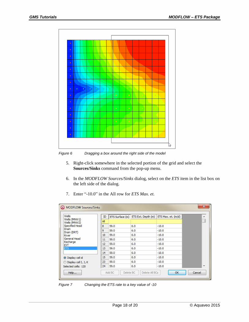
4. Drag a box around the right side of the model to select those cells as shown in

the figure below.



Figure 6 Dragging a box around the right side of the model

5. Right-click somewhere in the selected portion of the grid and select the

Sources/Sinks command from the pop-up menu.

6. In the MODFLOW Sources/Sinks dialog, select on the ETS item in the list box on

the left side of the dialog.

7. Enter “-10.0” in the All row for ETS Max. et.

Figure 7 Changing the ETS rate to a key value of -10



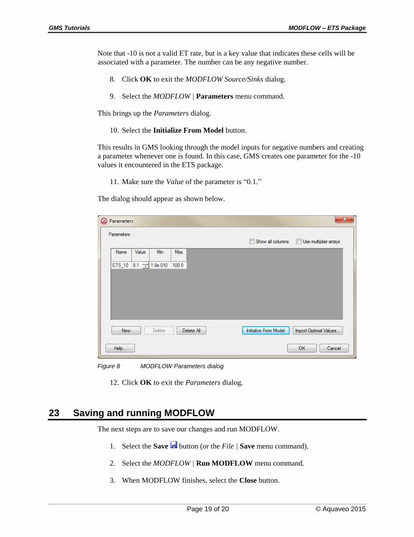
Note that -10 is not a valid ET rate, but is a key value that indicates these cells will be

associated with a parameter. The number can be any negative number.

8. Click OK to exit the MODFLOW Source/Sinks dialog.

9. Select the MODFLOW | Parameters menu command.

This brings up the Parameters dialog.

10. Select the Initialize From Model button.

This results in GMS looking through the model inputs for negative numbers and creating

a parameter whenever one is found. In this case, GMS creates one parameter for the -10

values it encountered in the ETS package.

11. Make sure the Value of the parameter is “0.1.”

The dialog should appear as shown below.

Figure 8 MODFLOW Parameters dialog

12. Click OK to exit the Parameters dialog.

23 Saving and running MODFLOW








4. Compare all five solutions by alternately selecting the “modfgrid (MODFLOW)”

, the “evt (MODFLOW)” , the “ets1 (MODFLOW)” , the “ets2

(MODFLOW)” , the “ets3 (MODFLOW)” , and the “ets4 (MODFLOW)”

items in the Project Explorer.


24 Conclusion

This concludes the tutorial. Here are the key concepts from this tutorial:

GMS supports both the EVT and ETS packages. Both packages can be used at

the same time if desired.

The ETS package produces the same results as the EVT package if only one

curve segment is defined.

ETS data can be viewed and edited in the ETS Package dialog.

The order in which the PXDP and PETM data is entered is important. PXDP

values should be in increasing order and PETM values should be in decreasing

order.

ETS data can be defined on polygons in a conceptual model.

Documents

v. 10 - Aquaveogmstutorials-10.0.aquaveo.com/MODFLOW-ETSPackage.pdf · Notice that the tutorial left NETSEG at 1. This means there is one curve segment, which This means there is