Embed Size (px)
Citation preview
2
Table of Contents Getting Started .........................................................................................................................................................3
Installation ............................................................................................................................................................3
Windows ...........................................................................................................................................................3
Linux..................................................................................................................................................................3
Running the Program ............................................................................................................................................4
Basic Geometry .........................................................................................................................................................5
Surface Cards (MCNP5 Manual Vol. II Page: 3-12) ...............................................................................................5
Macro Bodies (MCNP5 Manual Vol. II Page: 3-18) ...............................................................................................7
Cell Cards (MCNP5 Manual Vol. II Page: 3-9) .......................................................................................................7
Advanced Geometry .............................................................................................................................................. 10
Universes (MCNP5 Manual Vol. II Page: 3-26) .................................................................................................. 10
Lattices (MCNP5 Manual Vol. II Page: 3-28) ...................................................................................................... 10
Materials (MCNP5 Manual Vol. II Page: 3-122) ..................................................................................................... 12
Source Terms and Criticality (MCNP5 Manual Vol. II Page: 3-53) ......................................................................... 13
Tallies (MCNP5 Manual Vol. II Page: 3-81) ............................................................................................................ 14
Flux and Energy Tallies ...................................................................................................................................... 15
Mesh Tallies (MCNP5 Manual Vol. II Page: 3-118) ............................................................................................ 17
Burn-up (MCNPX Manual Page: 5-77) ................................................................................................................... 19
Further Study ......................................................................................................................................................... 20

3
Getting Started This section will cover basic set-up of the MCNP5/X. This involves installing the program, setting up an
environment, and running the program. If there are any questions about this process please contact me. It is
not very easy to get started with this process if you have never dealt with installing software in this way before.
Installation There are several different versions of MCNP that a person can obtain from RSICC. One can get only the
executables, the full source code, and also the newest beta release. The only reason for needing the source
code is if you plan on compiling the source code yourself to enable different options, or even to modify the
code to suit your needs. I will not discuss this here as it is not a trivial process to learn how to compile code and
set-up environment without having ever used the MCNP at all. The following will discuss how to install the ex-
ecutables, data and set the environments up. The data libraries will take a while to install as they are extremely
large files (remember back to the Brookhaven National Lab cross sections you used to look up in NE405/408,
and imagine these cross sections for different temperatures, etc. and the amount of data starts multiplying
fast). It is possible to add in new cross sections for MCNP to read if you have data from an outside source that
you’d like to use, but I will not discuss that here.
Windows
For the windows users there is a simple installation program that uses the windows install wizard to
guide you through the process. On the disk you received from RSICC you will want to go into the MCNP5 direc-
tory and then the windows installer directory and run the setup.exe file. This should guide you through the rest
of the way of installing MCNP5. The code needs cross sections to compute the nuclear interactions and there-
fore the MCNPDATA folder should be opened and similarly followed to install the data libraries.
You should now have MCNP5 and the data libraries installed. This is able to run problems now, but
there is also MCNPX that can be installed as well. MCNPX will be installed in a similar way except that the file to
install MCNPX is a windows batch file located in that directory.
Linux
NOTE: Do NOT try this if you are not experienced with what you are doing in this environment. It can
cause problems if you do not install files properly and set permissions accordingly.
The linux installation is a lot more exciting in that you are required to do some work and must know
your way around a terminal window. During the linux installation readme files will be your best friend. MCNP5
and MCNPX tell you to do things differently and don’t agree on the installation process and thus installing both
of them for the first time can be rather confusing. I would first recommend installing the data libraries some-
where that you can reference later. These libraries are used by both programs and need to be extracted only
once. An important feature is that you need to set your DATAPATH variable to wherever you installed your da-
ta libraries. This is where I prefer linux in that you can do things your own way without being forced to install
them to a directory structure you don’t like.
After installing the data libraries and setting your DATAPATH variable one can move onto the programs
themselves. For a variety of machines and set-ups there are executables that are included on the disks. These
executables need to be put into a folder for you to run from later. Note that you will have to know your com-
puter architecture etc. to choose the proper binary file.
Your system should now have a folder with binary executables and also a location storing all the data
libraries. The next step is to set all the environment variables that you will need. The location that the executa-
ble files are located should be added to your PATH variable. This will now allow MCNP5/X to be executed. To
visualize the geometry for MCNP an x-windows server is required. To set this up you will need to set your DIS-
PLAY variable up properly to an output for an x-window. These three variables (DATAPATH, PATH, DISPLAY),
are the three variables that you will need almost every time you want to run MCNP and thus I would recom-
mend putting these in your profile so that they will be around every time you run your machine.

4
Running the Program The first thing that I will mention is that the User’s Manuals are extremely helpful. These manuals have
loads of information in them and can help you through the entire process that this tutorial takes you through.
They are very dense though and it is helpful to know what you are looking for before beginning to read 500+
pages from a manual, which is what I will try and help with.
You should now have an executable version of MCNP and data libraries installed. The next step now is
getting the program to actually run. This is done by executing the program through a command prompt if
you’re on windows, or by executing the binary file on a linux machine. To run a problem the basic syntax is:
mcnp5 i=filename options
where ‘i’ is short for ‘inp’ and indicates to look for the given input file. This can also be replaced by ‘n’ which
will label all files the same way. For example, let’s say my input file is named test. I could run the program like
this:
mcnp5 i=test
which produces a file called outp, and several others with the data from the problem. Each subsequent run
with the syntax like this will produce new output files with the last letter changed (outq, outr, …). If instead I
ran the program like this:
mcnp5 n=test
which produces a file called testo, and several other test(…) files. This is helpful if you have several input files
and want to separate the output in a unique way. The drawback here is that if the output files already exist the
program will terminate without executing.
The options available for running your problem allow you to process different aspects of the execution
in a unique order. If no options are specified (as above) then the default options are given to the program,
which are: ixr
The options are as follows:
i=process input file
p=plot geometry (with the built-in plotter, NOT vised)
x=process cross sections
r=transport the particles (run the program)
z=plot tally results or cross section data
You can see that the default of ‘ixr’ will first process the input file, then process the cross sections that are
needed for the problem and finally transport the particles specified in the problem. Another typical option that
I use frequently in my executions is ‘ip’. This will process the input and then plot the geometry. I personally pre-
fer this plotter to vised, but each person has their own personal preferences.

5
Basic Geometry In MCNP every input file contains three sections, which are: cell cards, surface cards and data cards.
The geometry is only concerned with the cell and surface cards. Cell cards are used to specify volumes, and sur-
face cards are obviously used to specify the surfaces that enclose the volumes. MCNP allows the user many
different options of specifying the different parameters, but does require an order to every input file. The
layout for an input file is as follows: Cell cards followed by a blank line, then surface cards followed by a blank
line, then the data cards followed by a blank line.
A typical input file looks something like this:
c Cell Cards
... Different cells that are specified
[blank line]
c Surface Cards
... Different surfaces that are specified
[blank line]
c Data Cards
... Any data that is needed for the problem
[blank line]
Every file is organized in that way, but the way that you specify the individual components can vary based on
personal preferences and ease of specifying different geometries. One note is that MCNP does not allow any
blank lines other than one after the three sections. This means that if you want your input file to be more read-
able you will have to put a 'c' at the beginning of the line to indicate that the line is commented (This shows the
Fortran heritage of the code).
Surface Cards (MCNP5 Manual Vol. II Page: 3-12) Parameters and options: j n a
j = surface number integer value from 1-99999
n = coordinate transformation information
a = equation mnemonic
Surfaces are objects that can be combined in unique ways to create enclosed volumes, which we discovered in
the cell cards. There are many different surface types listed in the manual that one is able to use, and I will
briefly introduce a plane. A common plane equation is this Ax+By+Cz+D=0
To specify this plane surface in MCNP the following would be used: j p A B C D
where j is the surface number, p indicates that it is the equation of a plane and A, B, C, D are the plane parame-
ters. To create a surface parallel to the Z axis at a height of 5 the following two lines could be used:
j pz 5
j p 0 0 1 5
6
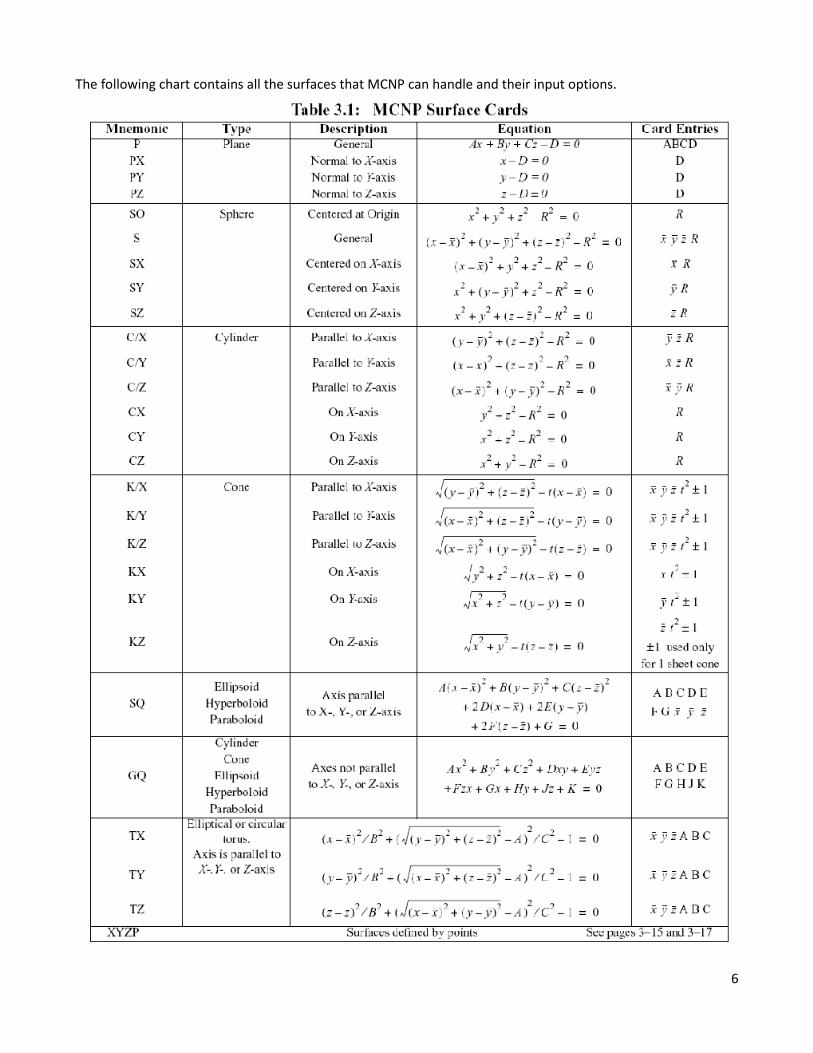
The following chart contains all the surfaces that MCNP can handle and their input options.
7
Macro Bodies (MCNP5 Manual Vol. II Page: 3-18) Another way to specify multiple surfaces at once is with the use of macro bodies. Macro bodies are simply
combinations of multiple surfaces that MCNP has already predefined. One such macro body is a box. The
mnemonic for creating a box is the following:
BOX Vx Vy Vz A1x A1y A1z A2x A2y A2z A3x A3y A3z
where the V's are the coordinates of a corner and the A's are the vector's of the sides leaving that corner. De-
pending on the math that you use to create your volumes it could be advantageous to use macro bodies as a
quicker method of specifying many surfaces. The standard way of specifying six surfaces and combining these
with cell cards to create a box is valid as well, and this method of specifying every surface will be used in all the
examples.
Cell Cards (MCNP5 Manual Vol. II Page: 3-9) Parameters and options: j m [d] geometry parameters
j=cell number (1-99999)
m=number of material card (0 if void)
d=density if a material is present (nothing if void)
geometry=definition of how surfaces are arranged
parameters=optional input to specify importances, universes etc. which will be discussed later
In the geometry section surfaces that are used in this cell (think volume) are listed, which includes how these
surfaces interact with each other. Surfaces have a negative and positive sense to them that one can talk about.
The positive sense is the side of the surface that is pointing 'toward' the positive axes. A plane with the equa-
tion z=0 (xy plane) has orientation with a negative side below the xy plane and positive side above the xy plane.
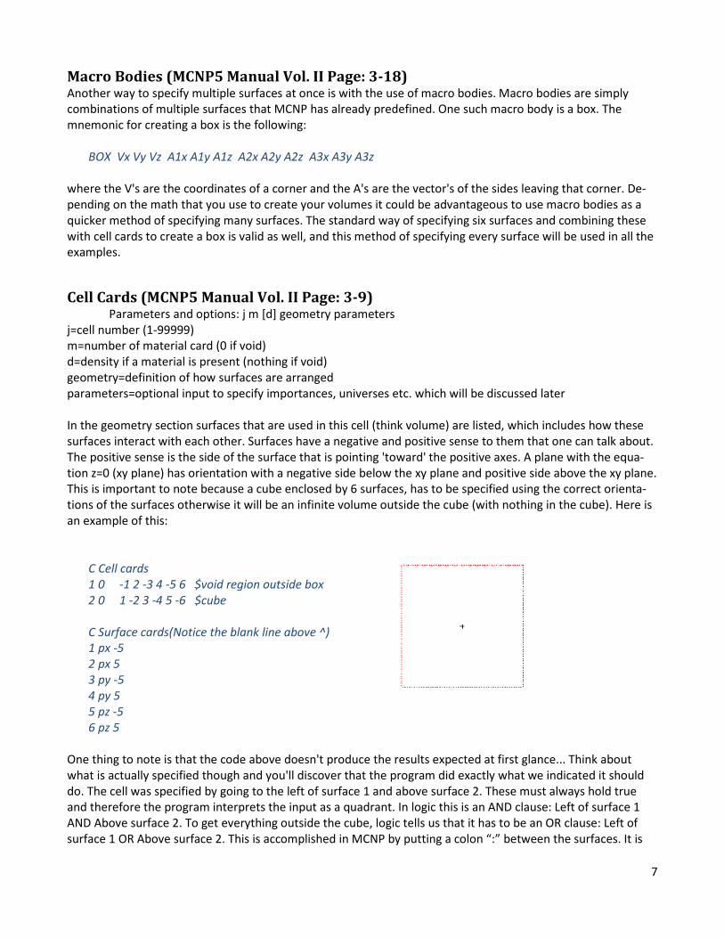
This is important to note because a cube enclosed by 6 surfaces, has to be specified using the correct orienta-
tions of the surfaces otherwise it will be an infinite volume outside the cube (with nothing in the cube). Here is
an example of this:
C Cell cards
1 0 -1 2 -3 4 -5 6 $void region outside box
2 0 1 -2 3 -4 5 -6 $cube
C Surface cards(Notice the blank line above ^)
1 px -5
2 px 5
3 py -5
4 py 5
5 pz -5
6 pz 5
One thing to note is that the code above doesn't produce the results expected at first glance... Think about
what is actually specified though and you'll discover that the program did exactly what we indicated it should
do. The cell was specified by going to the left of surface 1 and above surface 2. These must always hold true
and therefore the program interprets the input as a quadrant. In logic this is an AND clause: Left of surface 1
AND Above surface 2. To get everything outside the cube, logic tells us that it has to be an OR clause: Left of
surface 1 OR Above surface 2. This is accomplished in MCNP by putting a colon “:” between the surfaces. It is
8
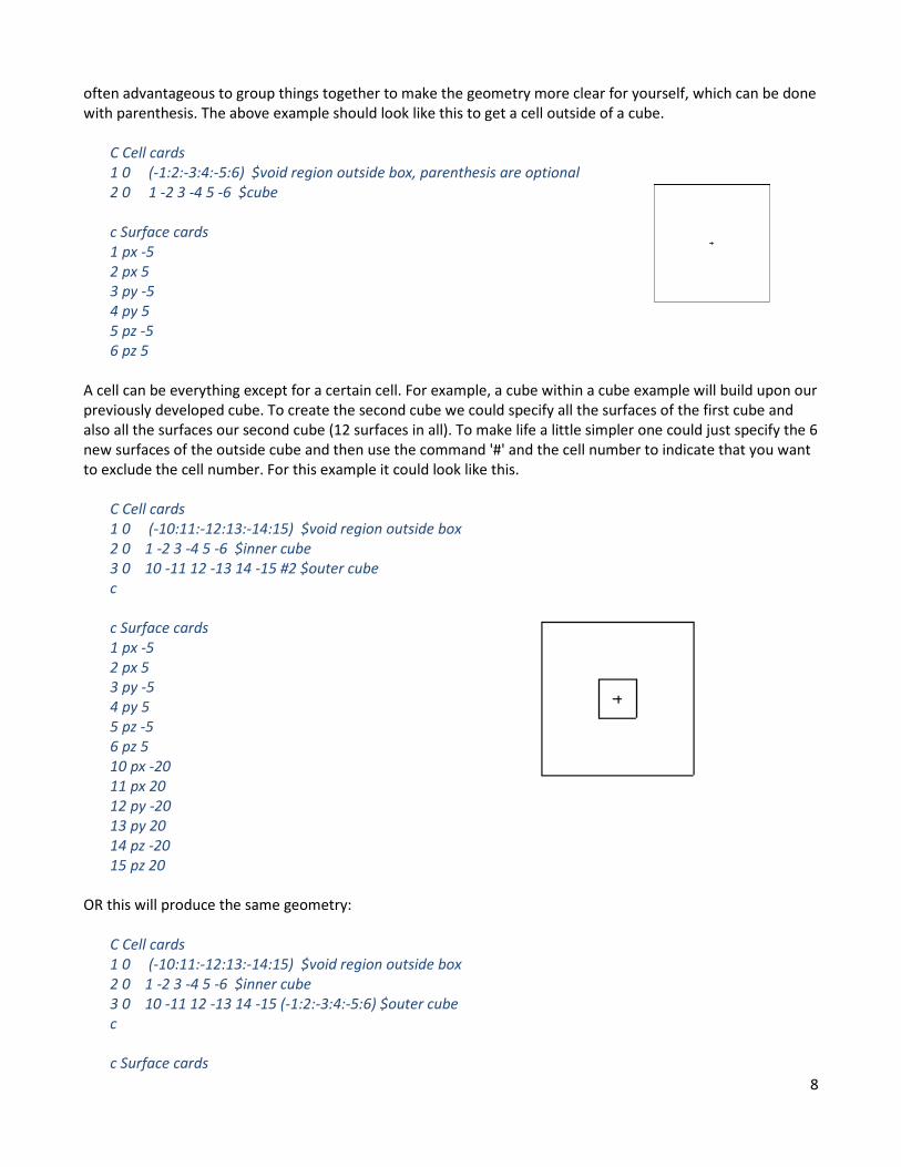
often advantageous to group things together to make the geometry more clear for yourself, which can be done
with parenthesis. The above example should look like this to get a cell outside of a cube.
C Cell cards
1 0 (-1:2:-3:4:-5:6) $void region outside box, parenthesis are optional
2 0 1 -2 3 -4 5 -6 $cube
c Surface cards
1 px -5
2 px 5
3 py -5
4 py 5
5 pz -5
6 pz 5
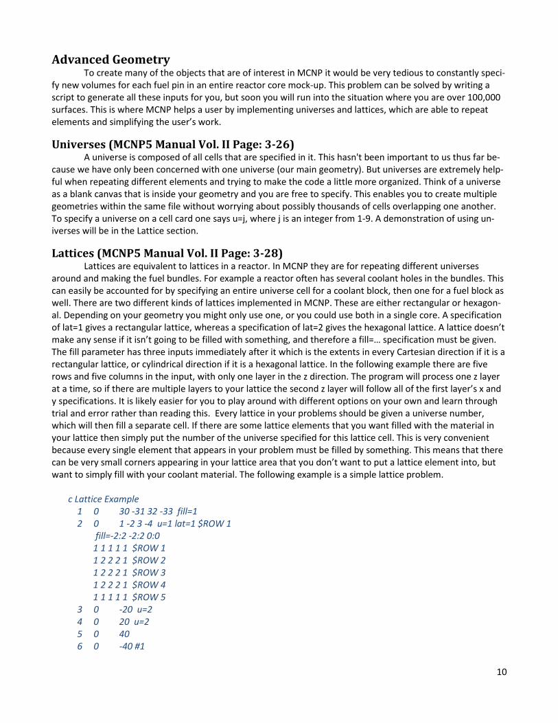
A cell can be everything except for a certain cell. For example, a cube within a cube example will build upon our
previously developed cube. To create the second cube we could specify all the surfaces of the first cube and
also all the surfaces our second cube (12 surfaces in all). To make life a little simpler one could just specify the 6
new surfaces of the outside cube and then use the command '#' and the cell number to indicate that you want
to exclude the cell number. For this example it could look like this.
C Cell cards
1 0 (-10:11:-12:13:-14:15) $void region outside box
2 0 1 -2 3 -4 5 -6 $inner cube
3 0 10 -11 12 -13 14 -15 #2 $outer cube
c
c Surface cards
1 px -5
2 px 5
3 py -5
4 py 5
5 pz -5
6 pz 5
10 px -20
11 px 20
12 py -20
13 py 20
14 pz -20
15 pz 20
OR this will produce the same geometry:
C Cell cards
1 0 (-10:11:-12:13:-14:15) $void region outside box
2 0 1 -2 3 -4 5 -6 $inner cube
3 0 10 -11 12 -13 14 -15 (-1:2:-3:4:-5:6) $outer cube
c
c Surface cards

9
1 px -5
2 px 5
3 py -5
4 py 5
5 pz -5
6 pz 5
10 px -20
11 px 20
12 py -20
13 py 20
14 pz -20
15 pz 20
10
Advanced Geometry To create many of the objects that are of interest in MCNP it would be very tedious to constantly speci-
fy new volumes for each fuel pin in an entire reactor core mock-up. This problem can be solved by writing a
script to generate all these inputs for you, but soon you will run into the situation where you are over 100,000
surfaces. This is where MCNP helps a user by implementing universes and lattices, which are able to repeat
elements and simplifying the user’s work.
Universes (MCNP5 Manual Vol. II Page: 3-26) A universe is composed of all cells that are specified in it. This hasn't been important to us thus far be-
cause we have only been concerned with one universe (our main geometry). But universes are extremely help-
ful when repeating different elements and trying to make the code a little more organized. Think of a universe
as a blank canvas that is inside your geometry and you are free to specify. This enables you to create multiple
geometries within the same file without worrying about possibly thousands of cells overlapping one another.
To specify a universe on a cell card one says u=j, where j is an integer from 1-9. A demonstration of using un-
iverses will be in the Lattice section.
Lattices (MCNP5 Manual Vol. II Page: 3-28) Lattices are equivalent to lattices in a reactor. In MCNP they are for repeating different universes
around and making the fuel bundles. For example a reactor often has several coolant holes in the bundles. This
can easily be accounted for by specifying an entire universe cell for a coolant block, then one for a fuel block as
well. There are two different kinds of lattices implemented in MCNP. These are either rectangular or hexagon-
al. Depending on your geometry you might only use one, or you could use both in a single core. A specification
of lat=1 gives a rectangular lattice, whereas a specification of lat=2 gives the hexagonal lattice. A lattice doesn’t
make any sense if it isn’t going to be filled with something, and therefore a fill=… specification must be given.
The fill parameter has three inputs immediately after it which is the extents in every Cartesian direction if it is a
rectangular lattice, or cylindrical direction if it is a hexagonal lattice. In the following example there are five
rows and five columns in the input, with only one layer in the z direction. The program will process one z layer
at a time, so if there are multiple layers to your lattice the second z layer will follow all of the first layer’s x and
y specifications. It is likely easier for you to play around with different options on your own and learn through
trial and error rather than reading this. Every lattice in your problems should be given a universe number,
which will then fill a separate cell. If there are some lattice elements that you want filled with the material in
your lattice then simply put the number of the universe specified for this lattice cell. This is very convenient
because every single element that appears in your problem must be filled by something. This means that there
can be very small corners appearing in your lattice area that you don’t want to put a lattice element into, but
want to simply fill with your coolant material. The following example is a simple lattice problem.
c Lattice Example
1 0 30 -31 32 -33 fill=1
2 0 1 -2 3 -4 u=1 lat=1 $ROW 1
fill=-2:2 -2:2 0:0
1 1 1 1 1 $ROW 1
1 2 2 2 1 $ROW 2
1 2 2 2 1 $ROW 3
1 2 2 2 1 $ROW 4
1 1 1 1 1 $ROW 5
3 0 -20 u=2
4 0 20 u=2
5 0 40
6 0 -40 #1
11
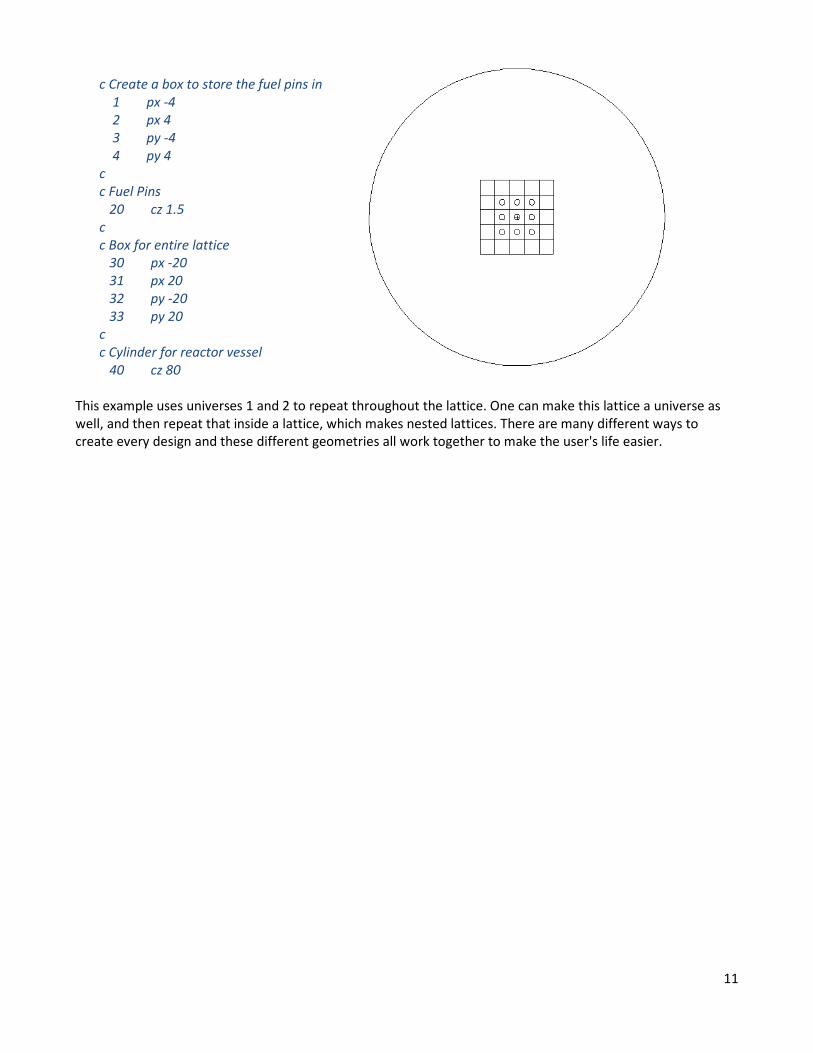
c Create a box to store the fuel pins in
1 px -4
2 px 4
3 py -4
4 py 4
c
c Fuel Pins
20 cz 1.5
c
c Box for entire lattice
30 px -20
31 px 20
32 py -20
33 py 20
c
c Cylinder for reactor vessel
40 cz 80
This example uses universes 1 and 2 to repeat throughout the lattice. One can make this lattice a universe as
well, and then repeat that inside a lattice, which makes nested lattices. There are many different ways to
create every design and these different geometries all work together to make the user's life easier.

12
Materials (MCNP5 Manual Vol. II Page: 3-122) Parameters and options: Mn ZAID1 fraction1 ZAID2 fraction2
n= material number (used to identify materials in cell cards)
ZAID= ZZZAAA of the isotope (for U-238 it looks like 92238)
fraction=decimal percent of the given isotope
Materials are put in the data cards of the MCNP input file. These are specified using the MAT card, and
indicating what material you want to import or create. One can create H2O or use the libraries existing water
entry. If you have knowledge of the composition of a certain material, like cement, then you can give either
weight% or atom% for the isotopes in the material and MCNP will use this for the cross sections when that ma-
terial is used in the cell cards. To specify that atom% is used a positive decimal must be given after the ZAID,
and to use weight% then put a negative sign in front of the decimal. This is a critical piece of information for
MCNP and specifying the wrong isotope in a material can really screw up calculations due to the significantly
different cross sections. A typical MAT card is given below for B4C.
C natural elements of B4C can be specified by using an AAA of 000
M1 05000 0.8 06000 0.2
In B4C, the main absorber is B10. Many control rods will be enriched in their B10 content, and to do this you can
specify what isotopic content you want for each material.
C B4C enriched with 75% B10
M1 05010 0.6 05011 0.2 06000 0.2

13
Source Terms and Criticality (MCNP5 Manual Vol. II Page: 3-53) In every criticality problem a KCODE card is required. This card is used to specify how statistically signif-
icant the problem you have will be. The most important thing to note here is that you want to be positive that
you are skipping enough runs initially to let the source neutrons settle across the core. This will yield random
locations for the source neutrons in each generation to ensure good statistics. If one does not skip enough
cycles the source neutrons will be preferentially located near your initial source location. One simple way to
test for this is to run a sample problem and see when the estimated k value settles out and doesn’t jump
around very much and then skip all the trials before that.
Parameters and options: KCODE NSRCK RKK IKZ KCT
NSRCK= number of source histories per cycle (how many neutrons to follow)
RKK= initial keff guess
IKZ= number of cycles to skip
KCT= number of active cycles to use (after the skipped cycles)
All of these options will vary depending on the problem you are dealing with. Very large problems will require a
lot of source histories, and a lot of cycles to skip before they will settle, while a small core could be very small
numbers to obtain good statistics.
Now that all the source cycles are specified the locations of the initial source particles must be input.
This can be done in many different ways, but I will cover the two easiest and most common ways of doing this.
An SDEF card creates a source definition. This can be a surface, or cell and you are able to give the particles a
specific energy, direction, and many other unique options. This is a very versatile way of specifying a source
and is generally used in shielding problems and non-criticality problems.
Parameters and options: SDEF many options…
There are many different options that you can specify on the SDEF card, for all of these I will refer you to
MCNP5 Manual Volume II: Page 3-55. Study these options carefully if you choose to use this type of source as
there are many different ways to specify the same initial conditions.
Another option to specify the initial source locations is to use a KSRC card. This is a very simple way of
specifying the initial neutron locations. The KSRC card samples from a Watt fission distribution for energy, so
there is no need to specify your own energy distribution, and will also place particles randomly at all the loca-
tions specified in the card.
Parameters and options: KSRC x1 y1 z1 x2 y2 z2
x, y, z= x, y, z locations of the initial source neutrons
For the entire initial source distribution used with the KCODE card you must have at least one initial
location be in a fissile region. This means that some math will need to be done to figure out the x, y, and z loca-
tions of the fissile regions if a KSRC is used, and if an SDEF card is used you will need to ensure that you are
placing the source in a fissile region.
When beginning your criticality calculations I would recommend beginning with the KSRC initial loca-
tions as they are somewhat easier to understand and implement. An example of these criticality cards follows.
c There are 5000 initial neutrons with an initial keff guess of 1
c Skipping 20 cycles at the beginning and then conducting 40 active cycles
c making a total of 60 cycles that the program will run
c There are 5 locations where the first cycle neutrons can originate from
KCODE 5000 1.0 20 40
KSRC 0 0 250 25 25 250 -25 -25 250 25 -25 250 -25 25 250
14
Tallies (MCNP5 Manual Vol. II Page: 3-81) All of the information up to this point should enable you to run the program and produce the generic
output that MCNP gives you. Of course this is not sufficient for the desires of designing a full scale core. When
designing the core, we have to take into account the heat that is in the coolant and pins, make sure that the
flux is a reasonable value in the core, check the doses outside the containment area, and many other things. To
obtain extra data beyond what the core program gives you MCNP gathers information using data cards called
tallies. Tallies are able to be computed over surfaces, cells, and at points. MCNP also lets you look at individual
pins to find out the specific heating within a single pin or channel, or allows you to average a tally over the en-
tire core to visualize what the average heating is across the core. This allows for a myriad of options and a lot of
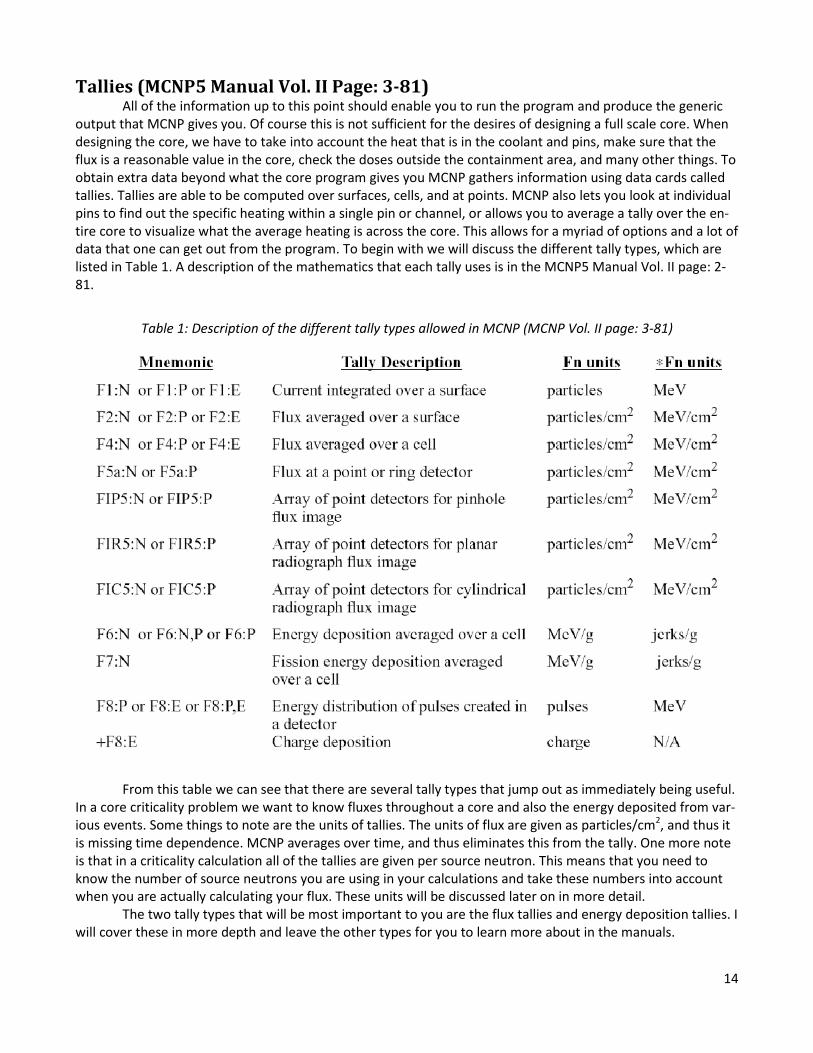
data that one can get out from the program. To begin with we will discuss the different tally types, which are
listed in Table 1. A description of the mathematics that each tally uses is in the MCNP5 Manual Vol. II page: 2-
81.
Table 1: Description of the different tally types allowed in MCNP (MCNP Vol. II page: 3-81)
From this table we can see that there are several tally types that jump out as immediately being useful.
In a core criticality problem we want to know fluxes throughout a core and also the energy deposited from var-
ious events. Some things to note are the units of tallies. The units of flux are given as particles/cm2, and thus it
is missing time dependence. MCNP averages over time, and thus eliminates this from the tally. One more note
is that in a criticality calculation all of the tallies are given per source neutron. This means that you need to
know the number of source neutrons you are using in your calculations and take these numbers into account
when you are actually calculating your flux. These units will be discussed later on in more detail.
The two tally types that will be most important to you are the flux tallies and energy deposition tallies. I
will cover these in more depth and leave the other types for you to learn more about in the manuals.
15
Flux and Energy Tallies Parameters and options: Fn:pl S1 S2 (S3 … S4) T
n= tally number (the ones digit determines the tally type, i.e. F1, F11, F311 will all be a current tally)
pl= particle type (N=neutrons, P=photons, E=electrons, N,P=neutrons and photons)
S1= surface or cell that you want the tally over, parentheses indicate an average over all cells/surfaces enclosed
T= optional average over all previously specified surfaces and cells (eliminates you rewriting all your numbers)
To obtain a tally of interest you have to know what each of your cell numbers or surfaces correspond to
in your core. For example, a typical core will have several different fuel pins of different enrichment types.
These different pins are different cells, and if you want to know the heating of all the pins you must specify all
the different cells possible. A simple flux tally looks like the following.
C neutron tally over cells 1, 2, and 3, plus an average over cells 1, 2, and 3
F14:N 1 2 3 T
C this is equivalent to the following specification
F24:N 1 2 3 (1 2 3)
Each of those examples generates four tally outputs. A typical core involves universes and lattices to repeat the
cells. This means that there could be many cell 1’s in the problem geometry, but you may only want a single pin
to know the peak power pin. MCNP of course has special syntax to go inside of lattices and pick out specific
elements.
Parameters and options: Fn:pl S1 (S2 S3) < (C4 C5) < C6[I1 I2]
n= tally number (the ones digit determines the tally type, i.e. F1, F11, F311 will all be a current tally)
pl= particle type (N=neutrons, P=photons, E=electrons, N,P=neutrons and photons)
S1= surface or cell that you want the tally over, parentheses indicate an average over all cells/surfaces enclosed
C1=cell number containing a filled universe or U=# where # is the universe number
I1=range of lattice positions desired
< indicates that you only want a tally when the items on the left occur in the cell(s) on the right
This is likely confusing right now so I’ll try and give some simple examples here. If we have cell 1 con-
tained inside of cells 2 and 3 (cells 2 and 3 must both be universes), and we would like to tally cell 1 ONLY when
it occurs inside of cell 2 the following could be used.
F4:N (1 < 2)
Now let’s say that cell 2 is contained inside of cell 10, which is a repeated lattice. Now I only want to know the
center lattice element’s flux. Expand upon the previous example as follows.
F4:N (1 < 2 < 10[0 0 0])
If this seems abstract, visualize cell one being the UO2 of the fuel pin. Cell 2 is a universe that contains the UO2
cladding, plenum, and anything else you choose to include. Cell 10 is then a fuel assembly containing many dif-
ferent pins, and we simply want the one located at position (0,0,0).
Another thing to note is how many tally bins you are creating when using this nested syntax.
F4:N (1 < 2 3 < 10[0 0 0]) $this has two tally bins, cell 1 inside cell 2 and cell 1 inside cell 3

16
This is equivalent to:
F4:N (1 < 2 < 10[0 0 0]) (1 < 3 < 10[0 0 0])
To get only one tally bin the following can be used:
F4:N (1 < (2 3) < 10[0 0 0]) $gives one tally bin for when cell 1 occurs inside of cell 2 OR cell 3
One can also use U=# to specify a given universe rather than using a specific cell number. This syntax
can be easier to remember, but you can run into problems when there are multiple cells inside the universe,
and end up creating 1000’s of tally bins on accident because you didn’t enclose the universe in parentheses.
The MCNP5 Manual Vol. II page: 3-94 explains how to use the U=# method well.
When using repeated structures and using the same cell multiple times throughout our geometry,
MCNP needs some help calculating the volumes that you desire. This is an extremely important piece of infor-
mation as the data is normalized by the volume for the tallies and an incorrect number here will give you a
wrong final result. The SD card is used to specify volumes as follows.
Parameters and options: SDn V1 V2
n= the tally number that the volumes should correspond to
V1= volume of the first tally bin, second tally bin up to the number of bins in the problem
This will require you to do some work by hand in knowing your pin dimensions, coolant channel dimen-
sions, how many pins you have, etc. Make sure you are using the proper heights for the corresponding tallies.
For example, that your fuel is so many cm tall, and your total pin height is actually higher because of plenum
and clad. Thus is your tally over your fuel, or is it over an entire pin?
Another set of cards that may be of interest are the tally multiplier card, FM, and also the dose energy
and dose function cards, DE and DF. All of these modify the tally output in some way to yield a different result.
The FM card is used to multiply all the tally bins by a specified constant. This is to reduce the amount of post
processing you will have to do later on.
Parameters and options: FMn (bin set 1) (bin set 2)
n= tally number the multiplier corresponds to
(bin set 1)= the constant that is multiplied to the first tally bin
To multiply every bin in tally 14 by Avogadro’s number the following can be used.
F14:N (3 < 4) 3
FM14 6.022E23
The dose energy and dose function cards must be used together. The dose energy card gives the differ-
ent cut-offs for energy groups that you are interested in. This is then accompanied by the dose function card,
which gives a certain dose response based on the energy group. There are ICRP tables and dose functions in
the appendices of the manual to assist with the dose responses.
Parameters and options: DEn E1 E2 …
DFn F1 F2 …
n= corresponding tally number
E1= First energy cut-off
F1= First dose function cut-off
17
Mesh Tallies (MCNP5 Manual Vol. II Page: 3-118) You may have noticed that the tallies discussed thus far can give us an average flux over the core, or
even the flux in a single pin, but it isn’t able to easily produce the shape of the flux throughout the core. Often
you want to know what effect the control pins have when they are inserted, and if they depress the flux in the
proper way. To do these things there is a super-imposed mesh tally that can be done called an FMESH in
MCNP5, and RMESH in MCNPX. This tally allows you to specify how many points you want to evaluate in all
three dimensions. This allows for some very interesting data generation and plotting capabilities.
Parameters and options: FMESHn:pl GEOM=geo ORIGIN=O,O,O imesh=iii iints=III jmesh=jjj jints=JJJ
kmesh=kkk kints=KKK
n=tally number (can only be tally type 4)
pl= particle type, N, P or E
geo=xyz for rectangular coordinates, or cyl for cylindrical coordinates
O,O,O=x,y,z coordinates of the beginning of your mesh.
iii= locations of coarse mesh points in the x direction if rectangular, or r direction if cylindrical
III= number of fine mesh points that will go between every coarse mesh point listed in iii
jjj= locations of coarse mesh points in the y direction if rectangular, or theta direction if cylindrical
JJJ= number of fine mesh points that will go between every coarse mesh point listed in jjj
kkk= locations of coarse mesh points in the z direction for both rectangular and cylindrical
KKK= number of fine mesh points that will go between every coarse mesh point listed in kkk
There are also several other options that are available listed on page 3-118, but these options will ena-
ble you to get results and valuable information in a simplified manner. Setting up an FMESH tally is setting up a
new geometry on top of the current one you already have, hence the super-imposed mesh tally name. This al-
lows for a wide selection of mesh points at various areas in the geometry, rather than relying on predefined
surfaces and cells. A simple example to get a flux spectrum throughout a core is this. Analyze this before read-
ing the next paragraph and determine what you think the results will produce.
FMESH34:n GEOM=xyz ORIGIN= -75 -75 200
IMESH= 75 IINTS= 40
JMESH= 75 JINTS= 40
KMESH= 300 KINTS= 1
This definition sets up tally number 34, as a neutron flux tally. The origin for the mesh is at -75 in the x and y
directions, and 200 in the z direction. The imesh label is a coarse mesh point that is located at 75 in the x direc-
tion (we are in rectangular geometry). There are also 40 fine mesh points that will go between the origin and
the coarse mesh point listed in evenly spaced intervals. The same case applies to the y direction as in the x di-
rection. In the z direction it is a little interesting because there is only one fine mesh point listed and one coarse
mesh point listed as well. MCNP will put a single mesh point in the center of these two positions, so this geo-
metry has a z mesh point at z=250. This effectively gives us a 40x40x1 mesh or a two dimensional mesh grid at
z=250. If you implement this, you are able to obtain the actual flux shapes of different situations.
18
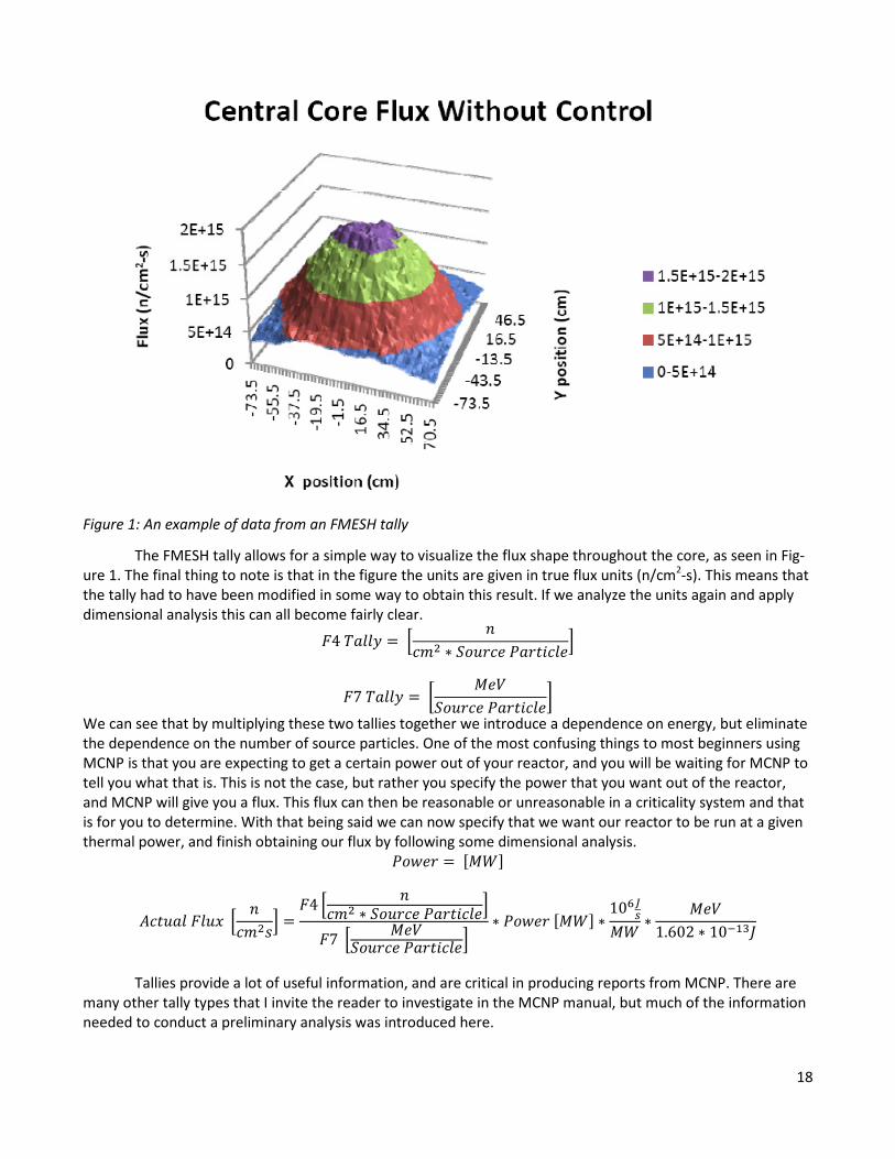
Figure 1: An example of data from an FMESH tally
The FMESH tally allows for a simple way to visualize the flux shape throughout the core, as seen in Fig-
ure 1. The final thing to note is that in the figure the units are given in true flux units (n/cm2-s). This means that
the tally had to have been modified in some way to obtain this result. If we analyze the units again and apply
dimensional analysis this can all become fairly clear.
�4 ����� � �� � ������ ���������
�7 ����� � � ��������� ���������
We can see that by multiplying these two tallies together we introduce a dependence on energy, but eliminate
the dependence on the number of source particles. One of the most confusing things to most beginners using
MCNP is that you are expecting to get a certain power out of your reactor, and you will be waiting for MCNP to
tell you what that is. This is not the case, but rather you specify the power that you want out of the reactor,
and MCNP will give you a flux. This flux can then be reasonable or unreasonable in a criticality system and that
is for you to determine. With that being said we can now specify that we want our reactor to be run at a given
thermal power, and finish obtaining our flux by following some dimensional analysis.
����� � ���
!����� ���" �� #� �
�4 �� � ������ ���������
�7 ��������� ���������
� ����� ��� � 10&'(
�� � ���1.602 � 10,-./
Tallies provide a lot of useful information, and are critical in producing reports from MCNP. There are
many other tally types that I invite the reader to investigate in the MCNP manual, but much of the information
needed to conduct a preliminary analysis was introduced here.

19
Burn-up (MCNPX Manual Page: 5-77) Burn-up of the fuel is one of the most important aspects for determining economic output of the reac-
tor, and could be a driving factor in the design of some of the new reactors that have to be run in remote areas
for 10+ years without a refueling. These constraints of the project are heavily emphasized in the initial design
phase and the final phase of gathering results, but burn-up does not play a large role in the central design por-
tion of the project. For this reason I have included burn-up as the last thing to cover in this tutorial. By this
point you should have a fully working model and realize what all of the information you are getting out pertains
too. The burn card can only be implemented with MCNPX, and is not in MCNP5. If you have been using MCNP5
for most of your calculations thus far this could produce some slight problems with syntax. Some tally identifi-
ers and other cards are different between MCNP5 and MCNPX. I would recommend running the burn-up with
everything but the geometry turned off to eliminate some of these errors. With that being said the burn card is
implemented as follows.
Parameters and options: burn time=t1 t2 ti power=P mat=m1 m2 mi matvol=MV1 MV2 MVi
omit= m1 n1 j11 j12 … j1n1 m2 n2 j21 j22 … j2n2
ti= time step from previous burn-up calculation in days. 100 100 will give a total burn-up over 200 days.
P= power in MW that the reactor is going to be run at.
mi= materials that you want burned in the problem
MVi= volume of the material specified in the problem. This is necessary if using lattices because MCNPX doesn’t
calculate your volumes for you, but I would recommend it for all materials being used and not just lattices.
OMIT – Used to omit isotopes that don’t have information associated with them
mi= material to omit isotopes from
ni= number of isotopes to omit from the material
jini= ZAID of isotope to omit from the material
The burn card can be very complicated to use, and to simplify some of the options I gave a summary of
only the most important parameters associated with the burn card. If you would like to obtain some other in-
formation or find out about all the capabilities of the burn card I invite you to read more in the manual about
this. A quick example of implementation for the burn card is as follows. Try to figure out what it is doing before
reading the next paragraph.
burn TIME=100 10R
POWER=150
MAT=1
MATVOL=951620.33
OMIT=1,6,06014,07016,08018,09018,90234,91232
The example burns 11 times, for a total of 1100 days at 100 day increments. It is run at a power of
150MW thermal throughout the 1100 days. There is only one material being burned, and it is labeled m1 in the
material cards. The total volume of material 1 in the problem is 951,620.33cc. This is specified because MCNPX
doesn’t calculate the volumes of lattices and repeated cells. The omit card tells us a lot about the problem and
the types of materials that are being used. The 1 signifies that material one needs some isotopes omitted from
the tracking. The 6 tells us how many isotopes are going to be listed. After that we can see the many different
ZAID’s of the isotopes, such as nitrogen and oxygen. Some of these may not be obvious to eliminate right away,
and thus if the burn card runs into issues tracking certain isotopes an error message will be printed telling you
exactly which isotope it can’t track, and then you can simply add that to the omit card. Make sure that the iso-
tope is not going to be critical to your calculations; otherwise you will have to do some calculations by hand to
generate final inventories of isotopes.

20
Further Study This tutorial has introduced the basic concepts and syntax to generating problems with MCNP. This
should enable you to find out more information by consulting the manual and demonstrate the usefulness of
the manual in troubleshooting your problems. To test yourself and knowledge, and possibly discover more
about lattices and criticality problems the MCNP criticality primer (contained on RSICC’s CD) has some excellent
examples to represent repeating cells. I would recommend everyone running criticality problems to at least
peruse this file to see if they could benefit from it.
MCNP5 and MCNPX are both constantly being updated and have very active groups associated with be-
ta testing, and trying to fix bugs. You can join these beta user groups by going to the homepages of the codes.