UvA-DARE (Digital Academic Repository) The X-ray outburst ... · UvA-DARE is a service provided by the library of the University of Amsterdam () UvA-DARE (Digital Academic Repository)

UvA-DARE is a service provided by the library of the University of Amsterdam (http://dare.uva.nl)

UvA-DARE (Digital Academic Repository)

The X-ray outburst of the Galactic Centre magnetar SGR J1745-2900 during the first 1.5 yearCoti Zelati, F.; Rea, N.; Papitto, A.; Viganò, D.; Pons, J.A.; Turolla, R.; Esposito, P.; Haggard,D.; Baganoff, F.K.; Ponti, G.; Israel, G.L.; Campana, S.; Torres, D.F.; Tiengo, A.; Mereghetti,S.; Perna, R.; Zane, S.; Mignani, R.P.; Possenti, A.; Stella, L.Published in:Monthly Notices of the Royal Astronomical Society

DOI:10.1093/mnras/stv480

Link to publication

Citation for published version (APA):Coti Zelati, F., Rea, N., Papitto, A., Viganò, D., Pons, J. A., Turolla, R., ... Stella, L. (2015). The X-ray outburst ofthe Galactic Centre magnetar SGR J1745-2900 during the first 1.5 year. Monthly Notices of the RoyalAstronomical Society, 449(3), 2685-2699. DOI: 10.1093/mnras/stv480

General rightsIt is not permitted to download or to forward/distribute the text or part of it without the consent of the author(s) and/or copyright holder(s),other than for strictly personal, individual use, unless the work is under an open content license (like Creative Commons).

Disclaimer/Complaints regulationsIf you believe that digital publication of certain material infringes any of your rights or (privacy) interests, please let the Library know, statingyour reasons. In case of a legitimate complaint, the Library will make the material inaccessible and/or remove it from the website. Please Askthe Library: http://uba.uva.nl/en/contact, or a letter to: Library of the University of Amsterdam, Secretariat, Singel 425, 1012 WP Amsterdam,The Netherlands. You will be contacted as soon as possible.

Download date: 07 Feb 2019

https://doi.org/10.1093/mnras/stv480

http://dare.uva.nl/personal/pure/en/publications/the-xray-outburst-of-the-galactic-centre-magnetar-sgr-j17452900-during-the-first-15-year(58f26bfc-67ea-4898-8e3f-7d09b8956932).html

MNRAS 449, 2685–2699 (2015) doi:10.1093/mnras/stv480

The X-ray outburst of the Galactic Centre magnetar SGR J1745−2900during the first 1.5 year

F. Coti Zelati,1,2,3‹ N. Rea,2,4 A. Papitto,4 D. Vigano,4 J. A. Pons,5 R. Turolla,6,7

P. Esposito,8,9 D. Haggard,10 F. K. Baganoff,11 G. Ponti,12 G. L. Israel,13

S. Campana,3 D. F. Torres,4,14 A. Tiengo,8,15,16 S. Mereghetti,8 R. Perna,17

S. Zane,7 R. P. Mignani,8,18 A. Possenti19 and L. Stella13

1Universita dell’Insubria, via Valleggio 11, I-22100 Como, Italy2Anton Pannekoek Institute for Astronomy, University of Amsterdam, Postbus 94249, NL-1090-GE Amsterdam, the Netherlands3INAF – Osservatorio Astronomico di Brera, via Bianchi 46, I-23807 Merate (LC), Italy4Institute of Space Sciences (ICE, CSIC–IEEC), Carrer de Can Magrans, S/N, E-08193 Barcelona, Spain5Departament de Fisica Aplicada, Universitat d’Alacant, Ap. Correus 99, E-03080 Alacant, Spain6Dipartimento di Fisica e Astronomia, Universita di Padova, via F. Marzolo 8, I-35131 Padova, Italy7Mullard Space Science Laboratory, University College London, Holmbury St. Mary, Dorking, Surrey RH5 6NT, UK8INAF – Istituto di Astrofisica Spaziale e Fisica Cosmica, via E. Bassini 15, I-20133 Milano, Italy9Harvard–Smithsonian Center for Astrophysics, 60 Garden Street, Cambridge, MA 02138, USA10Department of Physics and Astronomy, Amherst College, Amherst, MA 01002-5000, USA11Kavli Institute for Astrophysics and Space Research, Massachusetts Institute of Technology, Cambridge, MA 02139, USA12Max Planck Institute fur Extraterrestriche Physik, Giessenbachstrasse, D-85748 Garching, Germany13INAF – Osservatorio Astronomico di Roma, via Frascati 33, I-00040 Monteporzio Catone, Roma, Italy14Institucio Catalana de Recerca i Estudis Avancats (ICREA), E-08010 Barcelona, Spain15Istituto Universitario di Studi Superiori, piazza della Vittoria 15, I-27100 Pavia, Italy16Istituto Nazionale di Fisica Nucleare, Sezione di Pavia, via A. Bassi 6, I-27100 Pavia, Italy17Department of Physics and Astronomy, Stony Brook University, Stony Brook, NY 11794, USA18Kepler Institute of Astronomy, University of Zielona Gora, Lubuska 2, PL-65-265 Zielona Gora, Poland19INAF – Osservatorio Astronomico di Cagliari, via della Scienza 5, I-09047 Selargius, Cagliari, Italy

Accepted 2015 March 3. Received 2015 February 23; in original form 2014 December 23

ABSTRACTIn 2013 April a new magnetar, SGR 1745−2900, was discovered as it entered an outburst, atonly 2.4 arcsec angular distance from the supermassive black hole at the centre of the MilkyWay, Sagittarius A∗. SGR 1745−2900 has a surface dipolar magnetic field of ∼2 × 1014 G,and it is the neutron star closest to a black hole ever observed. The new source was detectedboth in the radio and X-ray bands, with a peak X-ray luminosity LX ∼ 5 × 1035 erg s−1. Herewe report on the long-term Chandra (25 observations) and XMM–Newton (eight observations)X-ray monitoring campaign of SGR 1745−2900 from the onset of the outburst in 2013 Apriluntil 2014 September. This unprecedented data set allows us to refine the timing properties ofthe source, as well as to study the outburst spectral evolution as a function of time and rotationalphase. Our timing analysis confirms the increase in the spin period derivative by a factor of∼2 around 2013 June, and reveals that a further increase occurred between 2013 October 30and 2014 February 21. We find that the period derivative changed from 6.6 × 10−12 to 3.3× 10−11 s s−1 in 1.5 yr. On the other hand, this magnetar shows a slow flux decay comparedto other magnetars and a rather inefficient surface cooling. In particular, starquake-inducedcrustal cooling models alone have difficulty in explaining the high luminosity of the source forthe first ∼200 d of its outburst, and additional heating of the star surface from currents flowingin a twisted magnetic bundle is probably playing an important role in the outburst evolution.

Key words: stars: magnetars – Galaxy: centre – X-rays: individual: SGR J1745−2900.

� E-mail: [email protected]

C© 2015 The AuthorsPublished by Oxford University Press on behalf of the Royal Astronomical Society

at Universiteit van A

msterdam

on April 4, 2016

http://mnras.oxfordjournals.org/

Dow

nloaded from

mailto:[email protected]


2686 F. Coti Zelati et al.

1 IN T RO D U C T I O N

Among the large variety of Galactic neutron stars, magnetars con-stitute the most unpredictable class (Mereghetti 2008; Rea & Es-posito 2011). They are isolated X-ray pulsars rotating at relativelylong periods (P ∼ 2–12 s, with spin period derivatives P ∼ 10−15–10−10 s s−1), and their emission cannot be explained within thecommonly accepted scenarios for rotation-powered pulsars. In fact,their X-ray luminosity (typically LX ∼ 1033–1035 erg s−1) generallyexceeds the rotational energy loss rate and their temperatures areoften higher than non-magnetic cooling models predict. It is nowgenerally recognized that these sources are powered by the decayand the instability of their exceptionally high magnetic field (up toB ∼ 1014–1015 G at the star surface), hence the name ‘magnetars’(Duncan & Thompson 1992; Thompson & Duncan 1993; Thomp-son, Lyutikov & Kulkarni 2002). Alternative scenarios such as ac-cretion from a fossil disc surrounding the neutron star (Chatterjee,Hernquist & Narayan 2000; Alpar 2001) or Quark-Nova models(Ouyed, Leahy & Niebergal 2007a,b) have not been ruled out (seeTurolla & Esposito 2013, for an overview).

The persistent soft X-ray spectrum usually comprises both a ther-mal (blackbody, kT ∼ 0.3–0.6 keV) and a non-thermal (power law,� ∼ 2–4) components. The former is thought to originate from thestar surface, whereas the latter likely comes from the reprocessingof thermal photons in a twisted magnetosphere through resonantcyclotron scattering (Thompson et al. 2002; Nobili, Turolla & Zane2008a,b; Rea et al. 2008; Zane et al. 2009).

In addition to their persistent X-ray emission, magnetars exhibitvery peculiar bursts and flares (with luminosities reaching up to1046 erg s−1 and lasting from milliseconds to several minutes), aswell as large enhancements of the persistent flux (outbursts), whichcan last years. These events may be accompanied or triggered bydeformations/fractures of the neutron star crust (‘stellar quakes’)and/or local/global rearrangements of the star magnetic field.

In the past decade, extensive study of magnetars in outburst hasled to a number of unexpected discoveries which have changed ourunderstanding of these objects. The detection of typical magnetar-like bursts and a powerful enhancement of the persistent emissionunveiled the existence of three low magnetic field (B < 4 × 1013 G)magnetars (Rea et al. 2010, 2012, 2014; Scholz et al. 2012; Zhouet al. 2014). Recently, an absorption line at a phase-variable en-ergy was discovered in the X-ray spectrum of the low-B magnetarSGR 0418+5729; this, if interpreted in terms of a proton cyclotronfeature, provides a direct estimate of the magnetic field strengthclose to the neutron star surface (Tiengo et al. 2013). Finally, a sud-den spin-down event, i.e. an antiglitch, was observed for the firsttime in a magnetar (Archibald et al. 2013).

The discovery of the magnetar SGR 1745−2900 dates back to2013 April 24, when the Burst Alert Telescope (BAT) on board theSwift satellite detected a short hard X-ray burst at a position con-sistent with that of the supermassive black hole at the centre of theMilky Way, Sagittarius A∗ (hereafter Sgr A∗). Follow-up observa-tions with the Swift X-ray Telescope (XRT) enabled characteriza-tion of the 0.3–10 keV spectrum as an absorbed blackbody (withkT ∼ 1 keV), and estimate a luminosity of ∼3.9 × 1035 erg s−1

(for an assumed distance of 8.3 kpc; Kennea et al. 2013a). Thefollowing day, a 94.5-ks observation performed with the NuclearSpectroscopic Telescope Array (NuSTAR) revealed 3.76 s pulsa-tions from the XRT source (Mori et al. 2013). This measurementwas subsequently confirmed by a 9.8-ks pointing on April 29 withthe High Resolution Camera (HRC) onboard the Chandra satellite,which was able to single out the magnetar counterpart at only 2.4 ±

0.3 arcsec from Sgr A∗, confirming that the new source was actuallyresponsible for the X-ray brightening observed in the Sgr A∗ region(Rea et al. 2013b). Follow-up observations in the 1.4–20 GHz bandrevealed the radio counterpart of the source and detected pulsationsat the X-ray period (e.g. Eatough et al. 2013a; Shannon & Johnston2013). The SGR-like bursts, the X-ray spectrum, and the surfacedipolar magnetic field inferred from the measured spin period andspin-down rate, Bp ∼ 2 × 1014 G, led to classify this source as amagnetar (Kennea et al. 2013; Mori et al. 2013; Rea et al. 2013b).

SGR 1745−2900 holds the record as the closest neutron star to asupermassive black hole detected to date. The dispersion measureDM = 1778 ± 3 cm−3 pc is also the highest ever measured for a radiopulsar and is consistent with a source located within 10 pc of theGalactic Centre. Furthermore, its neutral hydrogen column densityNH ∼ 1023 cm−2 is characteristic of a location at the Galactic Centre(Baganoff et al. 2003). The angular separation of 2.4 ± 0.3 arcsecfrom Sgr A∗ corresponds to a minimum physical separation of 0.09± 0.02 pc (at a 95 per cent confidence level; Rea et al. 2013b)for an assumed distance of 8.3 kpc (see e.g. Genzel, Eisenhauer &Gillessen 2010). Recent observations of the radio counterpart withthe Very Long Baseline Array (VLBA) succeeded in measuring itstransverse velocity of 236 ± 11 km s−1 at position angle of 22◦ ±2◦ east of north (Bower et al. 2015). If born within 1 pc of Sgr A∗,the magnetar has a ∼90 per cent probability of being in a boundorbit around the black hole, according to the numerical simulationsof Rea et al. (2013b).

SGR 1745−2900 has been monitored intensively in the X-rayand radio bands since its discovery. Three high-energy bursts weredetected from a position consistent with that of the magnetar on 2013June 7, August 5 by Swift/BAT, and on 2013 September 20 by theInternational Gamma-Ray Astrophysics Laboratory (INTEGRAL;Barthelmy, Cummings & Kennea 2013a; Barthelmy et al. 2013b;Kennea et al. 2013b, Kennea et al. 2013c; Mereghetti et al. 2013).Kaspi et al. (2014) reported timing and spectral analysis of NuSTARand Swift/XRT data for the first ∼4 months of the magnetar activity(2013 April–August). Interestingly, an increase in the source spin-down rate by a factor of ∼2.6 was observed, possibly correspondingto the 2013 June burst. The source has been observed daily withSwift/XRT until 2014 October, and its 2–10 keV flux has decayedsteadily during this time interval (Lynch et al. 2015).

Radio observations made possible a value of the rotational mea-sure, RM = 66960 ± 50 rad m−2, which implies a lower limit of∼8 mG for the strength of the magnetic field in the vicinity ofSgr A∗ (Eatough et al. 2013b). Observations with the Green BankTelescope showed that the source experienced a period of relativelystable 8.7-GHz flux between 2013 August and 2014 January andthen entered a state characterized by a higher and more variableflux, until 2014 July (Lynch et al. 2015).

In this paper we report on the X-ray long-term monitoring cam-paign of SGR 1745−2900 covering the first 1.5 yr of the outburstdecay. In Section 2 we describe the Chandra and XMM–Newton ob-servations and the data analysis. In Section 3 we discuss our results;conclusions follow in Section 4.

2 O B S E RVAT I O N S A N D DATA A NA LY S I S

The Chandra X-ray Observatory observed SGR 1745−2900twenty-six times between 2013 April 29 and 2014 August 30. Thefirst observation was performed with the HRC to have the bestspatial accuracy to localize the source in the crowded region of theGalactic Centre (Rea et al. 2013b). The remaining observations wereperformed with the Advanced CCD Imaging Spectrometer (ACIS;

MNRAS 449, 2685–2699 (2015)


msterdam

on April 4, 2016


Dow

nloaded from


The 1.5-year X-ray outburst of SGR J1745−2900 2687

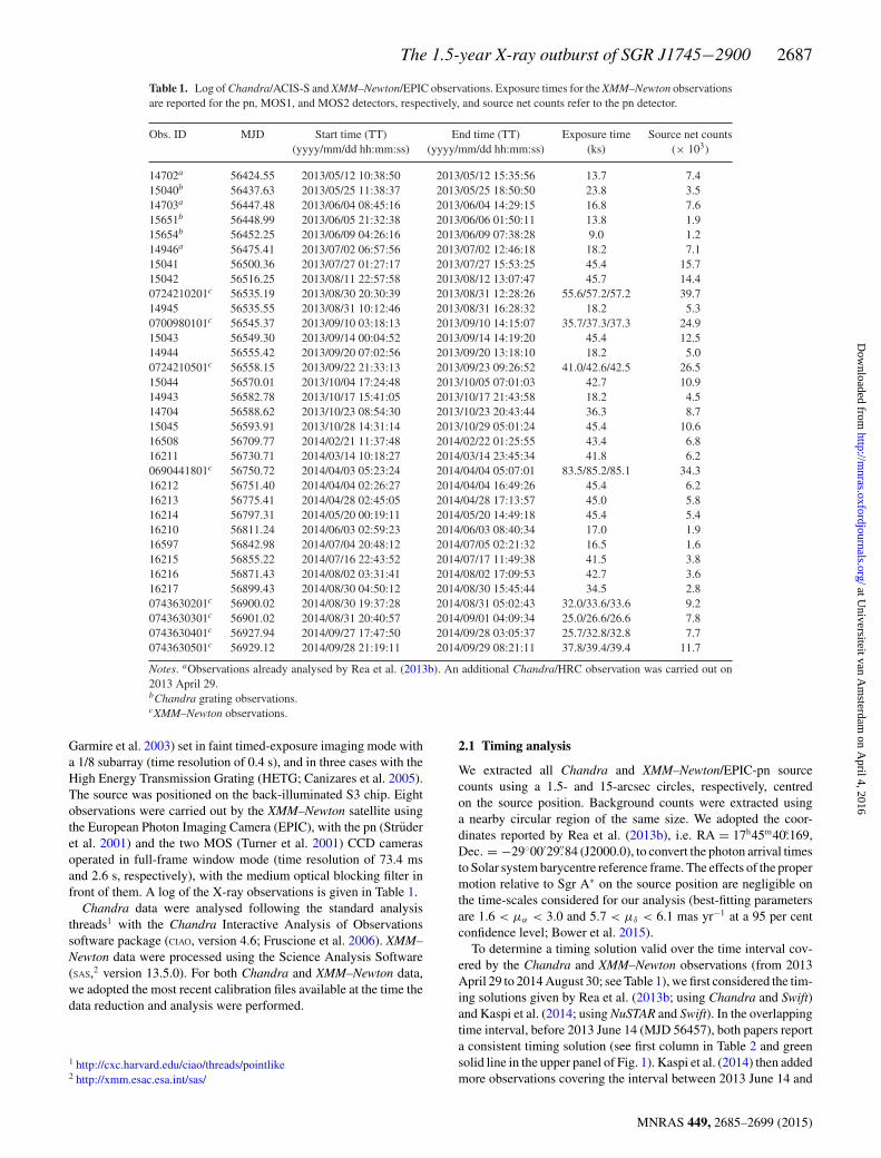
Table 1. Log of Chandra/ACIS-S and XMM–Newton/EPIC observations. Exposure times for the XMM–Newton observationsare reported for the pn, MOS1, and MOS2 detectors, respectively, and source net counts refer to the pn detector.

Obs. ID MJD Start time (TT) End time (TT) Exposure time Source net counts(yyyy/mm/dd hh:mm:ss) (yyyy/mm/dd hh:mm:ss) (ks) (× 103)

14702a 56424.55 2013/05/12 10:38:50 2013/05/12 15:35:56 13.7 7.415040b 56437.63 2013/05/25 11:38:37 2013/05/25 18:50:50 23.8 3.514703a 56447.48 2013/06/04 08:45:16 2013/06/04 14:29:15 16.8 7.615651b 56448.99 2013/06/05 21:32:38 2013/06/06 01:50:11 13.8 1.915654b 56452.25 2013/06/09 04:26:16 2013/06/09 07:38:28 9.0 1.214946a 56475.41 2013/07/02 06:57:56 2013/07/02 12:46:18 18.2 7.115041 56500.36 2013/07/27 01:27:17 2013/07/27 15:53:25 45.4 15.715042 56516.25 2013/08/11 22:57:58 2013/08/12 13:07:47 45.7 14.40724210201c 56535.19 2013/08/30 20:30:39 2013/08/31 12:28:26 55.6/57.2/57.2 39.714945 56535.55 2013/08/31 10:12:46 2013/08/31 16:28:32 18.2 5.30700980101c 56545.37 2013/09/10 03:18:13 2013/09/10 14:15:07 35.7/37.3/37.3 24.915043 56549.30 2013/09/14 00:04:52 2013/09/14 14:19:20 45.4 12.514944 56555.42 2013/09/20 07:02:56 2013/09/20 13:18:10 18.2 5.00724210501c 56558.15 2013/09/22 21:33:13 2013/09/23 09:26:52 41.0/42.6/42.5 26.515044 56570.01 2013/10/04 17:24:48 2013/10/05 07:01:03 42.7 10.914943 56582.78 2013/10/17 15:41:05 2013/10/17 21:43:58 18.2 4.514704 56588.62 2013/10/23 08:54:30 2013/10/23 20:43:44 36.3 8.715045 56593.91 2013/10/28 14:31:14 2013/10/29 05:01:24 45.4 10.616508 56709.77 2014/02/21 11:37:48 2014/02/22 01:25:55 43.4 6.816211 56730.71 2014/03/14 10:18:27 2014/03/14 23:45:34 41.8 6.20690441801c 56750.72 2014/04/03 05:23:24 2014/04/04 05:07:01 83.5/85.2/85.1 34.316212 56751.40 2014/04/04 02:26:27 2014/04/04 16:49:26 45.4 6.216213 56775.41 2014/04/28 02:45:05 2014/04/28 17:13:57 45.0 5.816214 56797.31 2014/05/20 00:19:11 2014/05/20 14:49:18 45.4 5.416210 56811.24 2014/06/03 02:59:23 2014/06/03 08:40:34 17.0 1.916597 56842.98 2014/07/04 20:48:12 2014/07/05 02:21:32 16.5 1.616215 56855.22 2014/07/16 22:43:52 2014/07/17 11:49:38 41.5 3.816216 56871.43 2014/08/02 03:31:41 2014/08/02 17:09:53 42.7 3.616217 56899.43 2014/08/30 04:50:12 2014/08/30 15:45:44 34.5 2.80743630201c 56900.02 2014/08/30 19:37:28 2014/08/31 05:02:43 32.0/33.6/33.6 9.20743630301c 56901.02 2014/08/31 20:40:57 2014/09/01 04:09:34 25.0/26.6/26.6 7.80743630401c 56927.94 2014/09/27 17:47:50 2014/09/28 03:05:37 25.7/32.8/32.8 7.70743630501c 56929.12 2014/09/28 21:19:11 2014/09/29 08:21:11 37.8/39.4/39.4 11.7

Notes. aObservations already analysed by Rea et al. (2013b). An additional Chandra/HRC observation was carried out on2013 April 29.bChandra grating observations.cXMM–Newton observations.

Garmire et al. 2003) set in faint timed-exposure imaging mode witha 1/8 subarray (time resolution of 0.4 s), and in three cases with theHigh Energy Transmission Grating (HETG; Canizares et al. 2005).The source was positioned on the back-illuminated S3 chip. Eightobservations were carried out by the XMM–Newton satellite usingthe European Photon Imaging Camera (EPIC), with the pn (Struderet al. 2001) and the two MOS (Turner et al. 2001) CCD camerasoperated in full-frame window mode (time resolution of 73.4 msand 2.6 s, respectively), with the medium optical blocking filter infront of them. A log of the X-ray observations is given in Table 1.

Chandra data were analysed following the standard analysisthreads1 with the Chandra Interactive Analysis of Observationssoftware package (CIAO, version 4.6; Fruscione et al. 2006). XMM–Newton data were processed using the Science Analysis Software(SAS,2 version 13.5.0). For both Chandra and XMM–Newton data,we adopted the most recent calibration files available at the time thedata reduction and analysis were performed.

1 http://cxc.harvard.edu/ciao/threads/pointlike2 http://xmm.esac.esa.int/sas/

2.1 Timing analysis

We extracted all Chandra and XMM–Newton/EPIC-pn sourcecounts using a 1.5- and 15-arcsec circles, respectively, centredon the source position. Background counts were extracted usinga nearby circular region of the same size. We adopted the coor-dinates reported by Rea et al. (2013b), i.e. RA = 17h45m40.s169,Dec. = −29◦00′29.′′84 (J2000.0), to convert the photon arrival timesto Solar system barycentre reference frame. The effects of the propermotion relative to Sgr A∗ on the source position are negligible onthe time-scales considered for our analysis (best-fitting parametersare 1.6 < μα < 3.0 and 5.7 < μδ < 6.1 mas yr−1 at a 95 per centconfidence level; Bower et al. 2015).

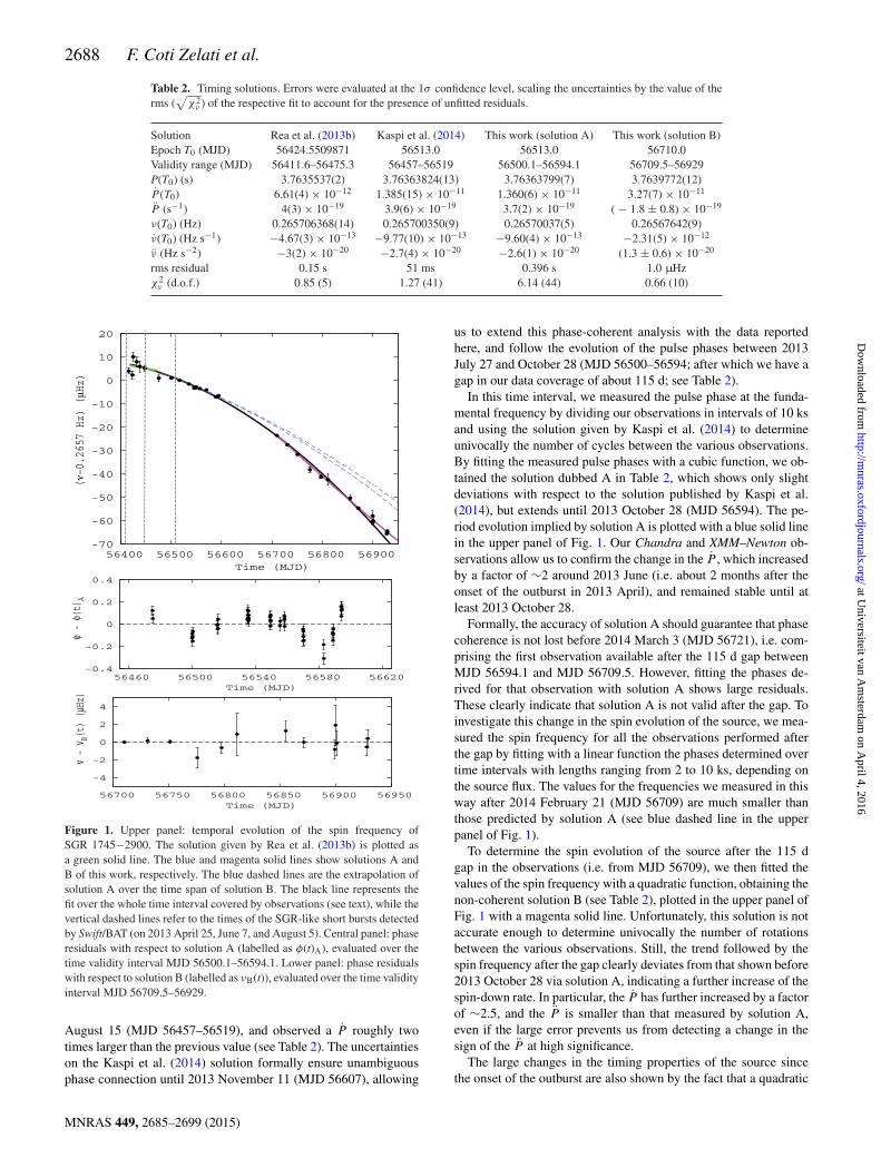
To determine a timing solution valid over the time interval cov-ered by the Chandra and XMM–Newton observations (from 2013April 29 to 2014 August 30; see Table 1), we first considered the tim-ing solutions given by Rea et al. (2013b; using Chandra and Swift)and Kaspi et al. (2014; using NuSTAR and Swift). In the overlappingtime interval, before 2013 June 14 (MJD 56457), both papers reporta consistent timing solution (see first column in Table 2 and greensolid line in the upper panel of Fig. 1). Kaspi et al. (2014) then addedmore observations covering the interval between 2013 June 14 and

MNRAS 449, 2685–2699 (2015)


msterdam

on April 4, 2016


Dow

nloaded from

http://cxc.harvard.edu/ciao/threads/pointlike

http://xmm.esac.esa.int/sas/



Table 2. Timing solutions. Errors were evaluated at the 1σ confidence level, scaling the uncertainties by the value of therms (

√χ2

ν ) of the respective fit to account for the presence of unfitted residuals.

Solution Rea et al. (2013b) Kaspi et al. (2014) This work (solution A) This work (solution B)Epoch T0 (MJD) 56424.5509871 56513.0 56513.0 56710.0Validity range (MJD) 56411.6–56475.3 56457–56519 56500.1–56594.1 56709.5–56929P(T0) (s) 3.7635537(2) 3.76363824(13) 3.76363799(7) 3.7639772(12)P (T0) 6.61(4) × 10−12 1.385(15) × 10−11 1.360(6) × 10−11 3.27(7) × 10−11

P (s−1) 4(3) × 10−19 3.9(6) × 10−19 3.7(2) × 10−19 ( − 1.8 ± 0.8) × 10−19

ν(T0) (Hz) 0.265706368(14) 0.265700350(9) 0.26570037(5) 0.26567642(9)ν(T0) (Hz s−1) −4.67(3) × 10−13 −9.77(10) × 10−13 −9.60(4) × 10−13 −2.31(5) × 10−12

ν (Hz s−2) −3(2) × 10−20 −2.7(4) × 10−20 −2.6(1) × 10−20 (1.3 ± 0.6) × 10−20

rms residual 0.15 s 51 ms 0.396 s 1.0 µHzχ2

ν (d.o.f.) 0.85 (5) 1.27 (41) 6.14 (44) 0.66 (10)

-70

-60

-50

-40

-30

-20

-10

0

10

20

56400 56500 56600 56700 56800 56900

(-0.2657 Hz) (Hz)

Time (MJD)

-0.4

-0.2

0

0.2

0.4

56460 56500 56540 56580 56620

φ -

φ (t)

A

Time (MJD)

-4

-2

0

2

4

56700 56750 56800 56850 56900 56950

ν -

ν B(t) ( μHz)

Time (MJD)

Figure 1. Upper panel: temporal evolution of the spin frequency ofSGR 1745−2900. The solution given by Rea et al. (2013b) is plotted asa green solid line. The blue and magenta solid lines show solutions A andB of this work, respectively. The blue dashed lines are the extrapolation ofsolution A over the time span of solution B. The black line represents thefit over the whole time interval covered by observations (see text), while thevertical dashed lines refer to the times of the SGR-like short bursts detectedby Swift/BAT (on 2013 April 25, June 7, and August 5). Central panel: phaseresiduals with respect to solution A (labelled as φ(t)A), evaluated over thetime validity interval MJD 56500.1–56594.1. Lower panel: phase residualswith respect to solution B (labelled as νB(t)), evaluated over the time validityinterval MJD 56709.5–56929.

August 15 (MJD 56457–56519), and observed a P roughly twotimes larger than the previous value (see Table 2). The uncertaintieson the Kaspi et al. (2014) solution formally ensure unambiguousphase connection until 2013 November 11 (MJD 56607), allowing

us to extend this phase-coherent analysis with the data reportedhere, and follow the evolution of the pulse phases between 2013July 27 and October 28 (MJD 56500–56594; after which we have agap in our data coverage of about 115 d; see Table 2).

In this time interval, we measured the pulse phase at the funda-mental frequency by dividing our observations in intervals of 10 ksand using the solution given by Kaspi et al. (2014) to determineunivocally the number of cycles between the various observations.By fitting the measured pulse phases with a cubic function, we ob-tained the solution dubbed A in Table 2, which shows only slightdeviations with respect to the solution published by Kaspi et al.(2014), but extends until 2013 October 28 (MJD 56594). The pe-riod evolution implied by solution A is plotted with a blue solid linein the upper panel of Fig. 1. Our Chandra and XMM–Newton ob-servations allow us to confirm the change in the P , which increasedby a factor of ∼2 around 2013 June (i.e. about 2 months after theonset of the outburst in 2013 April), and remained stable until atleast 2013 October 28.

Formally, the accuracy of solution A should guarantee that phasecoherence is not lost before 2014 March 3 (MJD 56721), i.e. com-prising the first observation available after the 115 d gap betweenMJD 56594.1 and MJD 56709.5. However, fitting the phases de-rived for that observation with solution A shows large residuals.These clearly indicate that solution A is not valid after the gap. Toinvestigate this change in the spin evolution of the source, we mea-sured the spin frequency for all the observations performed afterthe gap by fitting with a linear function the phases determined overtime intervals with lengths ranging from 2 to 10 ks, depending onthe source flux. The values for the frequencies we measured in thisway after 2014 February 21 (MJD 56709) are much smaller thanthose predicted by solution A (see blue dashed line in the upperpanel of Fig. 1).

To determine the spin evolution of the source after the 115 dgap in the observations (i.e. from MJD 56709), we then fitted thevalues of the spin frequency with a quadratic function, obtaining thenon-coherent solution B (see Table 2), plotted in the upper panel ofFig. 1 with a magenta solid line. Unfortunately, this solution is notaccurate enough to determine univocally the number of rotationsbetween the various observations. Still, the trend followed by thespin frequency after the gap clearly deviates from that shown before2013 October 28 via solution A, indicating a further increase of thespin-down rate. In particular, the P has further increased by a factorof ∼2.5, and the P is smaller than that measured by solution A,even if the large error prevents us from detecting a change in thesign of the P at high significance.

The large changes in the timing properties of the source sincethe onset of the outburst are also shown by the fact that a quadratic

MNRAS 449, 2685–2699 (2015)


msterdam

on April 4, 2016


Dow

nloaded from



0 0.5 1 1.5 20.3

0.4

0.5

0.6

0.7

Nor

mal

ized

inte

nsity

Phase (cycle)0 0.5 1 1.5 2

0.12

0.14

0.16

0.18

0.2

Nor

mal

ized

inte

nsity

Phase (cycle)0 0.5 1 1.5 2

0.4

0.6

Nor

mal

ized

inte

nsity

Phase (cycle)0 0.5 1 1.5 2

0.1

0.15

0.2

Nor

mal

ized

inte

nsity

Phase (cycle)0 0.5 1 1.5 2

0.1

0.15

0.2

Nor

mal

ized

inte

nsity

Phase (cycle)

0 0.5 1 1.5 2

0.2

0.3

0.4

0.5

Nor

mal

ized

inte

nsity

Phase (cycle)0 0.5 1 1.5 2

0.2

0.3

0.4

0.5

Nor

mal

ized

inte

nsity

Phase (cycle)0 0.5 1 1.5 2

0.2

0.3

0.4

Nor

mal

ized

inte

nsity

Phase (cycle)0 0.5 1 1.5 2

0.2

0.3

0.4

Nor

mal

ized

inte

nsity

Phase (cycle)0 0.5 1 1.5 2

0.2

0.3

0.4

Nor

mal

ized

inte

nsity

Phase (cycle)

0 0.5 1 1.5 2

0.2

0.3

0.4

Nor

mal

ized

inte

nsity

Phase (cycle)0 0.5 1 1.5 2

0.2

0.3

0.4

Nor

mal

ized

inte

nsity

Phase (cycle)0 0.5 1 1.5 2

0.15

0.2

0.25

0.3

0.35

Nor

mal

ized

inte

nsity

Phase (cycle)0 0.5 1 1.5 2

0.2

0.3

0.4

Nor

mal

ized

inte

nsity

Phase (cycle)0 0.5 1 1.5 2

0.2

0.3

0.4

Nor

mal

ized

inte

nsity

Phase (cycle)

0 0.5 1 1.5 2

0.1

0.15

0.2

0.25

Nor

mal

ized

inte

nsity

Phase (cycle)0 0.5 1 1.5 2

0.1

0.15

0.2

0.25

Nor

mal

ized

inte

nsity

Phase (cycle)0 0.5 1 1.5 2

0.1

0.15

0.2

Nor

mal

ized

inte

nsity

Phase (cycle)0 0.5 1 1.5 2

0.1

0.15

0.2

Nor

mal

ized

inte

nsity

Phase (cycle)0 0.5 1 1.5 2

0.1

0.15

Nor

mal

ized

inte

nsity

Phase (cycle)

0 0.5 1 1.5 2

0.1

0.15

Nor

mal

ized

inte

nsity

Phase (cycle)0 0.5 1 1.5 2

0.05

0.1

0.15

Nor

mal

ized

inte

nsity

Phase (cycle)0 0.5 1 1.5 2

0.06

0.08

0.1

0.12

0.14

Nor

mal

ized

inte

nsity

Phase (cycle)0 0.5 1 1.5 2

0.05

0.1

Nor

mal

ized

inte

nsity

Phase (cycle)0 0.5 1 1.5 2

0.05

0.1

Nor

mal

ized

inte

nsity

Phase (cycle)

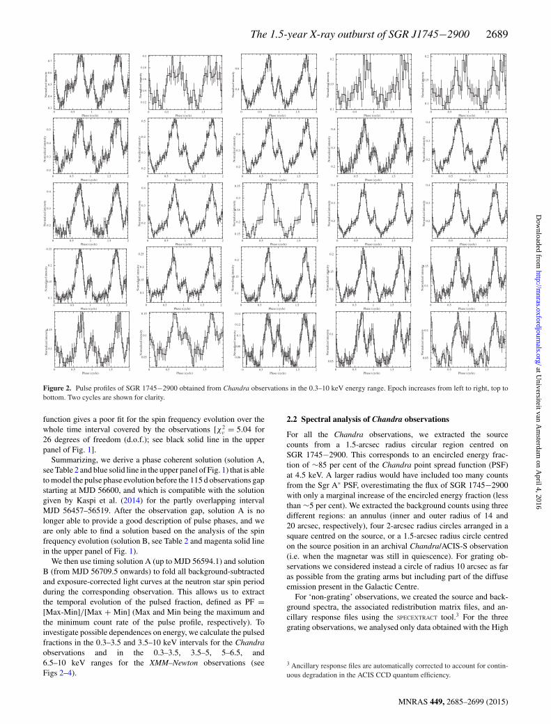
Figure 2. Pulse profiles of SGR 1745−2900 obtained from Chandra observations in the 0.3–10 keV energy range. Epoch increases from left to right, top tobottom. Two cycles are shown for clarity.

function gives a poor fit for the spin frequency evolution over thewhole time interval covered by the observations [χ2

ν = 5.04 for26 degrees of freedom (d.o.f.); see black solid line in the upperpanel of Fig. 1].

Summarizing, we derive a phase coherent solution (solution A,see Table 2 and blue solid line in the upper panel of Fig. 1) that is ableto model the pulse phase evolution before the 115 d observations gapstarting at MJD 56600, and which is compatible with the solutiongiven by Kaspi et al. (2014) for the partly overlapping intervalMJD 56457–56519. After the observation gap, solution A is nolonger able to provide a good description of pulse phases, and weare only able to find a solution based on the analysis of the spinfrequency evolution (solution B, see Table 2 and magenta solid linein the upper panel of Fig. 1).

We then use timing solution A (up to MJD 56594.1) and solutionB (from MJD 56709.5 onwards) to fold all background-subtractedand exposure-corrected light curves at the neutron star spin periodduring the corresponding observation. This allows us to extractthe temporal evolution of the pulsed fraction, defined as PF =[Max-Min]/[Max + Min] (Max and Min being the maximum andthe minimum count rate of the pulse profile, respectively). Toinvestigate possible dependences on energy, we calculate the pulsedfractions in the 0.3–3.5 and 3.5–10 keV intervals for the Chandraobservations and in the 0.3–3.5, 3.5–5, 5–6.5, and6.5–10 keV ranges for the XMM–Newton observations (seeFigs 2–4).

2.2 Spectral analysis of Chandra observations

For all the Chandra observations, we extracted the sourcecounts from a 1.5-arcsec radius circular region centred onSGR 1745−2900. This corresponds to an encircled energy frac-tion of ∼85 per cent of the Chandra point spread function (PSF)at 4.5 keV. A larger radius would have included too many countsfrom the Sgr A∗ PSF, overestimating the flux of SGR 1745−2900with only a marginal increase of the encircled energy fraction (lessthan ∼5 per cent). We extracted the background counts using threedifferent regions: an annulus (inner and outer radius of 14 and20 arcsec, respectively), four 2-arcsec radius circles arranged in asquare centred on the source, or a 1.5-arcsec radius circle centredon the source position in an archival Chandra/ACIS-S observation(i.e. when the magnetar was still in quiescence). For grating ob-servations we considered instead a circle of radius 10 arcsec as faras possible from the grating arms but including part of the diffuseemission present in the Galactic Centre.

For ‘non-grating’ observations, we created the source and back-ground spectra, the associated redistribution matrix files, and an-cillary response files using the SPECEXTRACT tool.3 For the threegrating observations, we analysed only data obtained with the High

3 Ancillary response files are automatically corrected to account for contin-uous degradation in the ACIS CCD quantum efficiency.

MNRAS 449, 2685–2699 (2015)


msterdam

on April 4, 2016


Dow

nloaded from



100 200 300 400 500

0.35

0.4

0.45

0.5

Puls

ed f

ract

ion

Time since 2013/04/24 (d)

ChandraXMM−Newton

Figure 3. Temporal evolution of the pulsed fraction (see text for our defini-tion). Uncertainties on the values were obtained by propagating the errors onthe maximum and minimum count rates. Top panel: in the 0.3–10 keV band.Central panel: in the 0.3–3.5 band for the Chandra (black triangles) andXMM–Newton (red points) observations. Bottom panel: in the 3.5–10 bandfor the Chandra observations (black) and in the 3.5–5 (blue), 5–6.5 (lightblue), and 6.5–10 keV (green) ranges for the XMM–Newton observations.

Energy Grating (0.8–8 keV). In all cases SGR 1745−2900 was off-set from the zeroth-order aim point, which was centred on the nom-inal Sgr A∗ coordinates [RA = 17h45m40.s00, Dec. = −29◦00′28.′′1(J2000.0)]. We extracted zeroth-order spectra with the TGEXTRACT

tool and generated redistribution matrices and ancillary responsefiles using MKGRMF and FULLGARF, respectively.

We grouped background-subtracted spectra to have at least 50counts per energy bin, and fitted in the 0.3–8 keV energy band

(0.8–8 keV for grating observations) with the XSPEC4 spectral fittingpackage (version 12.8.1g; Arnaud 1996), using the χ2 statistics. Thephotoelectric absorption was described through the TBABS modelwith photoionization cross-sections from Verner et al. (1996) andchemical abundances from Wilms, Allen & McCray (2000). Thesmall Chandra PSF ensures a negligible impact of the backgroundat low energies and allows us to better constrain the value of thehydrogen column density towards the source.

We estimated the impact of photon pile-up in the non-grating ob-servations by fitting all the spectra individually. Given the pile-upfraction (up to ∼30 per cent for the first observation as determinedwith WebPIMMS, version 4.7), we decided to correct for this effectusing the pile-up model of Davis (2001), as implemented in XSPEC.According to ‘The Chandra ABC Guide to Pile-up’,5 the only pa-rameters allowed to vary were the grade-migration parameter (α),and the fraction of events in the source extraction region within thecentral, piled up, portion of the PSF. Including this component inthe spectral modelling, the fits quality and the shape of the resid-uals improve substantially especially for the spectra of the first 12observations (from obs ID 14702 to 15045), when the flux is larger.We then compared our results over the three different backgroundextraction methods (see above) and found no significant differencesin the parameters, implying that our reported results do not de-pend significantly on the exact location of the selected backgroundregion.

We fitted all non-grating spectra together, adopting four differentmodels: a blackbody, a power law, the sum of two blackbodies,and a blackbody plus a power law. For all the models, we left allparameters free to vary. However, the hydrogen column density wasfound to be consistent with being constant within the errors6 amongall observations and thus was tied to be the same. We then checkedthat the inclusion of the pile-up model in the joint fits did not alterthe spectral parameters for the last 10 observations (from obs ID16508 onwards), when the flux is lower, by fitting the correspondingspectra individually without the pile-up component. The values forthe parameters are found to be consistent with being the same in allcases.

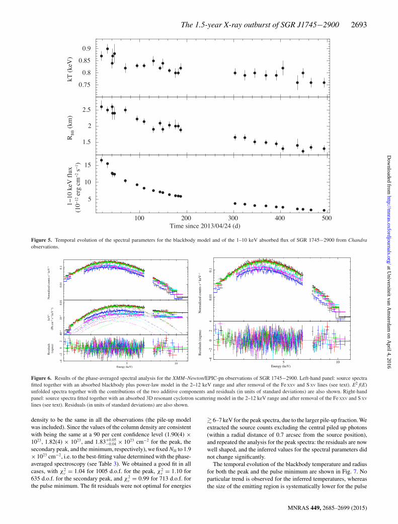
A fit with an absorbed blackbody model yields χ2ν = 1.00 for

2282 d.o.f., with a hydrogen column density NH = 1.90(2) ×1023 cm−2, temperature in the 0.76–0.90 keV range, and emittingradius in the 1.2–2.5 km interval. When an absorbed power-lawmodel is used (χ2

ν = 1.05 for 2282 d.o.f.), the photon index iswithin the range 4.2–4.9, much larger than what is usually observedfor this class of sources (see Mereghetti 2008; Rea & Esposito2011 for reviews). Moreover, a larger absorption value is obtained(NH ∼ 3 × 1023 cm−2). The large values for the photon index andthe absorption are likely not intrinsic to the source, but rather anartefact of the fitting process which tends to increase the absorp-tion to compensate for the large flux at low energies defined by thepower law. The addition of a second component to the blackbody,i.e. another blackbody or a power law, is not statistically required(χ2

ν = 1.00 for 2238 d.o.f. in both cases). We thus conclude that asingle absorbed blackbody provides the best modelling of the sourcespectrum in the 0.3–8 keV energy range (see Table 3).

Taking the absorbed blackbody as a baseline, we tried to model allthe spectra tying either the radius or the temperature to be the same

4 http://heasarc.gsfc.nasa.gov/xanadu/xspec/5 http://cxc.harvard.edu/ciao/download/doc/pile-up−abc.pdf6 Here, and in the following, uncertainties are quoted at the 90 per centconfidence level, unless otherwise noted.

MNRAS 449, 2685–2699 (2015)


msterdam

on April 4, 2016


Dow

nloaded from

http://heasarc.gsfc.nasa.gov/xanadu/xspec/

http://cxc.harvard.edu/ciao/download/doc/pile-up



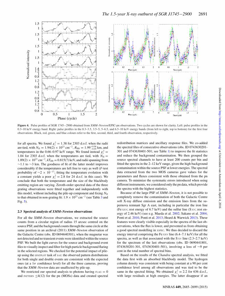
Figure 4. Pulse profiles of SGR 1745−2900 obtained from XMM–Newton/EPIC-pn observations. Two cycles are shown for clarity. Left: pulse profiles in the0.3–10 keV energy band. Right: pulse profiles in the 0.3–3.5, 3.5–5, 5–6.5, and 6.5–10 keV energy bands (from left to right, top to bottom) for the first fourobservations. Black, red, green, and blue colours refer to the first, second, third, and fourth observation, respectively.

for all spectra. We found χ2ν = 1.38 for 2303 d.o.f. when the radii

are tied, with NH = 1.94(2) × 1023 cm−2, RBB = 1.99+0.06−0.05 km, and

temperatures in the 0.66–0.97 keV range. We found instead χ2ν =

1.04 for 2303 d.o.f. when the temperatures are tied, with NH =1.89(2) × 1023 cm−2, kTBB = 0.815(7) keV, and radii spanning from∼1.1 to ∼3 km. The goodness of fit of the latter model improvesconsiderably if the temperatures are left free to vary as well (F-testprobability of ∼2 × 10−17; fitting the temperature evolution witha constant yields a poor χ2

ν = 2.8 for 24 d.o.f. in this case). Weconclude that both the temperature and the size of the blackbodyemitting region are varying. Zeroth-order spectral data of the threegrating observations were fitted together and independently withthis model, without including the pile-up component and fixing NH

to that obtained in non-grating fit: 1.9 × 1023 cm−2 (see Table 3 andFig. 5).

2.3 Spectral analysis of XMM–Newton observations

For all the XMM–Newton observations, we extracted the sourcecounts from a circular region of radius 15 arcsec centred on thesource PSF, and the background counts through the same circle at thesame position in an archival (2011) XMM–Newton observation ofthe Galactic Centre (obs. ID 0694640301), when the magnetar wasnot detected and no transient events were identified within the sourcePSF. We built the light curves for the source and background eventfiles to visually inspect and filter for high particle background flaringin the selected regions. We checked for the potential impact of pile-up using the EPATPLOT task of SAS: the observed pattern distributionsfor both single and double events are consistent with the expectedones (at a 1σ confidence level) for all the three cameras, provingthat the XMM–Newton data are unaffected by pile-up.

We restricted our spectral analysis to photons having FLAG = 0and PATTERN ≤4(12) for the pn (MOSs) data and created spectral

redistribution matrices and ancillary response files. We co-addedthe spectral files of consecutive observations (obs. ID 0743630201-301 and 0743630401-501; see Table 1) to improve the fit statisticsand reduce the background contamination. We then grouped thesource spectral channels to have at least 200 counts per bin andfitted the spectra in the 2–12 keV range, given the high backgroundcontamination within the source PSF at lower energies. The spectraldata extracted from the two MOS cameras gave values for theparameters and fluxes consistent with those obtained from the pncamera. To minimize the systematic errors introduced when usingdifferent instruments, we considered only the pn data, which providethe spectra with the highest statistics.

Because of the large PSF of XMM–Newton, it is not possible tocompletely remove the contamination of both the Galactic Centresoft X-ray diffuse emission and the emission lines from the su-pernova remnant Sgr A east, including in particular the iron line(Fe XXV; rest energy of 6.7 keV) and the sulfur line (S XV; rest en-ergy of 2.46 keV) (see e.g. Maeda et al. 2002; Sakano et al. 2004;Ponti et al. 2010, Ponti et al. 2013; Heard & Warwick 2013). Thesefeatures were clearly visible especially in the spectra of the last ob-servations, when the flux is lower, and prevented us from obtaininga good spectral modelling in XSPEC. We thus decided to discard theenergy interval comprising the Fe XXV line (6.4–7.1 keV) for all thespectra, as well as that associated with the S XV line (2.3–2.7 keV)for the spectrum of the last observations (obs. ID 0690441801,0743630201-301, 0743630401-501), involving a loss of ∼9 percent in the total number of spectral bins.

Based on the results of the Chandra spectral analysis, we fittedthe data first with an absorbed blackbody model. The hydrogencolumn density was consistent with being constant at a 90 per centconfidence level among all observations and was tied to be thesame in the spectral fitting. We obtained χ2

ν = 2.2 for 636 d.o.f.,with large residuals at high energies. The latter disappear if an

MNRAS 449, 2685–2699 (2015)


msterdam

on April 4, 2016


Dow

nloaded from



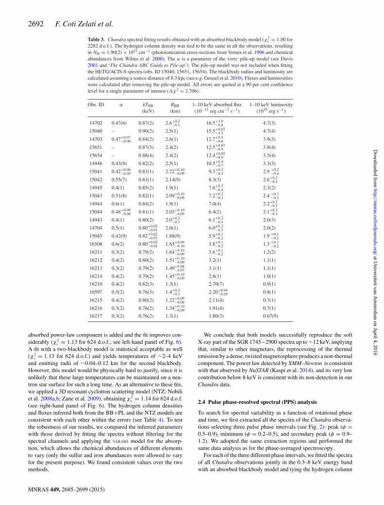
Table 3. Chandra spectral fitting results obtained with an absorbed blackbody model (χ2ν = 1.00 for

2282 d.o.f.). The hydrogen column density was tied to be the same in all the observations, resultingin NH = 1.90(2) × 1023 cm−2 (photoionization cross-sections from Verner et al. 1996 and chemicalabundances from Wilms et al. 2000). The α is a parameter of the XSPEC pile-up model (see Davis2001 and ‘The Chandra ABC Guide to Pile-up’). The pile-up model was not included when fittingthe HETG/ACIS-S spectra (obs. ID 15040, 15651, 15654). The blackbody radius and luminosity arecalculated assuming a source distance of 8.3 kpc (see e.g. Genzel et al. 2010). Fluxes and luminositieswere calculated after removing the pile-up model. All errors are quoted at a 90 per cent confidencelevel for a single parameter of interest (χ2 = 2.706).

Obs. ID α kTBB RBB 1–10 keV absorbed flux 1–10 keV luminosity(keV) (km) (10−12 erg cm−2 s−1) (1035 erg s−1)

14702 0.47(6) 0.87(2) 2.6+0.2−0.1 16.5+1.0

−0.8 4.7(3)

15040 – 0.90(2) 2.5(1) 15.5+0.03−1.3 4.7(4)

14703 0.47+0.07−0.06 0.84(2) 2.6(1) 12.7+0.5

−0.6 3.9(3)

15651 – 0.87(3) 2.4(2) 12.5+0.07−0.9 3.8(4)

15654 – 0.88(4) 2.4(2) 12.4+0.05−0.9 3.5(4)

14946 0.43(8) 0.82(2) 2.5(1) 10.5+0.4−0.7 3.3(3)

15041 0.42+0.06−0.05 0.83(1) 2.22+0.10

−0.09 9.3+0.2−0.3 2.9 +0.2

−0.4

15042 0.55(7) 0.83(1) 2.14(9) 8.3(3) 2.6+0.2−0.4

14945 0.4(1) 0.85(2) 1.9(1) 7.6+0.3−0.4 2.3(2)

15043 0.51(8) 0.82(1) 2.09+0.10−0.09 7.2+0.2

−0.3 2.4 +0.2−0.3

14944 0.6(1) 0.84(2) 1.9(1) 7.0(4) 2.2+0.2−0.3

15044 0.48+0.09−0.08 0.81(1) 2.03+0.10

−0.09 6.4(2) 2.1+0.2−0.3

14943 0.4(1) 0.80(2) 2.0+0.2−0.1 6.1+0.2

−0.4 2.0(3)

14704 0.5(1) 0.80+0.02−0.01 2.0(1) 6.0+0.2

−0.3 2.0(2)

15045 0.42(9) 0.82+0.02−0.01 1.88(9) 5.9+0.1

−0.2 1.9 +0.1−0.2

16508 0.6(2) 0.80+0.02−0.01 1.65+0.09

−0.10 3.8+0.1−0.2 1.3 +0.1

−0.2

16211 0.3(2) 0.79(2) 1.64+0.10−0.09 3.6+0.1

−0.2 1.2(2)

16212 0.4(2) 0.80(2) 1.51+0.10−0.09 3.2(1) 1.1(1)

16213 0.3(2) 0.79(2) 1.49+0.08−0.07 3.1(1) 1.1(1)

16214 0.4(2) 0.79(2) 1.45+0.10−0.09 2.8(1) 1.0(1)

16210 0.4(2) 0.82(3) 1.3(1) 2.70(7) 0.9(1)

16597 0.5(2) 0.76(3) 1.4+0.2−0.1 2.20+0.04

−0.05 0.8(1)

16215 0.4(2) 0.80(2) 1.22+0.09−0.08 2.11(4) 0.7(1)

16216 0.3(2) 0.76(2) 1.34+0.10−0.09 1.91(4) 0.7(1)

16217 0.3(2) 0.76(2) 1.3(1) 1.80(3) 0.67(9)

absorbed power-law component is added and the fit improves con-siderably (χ2

ν = 1.13 for 624 d.o.f.; see left-hand panel of Fig. 6).A fit with a two-blackbody model is statistical acceptable as well(χ2

ν = 1.13 for 624 d.o.f.) and yields temperatures of ∼2–4 keVand emitting radii of ∼0.04–0.12 km for the second blackbody.However, this model would be physically hard to justify, since it isunlikely that these large temperatures can be maintained on a neu-tron star surface for such a long time. As an alternative to these fits,we applied a 3D resonant cyclotron scattering model (NTZ; Nobiliet al. 2008a,b; Zane et al. 2009), obtaining χ2

ν = 1.14 for 624 d.o.f.(see right-hand panel of Fig. 6). The hydrogen column densitiesand fluxes inferred both from the BB+PL and the NTZ models areconsistent with each other within the errors (see Table 4). To testthe robustness of our results, we compared the inferred parameterswith those derived by fitting the spectra without filtering for thespectral channels and applying the VARABS model for the absorp-tion, which allows the chemical abundances of different elementsto vary (only the sulfur and iron abundances were allowed to varyfor the present purpose). We found consistent values over the twomethods.

We conclude that both models successfully reproduce the softX-ray part of the SGR 1745−2900 spectra up to ∼12 keV, implyingthat, similar to other magnetars, the reprocessing of the thermalemission by a dense, twisted magnetosphere produces a non-thermalcomponent. The power law detected by XMM–Newton is consistentwith that observed by NuSTAR (Kaspi et al. 2014), and its very lowcontribution below 8 keV is consistent with its non-detection in ourChandra data.

2.4 Pulse phase-resolved spectral (PPS) analysis

To search for spectral variability as a function of rotational phaseand time, we first extracted all the spectra of the Chandra observa-tions selecting three pulse phase intervals (see Fig. 2): peak (φ =0.5–0.9), minimum (φ = 0.2–0.5), and secondary peak (φ = 0.9–1.2). We adopted the same extraction regions and performed thesame data analysis as for the phase-averaged spectroscopy.

For each of the three different phase intervals, we fitted the spectraof all Chandra observations jointly in the 0.3–8 keV energy bandwith an absorbed blackbody model and tying the hydrogen column

MNRAS 449, 2685–2699 (2015)


msterdam

on April 4, 2016


Dow

nloaded from



0.75

0.8

0.85

0.9

kT (

keV

)

1.5

2

2.5

RB

B (

km)

100 200 300 400 500

5

10

15

(10−

12 e

rg c

m−

2 s−

1 )1 −

10 k

eV f

lux


Figure 5. Temporal evolution of the spectral parameters for the blackbody model and of the 1–10 keV absorbed flux of SGR 1745−2900 from Chandraobservations.

0.01

0.1

Nor

mal

ized

cou

nts

s−1 k

eV−

1

10−

410

−3

0.01

keV

2

(Ph

cm−

2 s−

1 keV

−1 )

105−4

−2

02

4

Res

idua

ls(s

igm

a)

Energy (keV)

0.01

0.1

Nor

mal

ized

cou

nts

s−1 k

eV−

1

105−4

−2

02

4

Res

idua

ls (

sigm

a)

Energy (keV)

Figure 6. Results of the phase-averaged spectral analysis for the XMM–Newton/EPIC-pn observations of SGR 1745−2900. Left-hand panel: source spectrafitted together with an absorbed blackbody plus power-law model in the 2–12 keV range and after removal of the Fe XXV and S XV lines (see text). E2 f(E)unfolded spectra together with the contributions of the two additive components and residuals (in units of standard deviations) are also shown. Right-handpanel: source spectra fitted together with an absorbed 3D resonant cyclotron scattering model in the 2–12 keV range and after removal of the Fe XXV and S XV

lines (see text). Residuals (in units of standard deviations) are also shown.

density to be the same in all the observations (the pile-up modelwas included). Since the values of the column density are consistentwith being the same at a 90 per cent confidence level (1.90(4) ×1023, 1.82(4) × 1023, and 1.83+0.05

−0.04 × 1023 cm−2 for the peak, thesecondary peak, and the minimum, respectively), we fixed NH to 1.9× 1023 cm−2, i.e. to the best-fitting value determined with the phase-averaged spectroscopy (see Table 3). We obtained a good fit in allcases, with χ2

ν = 1.04 for 1005 d.o.f. for the peak, χ2ν = 1.10 for

635 d.o.f. for the secondary peak, and χ2ν = 0.99 for 713 d.o.f. for

the pulse minimum. The fit residuals were not optimal for energies

� 6–7 keV for the peak spectra, due to the larger pile-up fraction. Weextracted the source counts excluding the central piled up photons(within a radial distance of 0.7 arcsec from the source position),and repeated the analysis for the peak spectra: the residuals are nowwell shaped, and the inferred values for the spectral parameters didnot change significantly.

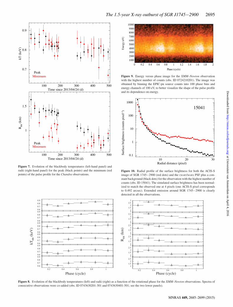
The temporal evolution of the blackbody temperature and radiusfor both the peak and the pulse minimum are shown in Fig. 7. Noparticular trend is observed for the inferred temperatures, whereasthe size of the emitting region is systematically lower for the pulse

MNRAS 449, 2685–2699 (2015)


msterdam

on April 4, 2016


Dow

nloaded from



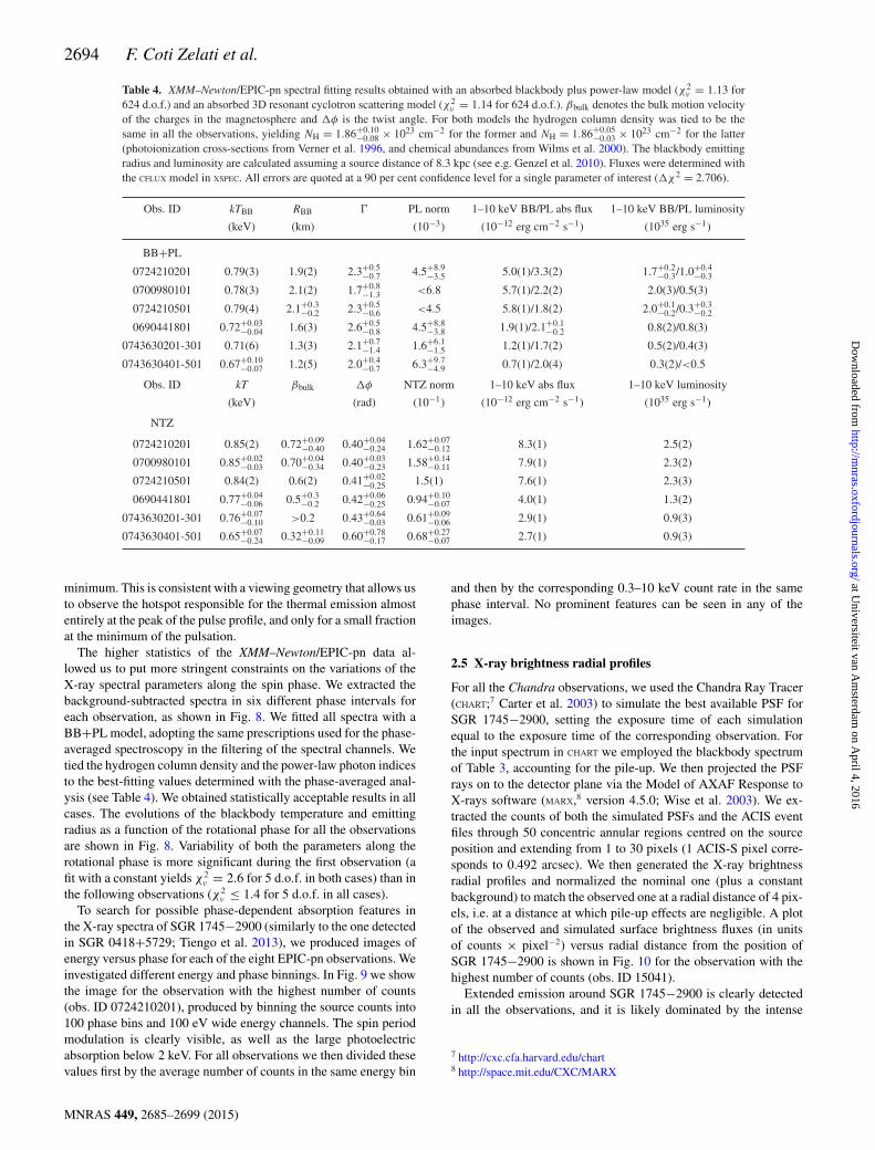
Table 4. XMM–Newton/EPIC-pn spectral fitting results obtained with an absorbed blackbody plus power-law model (χ2ν = 1.13 for

624 d.o.f.) and an absorbed 3D resonant cyclotron scattering model (χ2ν = 1.14 for 624 d.o.f.). βbulk denotes the bulk motion velocity

of the charges in the magnetosphere and φ is the twist angle. For both models the hydrogen column density was tied to be thesame in all the observations, yielding NH = 1.86+0.10

−0.08 × 1023 cm−2 for the former and NH = 1.86+0.05−0.03 × 1023 cm−2 for the latter

(photoionization cross-sections from Verner et al. 1996, and chemical abundances from Wilms et al. 2000). The blackbody emittingradius and luminosity are calculated assuming a source distance of 8.3 kpc (see e.g. Genzel et al. 2010). Fluxes were determined withthe CFLUX model in XSPEC. All errors are quoted at a 90 per cent confidence level for a single parameter of interest (χ2 = 2.706).

Obs. ID kTBB RBB � PL norm 1–10 keV BB/PL abs flux 1–10 keV BB/PL luminosity

(keV) (km) (10−3) (10−12 erg cm−2 s−1) (1035 erg s−1)

BB+PL

0724210201 0.79(3) 1.9(2) 2.3+0.5−0.7 4.5+8.9

−3.5 5.0(1)/3.3(2) 1.7+0.2−0.3/1.0+0.4

−0.3

0700980101 0.78(3) 2.1(2) 1.7+0.8−1.3 <6.8 5.7(1)/2.2(2) 2.0(3)/0.5(3)

0724210501 0.79(4) 2.1+0.3−0.2 2.3+0.5

−0.6 <4.5 5.8(1)/1.8(2) 2.0+0.1−0.2/0.3+0.3

−0.2

0690441801 0.72+0.03−0.04 1.6(3) 2.6+0.5

−0.8 4.5+8.8−3.8 1.9(1)/2.1+0.1

−0.2 0.8(2)/0.8(3)

0743630201-301 0.71(6) 1.3(3) 2.1+0.7−1.4 1.6+6.1

−1.5 1.2(1)/1.7(2) 0.5(2)/0.4(3)

0743630401-501 0.67+0.10−0.07 1.2(5) 2.0+0.4

−0.7 6.3+9.7−4.9 0.7(1)/2.0(4) 0.3(2)/<0.5

Obs. ID kT βbulk φ NTZ norm 1–10 keV abs flux 1–10 keV luminosity

(keV) (rad) (10−1) (10−12 erg cm−2 s−1) (1035 erg s−1)

NTZ

0724210201 0.85(2) 0.72+0.09−0.40 0.40+0.04

−0.24 1.62+0.07−0.12 8.3(1) 2.5(2)

0700980101 0.85+0.02−0.03 0.70+0.04

−0.34 0.40+0.03−0.23 1.58+0.14

−0.11 7.9(1) 2.3(2)

0724210501 0.84(2) 0.6(2) 0.41+0.02−0.25 1.5(1) 7.6(1) 2.3(3)

0690441801 0.77+0.04−0.06 0.5+0.3

−0.2 0.42+0.06−0.25 0.94+0.10

−0.07 4.0(1) 1.3(2)

0743630201-301 0.76+0.07−0.10 >0.2 0.43+0.64

−0.03 0.61+0.09−0.06 2.9(1) 0.9(3)

0743630401-501 0.65+0.07−0.24 0.32+0.11

−0.09 0.60+0.78−0.17 0.68+0.27

−0.07 2.7(1) 0.9(3)

minimum. This is consistent with a viewing geometry that allows usto observe the hotspot responsible for the thermal emission almostentirely at the peak of the pulse profile, and only for a small fractionat the minimum of the pulsation.

The higher statistics of the XMM–Newton/EPIC-pn data al-lowed us to put more stringent constraints on the variations of theX-ray spectral parameters along the spin phase. We extracted thebackground-subtracted spectra in six different phase intervals foreach observation, as shown in Fig. 8. We fitted all spectra with aBB+PL model, adopting the same prescriptions used for the phase-averaged spectroscopy in the filtering of the spectral channels. Wetied the hydrogen column density and the power-law photon indicesto the best-fitting values determined with the phase-averaged anal-ysis (see Table 4). We obtained statistically acceptable results in allcases. The evolutions of the blackbody temperature and emittingradius as a function of the rotational phase for all the observationsare shown in Fig. 8. Variability of both the parameters along therotational phase is more significant during the first observation (afit with a constant yields χ2

ν = 2.6 for 5 d.o.f. in both cases) than inthe following observations (χ2

ν ≤ 1.4 for 5 d.o.f. in all cases).To search for possible phase-dependent absorption features in

the X-ray spectra of SGR 1745−2900 (similarly to the one detectedin SGR 0418+5729; Tiengo et al. 2013), we produced images ofenergy versus phase for each of the eight EPIC-pn observations. Weinvestigated different energy and phase binnings. In Fig. 9 we showthe image for the observation with the highest number of counts(obs. ID 0724210201), produced by binning the source counts into100 phase bins and 100 eV wide energy channels. The spin periodmodulation is clearly visible, as well as the large photoelectricabsorption below 2 keV. For all observations we then divided thesevalues first by the average number of counts in the same energy bin

and then by the corresponding 0.3–10 keV count rate in the samephase interval. No prominent features can be seen in any of theimages.

2.5 X-ray brightness radial profiles

For all the Chandra observations, we used the Chandra Ray Tracer(CHART;7 Carter et al. 2003) to simulate the best available PSF forSGR 1745−2900, setting the exposure time of each simulationequal to the exposure time of the corresponding observation. Forthe input spectrum in CHART we employed the blackbody spectrumof Table 3, accounting for the pile-up. We then projected the PSFrays on to the detector plane via the Model of AXAF Response toX-rays software (MARX,8 version 4.5.0; Wise et al. 2003). We ex-tracted the counts of both the simulated PSFs and the ACIS eventfiles through 50 concentric annular regions centred on the sourceposition and extending from 1 to 30 pixels (1 ACIS-S pixel corre-sponds to 0.492 arcsec). We then generated the X-ray brightnessradial profiles and normalized the nominal one (plus a constantbackground) to match the observed one at a radial distance of 4 pix-els, i.e. at a distance at which pile-up effects are negligible. A plotof the observed and simulated surface brightness fluxes (in unitsof counts × pixel−2) versus radial distance from the position ofSGR 1745−2900 is shown in Fig. 10 for the observation with thehighest number of counts (obs. ID 15041).

Extended emission around SGR 1745−2900 is clearly detectedin all the observations, and it is likely dominated by the intense

7 http://cxc.cfa.harvard.edu/chart8 http://space.mit.edu/CXC/MARX

MNRAS 449, 2685–2699 (2015)


msterdam

on April 4, 2016


Dow

nloaded from

http://cxc.cfa.harvard.edu/chart

http://space.mit.edu/CXC/MARX



100 200 300 400 500

0.7

0.8

0.9

kT (

keV

)


PeakMinimum

100 200 300 400 500

1

1.5

RB

B (

km)


PeakMinimum

Figure 7. Evolution of the blackbody temperatures (left-hand panel) andradii (right-hand panel) for the peak (black points) and the minimum (redpoints) of the pulse profile for the Chandra observations.

Figure 9. Energy versus phase image for the XMM–Newton observationwith the highest number of counts (obs. ID 0724210201). The image wasobtained by binning the EPIC-pn source counts into 100 phase bins andenergy channels of 100 eV, to better visualize the shape of the pulse profileand its dependence on energy.

10 20 300.1

1

10

100

1000

Surf

ace

brig

htne

ss (

coun

ts p

ixel

−2 )

Radial distance (pixel)

15041

Figure 10. Radial profile of the surface brightness for both the ACIS-Simage of SGR 1745−2900 (red dots) and the CHART/MARX PSF plus a con-stant background (black dots) for the observation with the highest number ofcounts (obs. ID 15041). The simulated surface brightness has been normal-ized to match the observed one at 4 pixels (one ACIS-S pixel correspondsto 0.492 arcsec). Extended emission around SGR 1745−2900 is clearlydetected in all the observations.

0.6

0.7

0.8

0.9

0.6

0.7

0.8

0.9

0.6

0.7

0.8

0.9

0.6

0.7

0.8

0.9

0.6

0.7

0.8

0.9

0.2 0.4 0.6 0.8 1

0.6

0.7

0.8

0.9

kTB

B (

keV

)

Phase (cycle)

11.5

22.5

3

11.5

22.5

3

11.5

22.5

3

11.5

22.5

3

11.5

22.5

3

0.2 0.4 0.6 0.8 1

11.5

22.5

3

RB

B (

km)

Phase (cycle)

Figure 8. Evolution of the blackbody temperatures (left) and radii (right) as a function of the rotational phase for the XMM–Newton observations. Spectra ofconsecutive observations were co-added (obs. ID 0743630201-301 and 0743630401-501; see the two lower panels).

MNRAS 449, 2685–2699 (2015)


msterdam

on April 4, 2016


Dow

nloaded from



0.1 1 10 100

1

10

100

Flux

(10

−12

erg

cm

−2 s

−1 )

Time (days from burst activation)

SGR 1627−41 (2008)

CXOU J164710−455216 (2006)

SGR 0501+4516 (2008)1E 1547−5408 (2009)

SGR 0418+5729 (2009)

1E 1547−5408 (2008)

SGR 1833−0832 (2010)

Swift 1834−0846 (2011)

Swift 1822−1606 (2011)

SGR J1745−2900 (2013)

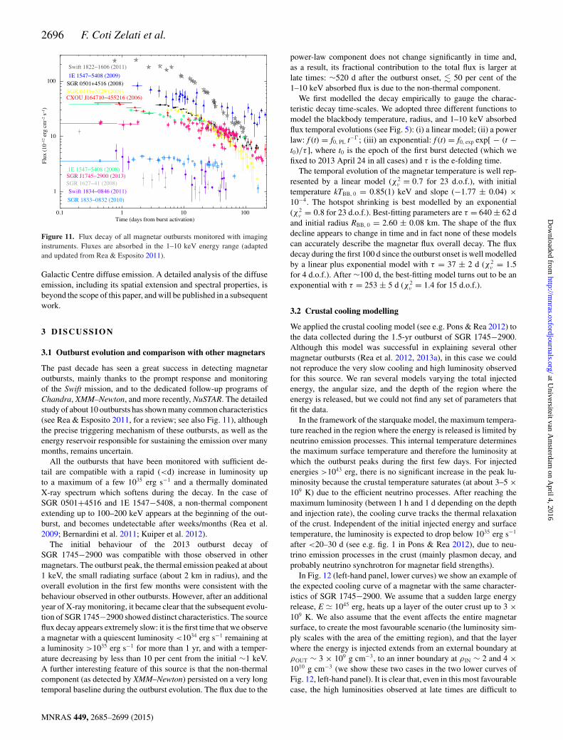
Figure 11. Flux decay of all magnetar outbursts monitored with imaginginstruments. Fluxes are absorbed in the 1–10 keV energy range (adaptedand updated from Rea & Esposito 2011).

Galactic Centre diffuse emission. A detailed analysis of the diffuseemission, including its spatial extension and spectral properties, isbeyond the scope of this paper, and will be published in a subsequentwork.

3 D ISCUSSION

3.1 Outburst evolution and comparison with other magnetars

The past decade has seen a great success in detecting magnetaroutbursts, mainly thanks to the prompt response and monitoringof the Swift mission, and to the dedicated follow-up programs ofChandra, XMM–Newton, and more recently, NuSTAR. The detailedstudy of about 10 outbursts has shown many common characteristics(see Rea & Esposito 2011, for a review; see also Fig. 11), althoughthe precise triggering mechanism of these outbursts, as well as theenergy reservoir responsible for sustaining the emission over manymonths, remains uncertain.

All the outbursts that have been monitored with sufficient de-tail are compatible with a rapid (<d) increase in luminosity upto a maximum of a few 1035 erg s−1 and a thermally dominatedX-ray spectrum which softens during the decay. In the case ofSGR 0501+4516 and 1E 1547−5408, a non-thermal componentextending up to 100–200 keV appears at the beginning of the out-burst, and becomes undetectable after weeks/months (Rea et al.2009; Bernardini et al. 2011; Kuiper et al. 2012).

The initial behaviour of the 2013 outburst decay ofSGR 1745−2900 was compatible with those observed in othermagnetars. The outburst peak, the thermal emission peaked at about1 keV, the small radiating surface (about 2 km in radius), and theoverall evolution in the first few months were consistent with thebehaviour observed in other outbursts. However, after an additionalyear of X-ray monitoring, it became clear that the subsequent evolu-tion of SGR 1745−2900 showed distinct characteristics. The sourceflux decay appears extremely slow: it is the first time that we observea magnetar with a quiescent luminosity <1034 erg s−1 remaining ata luminosity >1035 erg s−1 for more than 1 yr, and with a temper-ature decreasing by less than 10 per cent from the initial ∼1 keV.A further interesting feature of this source is that the non-thermalcomponent (as detected by XMM–Newton) persisted on a very longtemporal baseline during the outburst evolution. The flux due to the

power-law component does not change significantly in time and,as a result, its fractional contribution to the total flux is larger atlate times: ∼520 d after the outburst onset, � 50 per cent of the1–10 keV absorbed flux is due to the non-thermal component.

We first modelled the decay empirically to gauge the charac-teristic decay time-scales. We adopted three different functions tomodel the blackbody temperature, radius, and 1–10 keV absorbedflux temporal evolutions (see Fig. 5): (i) a linear model; (ii) a powerlaw: f (t) = f0, PL t−�; (iii) an exponential: f (t) = f0, exp exp[ − (t −t0)/τ ], where t0 is the epoch of the first burst detected (which wefixed to 2013 April 24 in all cases) and τ is the e-folding time.

The temporal evolution of the magnetar temperature is well rep-resented by a linear model (χ2

ν = 0.7 for 23 d.o.f.), with initialtemperature kTBB, 0 = 0.85(1) keV and slope (−1.77 ± 0.04) ×10−4. The hotspot shrinking is best modelled by an exponential(χ2

ν = 0.8 for 23 d.o.f.). Best-fitting parameters are τ = 640 ± 62 dand initial radius RBB, 0 = 2.60 ± 0.08 km. The shape of the fluxdecline appears to change in time and in fact none of these modelscan accurately describe the magnetar flux overall decay. The fluxdecay during the first 100 d since the outburst onset is well modelledby a linear plus exponential model with τ = 37 ± 2 d (χ2

ν = 1.5for 4 d.o.f.). After ∼100 d, the best-fitting model turns out to be anexponential with τ = 253 ± 5 d (χ2

ν = 1.4 for 15 d.o.f.).

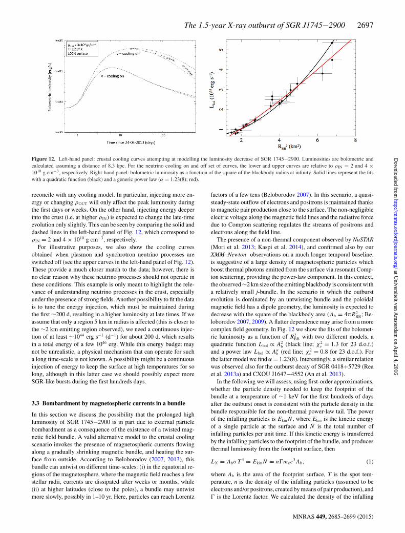
3.2 Crustal cooling modelling

We applied the crustal cooling model (see e.g. Pons & Rea 2012) tothe data collected during the 1.5-yr outburst of SGR 1745−2900.Although this model was successful in explaining several othermagnetar outbursts (Rea et al. 2012, 2013a), in this case we couldnot reproduce the very slow cooling and high luminosity observedfor this source. We ran several models varying the total injectedenergy, the angular size, and the depth of the region where theenergy is released, but we could not find any set of parameters thatfit the data.

In the framework of the starquake model, the maximum tempera-ture reached in the region where the energy is released is limited byneutrino emission processes. This internal temperature determinesthe maximum surface temperature and therefore the luminosity atwhich the outburst peaks during the first few days. For injectedenergies >1043 erg, there is no significant increase in the peak lu-minosity because the crustal temperature saturates (at about 3–5 ×109 K) due to the efficient neutrino processes. After reaching themaximum luminosity (between 1 h and 1 d depending on the depthand injection rate), the cooling curve tracks the thermal relaxationof the crust. Independent of the initial injected energy and surfacetemperature, the luminosity is expected to drop below 1035 erg s−1

after <20–30 d (see e.g. fig. 1 in Pons & Rea 2012), due to neu-trino emission processes in the crust (mainly plasmon decay, andprobably neutrino synchrotron for magnetar field strengths).

In Fig. 12 (left-hand panel, lower curves) we show an example ofthe expected cooling curve of a magnetar with the same character-istics of SGR 1745−2900. We assume that a sudden large energyrelease, E � 1045 erg, heats up a layer of the outer crust up to 3 ×109 K. We also assume that the event affects the entire magnetarsurface, to create the most favourable scenario (the luminosity sim-ply scales with the area of the emitting region), and that the layerwhere the energy is injected extends from an external boundary atρOUT ∼ 3 × 109 g cm−3, to an inner boundary at ρIN ∼ 2 and 4 ×1010 g cm−3 (we show these two cases in the two lower curves ofFig. 12, left-hand panel). It is clear that, even in this most favourablecase, the high luminosities observed at late times are difficult to

MNRAS 449, 2685–2699 (2015)


msterdam

on April 4, 2016


Dow

nloaded from



Figure 12. Left-hand panel: crustal cooling curves attempting at modelling the luminosity decrease of SGR 1745−2900. Luminosities are bolometric andcalculated assuming a distance of 8.3 kpc. For the neutrino cooling on and off set of curves, the lower and upper curves are relative to ρIN = 2 and 4 ×1010 g cm−3, respectively. Right-hand panel: bolometric luminosity as a function of the square of the blackbody radius at infinity. Solid lines represent the fitswith a quadratic function (black) and a generic power law (α = 1.23(8); red).

reconcile with any cooling model. In particular, injecting more en-ergy or changing ρOUT will only affect the peak luminosity duringthe first days or weeks. On the other hand, injecting energy deeperinto the crust (i.e. at higher ρIN) is expected to change the late-timeevolution only slightly. This can be seen by comparing the solid anddashed lines in the left-hand panel of Fig. 12, which correspond toρIN = 2 and 4 × 1010 g cm−3, respectively.

For illustrative purposes, we also show the cooling curvesobtained when plasmon and synchrotron neutrino processes areswitched off (see the upper curves in the left-hand panel of Fig. 12).These provide a much closer match to the data; however, there isno clear reason why these neutrino processes should not operate inthese conditions. This example is only meant to highlight the rele-vance of understanding neutrino processes in the crust, especiallyunder the presence of strong fields. Another possibility to fit the datais to tune the energy injection, which must be maintained duringthe first ∼200 d, resulting in a higher luminosity at late times. If weassume that only a region 5 km in radius is affected (this is closer tothe ∼2 km emitting region observed), we need a continuous injec-tion of at least ∼1044 erg s−1 (d−1) for about 200 d, which resultsin a total energy of a few 1046 erg. While this energy budget maynot be unrealistic, a physical mechanism that can operate for sucha long time-scale is not known. A possibility might be a continuousinjection of energy to keep the surface at high temperatures for solong, although in this latter case we should possibly expect moreSGR-like bursts during the first hundreds days.

3.3 Bombardment by magnetospheric currents in a bundle

In this section we discuss the possibility that the prolonged highluminosity of SGR 1745−2900 is in part due to external particlebombardment as a consequence of the existence of a twisted mag-netic field bundle. A valid alternative model to the crustal coolingscenario invokes the presence of magnetospheric currents flowingalong a gradually shrinking magnetic bundle, and heating the sur-face from outside. According to Beloborodov (2007, 2013), thisbundle can untwist on different time-scales: (i) in the equatorial re-gions of the magnetosphere, where the magnetic field reaches a fewstellar radii, currents are dissipated after weeks or months, while(ii) at higher latitudes (close to the poles), a bundle may untwistmore slowly, possibly in 1–10 yr. Here, particles can reach Lorentz

factors of a few tens (Beloborodov 2007). In this scenario, a quasi-steady-state outflow of electrons and positrons is maintained thanksto magnetic pair production close to the surface. The non-negligibleelectric voltage along the magnetic field lines and the radiative forcedue to Compton scattering regulates the streams of positrons andelectrons along the field line.

The presence of a non-thermal component observed by NuSTAR(Mori et al. 2013; Kaspi et al. 2014), and confirmed also by ourXMM–Newton observations on a much longer temporal baseline,is suggestive of a large density of magnetospheric particles whichboost thermal photons emitted from the surface via resonant Comp-ton scattering, providing the power-law component. In this context,the observed ∼2 km size of the emitting blackbody is consistent witha relatively small j-bundle. In the scenario in which the outburstevolution is dominated by an untwisting bundle and the poloidalmagnetic field has a dipole geometry, the luminosity is expected todecrease with the square of the blackbody area (Ab = 4πR2

BB; Be-loborodov 2007, 2009). A flatter dependence may arise from a morecomplex field geometry. In Fig. 12 we show the fits of the bolomet-ric luminosity as a function of R2

BB with two different models, aquadratic function Lbol ∝ A2

b (black line; χ2ν = 1.3 for 23 d.o.f.)

and a power law Lbol ∝ Aαb (red line; χ2

ν = 0.8 for 23 d.o.f.). Forthe latter model we find α = 1.23(8). Interestingly, a similar relationwas observed also for the outburst decay of SGR 0418+5729 (Reaet al. 2013a) and CXOU J1647−4552 (An et al. 2013).

In the following we will assess, using first-order approximations,whether the particle density needed to keep the footprint of thebundle at a temperature of ∼1 keV for the first hundreds of daysafter the outburst onset is consistent with the particle density in thebundle responsible for the non-thermal power-law tail. The powerof the infalling particles is EkinN , where Ekin is the kinetic energyof a single particle at the surface and N is the total number ofinfalling particles per unit time. If this kinetic energy is transferredby the infalling particles to the footprint of the bundle, and producesthermal luminosity from the footprint surface, then

LX = AbσT 4 = EkinN = n�mec3Ab, (1)

where Ab is the area of the footprint surface, T is the spot tem-perature, n is the density of the infalling particles (assumed to beelectrons and/or positrons, created by means of pair production), and� is the Lorentz factor. We calculated the density of the infalling

MNRAS 449, 2685–2699 (2015)


msterdam

on April 4, 2016


Dow

nloaded from



particles by considering the kinetic energy they need to heat thebase of the bundle spot. For a given temperature, one can estimaten as

nbomb = σT 4

me�c3∼ 4.2 × 1022 [kT /(1 keV)]4

�cm−3. (2)

On the other hand, we can estimate the density of the particlesresponsible for the resonant Compton scattering which producesthe X-ray tail as

nrcs � JBMve

� MB

4πβer∼ 1.7 × 1016 MB14

β

(r

R∗

)−1

cm−3,

(3)

where JB = (c/4π)∇ × B is the conduction current, B is the localmagnetic field, and r is the length-scale over which B varies (R∗ ∼106 cm is the star radius). In the magnetosphere of a magnetar thereal current is always very close to JB and it is mostly conducted bye± pairs (Beloborodov 2007). The abundance of pairs is accountedfor by the multiplicity factorMwhich is the ratio between the actualcharge density (including pairs) and the minimum density neededto sustain JB; the latter corresponds to a charge-separated flow inwhich the current is carried only by electrons (and ions). If thesame charge population is responsible for both resonant Comptonscattering and surface heating, the densities given by equations (2)and (3) should be equal. This implies

B14

(r

R∗

)−1

M� = 2.5 × 106

(kT

1 keV

)4

. (4)

According to Beloborodov (2013), both the Lorentz factor and thepair multiplicity change along the magnetic field lines, with typicalvalues ofM ∼ 100 (i.e. efficient pair creation), � ∼ 10 in the largestmagnetic field loops, and M ∼ 1 (i.e. charge-separated plasma),� ∼ 1 in the inner part of the magnetosphere. The previous equalitycannot be satisfied for a typical temperature of ∼0.8–1 keV, unlessthe magnetic field changes over an exceedingly small length-scale, afew metres at most. It appears, therefore, very unlikely that a singleflow can explain both surface heating and resonant up-scattering.

4 C O N C L U S I O N S

The spectacular angular resolution of Chandra and the large effec-tive area of XMM–Newton, together with an intense monitoring ofthe Galactic Centre region, has allowed us to collect an unprece-dented data set covering the outburst of SGR 1745−2900, with verylittle background contamination (which can be very severe in thisregion of the Milky Way).

The analysis of the evolution of the spin period allowed us tofind three different timing solutions between 2013 April 29 and2014 August 30, which show that the source period derivative haschanged at least twice, from 6.6 × 10−12 s s−1 in 2013 April atthe outburst onset, to 3.3 × 10−11 s s−1 in 2014 August. While thefirst P change could be related with the occurrence of an SGR-like burst (Kaspi et al. 2014), no burst has been detected from thesource close in time to the second P variation (although we cannotexclude it was missed by current instruments). This further changein the rotational evolution of the source might be related with thetiming anomaly observed in the radio band around the end of 2013(Lynch et al. 2015), unfortunately during our observing gap.

The 0.3–8 keV source spectrum is perfectly modelled by a sin-gle blackbody with temperature cooling from ∼0.9 to 0.75 keVin about 1.5 yr. A faint non-thermal component is observed withXMM–Newton. It dominates the flux at energies >8 keV at all the

stages of the outburst decay, with a power-law photon index rangingfrom ∼1.7 to ∼2.6. It is most probably due to resonant Comptonscattering on to non-relativistic electrons in the magnetosphere.

Modelling the outburst evolution with crustal cooling modelshas difficulty in explaining the high luminosity of this outburst andits extremely slow flux decay. If the outburst evolution is indeeddue to crustal cooling, then magnetic energy injection needs to becontinuous over at least the first ∼200 d.

The presence of a small twisted bundle sustaining currents bom-barding the surface region at the base of the bundle, and keepingthe outburst luminosity so high, appears a viable scenario to explainthis particular outburst. However, detailed numerical simulationsare needed to confirm this possibility.

This source is rather unique, given its proximity to Sgr A∗. Inparticular, it has a >90 per cent probability of being in a boundorbit around Sgr A∗ according to our previous N-body simulations(Rea et al. 2013b), and the recent estimates inferred from its propermotion (Bower et al. 2015). We will continue monitoring the sourcewith Chandra and XMM–Newton for the coming year.

AC K N OW L E D G E M E N T S

FCZ and NR are supported by an NWO Vidi Grant (PI: Rea) andby the European COST Action MP1304 (NewCOMPSTAR). NR,AP, DV, and DFT acknowledge support by grants AYA2012-39303and SGR2014-1073. AP is supported by a Juan de la Cierva fellow-ship. JAP acknowledges support by grant AYA 2013-42184-P. PEacknowledges a Fulbright Research Scholar grant administered bythe US–Italy Fulbright Commission and is grateful to the Harvard–Smithsonian Center for Astrophysics for hosting him during hisFulbright exchange. DH acknowledges support from ChandraX-ray Observatory (CXO) Award Number GO3-14121X, operatedby the Smithsonian Astrophysical Observatory for and on behalf ofNASA under contract NAS8-03060, and also by NASA Swift grantNNX14AC30G. GP acknowledges support via an EU Marie CurieIntra-European fellowship under contract no. FP-PEOPLE-2012-IEF- 331095 and the Bundesministerium fur Wirtschaft und Tech-nologie/Deutsches Zentrum fur Luft-und Raumfahrt (BMWI/DLR,FKZ 50 OR 1408) and the Max Planck Society. RP acknowledgespartial support by Chandra grants (awarded by SAO) G03-13068Aand G04-15068X. RPM acknowledges funding from the EuropeanCommission Seventh Framework Programme (FP7/2007-2013) un-der grant agreement no. 267251. FCZ acknowledges CSIC-IEECfor very kind hospitality during part of the work and GeoffreyBower for helpful discussions. The scientific results reported in thispaper are based on observations obtained with the Chandra X-rayObservatory and XMM–Newton, an ESA science mission with in-struments and contributions directly funded by ESA Member Statesand NASA. This research has made use of software provided by theChandra X-ray Center (CXC) in the application package CIAO, andof softwares and tools provided by the High Energy AstrophysicsScience Archive Research Center (HEASARC), which is a serviceof the Astrophysics Science Division at NASA/GSFC and the HighEnergy Astrophysics Division of the Smithsonian AstrophysicalObservatory.

R E F E R E N C E S

Alpar M. A., 2001, ApJ, 554, 1245An H., Kaspi V. M., Archibald R., Cumming A., 2013, ApJ, 763, 82Archibald R. F. et al., 2013, Nature, 497, 591

MNRAS 449, 2685–2699 (2015)


msterdam

on April 4, 2016


Dow

nloaded from



Arnaud K. A., 1996, in Jacoby G. H., Barnes J., eds, ASP Conf. Ser. Vol.101, Astronomical Data Analysis Software and Systems V. Astron. Soc.Pac., San Francisco, p. 17

Baganoff F. K. et al., 2003, ApJ, 591, 891Barthelmy S. D., Cummings J. R., Kennea J. A., 2013a, GRB Coordinates

Network, 14805, 1Barthelmy S. D., Cummings J. R., Gehrels N., Mangano V., Mountford

C. J., Palmer D. M., Siegel M. H., 2013b, GRB Coordinates Network,15069, 1

Beloborodov A. M., 2007, ApJ, 657, 967Beloborodov A. M., 2009, ApJ, 703, 1044Beloborodov A. M., 2013, ApJ, 777, 114Bernardini F. et al., 2011, A&A, 529, A19Bower G. et al., 2015, ApJ, 798, 120Canizares C. R. et al., 2005, PASP, 117, 1144Carter C., Karovska M., Jerius D., Glotfelty K., Beikman S., 2003, in Payne

H. E., Jedrzejewski R. I., Hook R. N., eds, ASP Conf. Ser. Vol. 295,Astronomical Data Analysis Software and Systems XII. Astron. Soc.Pac., San Francisco, p. 477

Chatterjee P., Hernquist L., Narayan R., 2000, ApJ, 534, 373Davis J. E., 2001, ApJ, 562, 575Duncan R. C., Thompson C., 1992, ApJ, 392, L9Eatough R. et al., 2013a, Astron. Telegram, 5058, 1Eatough R. et al., 2013b, Nature, 501, 391Fruscione A. et al., 2006, in Silva D. R., Doxsey R. E., eds, Proc. SPIE,

Vol. 6270, Observatory Operations: Strategies, Processes, and Systems.SPIE, Bellingham, p. 62701V

Garmire G. P., Bautz M. W., Ford P. G., Nousek J. A., Ricker G. R., Jr,2003, in Truemper J. E., Tananbaum H. D., eds, Proc. SPIE, Vol. 4851,X-Ray and Gamma-Ray Telescopes and Instruments for Astronomy.SPIE, Bellingham, p. 28

Genzel R., Eisenhauer F., Gillessen S., 2010, Rev. Modern Phys., 82, 3121Heard V., Warwick R. S., 2013, MNRAS, 434, 1339Kaspi V. M. et al., 2014, ApJ, 786, 84Kennea J. A. et al., 2013a, ApJ, 770, L24Kennea J. A., Burrows D. N., Cummings J., Kouveliotou C., Degenaar N.,

Reynolds M. T., Miller J. M., Wijnands R., 2013b, Astron. Telegram,5124, 1

Kennea J. A. et al., 2013c, Astron. Telegram, 5254, 1Kuiper L., Hermsen W., den Hartog P. R., Urama J. O., 2012, ApJ, 748, 133Lynch R. S., Archibald R. F., Kaspi V. M., Scholz P., 2015, ApJ, in pressMaeda Y. et al., 2002, ApJ, 570, 671Mereghetti S., 2008, A&AR, 15, 225Mereghetti S., Gotz D., Ferrigno C., Bozzo E., Tuerler M., Borkowski J.,

2013, GRB Coordinates Network, 15236, 1

Mori K. et al., 2013, ApJ, 770, L23Nobili L., Turolla R., Zane S., 2008a, MNRAS, 386, 1527Nobili L., Turolla R., Zane S., 2008b, MNRAS, 389, 989Ouyed R., Leahy D., Niebergal B., 2007a, A&A, 473, 357Ouyed R., Leahy D., Niebergal B., 2007b, A&A, 475, 63Pons J. A., Rea N., 2012, ApJ, 750, L6Ponti G., Terrier R., Goldwurm A., Belanger G., Trap G., 2010, ApJ, 714,

732Ponti G., Morris M. R., Terrier R., Goldwurm A., 2013, in Torres D. F.,

Reimer O., eds, Astrophysics and Space Science Proceedings, Vol. 34,Cosmic Rays in Star-Forming Environments. Springer-Verlag, Berlin,p. 331

Rea N., Esposito P., 2011, in Torres D. F., Rea N., eds, Astrophysics andSpace Science Proceedings, High-Energy Emission from Pulsars andTheir Systems. Springer-Verlag, Berlin, p. 247

Rea N., Zane S., Turolla R., Lyutikov M., Gotz D., 2008, ApJ, 686, 1245Rea N. et al., 2009, MNRAS, 396, 2419Rea N. et al., 2010, Science, 330, 944Rea N. et al., 2012, ApJ, 754, 27Rea N. et al., 2013a, ApJ, 770, 65Rea N. et al., 2013b, ApJ, 775, L34Rea N., Vigano D., Israel G. L., Pons J. A., Torres D. F., 2014, ApJ, 781,

L17Sakano M., Warwick R. S., Decourchelle A., Predehl P., 2004, MNRAS,

350, 129Scholz P., Ng C.-Y., Livingstone M. A., Kaspi V. M., Cumming A., Archibald

R. F., 2012, ApJ, 761, 66Shannon R. M., Johnston S., 2013, MNRAS, 435, 29Struder L. et al., 2001, A&A, 365, L18Thompson C., Duncan R. C., 1993, ApJ, 408, 194Thompson C., Lyutikov M., Kulkarni S. R., 2002, ApJ, 574, 332Tiengo A. et al., 2013, Nature, 500, 312Turner M. J. L. et al., 2001, A&A, 365, L27Turolla R., Esposito P., 2013, Int. J. Modern Phys. D, 22, 30024Verner D. A., Ferland G. J., Korista K. T., Yakovlev D. G., 1996, ApJ, 465,

487Wilms J., Allen A., McCray R., 2000, ApJ, 542, 914Wise M. W., Davis J. E., Huennemoerder D. P., Houck J. C., Dewey D.,

2003, MARX 4.0 Technical Manual. Chandra X-ray CenterZane S., Rea N., Turolla R., Nobili L., 2009, MNRAS, 398, 1403Zhou P., Chen Y., Li X.-D., Safi-Harb S., Mendez M., Terada Y., Sun W.,

Ge M.-Y., 2014, ApJ, 781, L16

This paper has been typeset from a TEX/LATEX file prepared by the author.

MNRAS 449, 2685–2699 (2015)


msterdam

on April 4, 2016


Dow

nloaded from


Documents

UvA-DARE (Digital Academic Repository) The X-ray outburst ... · UvA-DARE is a service provided by the library of the University of Amsterdam () UvA-DARE (Digital Academic Repository)