UvA-DARE (Digital Academic Repository) Government ... · Government decisions on income redistribution and ... The more general characte of th modee r l presente in thd previoue s

UvA-DARE is a service provided by the library of the University of Amsterdam (http://dare.uva.nl)

UvA-DARE (Digital Academic Repository)

Government decisions on income redistribution and public production

Drissen, H.P.C.

Link to publication

Citation for published version (APA):Drissen, H. P. C. (1999). Government decisions on income redistribution and public production Amsterdam:Thesis Publishers

General rightsIt is not permitted to download or to forward/distribute the text or part of it without the consent of the author(s) and/or copyright holder(s),other than for strictly personal, individual use, unless the work is under an open content license (like Creative Commons).

Disclaimer/Complaints regulationsIf you believe that digital publication of certain material infringes any of your rights or (privacy) interests, please let the Library know, statingyour reasons. In case of a legitimate complaint, the Library will make the material inaccessible and/or remove it from the website. Please Askthe Library: http://uba.uva.nl/en/contact, or a letter to: Library of the University of Amsterdam, Secretariat, Singel 425, 1012 WP Amsterdam,The Netherlands. You will be contacted as soon as possible.

Download date: 24 Aug 2018

http://dare.uva.nl/personal/pure/en/publications/government-decisions-on-income-redistribution-and-public-production(0f42c265-cb5c-4607-9ba3-d2419fc05f52).html

5 Consumer behavior, redistribution and public consumption

5.1 Introduction

The more general character of the model presented in the previous chapter opens

the opportunity to reexamine the robustness of some results with respect to income

redistribution and public consumption that were put forward in Chapter 2. In that

chapter the impact of the political influence structure and of the consumers'

preferences on the redistribution of welfare and on public consumption was

analyzed. In this chapter it is, first, analyzed whether the strong result that private

and public production levels are not affected by a change in the political influence

structure if all individuals have identical preferences, still holds. Second, the result

that the impact of changes in political influence are rather indeterminate if workers

have a higher preference for public consumption goods than capital owners is

reexamined. The impact of political influence for this preference structure is

particularly interesting, because empirical research suggests that workers have a

stronger preference for public consumption than entrepreneurs [see SCHRAM AND

VAN WINDEN (1989) and SCHRAM (1990)].

An argument for the result in Chapter 2 that a change in the political influence

structure does not affect private and public production levels, if individuals have

identical preferences, may be due to the utility function that was used in that

chapter. The Cobb-Douglas specification that was used in Chapter 1 is a special

case of the CES utility function in the model of Chapter 4, where the Cobb-

Douglas function arises if the elasticity of substitution is equal to one. Although a

function of the CES type is more flexible than the Cobb-Douglas function, it still

assumes homothetic preferences. A further relaxation of the preference structure is

obtained by specifying a quasi-homothetic function. A quasi-homothetic utility

function is obtained if the subsistence quantities in the utility function that was

presented in Chapter 4 [cf. eqs. (4.12) - (4.14)] have a positive value. The features

of the choice of the functional form will be further discussed in this chapter.

The organization of this chapter is as follows. Section 5.2 discusses the impact of

the political influence structure on the distribution of income and consumption for

the distinguished social groups. This is done under different assumptions with

respect to preferences. This subsection only focuses on redistribution and

consumption effects. The production effects of the political influence structure will

be investigated in the next chapter. The impact of changes in preferences is studied

1 8 8 Chapter 5

in Section 5.3. This subsection offers a sensitivity analysis concerning the preference weights, the substitution possibilities and subsistence levels. For the sensitivity analyses in Section 5.2 and 5.3, the results in the initial steady state are compared with the results in the new steady state after a parameter change. Section 5.4 discusses the transition effects of changes in the political influence structure and changes in preferences. Section 5.5 concludes.

5.2 Distributive effects of political influence

5.2.1 Introduction

In this section the impact of political influence on income, consumption and utility is discussed. First, in Section 5.2.2, the consequences of changes in the political influence structure are analyzed for the base case preference parameters presented in Section 4.5. In that case, all individuals have the same, homothetic, preferences. To investigate the restrictiveness of homothetic preferences and of identical preferences, a similar sensitivity analysis is undertaken for the situation that preferences are not homothetic and for the case that workers have stronger preferences for the public consumption good and for leisure than capital owners. In Section 5.2.2 the restrictiveness of homothetic preferences is discussed, while Section 5.2.3 goes into the effects of changes in the political influence structure if individuals have different preferences. The parameter values for these analyses are presented in the appendix of this chapter.

5.2.2 Identical preferences

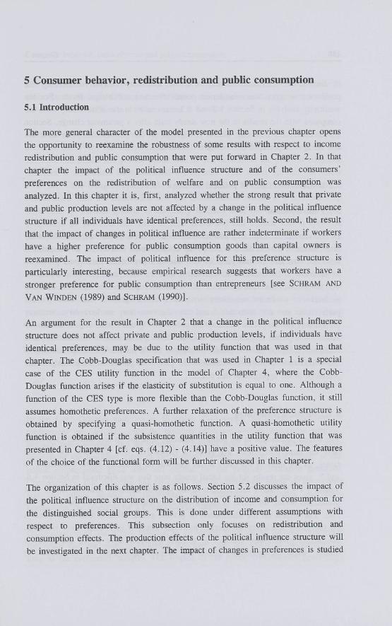
The effects of changes in the political influence structure in case that all individuals have the same preferences, are given in Tables 5.1 - 5.5. The first row in these tables, as for most of the other tables that will be presented in the Chapters 5, 6 and 7, gives the results for the initial steady state that was discussed in Section 4.6. Tables 5.1 - 5.5 show that changes in the political influence structure hardly alter production levels, the levels of capital and labor inputs, prices, and the income tax rate. The effects on the distribution of private goods, leisure, and, consequently, on the utility levels are substantial, however. Thus, if individuals have identical, homothetic preferences, changes in political influence have strong redistributive effects, while the production effects are limited. Apart from the restrictions on

Consumer behavior, redistribution and public consumption 189

preferences, the small production effects are due to the fact that income is redistributed through a lump-sum transfer system (compare the production effects for a tax system without a transfer system in Section 7.4).

Although the production effects are negligible, it is of interest to analyze why they occur at all. From the analytical model investigated in Chapters 2 and 3 it was obtained that public and private production do not depend on the political influence structure if consumers have identical preferences. This result appears to follow from the Cobb-Douglas specification that was chosen for the utility function in combination with the assumption that the redistribution system is a self-financing lump-sum tax-transfer system. If the utility function is of the Cobb-Douglas type, consumers do not alter the share of their (after-tax) full income that is spent on each private good and leisure if their full income changes, because preferences are homothetic. If individuals have identical preferences, these shares have the same value for every individual. A redistribution of income, that follows from a change in the political influence structure, has no effect on total demand for the different private commodities and leisure in that case, but only affects the distribution of these goods. Also, a change in the political influence structure does not affect the production level of the public consumption good if preferences are identical and represented by a Cobb-Douglas function. This follows immediately from the marginal value of the political interest function with respect to public commodities (which is equal to the sum of the marginal individual benefits). For the public consumption good, this marginal value in case of the CES utility function equals

~ = E, **,«£* Gs(trl U^ty" Pit) (5.1)

In the Cobb-Douglas case (7, = 0) utility Ufi) drops out of this equation. If preferences are identical, only the political influence weights are group specific. Because these weights sum up to unity, it follows from eq. (5.1) that under these restrictions the marginal value of the political interest function with respect to the public consumption good does not depend on the political influence structure. Consequently, this structure has no effect on the production levels in the private and the public sectors if individuals have identical preferences and these preferences are specified by a Cobb-Douglas function.

Generalization of the utility function to a (nested) CES utility function still gives the result that the political influence structure does not influence production, as long as the preference weights with respect to the public consumption good (aa)

190 Chapter 5

Table 5.1 Effects on capital and shadowprices of capital Change in political influence, identical homothetic preferences

/*cl' /*c2' ^ w K, K2 Ks Kp qi = q2 qP = q*

0.10,0.10,0.8 511.69 369.57 89.075 166.84 .36961 .002186

0.15,0.15,0.7 511.86 369.76 88.862 166.80 .36972 .002237

0.25,0.25,0.5 512.98 371.02 87.402 166.57 .37045 .002629

0.05,0.05,0.9 511.91 369.82 88.790 166.78 .36976 .002253

0.05,0.15,0.8 511.85 369.74 88.874 166.80 .36971 .002233

Table 5.2 Effects on labor demand and leisure Change in political influence, identical homothetic preferences

/*cl> Mc2- M w L, U Ls L P '.i '* K 0.10,0.10,0.8 236.10 327.93 121.04 52.629 .2623 .2623 .2623

0.15,0.15,0.7 236.19 328.12 120.76 52.622 .3963 .3963 .2288

0.25,0.25,0.5 236.83 329.41 118.84 52.576 .6645 .6645 .1618

0.05,0.05,0.9 236.22 328.18 120.67 52.617 .1291 .1291 .2956

0.05,0.15,0.8 236.19 328.11 120.78 52.622 .1293 .3963 .2622

Table 5.3 Effects on production and commodity prices Change in political influence, identical homothetic preferences

/*cl. /*c2> M w x, x. Gs Gp Pi P2

0.10,0.10,0.8 286.55 323.16 125.53 87.102 0.81242 0.86714

0.15,0.15,0.7 286.64 323.32 125.27 87.087 0.81224 0.86696

0.25,0.25,0.5 287.27 324.41 123.45 86.996 0.81103 0.86574

0.05,0.05,0.9 286.67 323.37 125.18 87.078 0.81218 0.86691

0.05,0.15,0.8 286.63 323.31 125.28 87.088 0.81225 0.86697

Table 5.4 Effects on special provisions and utility Change in political influence, identical homothetic preferences

Mcl> Mc2> /*w <*cl »c2 <TW uc, uc2 uw 0.10,0.10,0.8 -.30537 -.31124 .07708 2.19475 2.19475 2.19475

0.15,0.15,0.7 .06128 .05534 -.01458 3.07111 3.07111 1.96448

0.25,0.25,0.5 .79297 .78655 -.19744 4.69168 4.69168 1.48382

0.05,0.05,0.9 -.66984 -.67580 .16821 1.23953 1.23953 2.41806

0.05,0.15,0.8 -.66937 .05535 .07675 1.24101 3.07113 2.19364


Table 5.5 Effects on dividend, wage rate, taxes and value of the political interest function Change in political influence, identical homothetic preferences

•ci' f-a< Mw d, d2 PL Th T P

0.10,0.10,0.8 .38245 .38832 .64091 .24175 132.930 2.19475

0.15,0.15,0.7 .38249 .38843 .64072 .24136 132.686 2.24627

0.25,0.25,0.5 .38276 .38918 .63944 .23873 131.033 2.63849

0.05,0.05,0.9 .38250 .38846 .64065 .24123 132.602 2.26175

0.05,0.15,0.8 .38249 .38842 .64073 .24138 132.700 2.24241

are zero. Otherwise, private and public production are affected by the political influence structure. This follows from eq. (5.1), where utilities do not vanish for a CES utility function. Political influences are then 'weighted' with the reciprocal of the utility levels ( Up1 ), and affect the marginal value of the political interest function, even if consumers' preferences are identical. A similar weighting of political influences holds for the marginal value of the political interest function with respect to the public production good. The marginal individual benefits of the production good follow indirectly from dividend income and the public consumption good that depend on the level of the public production good.1

Although a change in the political influence structure affects private and public production levels, the effects are very small, compared to the distribution effects. The production effect, that follows from the change in the level of the public production good will be discussed in Section 6.2.2. In this section the redistribution effects and the production effect that follow from changes in the production of private and public consumption goods are examined.

The redistribution effects are easily explained. If the political influence of workers increases, more income will be transferred to workers, at the cost of the income of capital owners. The consumption of private goods and leisure by workers increases, while capital owners will consume less. The redistribution of private

1 Note that in case of Cobb-Douglas utilities the marginal value of the political interest function with respect to a production good still depends on the political influence structure, because not all groups benefit from this good through dividend income. Eq. (5.1) contains, therefore, only marginal individual benefits from dividend income for the social groups that receive such income. If the sum of the influence weights of these groups changes, the marginal value of the political interest function will change as well, leading to a change in the production level of the public production good.

192 Chapter 5

consumption leads to a higher utility level for workers and to a lower utility level for capital owners. The value of the political interest function (P) is, however, hardly affected by the redistribution of private consumption. The effect of a change in the political influence structure on the value of the political interest function is dominated by the production effects. It can be read from Table 5.5, that the value of the political interest function increases if the political influence is distributed more unequally over the social groups. To see this, eq. (5.1) is a good device. It follows from this equation that a social group has a higher weight in the marginal value of the political interest functions with respect to the public consumption good if ftjt/, " increases. Although an increase in political influence (/*,) leads to an increase in utility, it turns out that this weight increases if the political influence of a social group increases. It can be shown, however, that the sum of the weights lxiUi

l decreases if political influence is distributed more unequally. The marginal value of the political interest function with respect to the public consumption good is, thus, at a maximum if the political influence weights are in accordance with the numerical strengths. For this political influence structure public consumption reaches the highest level. The higher level of public consumption increases the value of the political interest function, for its marginal value is positive. However, the extra government expenditure for the additional public production is financed with a distortionary tax, which has a negative effect on the value of the political interest function. It turns out that this negative effect on the political interest function exceeds the positive public consumption effect. Therefore, the public consumption good reaches the highest level if the political influence structure corresponds to the numerical strengths, while the value of the political interest function is at the lowest level at this point. The economic interpretation of this result is that a representative individual of a social group is willing to offer a smaller share of its income for the finance of a public consumption good if income increases. The larger political influence of the individual's social group enables the members of this group to let the government produce a lower level of the public consumption good.2

2 Note that it is important that production levels and tax rates are both endogenously determined, to obtain a change in the value of the political interest function if the political influence structure changes. This value is not affected by a change in political influence if the government has to collect taxes for the finance of an exogenously given expenditure level. The mechanisms discussed in this respect still hold if the utility function is of the quasi-homothetic type that will be discussed at the end of this section.


The discussion thusfar focused on a shift in political influence between capital owners and workers. The same mechanisms are at work, however, if one group of capital owners is able to increase its political influence at the cost of the other group, while workers' political influence does not change. The results of such a political change are given in the last lines of Tables 5.1-5.5.

The absence of large effects on production levels for homothetic utility functions is a consequence of the constant shares of disposable full income a consumer spends on the different private commodities and leisure. A redistribution of income has no effect on private production in that case, as long as total income does not change, all consumers have the same preferences, there are no public goods, and the redistribution is through a lump-sum transfer system. In the model at hand, only the absence of public goods does not apply. The presence of public goods causes the small changes in the production levels that occur if the political influence structure changes. The utility function can be made more flexible by introducing subsistence levels, as in eqs. (4.12) and (4.14). We also investigated the effects of a change in the political influence structure for such a utility function. The values of the subsistence levels can be found in Table 5.A.2 of Appendix 5.A. It appeared, however, that the production effects of a change in the political influence structure are still negligible if subsistence levels are introduced in the utility functions. The reason for these small effects is that, although the introduction of subsistence levels makes the utility function non-homofhetic, the function is still quasi-homothetic.3 This implies that the share of the excess budget (disposable income minus expenditures on the subsistence levels) that is spent on a particular commodity does not change if disposable income changes. Redistribution of income that follows from the change in the political influence structure has, therefore, only a small effect on production levels if utilities are quasi-homothetic. The effects of a change in the political influence structure are now easily understood with the arguments already provided and will, therefore, not be discussed here.

It is beyond the scope of this thesis to investigate whether a further generalization of the utility function does lead to substantial changes in production levels if the political influence structure changes. Examples of non-homothetic utility functions are the generalized Gorman polar form as presented in BLUNDELL AND RAY (1982, 1984) and the translog demand functions as used in JORGENSON (1984). For these

3 Quasi-homothetic preferences give linear Engel curves. The difference with homothetic preferences is that the Engel curves do not start from the origin.

194 Chapter 5

utility functions, the demand function is nonlinear in income. In that case aggregate demand is not a function of aggregate income. Note that this would put a strong burden on the use of the concept of a representative individual. Under non-homothetic preferences a representative individual only exists if all individuals in the social group are equal.

5.2.3 Different preferences

An important result that follows from the previous analysis is that the value of the political interest function increases the more the political influence weights deviate from the numerical strengths of the social groups. In this section it will be examined whether this conclusion still holds if individuals of different social groups have different preferences. It is assumed that workers have a higher preference for leisure and for the public consumption commodity than capital owners. Capital owners in sector 1 and sector 2 have identical preferences. The values of the utility parameters are presented in Appendix 5.A. The steady state results for different political influence structures can be found in Tables 5.6-5.10.

If the political influence of workers rises, the government increases the transfers (special provisions) to workers at the cost of the income of capital owners. The redistribution of income from capital owners to workers leads to lower private consumption, because workers are willing to spend a larger share of their income for the finance of the public consumption good than capital owners. Although the level of the public consumption good increases, if workers' political influence increases, the change in this production level is not substantial when compared with the changes in the other production levels. This is due to the fact that the government can more effectively redistribute income through special provisions than through changes in public consumption. Therefore, the optimal level of public consumption is hardly affected by the political influence structure, as long as the government is able to redistribute income through special provisions. The consequences of a greater political influence of workers on production, capital formation and labor demand in the private sectors and the public consumption sector, can now easily be deduced from the effects on private and public consumption. The changes in the public production sector will be explained in Section 6.2.3.


Table 5.6 Effects on capital and shadowprices of capital Change in political influence while workers have a stronger preference for leisure and the public consumption good than capital owners

/*cl> A*-c2> A'w K, K2 Ks Kp q. = <b qP = <h

0.10,0.10,0.8 455.16 320.23 110.89 154.75 .36646 .003350

0.15,0.15,0.7 468.06 330.40 109.92 159.18 .36455 .003228

0.25,0.25,0.5 494.72 351.82 106.35 167.96 .36165 .003353

0.05,0.05,0.9 442.72 310.60 111.18 150.27 .36874 .003666

0.05,0.15,0.8 455.35 320.43 110.70 154.73 .36655 .003423

Table 5.7 Effects on labor demand and leisure Change in political influence while workers have a stronger preference for leisure and the public consumption good than capital owners

/*cl- Mc2> Mw L, U Ls Lp *.i la K 0.10,0.10,0.8 208.79 282.49 149.89 48.531 .2108 .2108 .3353

0.15,0.15,0.7 214.70 291.45 148.49 49.918 .3164 .3164 .2902

0.25,0.25,0.5 226.98 310.42 143.69 52.685 .5233 .5233 .2020

0.05,0.05,0.9 203.13 274.05 150.24 47.138 .1046 .1046 .3807

0.05,0.15,0.8 208.89 282.69 149.56 48.528 .1039 .3186 .3351

Table 5.8 Effects on production and commodity prices Change in political influence while workers have a stronger preference for leisure and the public consumption good than capital owners

Mcl> Mc2' Mw x, X2 Gs G P Pi P2

0.10,0.10,0.8 254.89 280.59 150.97 80.485 0.86440 0.92075

0.15,0.15,0.7 262.11 289.40 150.21 82.786 0.85281 0.90871

0.25,0.25,0.5 277.05 307.94 146.61 87.368 0.83001 0.88505

0.05,0.05,0.9 247.92 272.23 150.92 78.167 0.87585 0.93265

0.05,0.15,0.8 254.99 280.76 150.75 80.476 0.86415 0.92050

A less straightforward result is the decrease in the value of the political interest

function if there is a moderate increase in the political influence of capital owners

(the political influence weight for each group of capital owners increases from 0.10

to 0.15, while the workers' political influence weight decreases from 0.80 to 0.70;

see the second line in Table 5.10). This decrease is in contrast with the finding in

the previous section where the value of this function appeared to increase if the

196 Chapter 5

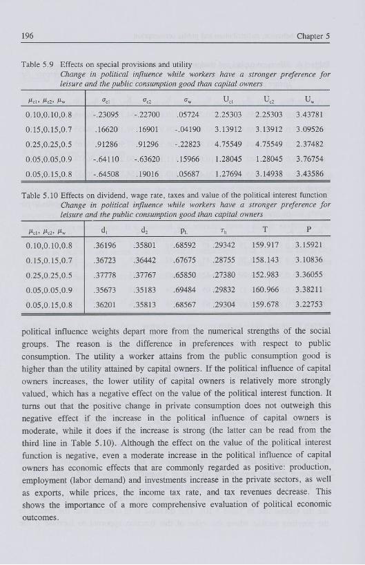
Table 5.9 Effects on special provisions and utility Change in political influence while workers have a stronger preference for leisure and the public consumption good than capital owners

Mel. Mc2> /*w °cl CC2 <?w uc, uc2 uw 0.10,0.10,0.8 -.23095 -.22700 .05724 2.25303 2.25303 3.43781

0.15,0.15,0.7 .16620 .16901 -.04190 3.13912 3.13912 3.09526

0.25,0.25,0.5 .91286 .91296 -.22823 4.75549 4.75549 2.37482

0.05,0.05,0.9 -.64110 -.63620 .15966 1.28045 1.28045 3.76754

0.05,0.15,0.8 -.64508 .19016 .05687 1.27694 3.14938 3.43586

Table 5.10 Effects on dividend, wage rate, taxes and value of the political interest function Change in political influence while workers have a stronger preference for leisure and the public consumption good than capital owners

f*cl> Mc2> M w d, d2 PL Th T P

0.10,0.10,0.8 .36196 .35801 .68592 .29342 159.917 3.15921

0.15,0.15,0.7 .36723 .36442 .67675 .28755 158.143 3.10836

0.25,0.25,0.5 .37778 .37767 .65850 .27380 152.983 3.36055

0.05,0.05,0.9 .35673 .35183 .69484 .29832 160.966 3.38211

0.05,0.15,0.8 .36201 .35813 .68567 .29304 159.678 3.22753

political influence weights depart more from the numerical strengths of the social groups. The reason is the difference in preferences with respect to public consumption. The utility a worker attains from the public consumption good is higher than the utility attained by capital owners. If the political influence of capital owners increases, the lower utility of capital owners is relatively more strongly valued, which has a negative effect on the value of the political interest function. It mms out that the positive change in private consumption does not outweigh this negative effect if the increase in the political influence of capital owners is moderate, while it does if the increase is strong (the latter can be read from the third line in Table 5.10). Although the effect on the value of the political interest function is negative, even a moderate increase in the political influence of capital owners has economic effects that are commonly regarded as positive: production, employment (labor demand) and investments increase in the private sectors, as well as exports, while prices, the income tax rate, and tax revenues decrease. This shows the importance of a more comprehensive evaluation of political economic outcomes.


5.3 Effect of changes in preferences

5.3.1 Introduction

Apart from the political influence structure, redistribution of income and public

consumption depends on the consumers' preferences, as specified by the utility

functions. The utility functions in the model presented in Chapter 4 contain three

types of parameters: preferences weights, substitution elasticities and subsistence

levels. In this section we analyze the effects of a change in the aforementioned

preference parameters. The analysis starts, in Section 5.3.2, with a discussion of

changes in the preference weights. The impact of substitution elasticities is studied

in Section 5.3.3. We also studied the effects of a change in the subsistence levels.

It followed, however, that these effects were rather straightforward. A higher

subsistence level increases the marginal utility of a particular consumption level.

An increase in the subsistence level has, therefore, a positive effect on the

consumption level of that good. The results of a higher subsistence level can now

easily be obtain if this mechanism is taken into account. Therefore, the effects of a

change in the subsistence levels are not discussed here.

5.3.2 The impact of changes in the preference weights of all groups

Preferences are represented by a nested utility function with a constant elasticity of

substitution between commodities that are in the same nest (see Section 4.3).

Preference weights represent preferences with respect to the components of a

composite commodity in a particular nest. The aggregated preference weight of a

commodity is then equal to the product of the preference weight on the lowest level

that the commodity appears and the appropriate preference weights on all higher

levels in the utility tree. In this section, the focus is not on these aggregate

preference weights, but on the preference weights as presented in Section 4.3. The

sensitivity analysis with respect to the preference weights concentrates on the

steady state effects. It is assumed that the preference change is equal for all

individuals.4 The main results are presented in Tables 5.11 - 5.15.

4 We also studied a change in the preference weights of workers while preferences of capital owners did not change. Compared to a change in the preference weights of all individuals, the effects on production of such a change were different in magnitude, but rather similar in sign. The effects on the distribution of income were different, but these differences are rather straightforward. Therefore, this analysis is not presented here.

198 Chapter 5

Table 5.11 Effects on capital and shadowprices of capital Change in preference weights of all individuals

<* c i , «H. <*Gi K, K2 Ks Kp qi = <h qP = q*

0.7 ,0.2 ,0.1 511.69 369.57 89.075 166.84 .36961 .002186

0.6 ,0.2 ,0.2 435.20 292.83 155.67 166.99 .33852 .005397

0.7 ,0.1 ,0.2 521.51 349.52 191.08 214.93 .30880 .004488

0.6 ,0.3 ,0.1 425.88 308.32 72.528 126.11 .40460 .002670

Table 5.12 Effects on labor demand, leisure and the wage rate Change in preference weights of all individuals

«ci . «(i> «Gi L, L2 Ls Lp ' i PL

0.7 ,0.2 ,0.1 236.10 327.93 121.04 52.629 .26230 .64091

0.6 ,0.2 ,0.2 196.28 253.98 206.77 51.492 .29147 .72559

0.7 ,0.1 ,0.2 232.87 300.14 251.29 65.614 .15009 .67929

0.6 ,0.3 ,0.1 199.17 277.29 99.892 40.321 .38333 .68355

Table 5.13 Effects on production and commodity prices Change in preference weights of all individuals

aci, aH, <*Gi x, X2 Gs Gp Pi P2

0.7 ,0.2 ,0.1 286.55 323.16 125.53 87.102 .81242 .86714

0.6 ,0.2 ,0.2 243.71 257.29 203.45 85.903 .89905 .95501

0.7 ,0.1 ,0.2 292.04 306.92 248.75 109.85 .83332 .88572

0.6 ,0.3 ,0.1 238.49 269.91 102.64 66.418 .87822 .93633

Table 5.14 Effects on special provisions, and taxes Change in preference weights

utility, the value of the political interest function

of all individuals

<*ci> « f , > <*Gi » c l <*c2 ff„ U,=P Th T

0.7 ,0.2 ,0.1 -.30537 -.31124 .07708 2.1948 .24175 132.93

0.6 ,0.2 ,0.2 -.28992 -.27044 .07005 5.2795 .37245 217.57

0.7 ,0.1 ,0.2 -.32216 -.29905 .07765 5.2815 .38239 250.46

0.6 ,0.3 ,0.1 -.27466 -.28077 .06943 2.2310 .23216 113.98


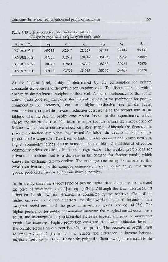
Table 5.15 Effects on private demand and dividends Change in preference weights of all individuals

«ci. ««. «Gi Cd» cfli Cd2i COi d, d2

0.7 ,0.2 ,0.1 .09253 .02947 .25667 .08973 .38245 .38832

0.6 ,0.2 ,0.2 .07258 .02672 .20247 .08125 .35996 .34049

0.7 ,0.1 ,0.2 .08723 .02881 .24319 .08763 .39981 .37670

0.6 ,0.3 ,0.1 .07665 .02729 .21387 .08305 .34409 .35020

At the highest level, utility is determined by the consumption of private commodities, leisure and the public consumption good. The discussion starts with a change in the preference weights on this level. A higher preference for the public consumption good (aGi increases) that goes at the cost of the preference for private commodities (aci decreases), leads to a higher production level of the public consumption good, while private production decreases (see the second line in the tables). The increase in public consumption boosts public expenditures, which causes the tax rate to rise. The increase in the tax rate lowers the shadowprice of leisure, which has a negative effect on labor supply. Although the decrease in private production diminishes the demand for labor, the decline in labor supply pushes up the wage rate. This leads to higher production costs and, consequently to higher commodity prices of the domestic commodities. An additional effect on commodity prices originates from the foreign sector. The weaker preferences for private commodities lead to a decrease in the demand for foreign goods, which causes the exchange rate to decline. The exchange rate being the numéraire, this entails an increase in the domestic commodity prices. Consequently, investment goods, produced in sector 1, become more expensive.

In the steady state, the shadowprice of private capital depends on the tax rate and the price of investment goods [see eq. (4.34)]. Although the latter increases, its effect on the shadowprice of capital is dominated by the negative effect of the higher tax rate. In the public sectors, the shadowprice of capital depends on the marginal social costs and the price of investment goods [see eq. (4.35)]. The higher preference for public consumption increases the marginal social costs. As a result, the shadowprice of public capital increases because the price of investment goods also increases. Higher production costs and the lower production levels in the private sectors have a negative effect on profits. The decrease in profits leads to smaller dividend payments. This reduces the difference in income between capital owners and workers. Because the political influence weights are equal to the

200 Chapter 5

numerical strengths of the social groups and preferences are identical, the government tries to equate after-tax income, which leads to a reduction in transfers to workers, compared to the initial steady state.

If the stronger preference for public consumption is accompanied by a decrease in the preference for leisure (aG, increases and af, decreases), labor supply will increase (see the third line in the tables). The positive effect on labor supply of the lower preference for leisure dominates the negative effect on labor supply that follows from the higher income tax, that is necessary for the finance of the extra government expenditures on the public consumption good. Compared with the earlier change, the government can now employ more public sector workers for the production of the public goods. The government is even willing to pay them a higher wage, because the higher demand for public goods positively influences the marginal benefits of labor input. The increase in the level of the public consumption good is, therefore, much stronger in this case. The strong increase in the production of the public consumption good has a positive effect on the production of the public production good. An expansion of the public production good can now be observed, which is not only the consequence of the strong increase in the level of the public consumption good, but also of the fact that private consumption decreases only moderately. The lower private consumption level leads to a decrease in imports and a smaller production level in private sector 2. Production in sector 1 increases, however, because of the increased government demand for investment goods (recall that the goods that are produced in this sector can be used for investment as well as consumption purposes). Labor demand decreases in both private sectors, however, which is due to the higher wage rate. The increase in commodity prices originates again in the foreign sector, as discussed above. The increase in production in private sector 1 has a positive influence on profits, while the decrease in production in private sector 2 negatively affects the profits in this sector. Consequently, dividend payments increase in sector 1 and decrease in sector 2. The impact on the redistribution of income through special provisions is now straightforward.

From a comparison of the above results with the results presented in Chapter 2 for an identical change in the preference weights, it follows that the effect on private production differs. The increase in the preference weight for the public consumption good and the simultaneous decrease in the preference weight for leisure led in Chapter 2 to an increase in private consumption (see the last columns


in Tables 2.2 and 2.3).5 For the model that is used in this chapter, the similar change in preference weights gives, in contrast, a decrease in private consumption. Production in private sector 1 only increases because the decrease in the consumer demand for this commodity is outweighed by the increase in investment demand.

The third preference change that is investigated concerns a higher preference for leisure (a(l increases) with a simultaneous decrease in the preference for private commodities (aci decreases). This preference change leads to a decrease in demand for private commodities and in labor supply (see the last line in the tables). The lower demand for private commodities leads to a decrease in private production and imports. Again, the reduced imports and the fixed exchange rate (the numéraire) push up the domestic commodity prices. Moreover, the lower labor supply boosts the wage rate. This leads to a decrease in the demand for labor in the public sectors, which negatively affects public production. There is an additional negative effect on public production that is less obvious. The preference weights are adjusted with the substitution parameters, as shown by eq. (4.12). This implies that, although the preference weights sum up to one, the adjusted preference weights do not necessarily do so. The preference change from private commodities to leisure leads to an increase in the sum of the adjusted preference weights. Therefore, the relative adjusted preference weight for public consumption decreases, although the preference weight for public consumption does not change. This has a negative effect on the level of the public consumption good. The other effects can now easily be understood.

The above results of a higher preference for leisure and an accompanying lower preference for private commodities differ in two respects from the results of a similar change in preferences that was investigated in Chapter 2. First, the commodity price decreases relative to the wage rate in Chapter 2, while it relatively increases in this chapter. In this chapter, the lower preference for private commodities reduces the demand for foreign commodities. The lower import of commodities goes with a lower export of commodities, which is realized by an increase in the prices for domestic commodities. This effect is absent in the model

5 In Chapter 2 the effects were analyzed for a change in preference weights for one social group, while the preferences of the other social group did not change, while the preference change that is analyzed in this chapter holds for all social groups. If, however, only the preference weights of workers are altered, the effects on production and input levels have the same sign as they have if the change in preference weights occurs for all social groups.

2 0 2 Chapter 5

for a closed economy of Chapter 2. Second, the change in preference weights has no effect on the tax rate in the model of Chapter 2, while it has a negative effect on the tax rate in this chapter.6 Because the change in preferences does not affect the preference weight for public consumption, this change does not alter the share of income that consumers are willing to spend on public consumption in the model of Chapter 2. In the model of this chapter, the decrease in the preferences for private commodities has a negative effect on the level of the public production good. The decrease in the production of this good is stronger than the decrease in the public consumption good. Furthermore, public consumption faced, compared with Chapter 2, an additional negative effect, because of the aforementioned decrease in the relative adjusted preference weight for public consumption. These two effects make that the change in the preference weights leads to a decrease in the tax rate.

At the next level in the utility tree, private commodities are split up in commodities of type 1 and commodities of type 2. The results of a change in the preference weights concerning these two types of commodities is rather straightforward and will, therefore, not be reproduced in the tables. The main effects can be summarized as follows. A higher preference for commodities of type 2 (a2, increases) at the cost of the preference for commodities of type 1 (au decreases), leads to an increase in the demand for domestic and foreign commodities of type 2 and a decrease in the demand for domestic and foreign commodities of type 1. The price of commodity 2 then increases and the price of commodity 1 decreases. These changes in prices positively affect the export of domestic commodity 1, while the export of the other commodity is negatively affected. Furthermore, the lower price of commodity 1 makes investment goods cheaper. Labor will then be substituted by capital, which is, in particular, notable in the public production sectors. The production levels in these sectors increase a little, but the increase in capital stocks and decrease in labor demand is more substantial. The lower investment costs make a reduction of the tax rate possible. The decrease in the production level and in the commodity price of sector 1 leads to lower profits and dividend payments in this sector. For sector 2 the opposite holds. More income from capital owners in sector 2 and less income from capital owners in sector 1 is then transferred to workers through special provisions.

6 The negative signs for the effect on the tax rate in Tables 2.2 and 2.3 go to zero if the change in preference weights does not affect the preference weight for the public consumption good, as can easily be obtained from eq. (2.23).


The lowest level of the utility tree decomposes the commodity bundles of type 1 and type 2 into a domestic commodity and a foreign commodity. A higher preference for a domestic commodity at the cost of the preference for the foreign commodity of the same type pushes up the prices of both domestic commodities. The higher price of commodity 1 leads to an increase in investment costs, which reduces the public capital stocks. Public production levels are, however, hardly affected by the change in preference weights on the lowest level of the utility tree. The higher domestic commodity prices have, furthermore, a positive effect on profits, that offsets the negative effect on profits of the higher per capita costs of labor and investments. The concomitant increase in dividend payments in both sectors induces the government to transfer more income from entrepreneurs to workers in order to equalize disposable income.

5.3.3 The impact of changes in the substitution elasticities of all groups

As noticed in Section 4.2, an interesting feature of a nested utility function is the possibility to allow for differences in substitutability between goods. The utility function used in this chapter comprises three different substitution parameters: 7,, specifying the substitutability between private commodities, leisure and the public good; yci, specifying the substitutability between private commodities of type 1 and of type 2; and ycji, specifying the substitutability between domestic and foreign commodities of type j . In this section the impact of the distinct substitution parameters is discussed. This is done by analyzing the effects of a change in substitution parameters that is identical for all (representative individuals of) social groups.7 The results for the different cases that are studied are summarized in Tables 5.16-5.19.

An increase in the substitution elasticities makes the demand for commodities more sensitive to prices. From the demand equations it can be derived that such an increase leads to an increase (decrease) in the demand for a commodity if the price of this commodity is low (high), relative to the prices of the other commodities.

7 As for the preference weights, it was also analyzed what the effects are if only the substitution parameters for workers alter. The effects on production from this change differ only in magnitude from the effects of a change in the substitution parameters for all social groups, while the differences in the redistribution of income are straightforward. Therefore, the effects of a change in the substitution parameters for workers can easily be obtained from the analysis of a change in the substitution parameters for all social groups.

204 Chapter 5

Table 5.16 Effects on capital, shadowprices of capital and price of commodity 1 Changes in substitution elasticities

/ i» T e n Tcji K, K2 Ks Kp qi=q 2 qs=qP Pi

0.1, 0.1, 0.3 511.69 369.57 89.075 166.84 .36961 .00219 .81242

0.1, 0.1, 0.7 508.56 372.43 89.116 167.11 .39188 .00221 .86117

0.1, 0.3, 0.7 510.43 371.09 89.049 167.02 .39213 .00221 .86168

0.3, 0.3, 0.7 318.54 165.61 269.24 170.62 .25023 .00844 1.0804

0.3, 0.3, 0.1 313.42 171.12 270.40 171.59 .26932 .00845 1.1602

0.3, 0.2, 0.1 313.11 171.31 270.46 171.61 .26932 .00845 1.1602

Table 5.17 Effects on production, exports and price of commodity 2 Changes in substitution elasticities

Yi, Tci, Tcji x, X2 Gs Gp E, E2 P2

0.1, 0.1, 0.3 286.55 323.16 125.53 87.102 75.755 66.495 .86714

0.1, 0.1, 0.7 284.80 325.18 125.49 87.182 67.421 59.003 .92055

0.1, 0.3, 0.7 285.84 324.26 125.46 87.168 67.340 59.025 .92038

0.3, 0.3, 0.7 178.38 148.61 320.63 85.148 42.832 39.598 1.1237

0.3, 0.3, 0.1 175.52 152.77 321.20 85.460 37.145 33.985 1.2129

0.3,0.2,0.1 175.34 152.90 321.23 85.463 37.145 33.970 1.2132

Table 5.18 Effects on private demand, leisure, utility, the value of the political interest function and the wage rate Changes in substitution elasticities

Ti> T c i ' Tcji C d l i Cfli Cd2i Cf2i i; U,=P PL

0.1, 0.1, 0.3 .09253 .02947 .25667 .08973 .26230 2.1948 .64091

0.1, 0.1, 0.7 .09910 .02581 .26618 .08657 .26186 2.2211 .68010

0.1, 0.3, 0.7 .10019 .02614 .26524 .08620 .26188 2.2213 .68011

0.3, 0.3, 0.7 .03945 .02188 .10902 .06892 .33427 8.0074 .91363

0.3, 0.3, 0.1 .04200 .02123 .11877 .06308 .33212 8.0627 .98407

0.3, 0.2, 0.1 .04184 .02115 .11893 .06318 .33217 8.0636 .98422


Table 5.19 Effects on dividends, special provisions and taxes Changes in substitution elasticities

Ti' Tci' Ycji d, d2 Th T cl "c2 CTW

0.1, 0.1, 0.3 .38245 .38832 .24175 132.93 -.3054 -.3112 .07701

0.1, 0.1, 0.7 .40292 .41481 .24158 141.03 -.3211 -.3330 .08177

0.1, 0.3, 0.7 .40464 .41326 .24154 141.02 -.3228 -.3317 .08182

0.3, 0.3, 0.7 .31663 .23141 .61401 407.12 -.2618 -.1766 .05480

0.3, 0.3, 0.1 .33454 .25678 .61310 439.17 -.2756 -.1978 .05917

0.3, 0.2, 0.1 .33421 .25706 .61311 439.24 -.2751 -.1979 .05913

Consider first an increase in the substitution parameter ycji (see the second line in each table), and, thus, in the substitution elasticity between domestic and foreign goods of type 1 and of type 2.8 This leads to an increase in the demand for the two domestic commodities and to a decrease in the demand for the two foreign commodities, because the domestic commodity prices are lower than the foreign prices (which are equal to one). The larger demand for domestic commodities leads to an increase in the domestic commodity prices, which has a negative effect on exports. The decrease in exports of commodities produced in sector 1 is so strong that it dominates the extra domestic demand for this good, which leads to a lower production in this sector. For sector 2 the extra domestic demand dominates, leading to a higher production level in sector 2. The higher prices for the domestic commodities have a positive effect on profits, allowing the firms to increase their dividend payments. Although the smaller production in sector 1 has a negative effect on labor demand, total labor demand increases, because this negative effect is outweighted by the extra labor demand in the more labor intensive sector 2. The impact of the change in the substitution elasticity between domestic and foreign goods of type 1 and of type 2 on public production is negligible.

If, in addition, the substitution elasticity between private commodities of type 1 and type 2 increases, a similar effect is observed. The demand for the composite good with the higher price (good 2) decreases in favor of the demand for the composite good with the lower price (good 1). Also the effect on prices is analogous: the

8 Recall that the relation between the substitution elasticity a and the substitution parameter y is given by a = l/(l-y). Nonnegativity of the substitution elasticity requires that 7 < 1.

206 Chapter 5

difference between the price of composite good 1 and composite good 2 is reduced. More specifically, the price of domestic commodity 1 increases, while the price of domestic commodity 2 decreases. The higher price of commodity 2 has a positive effect on the sector's profits, while the lower price of commodity 1 reduces the profits in sector 1. Although the lower price of domestic commodity 2 has a positive effect on export, production in sector 2 decreases, which leads to a decrease in labor demand. The extra labor demand in sector 1 cannot prevent total labor demand from falling. Leisure then increases. The impact on public production is not substantial.

The changes in the substitution parameters discussed so far particularly affected the demand for private commodities and prices. The impact on the labor market and on public production was not substantial. This changes if, in addition, the substitution parameter on the highest level of the utility tree increases (y, increases: see the fourth line in the tables). The higher substitution elasticity leads, again, to an increase in the consumption of the commodity with the lowest price. The public consumption good has the lowest (shadow-)price. An immense increase in the level of the public consumption good can be observed. The demand for private goods decreases enormously, because the composite of private goods has the highest price. The reduction in price differences can also be observed for this case. The prices of the domestic private goods do increase, but the initially lower price of the public consumption good increases much stronger. The strong increase in the income tax rate cuts, however, the shadowprice of leisure, which is equal to (l-Th)pL. Labor supply then decreases, but total labor demand also falls because of the immense reduction in private production which is due to the strong decrease in the demand for private commodities. The decrease in the production levels has, furthermore, a negative effect on profits, which cannot be offset by the higher commodity prices. The lower profits reduce the dividend payments. To achieve the desired distribution of incomes, lower special provisions will suffice. Utilities are positively influenced by the change in the substitution parameter on the highest level of the utility tree.

Substitution between (composite) goods was, in the above cases, easier between commodities on a lower level of the utility tree. An increase in the substitution parameter led to an increase in the consumption of the commodity with the lowest price. It appears that this mechanism is still at work if the values of the substitution parameters are larger at a higher level of the utility tree. If, for example, the values of the substitution parameters between domestic and foreign commodities


decrease, for type 1 and type 2 commodities, and become smaller than the values of the substitution parameters for the higher levels on the utility tree (ycli and yc2i

become smaller than yd and yt: see the fifth line in the tables), consumption of the commodity with the lowest price decreases, while the consumption of the commodity with the highest price increases. The foreign commodities are cheaper than the domestic commodities, which leads to a lower demand for foreign commodities. The resulting decrease in exports is so strong that it outweighs the increased domestic demand for this good, and causes production in sector 1 to decrease. As a consequence, the price of commodity 1 increases, which leads to an increase in the difference between the domestic and foreign commodity of type 1. The decrease in exports of commodity 2 does not outweigh the higher domestic demand for commodity 2. Production in sector 2 increases, which leads to a decrease in its price. The higher revenues that are obtained in both private sectors have a positive influence on profits and dividends. The higher revenues, furthermore, allow for a higher wage rate, because the Cobb-Douglas production function implies a constant expenditure share for labor costs in both sectors.

The substitution parameters in the above cases were all positive, which gives substitution elasticities between commodities in the same nest that are greater than one. Substitution elasticities greater than one do not guarantee that commodities, that are not on the same level of the utility tree, are (gross) substitutes. However, it can be shown [see e.g. KELLER (1976)], that all commodities are gross substitutes if the substitution elasticity on the highest level is greater than, or equal to, one and the substitution elasticity does not decrease if a lower level on the utility tree is reached.9 Analogously, sufficient conditions for complementarity are a substitution elasticity smaller than or equal to one at the highest level together with a smaller substitution elasticity for the lower levels.10 It turns out that the effects of a decrease in the Subsumtion elasticities to a value smaller than one (to negative values of the substitution parameters) are still dominated by the mechanism that a decrease in the substitution elasticity leads to a decrease in the consumption of the commodity with the lower price. These effects are now rather straightforward and are, therefore, not further discussed here.

9 The condition on the substitution parameters for gross substitutability is, thus, 0 < 7, < yci < yci, j = 1, 2, where at least one strict inequality must apply.

10 Complementarity is obtained if the following conditions for the substitution parameters are fulfilled: ycß < yd < T, ^ 0, j = 1, 2, where one strict inequality must hold.

208 Chapter 5

5.4 Transition effects of changes in political influence and preferences

5.4.1 Introduction

The analyses of changes in the political influences structure and preferences, as discussed in the previous sections, concentrated on the long run effects. These effects were obtained by comparing the steady state solution for the initial parameter set with the steady state solution that holds for the changed parameter set. In this section, the focus is on the transition path that the economy follows before it reaches the new steady state. In the steady state future values of variables are equal to their present values. Therefore, expected values of variables can be set equal to the present values. Along the transition path, future and present values of variables are not necessarily equal. An expectation rule must be defined before the dynamic paths can be solved. Although steady state outcomes do not depend on the expectation rule that agents have (see Section 4.7), the transition path does depend on the expectation rule agents have with respect to future variables that influence current decisions.

In the model presented here, the investment decisions of entrepreneurs and the government depend on the expected benefits of investments. These expectations are reflected by the shadowprice of capital for the next period (q/t+l), j = 1, 2, p, s). These shadowprices are the only variables for which agents must hold expectations. It is assumed here that agents have static expectations, given by:

Efe/f+1), t] = qff), j = 1, 2, p, s (5.2)

where the expectations indicator refers to the value of variable q} in period f+7 as it is expected in period t. In Section 4.7 we compared the static expectation rule with other expectation rules. In this chapter, as well as in Chapters 6 and 7, we will only give transition effects for the static expectation rule. The transition effects for other expectation rules can easily be obtained with the results given in this section and Section 4.7.

We concluded in Section 5.2, that changes in political influence hardly affect the private and public production levels if individuals have identical preferences. Significant effects on production can be obtained, however, if differences in preferences are allowed. In order to get an interesting analysis of transition paths, the original parameter set is adapted in this way. A second change in the parameter set concerns a stronger impact of the public production good (infrastructure) on the


production in private sector 1. The complete parameter set that is used in this section is given in Appendix 5.A.2.

Transition effects will be investigated for three different parameter changes. Section 5.4.2 discusses the effects of a change in the political influence structure, implying a rise in the influence of workers, at the cost of the political influence of both groups of capital owners. In Section 5.4.3 we investigate the transition path after a change in the preferences of workers, which involves an increase in their preference for the public consumption good. Finally, the effects of a simultaneous change in the political influence and preferences of workers is discussed in Section 5.4.4.

5.4.2 Change in political influence structure

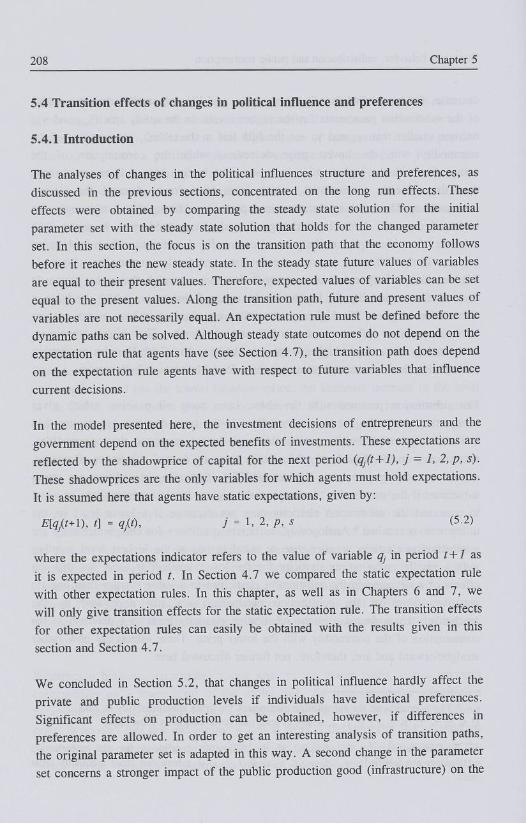
The transition paths of the key variables are presented in Figures 5.1 - 5.8. These figures show the deviations from the initial steady state values. Using deviations gives us the opportunity to present the transition paths of several variables in one figure. The discussion of the transitional effects of a change in the political influence structure starts with the initial effects that immediately follows the change in influence.

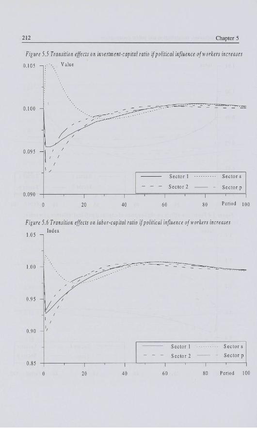
The increase in political influence of workers leads to a change in the redistribution of income by the government, in favor of the workers.11 Workers have a stronger preference for the public consumption good than capital owners and are, consequently, willing to pay higher taxes for the finance of extra production of this good. This induces the government to increase the production of the public consumption good (cf. Figure 5.3). The higher production level requires an increase in labor and capital input, and an expansion of the public production good (infrastructure). The adjustment of the level of the capital stock and of infrastructure takes some time. However, the government can increase the production of public consumption immediately by employing more workers (cf. Figures 5.1 and 5.2; the development of the labor-capital ratio is presented in Figure 5.6, while Figure 5.7 gives the development of labor productivity). In

11 The shock that is discussed here implies a strong change in the political influence weights, leading to new weights that are equal to ^w = 0.96 (instead of 0.80) and fici = 0.02 (instead of 0.10) for j = 1,2.

210 Chapter 5

Figure 5.1 Transition effects on capital stocks if political influence of workers increases

1.08 -i Index

Period 100

Figure 5.2 Transition effects on labor demand if political influence of workers increases

Index 1.04 -,

1.00 -

0.96

0.92 -

0.88

0.84

20 40

Sector 1

Sector 2

Sector s

Sector p

60 Period 100


Figure 53 Transition effects on production if political influence of workers increases

1.04 -i Index

1.00

0.96 -

0.92

0.88

20 40

Sector 1 Sector s

Sector 2 - Sector p

0 - r 60

T

Period 100

Figure 5.4 Transition effects on shadowprice of capital if political influence of workers increases

1.6 - i Index

1.4 -_ _ - - . r r r^ - -_ _ - - . r r r^ - -

1.2 -s

/ /

f - - __-___=_ 1.0 -

f - - __-___=_

" V^-^s 0.8 - / /

-- - -

oeciui s Sector p - - -

Sec tu i 2

oeciui s Sector p

n f, ' 1 ' 1 1 1 1

20 40 60 Period

212 Chapter 5

Figure 5.5 Transition effects on investment-capital ratio if political influence of workers increases

0.105 -..-"-. V a l u e

0.100

0.095

0.090

Sector 1 Sector s

- Sector 2 - Sector p

20 40 60 Period 1Q0

Figure 5.6 Transition effects on labor-capital ratio if political influence of workers increases Index

1.05

1.00

0.95

0.90

0.85

Sector 1 Sector s

Sector 2 - Sector p

20 60 Period 100


Figure 5.7 Transition effects on labor productivity if political influence of workers increases

1,04 T-i Index

1.02

1.00

0.98

0.96

Sector 1

Sector 2

Sector s

Sector p

1

0 20 40 60 Period i(

Figure 5.8 Transition effects on utility levels and value of political interest function (P) if political influence of workers increases

1.4 —i Index

1.2

1.0

0.8

0.6

0.2

0.0

Cap. owners 1 Cap. owners 2

20 40 60

Workers

Value P

Period 100

214 Chapter 5

addition, the government raises investments in the capital stock that is needed for the production of the public consumption good (Figure 5.5). For these extra investments the government is willing to pay a higher price, which shows up in the higher shadowprice of capital (qs; cf. Figure 5.4).

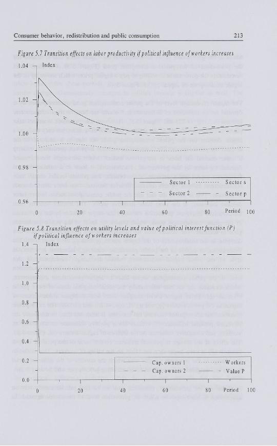
The higher production level of the public consumption good is accompanied by a demand for an expansion of infrastructure, because the benefits from infrastructure increase [cf. eq. (4.22) and Figure 5.3]. However, this expansion does not take place, because the increase in the political influence of workers not only leads to a higher demand for the public consumption good, but also to a decrease in the demand for private goods. The concomitant decrease in private production leads to a lower demand for labor in the private sectors, which outweighs the increased demand for labor by the government. Furthermore, it leads to a smaller demand for private capital and a decrease in the benefits that private sectors obtain from infrastructure. In spite of this decrease in labor demand, total labor demand tends to increase. This is due to the fact that the public consumption sector, where labor demand increases, is the most labor intensive sector. The smaller benefits from infrastructure in private production outweigh the larger benefits in the production of the public consumption good, which causes the level of the public production good to decrease. The smaller need for capital in the two private sectors leads to a decrease in the shadowprices of the capital stocks (q2 and q2; cf. Figure 5.4). The shadowprice of capital in the public production sector (qp) increases, however, in spite of the lower capital requirement, which discourages investments in this sector. The reason for the increase in this shadowprice is that the higher production level in the public consumption sector leads to higher government expenditures, which increases the tax rate and thereby the social marginal costs of extra public revenues (£)• These higher social marginal costs lead to higher shadowprices of capital in the public sectors [qp and qs; cf. eqs. (4.26) and (4.35)]. The extra public revenues that are required increase the tax rate. It turns out that, in this case, the increased political influence of workers has a positive influence on the utility of workers, and a negative influence on the utilities of capital owners (cf. Figure 5.8). The effect of the change in political influence on the value of the political interest function (P) is even larger than the effect on the utility of workers. This is due to the change in the influence weights with which the utilities of the different social groups are weighted in the political decisionmaking process (see also Section 5.2).

As holds for the government, producers must in the first periods mainly rely on adaptations in labor input to adjust the production level to the altered demand. In


addition, investment increases to adjust the capital stock, which takes time. In the first few periods, the effects of the political influence change are largely related to a redistribution of income, which changes the demand for goods, and to changes in labor input. After these periods, income redistribution and the demand for goods hardly change. Consequently, changes in utilities become negligible as well. The economic effects of the change in the political influence structure are then mainly related to the developments that take place on the production side, and the adjustments in the capital stocks. Capital stocks reach their new steady state value after approximately 100 periods (cf. Figure 5.1). In the first periods after the political influence change investment in the public consumption sector grows rapidly. Even overinvestment occurs in the sense that the capital stock increases to a level that is higher than the new steady state level. This is followed by a decline in investments which leads, with a time-lag, to a decrease in the capital stock (see also Figure 5.5). The (static) expectation rule that the government maintains with respect to the shadowprice of capital underlies the overinvestments in this sector, as explained in Section 4.7.

In contrast with the public consumption sector, the change in the political influence structure has a negative effect on the capital stocks in the private sectors and the public production sector, which leads to lower investments in these sectors. In fact the decrease in investments is so strong that, after a while, underinvestment occurs, leading to a level of the capital stock that is lower than the new steady state value (see Figures 5.1 and 5.5). This effect is most prominent in private sector 1. This sector shows also the smallest initial adaptation in investment and, as a consequence, the largest change in investment and production during the remainder of the transition path. This is not so surprising, because the goods of this sector are not only used for consumption but also for investment, and the adjustment in the demand for investment goods (or capital) proceeds more slowly than the adjustment in the demand for consumption goods. The shadowprices of capital in the two private sectors recover after the first periods, as excess capital wears out and is not replaced by new capital (cf. Figure 5.4). This increases the marginal benefits of capital and, consequently, the price capital owners are willing to pay for extra capital.

An opposite effect occurs in the public consumption sector. There, the change in the political influence structure leads to a higher demand for the public consumption good, for the production of which the government needs extra capital. The marginal benefit of capital increases, therefore, and the government is willing

216 Chapter 5

to pay a higher price for extra capital. Through higher investments the capital deficiency disappears, which reduces again the marginal benefit of capital and thus the price that the government is willing to pay for extra capital. In the public production sector the development of the shadowprice of capital is dominated by the social marginal cost of extra public revenues, which tends to increase over the whole period (cf. Figure 5.4).

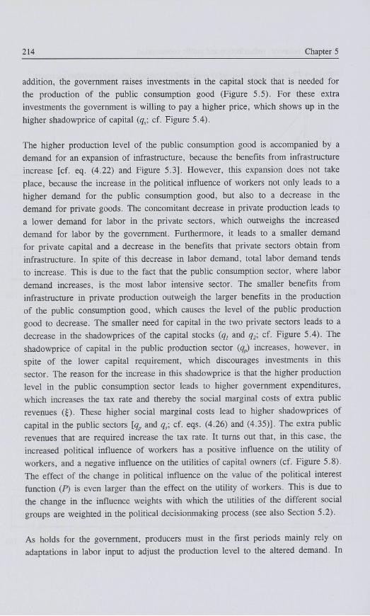
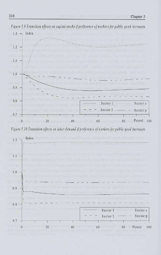
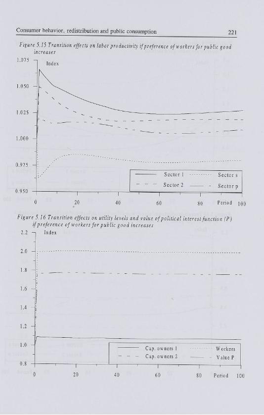
5.4.3 Change in workers' preference for the public consumption good

In case of a stronger preference of workers for the public consumption good the government is induced to increase the production of the public consumption good.12 On the other hand, the simultaneous decrease in the preference for private goods causes the demand for private goods to decrease. The transition paths for this preference change are presented in Figures 5.9 - 5.16. For convenience, the effects of this preference change are decomposed into effects concerning the production levels and the total demand for goods and factor inputs, on the one hand, and effects concerning redistribution and utilities on the other hand. It turns out that the transitional effects of the preference change on the production levels have the same direction as the effects discussed above for a change in the political influence structure in favor of workers (compare Figures 5.3 and 5.11). These results will not be repeated here.

With respect to the redistribution of income and the utility levels, the effects differ substantially from the effects that followed a political influence change (compare Figures 5.8 and 5.16). The main reason for this dissimilarity is the different impact that the two shocks have on the redistribution of income through transfers (special provisions). Larger political influence of workers led to an increase in their special provisions at the cost of the special provisions for capital owners. As a consequence, capital owners not only had to contribute to the extra production of the public consumption good, through a higher income tax, but were also confronted with higher taxes in form of special provisions that restricted their disposable income substantially. The resulting strong decrease in their private consumption and leisure overshadowed the extra utility received from the higher

The preference change of workers that is analyzed here consists of an increase in stribution parameter aGw 1

parameter <xc„ from 0.50 to 0.40.


level of the public consumption good, which led to a lower utility level for capital owners.

A change in the preference of workers again leads to a higher income tax for the finance of the extra public production. However, workers must now pay a price for the contribution of capital owners to the extra costs of public production. This contribution is realized by transferring income from workers to capital owners through the redistribution system. This enables capital owners to consume more of all private goods and to reduce their labor input. Together with the higher level of the public consumption good, this leads to higher utility levels for capital owners. Although workers are confronted with a reduction in the consumption of private goods, their utility levels also increase, because their leisure increases as well as the level of the public consumption good which is now more preferred by workers. The fact that all groups receive a higher utility, and the political influence weights do not change, implies that the value of the political interest function increases. The new situation is Pareto superior to the situation that existed before the preference shock. The redistribution effects mainly occur in the first periods after the preference change, as was also the case for the change in political influence.

5.4.4 Simultaneous increase in the political influence of workers and their preference for the public consumption good

A simultaneous change in the preference for the public consumption good and the political influence of workers is of interest, for the following reason. An increase in the preference for the public consumption good induces an increase in the number of public sector workers, at the cost of the number of private sector workers. Because there are good reasons to expect that the political influence of public sector workers is more strongly related to numerical strength than the influence of private sector workers,13 the increase in the number of public sector workers may also lead to an increase in the political influence of workers. Therefore, an increase in the workers' preference for public consumption may be accompanied by an increase in the political influence of workers. The transition paths for this simultaneous change are presented in Figures 5.17 - 5.24. Since the

13 Reasons for this difference are that public sector workers are better organized and that they can also influence the political decisionmaking process from within the governmental organization.

218 Chapter 5

Figure 5.9 Transition effects on capital stocks if preference of workers for public good increases

1.3 —| Index

1.2 -

1.1

0.7

Sector 1 Sector s

Sector 2 - Sector p

60 0 20 40 60 80 Period 100

Figure 5.10 Transition effects on labor demand if preference of workers for public good increases

Index 1.2

1.1

1.0

0.9 -

0.8

0.7

20 40

Sector 1 Sector s

Sector 2 - Sector p

"1 ' 1 80 Period 100 60


Figure 5.11 Transition effects onproiuction if preference of workers for public good increases

1.2 —i Index

1.1

1.0 -

0.8

0.7

Sector 1 Sector s

Sector 2 - Sector p

"i ' r 40 60

T

0 20 Period 100

Figure 5.12 Transition effects on shadowprice of capital if preference of workers for public good increases

3.5 -,

3.0

2.5

2.0

1.5

1.0

0.5 -

0.0

Index

0 20 40

Sector 1 •-• Sector s

Sector 2 - Sector p

T

Period 1(

220 Chapter 5

Figure 5.13 Transition effects on investment-capital ratio if preference of workers for public increases

013 _, Value

0.12 -

0.11 -

0.10

Sector 1 Sector s

Sector 2 - Sector p

0 20 40 60

— ' 1 Period 100

Figure 5.14 Transition effects on labor-capital ratio if preference of workers for public good increases

1.2

1.1

.0 -

Index

0.9

~r 20

Sector 1 Sector s

Sector 2 - Sector p

40 60 T

Period 100


Figure 5,15 Transition effects on labor productivity if preference of workers for public good increases

1.075 -, Index

1.050

1.025

1.000

.975

0.950

0 20

Sector 1

Sector 2

60

Sector s

Sector p

I Period i(

Figure 5.16 Transition effects on utility levels and value of political interest function (P) if preference of workers for public good increases

2.2 —| Index

2.0

1.6

1.4 -

1.2 -

1.0

0.8

r

20 40

Cap. owners 1 - Cap. owners 2

- i 1 r

60

Workers

Value P

Period 1(

222 Chapter 5

Figure 5.17 Transition effects on capital stocks if political influence of workers and preference of

workers for public good increase

1.4

Sector 1 Sector s

Sector 2 - Sector p

T ~~' 1

Period 10(

Figure 5.18 Transition effects on labor demand if political influence of workers and preference

of workers for public good increase

Index 1.2 -i

1.1 -

1.0

0.9

0.8

0.7

0.6

0.5

20 40

Sector 1

Sector 2

60 80

Sector s

Sector p

Period 1(

223 Consumer behavior, redistribution and public consumption

Figure 5.19 Transition effects on production if political influence of workers and preference of workers for public good increase

1.2 -i

1.1

1.0 - t

0.9 -

0.8

0.7 -

0.6

Index

0.5 -i

Sector 1

Sector 2

Sector s

Sector p

20 40 60 Period i(

Figure 5.20 Transition effects on shadowprice of capital if political influence of workers and preference of workers for public good increase

5.0

.0 -

3.0

2.0

0.0

Index

S e c t o r l •-•• Sectors Sector 2 - Sector p

Period 100

224 Chapter 5

Figure 5.21 Transition effects on investment-capital ratio if political influence of workers and preference of workers for public good increase

Value

0.13 -. '" ' \

0.12

0.11 - :

0.10

0.09

O.OS I /

0 20

Sector 1 Sector s

Sector 2 - Sector p

40 60

- ' 1 Period 1Q0

Figure 5.22 Transition effects on labor-capital ratio if political influence of workers and preference of workers for public good increase

1.2

1.1 -

1.0

0.9

0.8

0.7

0.6

Period 100


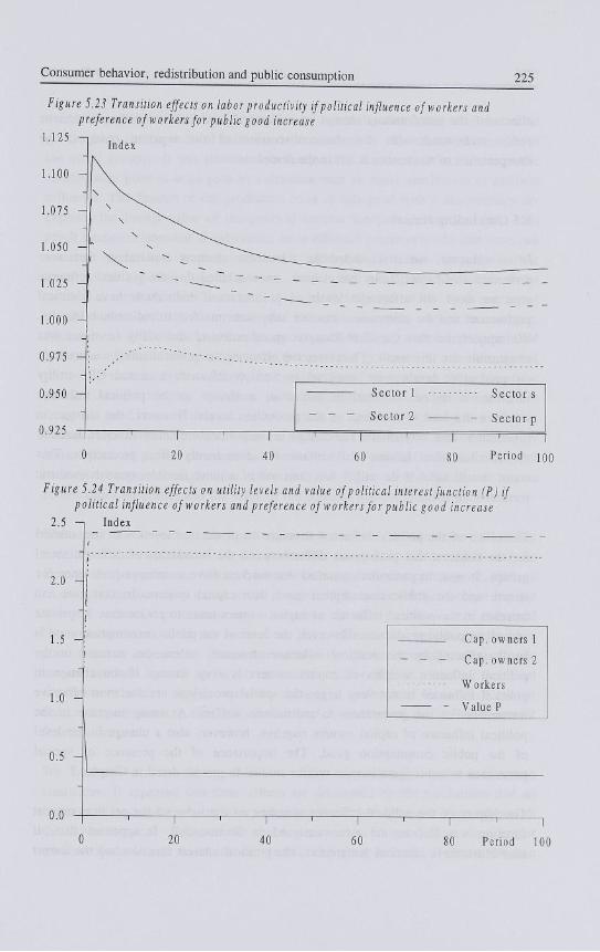
Figure 5.23 Transition effects on labor productivity if political influence of workers and preference of workers for public good increase

1.125

1.100 -

1.075 -

1.050 -

1.025

1.000

0.975

0.950

0.925

Index

Sector 1

Sector 2

Sector s

Sector p

20 40 60 Period \(

Figure 5.24 Transition effects on utility levels and value of political interest function (P) if political influence of workers and preference of workers for public good increase

2.5

2.0

1.5

1.0 -

0.5 -

Index

0.0

Cap. owners 1

- - Cap. owners 2

- Workers

— - Value P

~r 20

r 40 60 80 Period 100

226 Chapter 5

effects of the simultaneous change in preferences and political influence can be easily understood with the above discussion of the separate changes, the interpretation of the results is left to the reader.

5.5 Concluding remarks

In this chapter, we first studied the robustness of some conclusions that were arrived at in Chapter 2. In that chapter, we concluded that the political influence structure does not affect the levels of production if individuals have identical preferences and the government can use lump-sum transfers to redistribute income. We conjectured that the Cobb-Douglas specification of the utility functions was responsible for this result. Therefore, the effect of the political influence structure on production levels were analyzed in Section 5.2 with a nested CES utility function. It turned out that, in that case, a change in the political influence structure did lead to a change in the production levels. However, the changes in production were very small. The change in the political influence structure leads to a redistribution of income and welfare, but does hardly affect production. This result is still valid if the utility functions are of a more flexible, quasi-homothetic form.

The effect of the political influence structure on production levels was also studied for the situation that preferences differ between the individuals of different social groups. It was, in particular, assumed that workers have a stronger preference for leisure and the public consumption good than capital owners. In that case, an increase in the political influence of capital owners leads to an increase in private as well as public production. However, the level of the public consumption good is hardly affected by the political influence structure, unless the increase in the political influence weights of capital owners is very strong. If the change in political influence is not very large, the special provisions are the most effective instruments of the government to redistribute welfare. A strong increase in the political influence of capital owners requires, however, also a change in the level of the public consumption good. The importance of the presence of special provisions to redistribute income will be studied in greater detail in Chapter 7.

The impact of the political influence structure on the value of the political interest function was the second issue analyzed in Section 5.2. It appeared that, if individuals have identical preferences, the political interest function had the lowest


value in a situation where political influence is equally distributed over the social groups (that is, the political influence is determined by the numerical strength of the social groups). It was illustrated in Section 5.2 that the demand for the public consumption good is at its peak in a situation with an equal distribution of political influence. The finance of the production costs of this good with a distortionary tax explains the lowest value of the political interest function in that situation. This result changes somewhat if individuals have different preferences. In that case, we assumed again that workers are more interested in leisure and the public consumption good than capital owners. Under this assumption the value of the political interest function increases if political influence shifts from an equal distribution to a distribution where the influence of capital owners is stronger. Although the level of the public consumption good is hardly affected if the political influence of capital owners increases (because the government uses the special provisions to redistribute welfare), the contribution of this good to the value of the political interest function decreases, because the utility that capital owners derive from this good is lower than the utility attained by workers. This negative effect is not outweighed by the positive effect on the political interest function of the higher consumption of private commodities. However, if the political influence of capital owners increases strongly, the effect of the higher consumption of private commodities dominates and the value of the political interest function increases.

The analysis of preferences in Section 5.3 led to the somewhat surprising conclusion that a decrease in the preference for private commodities and an increase in the preference of either leisure or the public consumption good, leads to an increase in the utility of all social groups and the value of the political interest function, whereas production and investment in the private sector and total employment decrease. If the decrease in the preference for private commodities goes with an increase in the preference for the public consumption good, the income tax rate as well as the tax revenue increases. Hence, although the usual economic indicators suggest that the change in preferences leads to a poorer economic performance, the utility levels and the value of the political interest function increase.

We analyzed also in Section 5.3 the effect of a change in the substitution elasticities. It appeared that these effects are dominated by the mechanism that an increase in the Subsumtion elasticity increases the demand for the commodity with the lowest price. Because the public consumption good has the lowest (shadow-)price in our model, the demand for this good increases if the Subsumtion

228 ^ Chapter 5

elasticity between private commodities, leisure and the public consumption good increases, while the demand for private commodities and leisure decrease.

The transition effects of changes in political influence and preferences were studied in Section 5.4. This was done for the case that workers are more interested in leisure and public consumption than capital owners. First, the transition effects of an increase in the political influence of workers was analyzed. The effects in the short run are dominated by changes in labor demand in the different sectors and special provisions. In the model, these variables can be changed 'overnight', whereas changes in capital stocks take time. The increase in the political influence of workers leads, in the short run to an increase in labor demand by the public consumption sector, whereas the labor demand by the other sectors decreases. The change in special provisions implies a stronger redistribution of income from capital owners to workers. These changes lead to an increase in the level of the public consumption and the utility of workers and to a decrease in the production of other goods and the utility of capital owners. The production and particularly the utility levels that are reached within a few periods after the change in political influence, are hardly affected by the further adjustment of the capital stocks. Only the production in sector 1 decreases substantially, which is due to the decrease in the demand for investment goods. The transition paths of a change in the preferences of workers, that were also analyzed in Section 5.4, led to similar conclusions: an increase in the workers' preference for the public consumption good leads in the short run to an increase in labor demand by the public consumption sector and a decrease in labor demand by the other sectors, whereas the adjustment of the capital stocks hardly affects production and utility levels in the longer run.

Appendix 5.A Alternative parameter sets

Most of the studies in this chapter use the base case parameter set that was discussed in Section 4.5. However, for some exercises, the discussion starts from another parameter set. These alternative parameter sets are presented in this Appendix. The first occasion where an alternative parameter set is used concerns the analysis of the political influence structure. The impact of political influence is not only analyzed for the base case situation with identical, homothetic preferences, but also for the cases that preferences are not identical (Section 5.2.3) or quasi homothetic (Section 5.2.2). The parameter sets used for these additional exercises are presented in Section 5.A.I. The second occasion where an alternative parameter set is used concerns the discussion of transition effects that occur after a change in the political influence structure and/or preferences (Section 5.4). For these dynamic analyses the same initial parameter set is employed. This parameter set can be found in Section 5.A.2. This section also offers the results for the steady state that corresponds to this initial parameter set, and for the new steady states that occur for the parameter changes in the different dynamic exercises. This parameter set will also be used in Chapters 6 and 7 to study transition effects for technical changes and a change in the government's time preference. In order to avoid repetition, the new steady states for the parameter changes that are discussed in the Chapters 6 and 7 are produced in this Appendix.

5.A.1 Alternative consumption parameters

The alternative parameter sets that are used at the end of Section 5.2.2 and in Section 5.2.3 differ only from the base case parameter set with respect to the consumer parameters. For the analysis where consumers of different social groups have different preferences, the differences are concentrated in the share parameters. Workers have higher share parameters for leisure and the public consumption good than capital owners. The share parameters are summarized in Table 5.A.I. All other parameters are equal to the base case values.

In order to establish quasi homothetic preferences, subsistence quantities are introduced for all goods. These subsistence quantities are presented in Table 5.A.2. The values of other parameters for the analyses with quasi homothetic preferences resemble the base case values.

230 Chapter 5

Table 5.A.1 Consumer parameters if jreferences differ

Entrepr. cl Entrepr. c2 Workers w

Private goods share aci 0.75 0.75 0.60

Leisure share a,, 0.15 0.15 0.25

Public good share <xa 0.10 0.10 0.15

Share composite good 1 an 0.25 0.25 0.25

Share composite good 2 a2i 0.75 0.75 0.75

Share domestic good 1 adn 0.70 0.70 0.70

Share foreign good 1 cefn 0.30 0.30 0.30

Share domestic good 2 <xd2i 0.70 0.70 0.70

Share foreign good 2 api 0.30 0.30 0.30

Table 5.A.2 Subsistence levels if preferences are quasi homothetic


Domestic private commodity 1 0.050 0.050 0.050

Foreign private commodity 1 0.015 0.015 0.015

Domestic private commodity 2 0.125 0.125 0.125

Foreign private commodity 2 0.050 0.050 0.050

Leisure 0.125 0.125 0.125

Public consumption good 50.00 50.00 50.00

5.A.2 Parameter set for dynamic analyses and steady state results

Transition effects of a parameter shocks are discussed at several places in this chapter and in the Chapters 6 and 7. In order to get articulated results for all these analyses with the same initial parameter set, the base case parameter set has to be modified. From the analyses where the steady state effects of parameter changes are discussed it follows that identical preferences give negligible effects on production if a change in the political influence structure was investigated. To obtain more pronounced results, it is assumed that preferences of workers differ from preferences of capital owners in sector 1 and in sector 2. The differences only show up in the share parameters in the first nesting. A second difference with the parameter set presented in Section 4.5 concerns the production in sector 1, that is now more dependent on private capital and infrastructure. All other parameters are

Redistribution and public consumption 231

Table 5.A.3 Production parameters for dynamic analyses

Sector 1 Sector 2 Sector p Sector s

Scale parameter fy 0.10 0.10 0.10 0.10

Labor share ôLJ 0.45 0.75 0.65 0.80

Capital share ôKJ 0.35 0.15 0.35 0.10

Public good share ôaj 0.20 0.10 — 0.10

Depreciation rate depj 0.10 0.10 0.10 0.10

Scale parameter <ptj 10 10 10 10

Adjustment cost parameter <p2J 0.12 0.12 0.12 0.12

Scale parameter rjö 50 50 — —

Export elasticity r)2J -2.0 -2.0 — —

Table 5.A.4 Consumer parameters for dynamic analyses


Substitution parameter y, 0.10 0.10 0.10

Private goods share aci 0.75 0.75 0.50

Leisure share a,, 0.15 0.15 0.25

Public good share aGi 0.10 0.10 0.25

Substitution parameter yci 0.10 0.10 0.10

Share composite good 1 an 0.25 0.25 0.25

Share composite good 2 a2l 0.75 0.75 0.75

Substitution parameter ycli 0.30 0.30 0.30

Share domestic good 1 adn 0.70 0.70 0.70

Share foreign good 1 afn 0.30 0.30 0.30

Substitution parameter yc2i 0.30 0.30 0.30

Share domestic good 2 ad2l 0.70 0.70 0.70

Share foreign good 2 a.pi 0.30 0.30 0.30

Numerical strength A', 100 100 800

Political influence weight / , 0.10 0.10 0.80

232 Chapter 5

Table 5.A.5 Typology of dynamic analyses

description abbrev. sect. change

Initial situation initial

Political influence influence

Preferences of workers preference

Preferences of workers pref. + infl. and political influence

Production technique sector 1 technique

Production technique sector 1 tech. + infl. and political influence

Foresight government foresight

Foresight government fore. + infl. and political influence

5.4.1

5.4.2 ^1=0.02,^=0.02,^=0.96

5.4.3 ac%v = 0.40,a]w = 0.25,«Gw = 0.35

5.4.4 acw = 0.40,alw = 0.25,aGw = 0.35 /icl=0.025,jtc2=0.025,/xw=0.95

6.4.2 <5L1=0.30,ÔK1=0.30,ÔGI=0.40

6.4.3 ôL1=0.30,ôK1=0.30,<5G1=0.40 /xcl =0 .16 ,^=0 .04 ,^=0 .80

7.2.3 p=1.00

7.2.4 /o = 1.00 l*cl =0.025 ,fic2=0.025,^=0.95

Table 5.A.6 Effects on capital and shadowprice of capital

K, K2 Ks Kp q. = <h qP = qs

initial 628.51 266.29 153.58 214.20 .33714 .006827

influence 578.31 240.62 157.38 199.59 .33791 .009278

preferences 558.40 221.84 187.17 206.36 .31590 .012406 pref. + infl. 493.73 189.27 190.19 188.03 .31385 .018212

technique 416.81 218.22 122.33 254.77 .37613 .008411

tech.+ infl. 417.03 218.42 122.12 254.81 .37632 .008679

foresight 459.94 240.06 25.652 32.653 .38648 .013215

fore.+ infl. 423.09 219.27 26.377 30.597 .38703 .017375

equal to the parameter values that were presented in Section 4.5. The producer and

consumer parameters used as a base case for all dynamic analyses are presented in

Table 5.A.3 and Table 5.A.4, respectively. Table 5.A.5 summarizes the different

dynamic analyses. It shows in which section the different investigations are

discussed, and it gives the exact parameter changes that are used to generate the

different shocks. For a convenient presentation of the transition paths, these paths

are for most variables presented in relative deviations from the initial values. In

this Appendix the steady state values are presented for both the initial steady state

and for the end steady state of all parameter changes that are analyzed. These

steady state results can be found in Tables 5 .A.6-5 .A.10 .

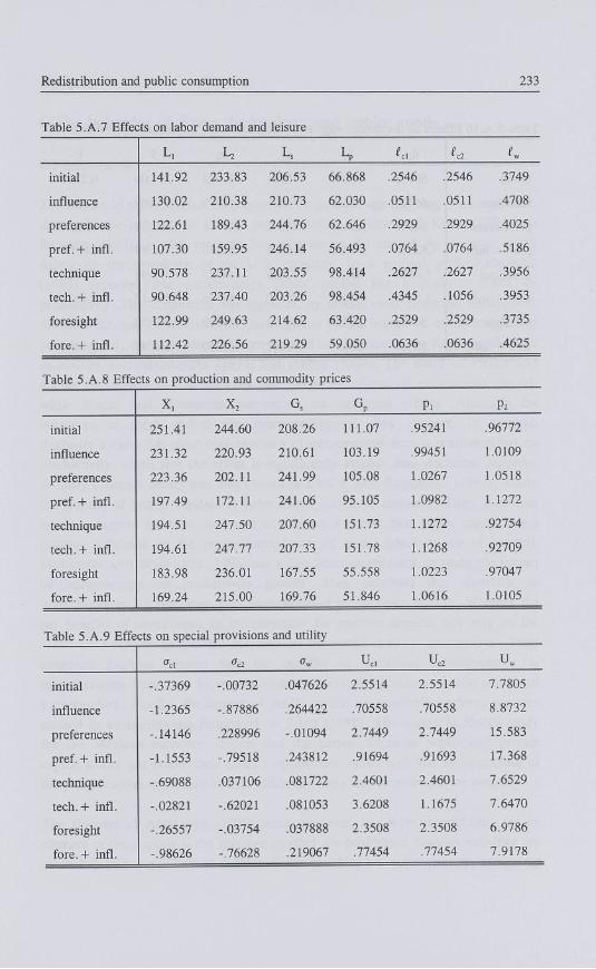
Redistribution and public consumption 233

Table 5.A.7 Effects on labor demand and leisure

L, U Ls Lp ' e l z* L

initial 141.92 233.83 206.53 66.868 .2546 .2546 .3749

influence 130.02 210.38 210.73 62.030 .0511 .0511 .4708

preferences 122.61 189.43 244.76 62.646 .2929 .2929 .4025

pref. + infl. 107.30 159.95 246.14 56.493 .0764 .0764 .5186

technique 90.578 237.11 203.55 98.414 .2627 .2627 .3956

tech. + infl. 90.648 237.40 203.26 98.454 .4345 .1056 .3953

foresight 122.99 249.63 214.62 63.420 .2529 .2529 .3735

fore.+ infl. 112.42 226.56 219.29 59.050 .0636 .0636 .4625

Table 5.A.8 Effects on production and commodity prices

x, X2 Gs Gp Pi P2

initial 251.41 244.60 208.26 111.07 .95241 .96772

influence 231.32 220.93 210.61 103.19 .99451 1.0109

preferences 223.36 202.11 241.99 105.08 1.0267 1.0518

pref. + infl. 197.49 172.11 241.06 95.105 1.0982 1.1272

technique 194.51 247.50 207.60 151.73 1.1272 .92754

tech.+ infl. 194.61 247.77 207.33 151.78 1.1268 .92709

foresight 183.98 236.01 167.55 55.558 1.0223 .97047

fore.+ infl. 169.24 215.00 169.76 51.846 1.0616 1.0105

Table 5.A.9 Effects on special provisions and utility

» c l "a ffw ucl uc2 uw

initial -.37369 -.00732 .047626 2.5514 2.5514 7.7805

influence -1.2365 -.87886 .264422 .70558 .70558 8.8732

preferences -.14146 .228996 -.01094 2.7449 2.7449 15.583

pref. + infl. -1.1553 -.79518 .243812 .91694 .91693 17.368

technique -.69088 .037106 .081722 2.4601 2.4601 7.6529

tech.+ infl. -.02821 -.62021 .081053 3.6208 1.1675 7.6470

foresight -.26557 -.03754 .037888 2.3508 2.3508 6.9786

fore.+ infl. -.98626 -.76628 .219067 .77454 .77454 7.9178

234 Chapter 5

Table 5.A. 10 Effects on dividends, wage rate, taxes and value of political interest function

d, d2 PL Th T P

initial .69438 .32801 .75924 .41002 244.00 6.2253

influence .66715 .30949 .79621 .43370 254.09 8.0857

preferences .66502 .29457 .84162 .48718 300.74 11.011

pref. + infl. .62870 .26882 .90964 .52370 318.49 14.993

technique 1.0461 .31812 .72615 .44383 263.48 6.0989

tech.+ infl. 1.0434 .31830 .72570 .44336 263.12 6.2935

foresight .54541 .31738 .68813 .36989 197.52 5.6138

fore. + infl. .52104 .30107 .71922 .39240 206.48 7.0490

Documents

UvA-DARE (Digital Academic Repository) Government ... · Government decisions on income redistribution and ... The more general characte of th modee r l presente in thd previoue s