Pervasive and Mobile Computing 13 (2014) 150–163

Contents lists available at ScienceDirect

Pervasive and Mobile Computing

journal homepage: www.elsevier.com/locate/pmc

Utilizing correlated node mobility for efficient DTN routing

Eyuphan Bulut a,b,∗, Sahin Cem Geyik a, Boleslaw K. Szymanski a,ca Rensselaer Polytechnic Institute, 110 8th St, Troy, NY 12180, United Statesb Cisco Systems, 2200 President George Bush Highway, Richardson, TX 75082, United Statesc Społeczna Akademia Nauk ul Sienkiewicza 9, 90-113 Łódź, Poland

a r t i c l e i n f o

Article history:Received 28 November 2012Received in revised form 14 September2013Accepted 20 September 2013Available online 30 September 2013

Keywords:Delay tolerant networksRoutingEfficiencyTemporal correlation

a b s t r a c t

In a delay tolerant network (DTN), nodes are connected intermittently and the futurenode connections are mostly not known. Therefore, effective forwarding based on limitedknowledge of contact behavior of nodes is challenging. Most of the previous studiesassumed thatmobility of a node is independent frommobility of other nodes and looked atonly the pairwise node relations to decide routing. In contrast, in this paper, we analyze thetemporal correlation between the meetings of each node with other nodes and utilize thiscorrelation for efficient routing. We introduce a newmetric called conditional intermeetingtime (CIT), which computes the average intermeeting time between two nodes relative toa meeting with a third node. Then, we modify existing DTN routing protocols using theproposed metric to improve their performance. Extensive simulations based on real andsynthetic DTN traces show that the modified algorithms perform better than the originalones.

© 2013 Elsevier B.V. All rights reserved.

1. Introduction

Delay tolerant networks (DTN) are wireless networks in which at any given time instance, the probability that there is anend-to-end path from a source to a destination is low due to the high mobility and low density of the nodes in the network.Routing of messages in such a challenging DTN environment is achieved opportunistically by utilizing the store-carry-and-forward paradigm at each node. Several DTN routing algorithms based on this paradigm have been proposed recently. Ineach, different techniques (single-copy [1–5], multi-copy [6–8], erasure coding [9,10]) with slightly different goals havebeen utilized. A survey of DTN routing algorithms can be found in [11].

Since DTNs consist of mobile agents that contact intermittently, recent studies on DTN routing have focused on theanalysis of real mobility traces (human [12], vehicular [13] etc.) and utilized extracted characteristics of the mobile objectsin the design of forwarding algorithms for DTNs.

Reviewing these designs and analyses, we have made the following observations. First, the future meetings of nodescan be predicted from their past relations using some distribution functions (e.g. log-normal [14,15]). Second, most ofthe previous routing protocols assume that meetings of a node with other nodes are independent from each other. Somealgorithms (e.g. Bubblerap [16]) implicitly consider the dependency between the node meetings thanks to their designswhich use real traces, however, there is no analysis and explicit usage of temporal correlation between the meetings of twonodes with a third node. Third, the mobility of many real objects are non-deterministic but periodic [17]. For example, in

∗ Corresponding author at: Rensselaer Polytechnic Institute, 110 8th St, Troy, NY 12180, United States. Tel.: +1 4694225653.E-mail addresses: ebulut@cisco.com, bulute@cs.rpi.edu (E. Bulut), geyiks@cs.rpi.edu (S.C. Geyik), szymansk@cs.rpi.edu (B.K. Szymanski).

1574-1192/$ – see front matter© 2013 Elsevier B.V. All rights reserved.http://dx.doi.org/10.1016/j.pmcj.2013.09.007

E. Bulut et al. / Pervasive and Mobile Computing 13 (2014) 150–163 151

a cyclic MobiSpace, if two nodes were frequently in contact at a particular time in previous cycles, then they are likely tomeet around the same time in the next cycle.

The above observations motivated us to study temporal correlation between the node meetings for designing moreefficient routing algorithms. Hence, we introduce a new link metric, conditional intermeeting time (CIT), that computes theaverage intermeeting time between two nodes relative to a meeting with a third node using only local knowledge of thepast contacts. Note that this definitionmakesmore sense in the context of routing because it refers to message holding timeon a given node during message routing.

We analyze CIT and discuss when and why it is beneficial in providing accurate information to nodes making routingdecisions. Different than our initial work [18], we also present statistical results from four different data sets (RollerNet [15],Cambridge [19], Haggle [20], MIT [21]) which contain the contact traces of real objects logged during real life experiments.

We then propose modifications to the existing DTN routing protocols using the proposed metric and demonstrate howtheir performance improves as the result. First, for the algorithms which route messages over shortest paths (SP) [22,23],we propose to use CIT rather than standard intermeeting times (SIT) and route the messages over conditional shortestpaths (CSP). Second, for the algorithms which make message forwarding decisions depending on a delivery metric (we callthemmetric-based forwarding algorithms), we propose to use CIT as a secondary delivery metric and allow the forwardingof messages if and only if both the algorithm’s original delivery metric and CIT agree to forward the message to theencountered node. Through simulations, we show the benefit of the proposed approach. In this extended version, we addednew simulation results and comparisons over our initial work [18]. In addition to real DTN traces, we also utilized syntheticand large-scale traces for simulations. Moreover, we added new results showing the superiority of the proposed approachover other popular algorithms (i.e., SimBet and CREST) and added new graphs showing the effects of some importantparameters (buffer space at nodes, message generation interval, and total node count) on the results.

The remainder of the paper is organized as follows. In Section 2, we describe the proposed metric (CIT) in detail and inSection 3, we provide its analysis. In Section 4, we describe how it can be used tomodify existing DTN routing algorithms forperformance improvement. In Section 5, we present simulation results. Finally, we offer conclusions and outline the futurework in Section 6.

2. Conditional intermeeting time

Recently, the research community working on routing algorithms in DTNs has focused on the analysis of real mobilitytraces to understand the main characteristics of mobile objects. Several experiments in different environments (office [14],conference [20], city [19], skating tour [15]) with different objects (human [12], bus [13]) and with variable number ofattendants were performed. From the analysis of the data sets collected during these experiments, significant results aboutthe aggregate and pairwise mobility characteristics of real objects were obtained and different kinds of algorithms usingdifferentmetrics developed for efficient routing ofmessages in DTNs. For example, in SimBet [24], a joint utilitymetric basedon social similarity and egocentric betweenness of nodes is used. In BubbleRap [16] two rankings (global and local) is usedto compute each node’s popularity (i.e., connectivity) in the local community and the entire society. Routing ofmessages arethen performed via nodes with high utility values. Moreover, in LocalCom [25], a community-based epidemic forwardingscheme,which first detects the community structure of the network and forwards themessages to each community throughgateways, is proposed.

Even though the previous studies modeled the node relations (i.e., intermeeting times) using different distributions(exponential [7,26], log-normal [15]) and developed their routing metrics accordingly, they assumed that the meetings of anodewith other nodes is independent of each other. The futuremeetings of two nodes are predicted looking at themeetingsof only these two nodes in the past. In [14], one additional attribute (the time passed since the lastmeeting) is also taken intoaccount formore accurate prediction. However, as we showwith statistics from real DTN traces, themeetings of a nodewithother nodesmay not be independent from each other (i.e., meetings are correlated), thus, prediction of future node relationscan be further improved with the analysis of temporal correlation between node meetings. In [5], each node establishes acommunity of nodes with whom it frequently meets to use for routing decisions when this node meets a message carrier.In contrast, in this paper, we consider a sequence of meetings of two specific nodes and use the statistics about subsequentmeetings of those nodes with the destination to make routing decisions.

We introduce a new metric called conditional intermeeting time (CIT), to define the node relations more precisely withinthe context of routing. This metric computes the average intermeeting time between two nodes relative to a meeting withan intermediate node using only the local knowledge of the past contacts.

The proposed metric can provide higher accuracy of prediction of delivery time, especially if the nodes move in a cyclicMobiSpace [17]. According to the definition of a cyclic MobiSpace, if two nodes contacted frequently at a particular timein previous cycles, the probability that they will be in contact around the same time in the next cycle is high. In Fig. 1, asample cyclic MobiSpace with three objects is illustrated. The fully repeating motion cycle is 12 time units. In this example,the discrete probabilistic contacts between A andM happen every 12 time units (1, 13, 25 . . .) and the discrete probabilisticcontacts between A and B occur every 6 time units (2, 8, 14 . . .). When we consider the intermeeting time between nodesA and B, we can expect that node Awill forward its message to node B in 3 time units (since a message can arrive at A at anytime within 6 s), however CIT of Awith B based on the condition that it has met (received the message from) nodeM let usknow that the message will be forwarded to node Bwithin 1 time unit.

152 E. Bulut et al. / Pervasive and Mobile Computing 13 (2014) 150–163

Fig. 1. An example cyclic MobiSpace with a common motion cycle of 12 time units.

Algorithm 1 updateSIT (nodem, time t)1: ifm is seen first time then2: firstTimeAt[m]← t3: else4: increment βm by 15: lastTimeAt[m]← t6: end if7: for each neighbor i ∈ N do8: τs(i)← (lastTimeAt[i] – firstTimeAt[i] ) / βi9: end for

Each node in a DTN can compute its SIT and CIT with other nodes using its contact history. In Algorithm 1, we showhow a node, s, can compute these metrics from previous node meetings. The notations we use in this algorithm (and alsothroughout the paper) are listed below with their meanings:

• τA(B|M): Average time it takes for node A to meet node B after meeting with node M . If B = M , the notation (in shortτA(B)) shows the standard intermeeting time (SIT) between nodes A and B.• S: N × N matrix where S (i, j) is the sum of all samples of conditional intermeeting times with node j relative to the

meeting with node i. Here, N is the neighbor count of current node (i.e., N(s) for node s).• C: N×N matrix where C (i, j) is the number of all conditional intermeeting time samples with node j relative to meeting

with node i.• βi: Total number of meetings with node i.

Algorithm 2 updateCIT (nodem, time t)1: for each neighbor j ∈ N and j =m do2: start a timer tmj3: end for4: for each neighbor j ∈ N and j =m do5: for each timer tjm running do6: S[j][m] += time on tjm7: increment C[j][m] by 18: end for9: if S[j][m] = 0 then

10: τs(m|j)← S[j][m] / C[j][m]11: end if12: delete all timers tjm13: end for

To find the CIT τA(B|M), each time node A meets node M , it starts a different timer for B. When it meets node B, it sumsup the values of these timers before deleting them. The value of τA(B|M) is then calculated by dividing the current total ofcollected timer values by the number of timers used so far. In Algorithm 2, we explain this procedure. Note that when thenode meets any node m, a timer is started for every other possible node (lines 1–3). Since meeting with node m will alsoend the conditional meeting time process for some other nodes, the corresponding timers whose clock has started at themeeting with other nodes but is scheduled to end at the meeting withm stop and their values are recorded (lines 4–8). CITvalues are then updated for all possible cases and the timers are deleted (lines 9–12). We can also use a sliding windowwithan appropriate size over the past contacts [23] and take into account the edge effects [13] to make the computation morelocal and current. Moreover, we do not consider the contact durations in these computations since inter-contact times are

E. Bulut et al. / Pervasive and Mobile Computing 13 (2014) 150–163 153

Fig. 2. Example meeting times of node Awith nodes B andM . Upper and lower values are used to compute τA(B|M) and τA(M|B), respectively.

usually much longer than contact times in real DTNs. However, if the last assumption does not hold, it is easy to modify allcomputations accordingly.

Consider the sample meeting times of a node A with its neighbors B and M in Fig. 2. Node A meets with node B attimes {5, 16, 25, 30} and with node M at times {11, 14, 23, 34}. Following the procedure described above, we find thatτA(B|M) = (5+ 2+ 2)/3 = 3 time units and τA(M|B) = (6+ 7+ 4+ 9)/4 = 6.5 time units while τA(B) = 8.33 time unitsand τA(M) = 7.67 time units.

3. Analysis

In this section, we give the analysis of CIT and showwhy it is significant in accurate prediction of future meetings withinthe context of routing.

Assume that node A has two different contacts, B andM , and assume that the intermeeting time of node AwithM is wellrepresented by a random variable XAM with the CDF DAM(x) and pdf dAM(x) = D′AM(x).

Then, let XAB|M denote the random variable representing the CIT of Awith B under the condition that it has metM beforemeeting B, with CDF DAB|M(x) and pdf dAB|M(x). Let also X t

(AM)B denote the random variable of time between the currentmeeting of A with M and the next meeting of A with B, with CDF Dt

(AM)B(x) and pdf dt(AM)B(x) given that t time units haspassed since the last meeting of Awith B and the current meeting of A and M . Then:

τA(B|M) =

∞

t=0dt(AM)BE[X

t(AM)B]dt.

In general, we can write in the case of such a meeting of A and M:

XAB|M = t + X t(AM)B.

Here, if A–M meeting is independent of A–Bmeeting, meaning that DAB|M = DAB, then:

Dt(AM)B(x) =

DAB(x+ t)− DAB(t)1− DAB(t)

dt(AM)B(x) =dAB(x+ t)1− DAB(t)

.

Hence:

E[X t(AM)B] =

∞

x=0 xdAB(t + x)dx1− DAB(t)

.

Then, using [z(1− D(z))]′ = 1− D(z)− zD′(z), we get:

E[X t(AM)B] =

∞

z=t(1− DAB(z))dz1− DAB(t)

.

There have been several distribution functions studied in previous work to model the pairwise intermeeting times.Using a distribution fitting software (EasyFit [27]), we also checked the fitness of several distribution functions includingexponential, Pareto and log-normal distribution and observed that intermeeting time (i.e., XAB) between nodes fits wellwith log-normal distribution. The analysis here can be updated for other distribution functions and is orthogonal to thedistribution function assumed. In case of log-normal distribution, we get:

E[X t(AM)B] = eµ+ σ2

2

1− erf

ln t−(µ+σ 2)

σ√2

1− erf

ln t−µ

σ√2

− t

where erf is the error function and µ and σ are mean and variance of XAB, respectively.Thus, if meeting of A with M is not correlated with meeting of A with B, E[X t

(AM)B] depends on t . However, consideringthe behavior of people in real life, temporal correlations often arise between A’s meetings with M and B (so A–B meeting

154 E. Bulut et al. / Pervasive and Mobile Computing 13 (2014) 150–163

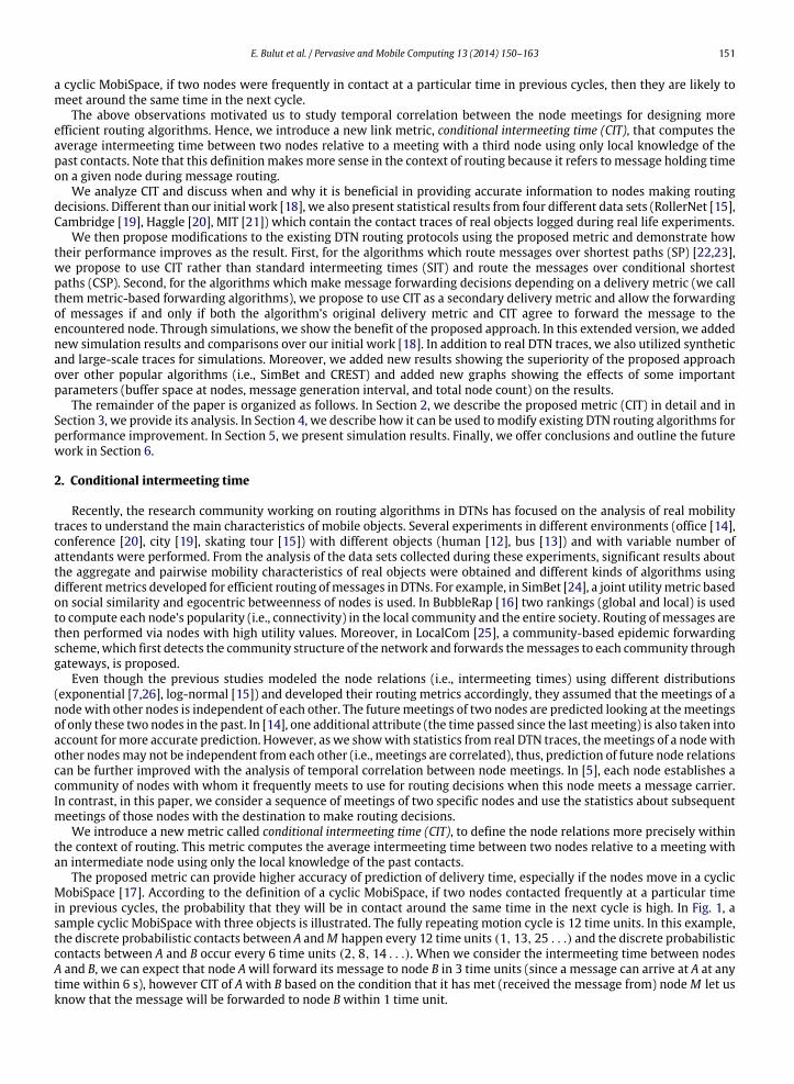
Fig. 3. Weighted average of relative standard deviation (RSD) for SIT and CIT in different datasets.

after AmetM depends on A–M meeting time), yielding a different dt(AM)B than it is in the uncorrelated case. This is the case,for example, when after AmeetsM , another stage of A’s journey starts and the length of this stage is largely independent ofwhat happened earlier. Consider meetings of a man who every morning goes from home to work. After meeting his familymembers (while leaving home), he meets later his office peers. Yet, on the way to his office, he meets the security guard atthe gate of his workplace a few moments before meeting his office peers. In other words, the meetings of this man with hisoffice peers are defined by the time when hemet the guard but independent of how long it took him tomeet the guard afterleaving home. E.g, if the trip from the gate to the office is normally distributed with the average and variance of 1 time unit,then X t

(AM)B ≈ N(1, 1) is independent of t , the travel time of the man from home to the gate. Therefore, we compute anduse the average of the time passed from A–M meeting to A–Bmeeting based on currently collected samples from encounterhistory.

Next, we present some statistics from available real DTN traces to show (i) the advantage of CIT over SIT and (ii) temporalcorrelation between the meetings of nodes.

For the first one, we found the answer to the question ‘What would the average error in predicting the future meetingsbe if the nodes could know their τA(B) and τA(B|M) values in advance?’. In SIT, for a given (A, B), this refers to standarddeviation (std) of SIT instances from their mean which is τA(B). Similarly, in CIT, for a given (A,M, B) tuple, this refers tostandard deviation (std) of CIT instances from their mean which is τA(B|M). However, to compute the average of this errorfor all possible and different (A, B) (in SIT) and (A,M, B) (in CIT) tuples, we computed the ‘relative standard deviation (RSD)’,computed as std/mean, and took theweighted average (WA) of these RSD values.More formally,WA-RSD for SIT is computedas follows:

WA-RSD(SIT) =

∀A=B

std(A,B)τA(B) |τA(B)|

∀A=B|τA(B)|

where |τA(B)| denotes the instance counts used in computing the τA(B) and std(A, B) denotes the standard deviation of theseinstances.

Similarly, for CIT, WA-RSD is computed as:

WA-RSD(CIT) =

∀A=M=B

std(A,M,B)τA(B|M)

|τA(B|M)|

∀A=M=B

|τA(B|M)|

.

To make these results statistically reliable, we only considered corresponding tuples with instance counts higher thana threshold and looked at the change in their value for different thresholds as well. Fig. 3 shows these results for different

E. Bulut et al. / Pervasive and Mobile Computing 13 (2014) 150–163 155

Table 1Ratio of all (A, B) pairs whose CIT values (τA(B|Mi)) for differentMis pass theANOVA test.

Instance count threshold Haggle RollerNet Cambridge MIT

10 96% 51% 64% 56%20 95% 42% 58% 54%

thresholds in four different datasets. Clearly, WA-RSD values of the CIT metric are smaller than WA-RSD values of the SITmetric in each dataset. Only for RollerNet traces [15], the results get closer for some thresholds. Consequently, these resultsshow that the CIT metric can provide more accurate prediction than the SIT metric for different environments.

To measure the temporal correlation between the meetings of nodes, we compare τA(B|M) values for different M ’s. Asthe above analysis shows, if A’s meetings withM are random, then E[X t

(AM)B] so the τA(B|M) should be the same for differentM ’s. To check if this is the case, we applied the ANOVA test on the CIT values of different M values. For each (A, B) pair, wefound τA(B|M0), τA(B|M1), . . . τA(B|Mk) values (and also all the instance values used to compute each mean τA(B|Mi)) for allapplicable Mi values (0 ≤ i ≤ k). Then, we applied the ANOVA test to learn whether these τA(B|Mi) values and also theirinstance value distribution differ from each other significantly (with α = 0.05) for given pair (A, B). Table 1 shows the ratioof all (A, B) pairs which pass this ANOVA test in different datasets. Clearly, the results indicate that for a remarkable amountof (A, B) pairs, CIT values computed using different M values are significantly different from each other. This indicates thatthe identity of met intermediate node (M) is significant (in predicting the A’s future meeting with B) for all datasets. Thus,there is a temporal correlation between the meetings of a node with other nodes. If there were no such correlation, τA(B|M)would have been the same (or close) for different M ’s for given pair (A, B), causing the failure in ANOVA tests. In contrast,we observe that these values are significantly different from each other.1

4. Proposed algorithms

In this section, we present two different applications of CIT to the existing DTN routing algorithms. First, we look intothe shortest path based routing algorithms and propose to use conditional shortest paths to route messages. Second, wepropose to revise message forwarding decisions of metric-based forwarding algorithms by including CIT.

4.1. Shortest path based routing

4.1.1. OverviewShortest path routing (SPR) protocols for DTNs are based on the designs of routing protocols for traditional networks. The

links between each pair of nodes are assigned a cost andmessages are forwarded over the shortest paths between the sourceand the destination. Furthermore, the dynamic nature of DTNs is also addressed in these designs. Two of the commonmetricsused to define the link cost are minimum expected delay (MED [22]) and minimum estimated expected delay (MEED [23]).These metrics compute the expected waiting time plus the transmission delay between each pair of nodes. However, whilethe former uses the future contact schedule, the latter uses only observed contact history.

In SPR, a routing decision can be made: (i) at source node, (ii) at each hop, and (iii) at each contact with other nodes.The utilization of recent contact information increases from the first to the last one improving the quality of the forwardingdecisions; however, more processing resources are used as the routing decisions are made more frequently.

The suitability of SPR algorithms for DTNs and the scalability and complexity of their designs have been already discussedin [22,23], hence, in this paper, we focus on the enhancements of the performance of SPR algorithms achieved by utilizingour metric (CIT), rather than using SIT. To this end, in the rest of this section, we show the necessary changes to the currentdesigns of SPR algorithms.

4.1.2. Network modelWe model a DTN as a graph G = (V ′, E ′) where the mobile nodes are represented by vertices (V ′) and the possible

connections between these nodes are represented by the edges. Unlike previous DTN graph models, since CIT considersnode relations with respect to a third node, we define V ′ and E ′ sets in a different way. Given V is the set of all node namesand N(i) denotes the set of other nodes that meet with node i (i.e. neighbors of node i):

V ⊆ V × V and E ′ ⊆ V ′ × V ′ where,V ′ = {(ij) | ∀j ∈ N(i)}E ′ = {(ij, kl) | i = l}

where, w′(ij, kl) =τi(k|j) if j = kτi(k) otherwise.

1 It might also be interesting to analyze the divergence of ANOVA test results in different datasets and its impact on simulation results, which we willstudy in our future work.

156 E. Bulut et al. / Pervasive and Mobile Computing 13 (2014) 150–163

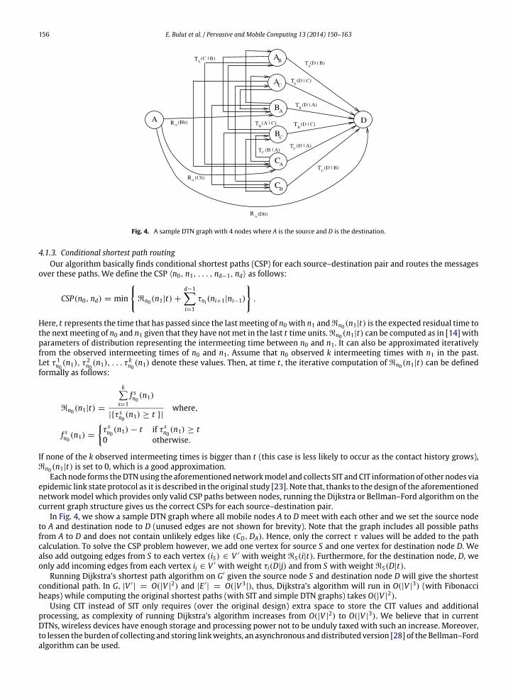
Fig. 4. A sample DTN graph with 4 nodes where A is the source and D is the destination.

4.1.3. Conditional shortest path routingOur algorithm basically finds conditional shortest paths (CSP) for each source–destination pair and routes the messages

over these paths. We define the CSP ⟨n0, n1, . . . , nd−1, nd⟩ as follows:

CSP(n0, nd) = min

ℜn0(n1|t)+

d−1i=1

τni(ni+1|ni−1)

.

Here, t represents the time that has passed since the lastmeeting of n0 with n1 andℜn0(n1|t) is the expected residual time tothe nextmeeting of n0 and n1 given that they have notmet in the last t time units.ℜn0(n1|t) can be computed as in [14] withparameters of distribution representing the intermeeting time between n0 and n1. It can also be approximated iterativelyfrom the observed intermeeting times of n0 and n1. Assume that n0 observed k intermeeting times with n1 in the past.Let τ 1

n0(n1), τ2n0(n1), . . . τ

kn0(n1) denote these values. Then, at time t , the iterative computation of ℜn0(n1|t) can be defined

formally as follows:

ℜn0(n1|t) =

ks=1

f sn0(n1)

|{τ sn0(n1) ≥ t }|

where,

f sn0(n1) =

τ sn0(n1)− t if τ s

n0(n1) ≥ t0 otherwise.

If none of the k observed intermeeting times is bigger than t (this case is less likely to occur as the contact history grows),ℜn0(n1|t) is set to 0, which is a good approximation.

Eachnode forms theDTNusing the aforementionednetworkmodel and collects SIT andCIT information of other nodes viaepidemic link state protocol as it is described in the original study [23]. Note that, thanks to the design of the aforementionednetworkmodel which provides only valid CSP paths between nodes, running the Dijkstra or Bellman–Ford algorithm on thecurrent graph structure gives us the correct CSPs for each source–destination pair.

In Fig. 4, we show a sample DTN graph where all mobile nodes A to D meet with each other and we set the source nodeto A and destination node to D (unused edges are not shown for brevity). Note that the graph includes all possible pathsfrom A to D and does not contain unlikely edges like (CD,DA). Hence, only the correct τ values will be added to the pathcalculation. To solve the CSP problem however, we add one vertex for source S and one vertex for destination node D. Wealso add outgoing edges from S to each vertex (iS) ∈ V ′ with weight ℜS(i|t). Furthermore, for the destination node, D, weonly add incoming edges from each vertex ij ∈ V ′ with weight τi(D|j) and from S with weightℜS(D|t).

Running Dijkstra’s shortest path algorithm on G′ given the source node S and destination node D will give the shortestconditional path. In G, |V ′| = O(|V |2) and |E ′| = O(|V 3

|), thus, Dijkstra’s algorithm will run in O(|V |3) (with Fibonacciheaps) while computing the original shortest paths (with SIT and simple DTN graphs) takes O(|V |2).

Using CIT instead of SIT only requires (over the original design) extra space to store the CIT values and additionalprocessing, as complexity of running Dijkstra’s algorithm increases from O(|V |2) to O(|V |3). We believe that in currentDTNs, wireless devices have enough storage and processing power not to be unduly taxed with such an increase. Moreover,to lessen the burden of collecting and storing linkweights, an asynchronous and distributed version [28] of the Bellman–Fordalgorithm can be used.

E. Bulut et al. / Pervasive and Mobile Computing 13 (2014) 150–163 157

4.1.4. Why CSPR offers better performance?The difference between CSPR and SPR path definitions is that CSPR defines the link weights based on the previous node

while SPR does not. In SPR, the path (SP) can be defined as:

SP(n0, nd) = min

ℜn0(n1|t)+

d−1i=1

τni(ni+1)

2

.

After the first hop, since the message can reach the nodes at any time between their interaction with other nodes, eachlink weight can be approximated as

τni (ni+1)2 . However, the link weight can better be defined via τni(ni+1|ni−1). If there is no

temporal correlation between, say, n1’s meetings with n0 and n2, then τn1(n2|n0) converges toτn1 (n2)

2 , but if such correctionexists (which is often the case as shown in statistics from real DTN traces) then these values will be different and routingvia CSPR will therefore be faster.2

4.2. Metric-based forwarding algorithms

4.2.1. OverviewA commonmethod of routing in DTNs is to forward themessage to the encountered node that is more likely tomeet with

destination than the current message carrier. However, making effective forwarding decisions in single-copy based routingin DTNs is a challenging task. When two nodes meet, one of them forwards a message to the other one if it decides that themessage will have a higher chance to be delivered to the destination at the other node.

In previouswork, depending on the observed contact history between nodes, severalmetrics have been used to define thedelivery quality of nodes. Popular ones include encounter frequency [2], time elapsed since last encounter [29,30], residualtime [14] and social similarity [24,16].

4.2.2. Proposed modificationIn most of the previous work, meetings of a node with other nodes are assumed independent from each other and the

forwarding decision at the encounter of two nodes is made depending on their individual relations with the destinationnode. In some algorithms such as [2,30], with additional processing (i.e. applying transitivity) on pairwise meetings, moreaccuratemetrics are used to reflect the effect of other nodes on the delivery quality of a node. However, these improvementscan also be applied to all other metrics, including the one introduced in this paper. Our contribution is the introduction of anew metric having this property by default in its basic definition.

To make forwarding decisions of these algorithms more effective, thus to improve their performance, we propose touse CIT as an additional delivery metric. That is, when two nodes meet, they will also compare their CIT with destination(depending on the condition that they met each other). If the current carrier of the message learns that the other node alsohas a shorter remaining time (according to CIT) tomeet the destination than itself, themessage is forwarded. This additionalcondition eliminates forwardings that based on CIT became harmful and if executedwould decrease the delivery probability.Simulation results confirm this conclusion, as the delivery rates are preserved and simply unbeneficial forwardings are notperformed. Therefore, more effective forwarding decisions are made so that the cost of message delivery declines whilethe delivery ratio and average delay are maintained (in some cases, even the delivery ratio increases and average delaydecreases).

4.2.3. Why modification offers better performance?With the addition of CIT as the second forwarding condition, forwarding decisions are made depending on both the

pairwise node relations between A and B (due to themetric of the original algorithm) and also possible temporal correlationsbetween the meetings of A with nodes M and B. If there is no such correlation, CIT often supports the forwarding if theoriginal metric also supports the forwarding. However, when this correlation is strong, CIT offers more accurate predictionand it may indicate that at the time of the meeting the forwarding is no longer beneficial. Thus, the statistically harmfulforwarding decisions without considering possible correlations are prevented. Even though addition of CIT makes modifiedalgorithms more selective, the messages are forwarded to or stay with the nodes which have higher delivery probability atthe time of the meeting with nodeM .3 Thus, delivery performance stays similar or improves while the cost (i.e., the numberof forwardings) decreases, yielding better routing efficiency.

2 It is should be noted that the values of the τ function are approximated iteratively. However they are used to select the minimum delay paths, so theerror of selection is bounded by the error of approximation. In other words, if iterative averages are close to each other, so are the real averages, thus wrongselection will have a small impact on performance. Moreover, such an error of selection arises in all routing methods using the iteratively approximatedaverages. Thus, this error does not negate the improvements of CSPR.3 Note that the path to delivery in modified algorithms can be totally different than the path in original algorithms. In the original algorithm A may

forward the message to M1 but in the modified version, A may skip M1 due to the unsatisfied CIT condition and later forward the message to M2 whichsatisfies both conditions. The remaining paths of the message towards the destination in both cases are likely to continue to be partially disjoint.

158 E. Bulut et al. / Pervasive and Mobile Computing 13 (2014) 150–163

5. Performance evaluation

To evaluate the performance of proposed algorithms, we have built a Java based custom DTN simulator. It uses eitherthe traces of real objects from real DTN environments or the traces which are built synthetically. The network parameters(number of nodes etc.) are set according to the traces used.

5.1. Algorithms in comparison

We compared existing DTN algorithms with their CIT-usingmodified versions. First, we compared Shortest Path Routing(SPR) with Conditional Shortest Path Routing (CSPR) which is described in Section 4.1.3. Then, we compared the existingand revised versions of three metric-based DTN routing algorithms: Prophet [2], Fresh [29] and SimBet [24]. In the revisedversions of these algorithms (referred to as C-Prophet, C-Fresh and C-SimBet to underline that they use CIT), A forwards themessage to B if τA(D|B) > τB(D|A) is also satisfied (in addition to the algorithm’s own forwarding condition). In the graphs,we also give the results obtained by Epidemic Routing [6] since it achieves the optimum delivery ratio and delay (at highcost, however).

5.2. Datasets

For the main simulations, we used three real and one synthetic DTN traces. Real traces are from RollerNet [15],Cambridge [19] and Haggle [20] datasets where Bluetooth sightings between respectively 62, 36 and 41 user mobile devicesare recorded. Further details of these traces can be found in the crawdad archive [31]. Synthetic traces are generated usinga community-based mobility model which is similar to the models in [25,32,33]. In a 1000 units by 1000 units squareregion, we generated Nc randomly located non-overlapping community regions (home, work, school etc.) of size 100 unitsby 100 units and distributed Np nodes (i.e. people) to these community regions. For each node, we randomly assigned Vcommunities to visit (i.e. commonly visited places for a person in a day). Each node first selects a random point withinthe next community region in its list, assigns a random speed in range [Vmin, Vmax] and moves towards the target pointwith that speed. Once it reaches that point, it randomly assigns a visit duration in range [Tmin, Tmax] and randomly walkswithin the community region for that visit duration. Once that duration expires, it moves to the next community in itslist in a similar way. Each node visits all the communities in its list as indicated, then once all of them are done (i.e. theend of day), they again start the same process and start visiting the communities in their list. While nodes are moving, werecord themeetings between nodes assuming they have a transmission range of R. The default values for the parameters areNc = 10,Np = 50, V = 5, Vmin = 10 units, Vmax = 50 units, Tmin = 20 time units, Tmax = 50 time units. However, we alsolooked at the effects of different values of parameters in simulations. We also used large scale WiFi traces [34] to evaluatethe performance of the proposed approach in large scale networks.

5.3. Simulation results

To collect several routing statistics, we have generated traffic on the aforementioned traces. For each simulation run, afterawarm up period4 (20% of the data), we generated 5000messages from a random source node to a randomdestination nodeat each t seconds. In RollerNet, since the duration of the experiment is short, we set t = 1 s, but for Cambridge and Haggledatasets, we set t = 1 min and t = 30 s, respectively. For synthetic traces, we set t = 10 time units. Besides this singledifference, we compare all algorithms in the same conditions.

For main simulations, we assume that the nodes have enough buffer space to store every message they receive,5 thebandwidth is high and the contact durations of nodes are long enough to allow the exchange of all messages between nodes.These assumptions are reasonable in view of the capabilities of today’s technology and are also used commonly in previousstudies [35,26]. Any change in the current assumptions is expected to affect the performance of compared algorithms in thesame way since they use one copy of the message. Moreover, we used a simplified slotted CSMA MAC model as in [7]. Weran each simulation 10 times with different seeds and in each run, we collect statistics by running each algorithm on thesame set of messages. All results plotted in the figures show the averages of results obtained in all runs.

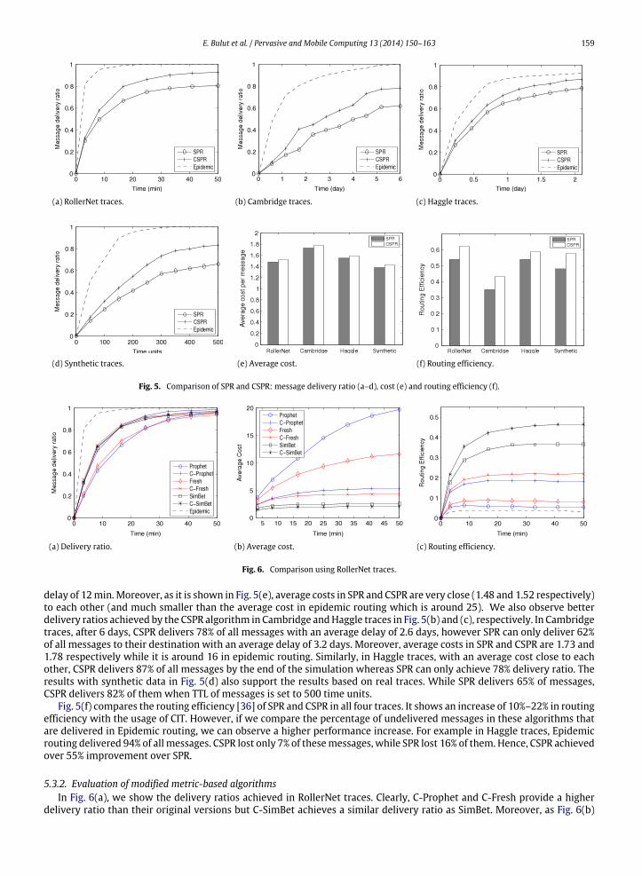
5.3.1. Comparison of CSPR and SPRFig. 5(a) shows6 the delivery ratios achieved in CSPR and SPR algorithms with respect to time (i.e., TTL of messages) in

RollerNet traces. Clearly, the CSPR algorithmdeliversmoremessages to their destinations than the SPR algorithm.Moreover,it achieves lower average delivery delay than the SPR algorithm. For example, CSPR delivers 80% of all messages after 17minwith an average delay of almost 6 min, while SPR achieves the same delivery ratio only after 41 min and with an average

4 During the warm up period, nodes build some encounter history to compute their initial CIT values. After the warm up period, as the messages arereceived and new meetings happen, CIT values are updated in parallel and the forwarding decisions are performed using the updated CIT values.5 The largest number ofmessages in a node buffer over all simulationswas 120messages, so in the order of 12Mb, well below the buffer space inmodern

wireless devices.6 Error bars are not shown since they are so small.

E. Bulut et al. / Pervasive and Mobile Computing 13 (2014) 150–163 159

(a) RollerNet traces. (b) Cambridge traces. (c) Haggle traces.

(d) Synthetic traces. (e) Average cost. (f) Routing efficiency.

Fig. 5. Comparison of SPR and CSPR: message delivery ratio (a–d), cost (e) and routing efficiency (f).

(a) Delivery ratio. (b) Average cost. (c) Routing efficiency.

Fig. 6. Comparison using RollerNet traces.

delay of 12min.Moreover, as it is shown in Fig. 5(e), average costs in SPR and CSPR are very close (1.48 and 1.52 respectively)to each other (and much smaller than the average cost in epidemic routing which is around 25). We also observe betterdelivery ratios achieved by the CSPR algorithm in Cambridge andHaggle traces in Fig. 5(b) and (c), respectively. In Cambridgetraces, after 6 days, CSPR delivers 78% of all messages with an average delay of 2.6 days, however SPR can only deliver 62%of all messages to their destination with an average delay of 3.2 days. Moreover, average costs in SPR and CSPR are 1.73 and1.78 respectively while it is around 16 in epidemic routing. Similarly, in Haggle traces, with an average cost close to eachother, CSPR delivers 87% of all messages by the end of the simulation whereas SPR can only achieve 78% delivery ratio. Theresults with synthetic data in Fig. 5(d) also support the results based on real traces. While SPR delivers 65% of messages,CSPR delivers 82% of them when TTL of messages is set to 500 time units.

Fig. 5(f) compares the routing efficiency [36] of SPR and CSPR in all four traces. It shows an increase of 10%–22% in routingefficiency with the usage of CIT. However, if we compare the percentage of undelivered messages in these algorithms thatare delivered in Epidemic routing, we can observe a higher performance increase. For example in Haggle traces, Epidemicrouting delivered 94% of all messages. CSPR lost only 7% of thesemessages, while SPR lost 16% of them. Hence, CSPR achievedover 55% improvement over SPR.

5.3.2. Evaluation of modified metric-based algorithmsIn Fig. 6(a), we show the delivery ratios achieved in RollerNet traces. Clearly, C-Prophet and C-Fresh provide a higher

delivery ratio than their original versions but C-SimBet achieves a similar delivery ratio as SimBet. Moreover, as Fig. 6(b)

160 E. Bulut et al. / Pervasive and Mobile Computing 13 (2014) 150–163

(a) Delivery ratio. (b) Average cost. (c) Routing efficiency.

Fig. 7. Comparison using Cambridge traces.

(a) Delivery ratio. (b) Average cost. (c) Routing efficiency.

Fig. 8. Comparison using Haggle traces.

(a) Delivery ratio. (b) Average cost. (c) Routing efficiency.

Fig. 9. Comparison using synthetic traces.

shows, average cost is lower for the modified algorithms. For example, C-Prophet delivers 90% of all messages after 23 minwith average delay of 7.8 min and average cost of 4.83 hops. However, the original Prophet reaches the same delivery ratioonly after 33 min with average delay of 13.5 min and average cost of 17.02. A similar situation is also observed betweenC-Fresh and Fresh, and C-SimBet and SimBet. As a result, over 100% increase in C-Prophet and C-Fresh, and around 30%increase in C-SimBet is achieved in routing efficiency (Fig. 6(c)).

When we look at the results obtained from Cambridge and Haggle traces in Figs. 7 and 8, we observe a differentimprovement. As it is seen in Figs. 7(a) and 8(a), revised and original versions of all algorithms have similar delivery ratios(and therefore similar average delays). However, as Figs. 7(b) and 8(b) show, average costs in modified versions are lowerthan they are in the original ones. This shows that when CIT is used as an additional delivery metric, the nodes choosebetter next hops so that the cost decreases while still keeping the original delivery ratio. Therefore, again the routingefficiency (Figs. 7(c) and 8(c)) is increased in all revised algorithms remarkably. The results with synthetic data in Fig. 9also demonstrate the superiority of the revised algorithms. More (in C-Prophet and C-Fresh) or at least the same number ofmessages (in C-SimBet) are delivered with lower cost when compared to the original algorithms. From the above results,we clearly observe the benefit of CIT in metric-based forwarding algorithms.

E. Bulut et al. / Pervasive and Mobile Computing 13 (2014) 150–163 161

(a) Effect of buffer space. (b) Effect of message generation interval. (c) Effect of node count.

Fig. 10. Extensive results.

(a) Improvement over CREST. (b) Results with WiFi traces.

Fig. 11. Results showing (a) the comparison with CREST and (b) the performance in WiFi traces.

5.3.3. Effects of simulation parameters on resultsWe evaluate here the impact of some parameters on the results. First, we look at the scenarios where the buffer

space at nodes is limited. Assuming that nodes use the FIFO buffer management scheme, we measured routing efficiencyimprovements delivered by the proposedmetric over the original algorithms. Fig. 10(a) shows the results for different buffersizes in the range of [15–100]messages (in Cambridge traces). For these simulationswe kept themessage generation intervalt = 1 min and TTL = 4 days. The results show that in the modified versions of algorithms, the increase in the routingefficiency grows as the buffer space increases. Moreover, the increase converges to a constant value after sufficient bufferspaces is allocated. CSPR, C-SimBet, C-Fresh, and C-Prophet offer 22%, 26% 48% and 130% increase in the routing efficiencyover their original algorithms, respectively.

In Fig. 10(b), we observe similar results with different message generation intervals. As the messages are generatedmore frequently, due to buffer overflow, some messages are lost. However, the routing efficiency of algorithms is stillremarkably increased with the modified versions. Finally, we changed the node count in the network (in synthetic traces)and looked at the effect of node count on results. Fig. 10(c) clearly shows that the increase in routing efficiency risesas the node count increases. This is because in synthetic data, temporal correlation between the meetings of nodesincreases due to the higher number of nodes in each community. Thus, CIT provides more accurate information about noderelations.

5.3.4. Comparison with closest related workEven though several DTN routing algorithms have been proposed in literature, they usually assume that the meetings of

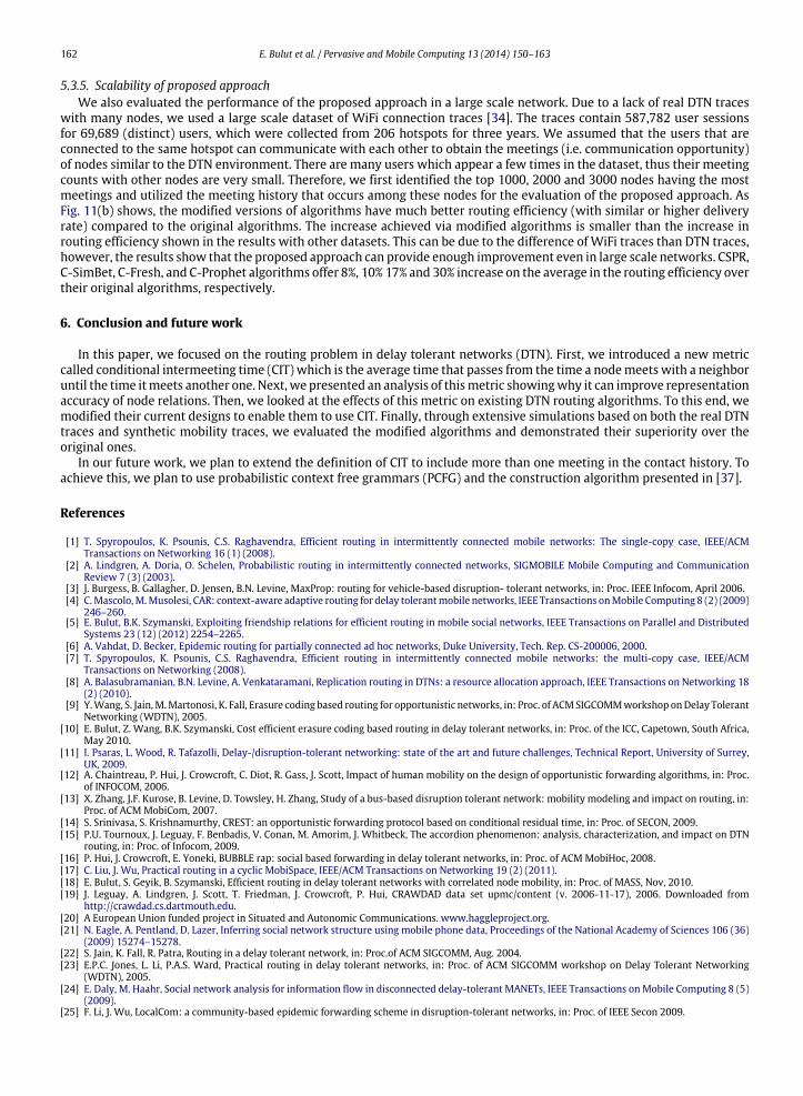
a node with other nodes are independent and identically distributed. The closest study to our work is in [14], where a newmetric, conditional residual time (CREST), which computes the remaining time for the meetings of two nodes based on thecondition that t time units has passed since their last encounter, is proposed. However, the relations with other nodes is stillnot considered in this computation and meetings of a node with other nodes are assumed independent. In case of temporalcorrelation between the meetings of a node with other nodes, CIT can predict the remaining time to the next meeting ofnodes more accurately, while CREST cannot differentiate the cases where two different nodes are met at the same elapsedtime since the last meeting with destination and yields less accurate prediction. Fig. 11(a) shows how much improvementCIT can achieve over CRESTwhilemaintaining (sometimes increasing) the delivery rate in all traces. The results clearly showthe superiority of CIT over CREST with an improvement in the range of 20%–37%.

162 E. Bulut et al. / Pervasive and Mobile Computing 13 (2014) 150–163

5.3.5. Scalability of proposed approachWe also evaluated the performance of the proposed approach in a large scale network. Due to a lack of real DTN traces

with many nodes, we used a large scale dataset of WiFi connection traces [34]. The traces contain 587,782 user sessionsfor 69,689 (distinct) users, which were collected from 206 hotspots for three years. We assumed that the users that areconnected to the same hotspot can communicate with each other to obtain the meetings (i.e. communication opportunity)of nodes similar to the DTN environment. There are many users which appear a few times in the dataset, thus their meetingcounts with other nodes are very small. Therefore, we first identified the top 1000, 2000 and 3000 nodes having the mostmeetings and utilized the meeting history that occurs among these nodes for the evaluation of the proposed approach. AsFig. 11(b) shows, the modified versions of algorithms have much better routing efficiency (with similar or higher deliveryrate) compared to the original algorithms. The increase achieved via modified algorithms is smaller than the increase inrouting efficiency shown in the results with other datasets. This can be due to the difference of WiFi traces than DTN traces,however, the results show that the proposed approach can provide enough improvement even in large scale networks. CSPR,C-SimBet, C-Fresh, and C-Prophet algorithms offer 8%, 10% 17% and 30% increase on the average in the routing efficiency overtheir original algorithms, respectively.

6. Conclusion and future work

In this paper, we focused on the routing problem in delay tolerant networks (DTN). First, we introduced a new metriccalled conditional intermeeting time (CIT) which is the average time that passes from the time a nodemeets with a neighboruntil the time itmeets another one. Next, we presented an analysis of thismetric showingwhy it can improve representationaccuracy of node relations. Then, we looked at the effects of this metric on existing DTN routing algorithms. To this end, wemodified their current designs to enable them to use CIT. Finally, through extensive simulations based on both the real DTNtraces and synthetic mobility traces, we evaluated the modified algorithms and demonstrated their superiority over theoriginal ones.

In our future work, we plan to extend the definition of CIT to include more than one meeting in the contact history. Toachieve this, we plan to use probabilistic context free grammars (PCFG) and the construction algorithm presented in [37].

References

[1] T. Spyropoulos, K. Psounis, C.S. Raghavendra, Efficient routing in intermittently connected mobile networks: The single-copy case, IEEE/ACMTransactions on Networking 16 (1) (2008).

[2] A. Lindgren, A. Doria, O. Schelen, Probabilistic routing in intermittently connected networks, SIGMOBILE Mobile Computing and CommunicationReview 7 (3) (2003).

[3] J. Burgess, B. Gallagher, D. Jensen, B.N. Levine, MaxProp: routing for vehicle-based disruption- tolerant networks, in: Proc. IEEE Infocom, April 2006.[4] C.Mascolo,M.Musolesi, CAR: context-aware adaptive routing for delay tolerantmobile networks, IEEE Transactions onMobile Computing 8 (2) (2009)

246–260.[5] E. Bulut, B.K. Szymanski, Exploiting friendship relations for efficient routing in mobile social networks, IEEE Transactions on Parallel and Distributed

Systems 23 (12) (2012) 2254–2265.[6] A. Vahdat, D. Becker, Epidemic routing for partially connected ad hoc networks, Duke University, Tech. Rep. CS-200006, 2000.[7] T. Spyropoulos, K. Psounis, C.S. Raghavendra, Efficient routing in intermittently connected mobile networks: the multi-copy case, IEEE/ACM

Transactions on Networking (2008).[8] A. Balasubramanian, B.N. Levine, A. Venkataramani, Replication routing in DTNs: a resource allocation approach, IEEE Transactions on Networking 18

(2) (2010).[9] Y.Wang, S. Jain,M.Martonosi, K. Fall, Erasure coding based routing for opportunistic networks, in: Proc. of ACMSIGCOMMworkshop onDelay Tolerant

Networking (WDTN), 2005.[10] E. Bulut, Z. Wang, B.K. Szymanski, Cost efficient erasure coding based routing in delay tolerant networks, in: Proc. of the ICC, Capetown, South Africa,

May 2010.[11] I. Psaras, L. Wood, R. Tafazolli, Delay-/disruption-tolerant networking: state of the art and future challenges, Technical Report, University of Surrey,

UK, 2009.[12] A. Chaintreau, P. Hui, J. Crowcroft, C. Diot, R. Gass, J. Scott, Impact of human mobility on the design of opportunistic forwarding algorithms, in: Proc.

of INFOCOM, 2006.[13] X. Zhang, J.F. Kurose, B. Levine, D. Towsley, H. Zhang, Study of a bus-based disruption tolerant network: mobility modeling and impact on routing, in:

Proc. of ACMMobiCom, 2007.[14] S. Srinivasa, S. Krishnamurthy, CREST: an opportunistic forwarding protocol based on conditional residual time, in: Proc. of SECON, 2009.[15] P.U. Tournoux, J. Leguay, F. Benbadis, V. Conan, M. Amorim, J. Whitbeck, The accordion phenomenon: analysis, characterization, and impact on DTN

routing, in: Proc. of Infocom, 2009.[16] P. Hui, J. Crowcroft, E. Yoneki, BUBBLE rap: social based forwarding in delay tolerant networks, in: Proc. of ACMMobiHoc, 2008.[17] C. Liu, J. Wu, Practical routing in a cyclic MobiSpace, IEEE/ACM Transactions on Networking 19 (2) (2011).[18] E. Bulut, S. Geyik, B. Szymanski, Efficient routing in delay tolerant networks with correlated node mobility, in: Proc. of MASS, Nov, 2010.[19] J. Leguay, A. Lindgren, J. Scott, T. Friedman, J. Crowcroft, P. Hui, CRAWDAD data set upmc/content (v. 2006-11-17), 2006. Downloaded from

http://crawdad.cs.dartmouth.edu.[20] A European Union funded project in Situated and Autonomic Communications. www.haggleproject.org.[21] N. Eagle, A. Pentland, D. Lazer, Inferring social network structure using mobile phone data, Proceedings of the National Academy of Sciences 106 (36)

(2009) 15274–15278.[22] S. Jain, K. Fall, R. Patra, Routing in a delay tolerant network, in: Proc.of ACM SIGCOMM, Aug. 2004.[23] E.P.C. Jones, L. Li, P.A.S. Ward, Practical routing in delay tolerant networks, in: Proc. of ACM SIGCOMM workshop on Delay Tolerant Networking

(WDTN), 2005.[24] E. Daly, M. Haahr, Social network analysis for information flow in disconnected delay-tolerant MANETs, IEEE Transactions on Mobile Computing 8 (5)

(2009).[25] F. Li, J. Wu, LocalCom: a community-based epidemic forwarding scheme in disruption-tolerant networks, in: Proc. of IEEE Secon 2009.

E. Bulut et al. / Pervasive and Mobile Computing 13 (2014) 150–163 163

[26] E. Bulut, Z. Wang, B. Szymanski, Cost-effective multi-period spraying for routing in delay tolerant networks, IEEE/ACM Transactions on Networking18 (5) (2010).

[27] EasyFit: distribution fitting software. http://www.mathwave.com/ (last accessed in August, 2013).[28] D. Bertsekas, R. Gallager, Data Networks, second ed., 1992.[29] H. Dubois-Ferriere, M. Grossglauser, M. Vetterli, Age matters: efficient route discovery in mobile ad hoc networks using encounter ages, in: Proc. of

ACMMobiHoc, 2003.[30] T. Spyropoulos, K. Psounis, C. Raghavendra, Spray and focus: efficient mobility-assisted routing for heterogeneous and correlated mobility, in: Proc.

of IEEE PerCom, 2007.[31] CRAWDAD data set. http://crawdad.cs.dartmouth.edu.[32] W. Hsu, T. Spyropoulos, K. Psounis, A. Helmy, Modeling time variant user mobility in wireless mobile networks, in: IEEE INFOCOM, 2007.[33] T. Spyropoulos, K. Psounis, C.S. Raghavendra, Performance analysis of mobility-assisted routing, in: Proc. of MobiHoc, 2006.[34] M. Lenczner, B. Grégoire, F. Proulx, CRAWDAD trace set ilesansfil/wifidog/session (v. 2007-08-27), 2013. Downloaded from

http://crawdad.cs.dartmouth.edu/ilesansfil/wifidog/session. July.[35] C. Liu, J. Wu, On multicopy opportunistic forwarding protocols in nondeterministic delay tolerant networks, IEEE Transactions on Parallel and

Distributed Systems 23 (6) (2012) 1121–1128.[36] J.M. Pujol, A.L. Toledo, P. Rodriguez, Fair routing in delay tolerant networks, in: Proc. of Infocom, 2009.[37] S. Geyik, E. Bulut, B. Szymanski, Grammatical inference for modeling mobility patterns in networks, IEEE Transactions on Mobile Computing (TMC)

12 (11) (2013) 2119–2131.