Embed Size (px)
Citation preview
Utilizing ASHRAE G36 for Free Outside Air Cooling (Economizer)
by Alejandro Rodriguez
B.A. in Construction Management, August 2014, National Labor College
M.S. in Construction Management, August 2016, Arizona State University
A Praxis submitted to
The Faculty of
The School of Engineering and Applied Science
of the George Washington University
in partial fulfillment of the requirements
for the degree of Doctor of Engineering
January 10, 2019
Praxis directed by
Timothy Blackburn
Professorial Lecturer of Engineering Management and Systems Engineering
ii
The School of Engineering and Applied Science of The George Washington University
certifies that Alejandro Rodriguez has passed the Final Examination for the degree of
Doctor of Engineering as of date of dissertation defense. This is the final and approved
form of the praxis.
Utilizing ASHRAE G36 for Free Outside Air Cooling (Economizer)
Alejandro Rodriguez
Dissertation Research Committee:
Timothy Blackburn, Professorial Lecturer of Engineering Management and
Systems Engineering, Dissertation Director
Amir Etemadi, Assistant Professor of Engineering and Applied Science,
Committee Member
Ebrahim Malalla, Assistant Professor of Engineering and Applied Science,
Committee Member
iii
© Copyright 2019 by Alejandro Rodriguez
All rights reserved
iv
Dedication
The author wishes to dedicate this praxis to Mariano and Lidia Rodriguez, my parents,
for all of their support and guidance, and for teaching me that education starts at home.
v
Acknowledgement
The author wishes to deeply express his gratitude to Greg Cmar and Song Deng, whose
dedication to the HVAC industry has had a real impact in the field. To my academic adviser
Dr. T. Blackburn, thank you for all the feedback throughout the research, you have made
me a better student and a better professional. Last but not least, to all my classmates, thank
you for taking time out of your busy schedules to speak to me and provide me the guidance
I needed in several instances.
vi
Abstract of Praxis
Utilizing ASHRAE G36 for Free Outside Air Cooling (Economizer)
Until 2018, there were no guidelines for the sequencing of operations in common
heating, ventilation, and air conditioning (HVAC) systems. In that year, American
Society of Heating, Refrigerating, and Air-Conditioning Engineers (ASHRAE) published
Guideline 36, which provides a uniform set of control sequences that improves energy
efficiency in buildings. All mechanical engineers may base their HVAC designs on this
guideline. Before ASHRAE Guideline 36, HVAC engineers created their own designs
independently. Commissioning agents followed through with custom commissioning
strategies to meet the design specified by the HVAC designers. In addition, the typical
construction project delivery methods did not facilitate communication between the
design teams and building contractors. The intent of this praxis is to determine whether
Guideline 36 energy savings have in fact been realized by the building owners and offer a
framework/approach for building owners to assess whether their systems economizer
cycles are functioning per the guideline. This study examines Air Handling Unit (AHU)
operational data before and after the adoption of ASHRAE G36 to determine whether
implementing the guidelines actually helped to reduce the AHU mechanical cooling
loads. This praxis will produce an ASHRAE G36 adoption timeline that building owners
may follow to implement the guidelines in both new and existing buildings. A Guideline
36 validating framework will also be proposed so that building owners may confirm their
AHUs’ adherence to the guideline.
vii
Table of Contents
Dedication ......................................................................................................................... iv
Acknowledgement ............................................................................................................. v
Abstract of Praxis ............................................................................................................ vi
List of Figures .................................................................................................................... x
List of Tables ................................................................................................................... xii
Glossary of Terms ........................................................................................................... xv
Chapter 1 – Introduction ..................................................................................................... 1
1.1 Background ............................................................................................................. 1
1.2 Problem and Thesis Statements .............................................................................. 2
1.3 Research Questions ................................................................................................. 2
1.4 Research Hypotheses .............................................................................................. 3
1.5 Significance of the Study ........................................................................................ 3
1.6 Engineering Management Relevance ..................................................................... 3
1.7 Scope and Limitations............................................................................................. 4
1.8 Document Organization .......................................................................................... 4
Chapter 2 - Literature Review ............................................................................................. 6
2.1 Overview ................................................................................................................. 6
2.2 HVAC ..................................................................................................................... 6
2.3 New Building Commissioning Process ................................................................ 11
viii
2.4 Existing Building Commissioning Process ........................................................... 14
2.4.1 Energy Audits .............................................................................................. 15
2.4.2 Retro-Commissioning Process ..................................................................... 17
2.4.3 Monitoring-Based Commissioning Process ................................................. 20
2.5 ASHRAE Guideline 36 ......................................................................................... 21
2.5.1 Information .................................................................................................. 21
2.5.2 Alarms .......................................................................................................... 23
2.5.3 Operations .................................................................................................... 26
Chapter 3 - Methods.......................................................................................................... 30
3.1 Overview ............................................................................................................... 30
3.2 Data Collection, Processing, and Analysis ........................................................... 32
3.3 Statistical Analysis # 1 .......................................................................................... 34
3.4 Statistical Analysis # 2 .......................................................................................... 35
3.5 Statistical Analysis # 3 .......................................................................................... 37
3.5.1 Formulating the problem.............................................................................. 38
3.5.2 Fitting the Model.......................................................................................... 38
3.5.3 Validating Assumptions ............................................................................... 39
3.6 Study Delimitations and Ethical Considerations .................................................. 41
Chapter 4 – Results ........................................................................................................... 43
4.1 Overview ............................................................................................................... 43
ix
4.2 Results of Statistical Analysis #1 .......................................................................... 43
4.3 Results of Statistical Analysis #2 .......................................................................... 51
4.4 Results of Statistical Analysis #3 .......................................................................... 64
Chapter 5 - Discussion ...................................................................................................... 73
5.1 Overview ............................................................................................................... 73
5.2 Discussion of Statistical Analysis #1 .................................................................... 76
5.3 Discussion of Statistical Analysis #2 .................................................................... 77
5.4 Discussion of Statistical Analysis #3 .................................................................... 79
Chapter 6 – Conclusions ................................................................................................... 81
6.1 Research Contributions ......................................................................................... 81
6.1.1 Case Study ................................................................................................... 85
6.2 Future Research .................................................................................................... 86
6.3 Conclusions ........................................................................................................... 87
References ......................................................................................................................... 89
Appendix A ....................................................................................................................... 95
Appendix B ..................................................................................................................... 102
x
List of Figures
Figure 1. ASHRAE defined audit levels. .......................................................................... 15
Figure 2. Supply air temperature loop mapping with relief damper or relief fan. ............ 28
Figure 3. Outside air damper position before ASHRAE G36 adoption ........................... 44
........................................................................................................................................... 44
Figure 4. Outside air damper position after ASHRAE G36 adoption. ............................. 46
Figure 5. Linear regression standardized residuals. .......................................................... 49
Figure 6. Normal P-P plot of regression standardized residuals. ...................................... 50
Figure 7. Scatterplot for standardized residuals against the standardized predicted
values. ............................................................................................................................... 50
Figure 8. Estimated tons of mechanical cooling before and after G36 Adoption. OAT
below 40˚F. ....................................................................................................................... 51
Figure 9. Estimated tons of mechanical cooling before and after G36 Adoption. OAT
above 40˚F. ....................................................................................................................... 52
Figure 10. Mechanical cooling before G36 Adoption. OAT below 40˚F. ........................ 54
Figure 11. Mechanical cooling after G36 Adoption. OAT below 40˚F............................ 54
Figure 12. Mechanical cooling before G36 adoption. OAT above 40˚F. ......................... 55
Figure 13. Mechanical cooling after G36 adoption. OAT above 40˚F. ............................ 55
Figure 14. Normalized mechanical cooling before G36. Below 40°F OAT. ................... 57
Figure 15. Normalized mechanical cooling after G36. Below 40°F OAT. ...................... 57
Figure 16. Normalized Mechanical Cooling before G36. Above 40°F OAT. .................. 58
Figure 17. Normalized mechanical cooling after G36. Above 40°F OAT. ...................... 58
Figure 18. Weather data for September-December 2016 and 2017. ................................. 61
xi
Figure 19. Weather data distribution for September through December 2016. ................ 62
Figure 20. Weather data distribution for September through December 2017. ................ 62
Figure 21. Distribution of the differences between the predicted and actual values for
MAX.OAD before G36 adoption. .................................................................................... 69
Figure 22. Distribution of the differences between the predicted and actual values for
MAX.OAD after G36 adoption. ....................................................................................... 69
Figure 23. Boxplot for the variances of the differences between the predicted and the
actual values of MAX OAD. ............................................................................................ 70
Figure 24. Regression standardized residual for MAX.OAD. .......................................... 71
Figure 25. Normal P-P plot of regression standardized residual for MAX.OAD............. 72
Figure 26. Scatterplot of regression standardized residual and regression standardized
predicted value for MAX.OAD. ....................................................................................... 72
Figure 27. Multiple zone AHUs operating states. ............................................................. 74
Figure 28. Overlapping economizer and mechanical cooling OS before ASHRAE
G36 adoption. .................................................................................................................... 75
Figure 29. Defined economizer and mechanical cooling oS after ASHRAE G36
adoption............................................................................................................................. 76
Figure 30. Building owner’s framework for adoption of ASHRAE G36 adoption on
new buildings. ................................................................................................................... 83
Figure 31. Building owner’s framework for adherence to economizer cycle for free
OA optimization................................................................................................................ 84
xii
List of Tables
Table 1 Default Set Points ............................................................................................... 23
Table 2 VAV AHU Operating States............................................................................... 23
Table 3 Model Summary with R-Square Values before ASHRAE G36 Adoption ......... 44
Table 4 Coefficient Table before ASHRAE G36 Adoption ............................................ 45
Table 5 Regression Models Overall Significance before ASHRAE G36 Adoption ....... 45
Table 6 Model Summary with R-Square Values after ASHRAE G36 Adoption ............ 47
Table 7 Coefficient Table after ASHRAE G36 Adoption ............................................... 47
Table 8 Regression Models Overall Significance after ASHRAE G36 Adoption .......... 48
Table 9 Mann-Whitney: Mechanical Tons/HR Before, Mechanical Tons/HR After ...... 53
Table 10 Test of Homogeneity of Variance for Mechanical Cooling Data ..................... 56
Table 11 Normality Tests for Normalized Cooling Tons Data........................................ 59
Table 12 T-Test Results for Normalized Mechanical Cooling Data ............................... 60
Table 13 Shapiro -Wilk Results for Normality Assumption .......................................... 63
Table 14 Mann-Whitney Test Results for Weather Data Before and After G36
adoption............................................................................................................................. 64
Table 15 Test for Homogeneity of Variance for Weather Data Before and After G36
Adoption. .......................................................................................................................... 64
Table 16 Multiple Linear Regression Output with R-Square Value................................ 65
Table 17 Multiple Linear Regression Model Overall Significance ................................. 65
Table 18 Multiple Linear Regression Coefficients Significance ..................................... 66
Table 19 Multiple Linear Regression Collinearity Statistics .......................................... 66
xiii
Table 20 Wilcoxon Signed-Rank Results for Multiple Linear Regression Model
Application After G36 Adoption ...................................................................................... 67
Table 21 Wilcoxon Signed-Rank Test Results for Multiple Linear Regression Model
application Before G36 Adoption ..................................................................................... 68
Table 22 Test for Equal Variances for the Differences Before and After G36
Adoption ........................................................................................................................... 70
xiv
List of Equations
Equation 1: BTUs = CFM * 1.08 * Temperature Delta …………………………………36
xv
Glossary of Terms
AFDD: Automatic fault detection and diagnostics
AHU: Air Handling Unit
AHJ: Authorities Having Jurisdiction
ASHRAE: American Society of Heating, Refrigerating and Air-Conditioning Engineers
ATC: Automatic Temperature Control
BAS: Building Automation System
CC: Cooling Coil
CFM: Cubic Feet per Minute
CHW: Chilled Water
CxA: Commissioning Authority
CM@R: Construction Management at Risk
DBB: Design-Bid-Build
DB: Design-Build
DBT: Dry-Bulb Temperature
DOAS: Dedicated Outside Air Systems
ECI: Energy Cost Index
ENTHALPY: A thermodynamic quantity equivalent to the total heat content of a system.
EOR: Engineer of Record
EUI: Energy Use Index
FMS: Facility Management System
GC: General Contractor
HC: Heating Coil
xvi
HVAC: Heating, Ventilating and Air Conditioning.
MA: Mixed Air
MAT: Mixed Air Temperature
MAXOAO: Maximum Outside Air Optimization
OA: Outdoor Air
OAT: Outdoor Air Temperature
OS: Operating State
PHCT: Pre Heat Coil Temperature
PID: Proportional-Integral-Derivative
RA: Return Air
RAT: Return Air Temperature
RCx: Retro-commissioning
SA: Supply Air
SAT: Supply Air Temperature
TAB: Testing, Adjusting and Balancing
VAV: Variable Air Volume
VFD: Variable Frequency Drive
WBT: Wet-Bulb Temperature
1
Chapter 1 – Introduction
1.1 Background
HVAC systems are an indispensable part of the modern world, providing climate
control to buildings at the height of summer and in the middle of winter. The Department
of Energy estimates that buildings consume 41% of the primary energy in the US, and
46% of that is consumed by the commercial buildings. Within buildings, 49.2% of all
building energy consumption is used for HVAC and 27.7% is used for ventilation (Tukur,
2016). Therefore, improving the energy efficiency in HVAC systems has become
increasingly important in light of concerns about fossil fuel exhaustion and global
warming/greenhouse gases (Vakiloroaya, Samali, Fakhar, & Pishghadam, 2014).
However, it is common knowledge in the building automation industry that energy
inefficiency in buildings systems may stem from the initial construction process (Interval
Data Systems, Inc., 2018). Due to the pressures of finishing a building’s construction as
quickly as possible, buildings are often turned over to owners with very little testing of
systems and with almost no training for operators (Turner & Doty, 2013). The most
common construction project delivery system is the Design-Bid-Build (DBB) method,
also called hard bid. In DBB, two individual contracts are issued by the owner, one for
design services and the other for construction services. This is the traditional project
delivery method (Jackson, 2010). Due to the non-contractual nature of the relationship
between the designer and the general contractor in DBB projects, “ineffective
communication and coordination between designer and contractors and among
subcontractors can produce HVAC systems with installation deficiencies that do not
preform properly” (AABC Commissioning Group, 2005, Pg. 3). Consequently, choosing
2
the correct construction project delivery method is paramount to the success of the
project. If Automatic Temperature Control (ATC) contractors price all the features
proposed by ASHRAE Guideline 36 for new construction project in a hard-bid
environment, they may not produce the lowest bid and therefore lose projects. This
creates a need for some kind of boilerplate design that ensures all bidders are quoting the
same sequences for a given project.
1.2 Problem and Thesis Statements
This study was undertaken to address the following problem: HVAC systems do not
effectively utilize free Outside Air (OA) cooling when available, which leads to higher
energy consumption and costs.
The following thesis statement provides the foundation for this study: This study will
demonstrate that adopting ASHRAE Guideline 36 will allow AHUs to realize higher
energy efficiency through a more effective use of outside air (OA) or economizer
cooling. Data from this study will be used to create a model for building owners to use in
order to confirm compliance with Guideline 36 during the economizer sequence.
1.3 Research Questions
This study is based on ASHRAE Guideline 36: High Performance Sequences of
Operation for HVAC Systems. This guideline outlines the design specifications that are
needed in order to reduce HVAC energy consumption in buildings. The following
research questions guide this study:
1. Is there a greater use of outside air (free cooling) after adopting ASHRAE
Guideline 36?
2. Is there a difference in energy use for building cooling before and after adopting
ASHRAE Guideline 36?
3
3. Can a model be developed to let building owners know whether or not the AHU
system is working in compliance with ASHRAE Guideline 36 during its
economizer/free cooling sequences of operations?
1.4 Research Hypotheses
There are three main hypotheses for this study:
H1: Adoption of ASHRAE Guideline 36 leads to higher utilization of outside air.
H2: Adoption of ASHRAE Guideline 36 leads to higher energy efficiency.
H3: A prediction model will provide insights as to whether an AHU economizer
sequence of operation is performing properly according to the guidelines.
1.5 Significance of the Study
Due to the relatively recent publication date of ASHRAE Guideline 36, an
implementation timeline and framework for building owners to implement and confirm
the guideline has not yet been published. Given the large energy consumption share of
HVAC systems in commercial buildings, applying a timeline and framework may assist
in the industry-wide adoption of ASHRAE Guideline 36, thus contributing to lower
overall energy expenditures.
1.6 Engineering Management Relevance
This praxis provides quantitative data to support ASHRAE Guideline 36 for the
economizer cycles of Air Handling Units. Using statistical tools to ensure energy
efficiency is part of the Process Improvement field within Engineering Management. This
praxis provides a customer-focused strategy for AHU optimization that promotes
continuous improvement by detecting deviations from expected equipment performance
(Shah, 2015). Spotting and correcting equipment variations to eliminate energy waste
falls within the domain of Process Improvement.
4
1.7 Scope and Limitations
This study provides an explanation of the existing commissioning techniques and
processes. Furthermore, it highlights the major components of ASHRAE Guideline 36 to
educate HVAC engineers and building owners about Guideline 36. The research is
limited to Multizone VAV AHUs only and excludes other types of HVAC units such as
Single Zone VAV AHUs, Dual Fan/Dual-Duct Heating VAV AHUs, and others for
which Guideline 36 provides high performance sequences of operations.
1.8 Document Organization
This document consists of five chapters. The first chapter provides a background on
the HVAC industry, the problem statement, the research questions, and the research
hypotheses for the study. The chapter also includes a brief description of this study’s
relationship to the Engineering Management domains presented in the Engineering
Management Book of Knowledge (EMBOK). The chapter concludes with an explanation
of the study’s significance.
The second chapter is a literature review, and it includes scholarly articles about
different types of HVAC systems, the factors affecting HVAC equipment efficiency,
commissioning techniques that aim to improve the energy efficiency for HVAC
equipment. Finally, and most importantly, Chapter 2 chapter contains a discussion of
ASHRAE Guideline 36 Sequences of Operation for Multizone Air Handling Units.
The third chapter describes the study’s methods. It includes the three statistical
analyses used to thoroughly examine the effectiveness of the ASHRAE Guideline 36.
The first of these consists of a linear and a non-linear regression to determine whether
more Outside Air (OA) was used after the guidelines were implemented. The second
statistical analysis is a comparison of an Air Handling Unit (AHU)’s mechanical cooling
5
utilization before and after the adoption of ASHRAE Guideline 36. The third statistical
analysis is a multiple linear regression and prediction model to evaluate whether
ASHRAE Guideline 36’s economizer sequence of operation is being followed.
Chapter 4 contains the results of the study. It provides the output produced by the
different statistical tools, and it also includes a predictive model for owners to determine
whether the AHUs in their buildings are optimized according to Guideline 36. In chapter
5 the results are discussed according to the research questions and the study’s hypotheses.
The conclusion chapter features a summary of the results and key insights gained
from the study. It also contains an ASHRAE Guideline 36 timeline and framework for its
adoption. This chapter ends with suggestions for further research.
6
Chapter 2 - Literature Review
2.1 Overview
The literature review is composed of three main sections directly related to the research
topic: types of HVAC systems, the commissioning process for new and existing buildings,
and ASHRAE Guideline 36. The first section of the literature review includes descriptions
of common types of HVAC systems and factors affecting HVAC efficiency. For the
commissioning process, new building commissioning process steps are presented, followed
by commissioning strategies for existing buildings. The section on ASHRAE Guideline 36
puts forth sequences of operation that may be different from the way most engineers write
sequences for HVAC units. These differences can be categorized in three main areas:
information, alarms, and operations. These three areas will also be explored.
2.2 HVAC
HVAC systems are used in all kinds of commercial and residential buildings,
providing and maintaining a comfortable indoor environment for the people inhabiting
them. The cooling and heating outputs, safety controls, and energy efficiency are all key
to the functionality and performance of every HVAC system. HVAC systems are
classified based on the way they transfer heat from inside the building out into the
atmosphere. The two most common types of HVAC systems are all-air systems and air-
water systems.
All-air HVAC systems provide cooling and heating using air that goes through
evaporator and condenser coils. Both the evaporator and condenser coils contain fans to
aid the heat transfer process. All-air HVAC systems distribute air to the conditioned
space through ducts equipped with supply and return air registers. An example of an all-
7
air type HVAC system is the split system typically found in residences. Residential units
use refrigerants as the medium that absorbs and transfers the heat outside, and they
typically operate with Constant Air Volume (CAV).
Air-water HVAC systems use both air and water to cool or heat a space. In this
system, water is the medium that collects and transfers the heat outside. A chiller, usually
located in the central plan, conditions the water and then transfers it to the space being
air-conditioned (Gupton, 2001). An example of air-water systems are chilled water
systems seen in hotels and large office buildings where the use of refrigerants would be
impractical. Chilled water systems have Air Handling Units (AHU) that distribute air
throughout the building and Variable Air Volume (VAV) terminal units that supply
multiple spaces. Some VAV units may also contain reheat coils that provide extra heating
when it is needed. Reheat VAV terminals are commonly used in exterior places and roof-
covered areas that require heating (Mendes, 1994).
Multiple Zone AHUs condition buildings efficiently, and they are currently the most
popular choice in new commercial building construction and major retrofitting (Tukur,
2016). AHUs supply outside air (OA) to the building and distribute it to all zones. Each
zone in the system requires a different fraction of OA, and in order to provide proper
ventilation the primary air delivers the same fraction of OA to all zones (Lin & Lau,
2014). AHU systems that use an economizer save energy by using this outside air for
space cooling. When all the required space cooling is being provided by outside air the
unit is in free cooling mode. Free cooling can only be achieved during the economizer
cycle, and that is dependent on the right OA temperature and enthalpy range. “Enthalpy
describes how much heat a substance contains starting from some starting point”
8
(Whitman, Johnson, Tomczyk, & Silberstein, 2012, Pg. 45). In HVAC systems air is the
substance that carries the heat content and as it moves through the cooling coils the air is
both cooled and dehumidified (Taylor & Cheng, 2010). When more air dehumidification
is required more energy will be used by the cooling coils to produce the dehumidification
process. Therefore, finding the right OA range for free cooling depends not only on the
OA dry-bulb temperature but also when the OA contains a lower enthalpy than the return
air.
VAVs are located in multiple spaces within the building, which allows for each of
those spaces to be controlled individually to meet different occupants’ comfort levels.
Schools, for example, use Multiple Zone Air Handling Units to meet the needs of each
specific classroom. These needs may range from science classrooms that need to be kept
at a certain temperature for experiments to physical education classrooms that generate
body heat.
Unlike the constant air volume (CAV) systems, the VAV terminals do not constantly
work at full capacity and the cooling/heating airflow rate in each zone is determined by
the deviation of the zone temperature from its set point (Tukur, 2016). VAVs terminals
control the ideal Supply Air Temperature by lowering the minimum amount of cubic feet
per minute (CFM) of air supplied to the space. Also, lowering the minimum CFMs in
reheat VAV terminals makes for less reheating in the winter season. The fluctuation of
air also makes it easier to air-balance the systems. Prior to VAV boxes technicians would
spend a significant amount of time in the ductwork to deliver the right amount of air for
every terminal. But with the advent of VAV systems it is possible to reduce the time
required to do the air-balancing procedures.
9
While this study focuses on improving the efficiency of HVAC systems through more
effective utilization of outside air, there are other factors that may also play a significant
role in the efficiency of HVAC systems. For example, occupancy plays a role in the
efficiency of HVAC systems in commercial buildings as over 40% of HVAC energy
consumption is spent maintaining comfortable conditions (Yang & Becerik-Berber,
2016). Common building user complaints are that a space is too cold or too hot or the
space is too drafty and noisy (Mendes, 1994). These uncomfortable conditions may be
the result of an imbalanced HVAC system, improper sequencing of outside air and mixed
air dampers, or valves and thermostats that are set up incorrectly (Mendes, 1994).
Additionally, if the use of the buildings space use changes, the initial type of HVAC
equipment chosen for the building may contribute to the lack of comfort. Therefore, the
two key parameters for examining HVAC efficiency inside commercial buildings are the
number of occupants and the activities they are performing while inside the building.
Heat gain is created by occupants’ metabolisms and by the use of building systems
including lighting systems and personal use appliances (Yang & Becerik-Gerber, 2016).
Another user-side consideration that can be leveraged to improve energy efficiency is
occupancy patterns (Yang et al., 2016). By tailoring the system operational capacity to
the schedule when the building is regularly occupied, it is possible to achieve significant
energy efficiency gains in theory (Yang et al., 2016). However, one drawback to this
approach is that it is less efficient when dealing with buildings whose occupants exhibit
more heterogeneous occupancy patterns (Yang & Becerik-Gerber, 2014). While some
buildings have focused on elaborate sensor networks and smart buildings, others have
approached the problem from the user end. The conventional wisdom suggests that user
10
comfort and energy efficiency are opposing goals, but this may not actually be the case
(Ghahramani, Jazizadeh, & Becerik-Gerber, 2014). Indeed, several studies have found
ways of leveraging user preferences to improve the performance of HVAC systems in
commercial buildings, such as through more user-based, decentralized control schema
(Jazizadeh, Ghahramani, Becerik-Gerber, Kichkaylo, & Orosz, 2014). Similar results
were found in a study by Pritoni, Salmon, Sanguinetti, Morejohn, and Modera (2017) that
focused on the context of university campuses rather than commercial buildings, a
context known for excessive energy use and yet poor thermal comfort.
The energy efficiency of HVAC systems may also be influenced by how frequently
they run (Beil, Hiskens, & Backhaus, 2016). VAV systems that supply both perimeter
and interior spaces may run more frequently than others and are representative of poor
zoning strategies (Mendes, 1994). Perimeter spaces in buildings have a relatively unique
ability to influence energy efficiency through controlling the frequency of VAV usage, as
the heating and cooling effects can be retained by thermal inertia to some extent during
periods when the system is inactive. Hence, another factor that may influence the energy
efficiency of VAV systems is the building’s exterior surface finish (Marino, Minichiello,
& Bahnfleth, 2015). Specifically, in older buildings, such as those in historical districts,
HVAC energy efficiency may be driven down by poor thermal insulation, especially in
attic spaces which attract significant heat during the summer. However, appropriate
thermal paints and coatings can increase the summertime HVAC efficiency up to 60%
and reduce non-standard changes to the HVAC system that can also influence energy
efficiency. The inclusion of filters that are not a standard part of the HVAC system to
reduce the presence of particulate matter in the air is a common modification made to the
11
HVAC systems of commercial buildings (Zaatari, Novoselac, & Siegel, 2014). Under
these circumstances, the specific type of filter employed can swing energy efficiency
from 8-18% under various circumstances (Zaatari et al., 2014).
2.3 New Building Commissioning Process
The purpose of the new construction commissioning process is to ensure that all
systems are installed and operating according with the designer’s intent (Turner & Doty,
2013). It is especially important to commission HVAC systems to ensure optimal
performance so that the expected comfort and savings are achieved (Cho & Liu, 2010).
There are five phases that commissioning agents follow for HVAC in new buildings. These
phases are the pre-design phase, the design phase, the construction phase, the acceptance
phase, and the post-acceptance phase. New construction HVAC commissioning should be a
team effort, and communication among all the members is critical. These team members
should include the building owner’s representative, commissioning agents, design
engineers, the general contractor, subcontractors, and manufacturer’s representatives
(Kubba, 2012).
During the pre-design phase, “the designer is responsible for the design intent
document (DID), which defines the technical design criteria required to satisfy the
building’s intended use and occupancy needs” (AABC Commissioning Group, 2005).
While building use and occupancy information is provided by the owner, the design intent
document will include indoor environmental design information such as temperature,
relative humidity, maximum air velocity (drafts) for occupied areas, outdoor ventilation
requirements, air change per hours and occupancy assumptions (AABC Commissioning
Group, 2005). Commissioning agents during the pre-design phase are in charge of
developing the Owner’s Project Requirements (OPR), identifying the project scope and the
12
budget assigned for the commissioning process, developing the initial commissioning plan
and reviewing and accepting predesign-phase commissioning-process activities. It is
important to create an OPR at this phase of a project because it will describe the kind of
functionality that the building will provide including occupancy schedules and space plan
requirements (ASHRAE, 2015). Once complete, the OPR and commissioning plan should
be accepted by the owner before moving on to the next phase.
During the design phase, both the OPR and commissioning plan are updated to include
construction-phase activities and commissioning requirements are created. The
commissioning requirements are then reviewed by the commissioning authority. The
commissioning requirements should be made clear by including the detailed specifications
as well as a list of all systems to be commissioned (ASHRAE, 2015). For new building
HVAC commissioning, the designer has sole reasonability for the commissioning
specifications (AABC Commissioning Group, 2005).Typical design specification concerns
often include the balancing of dampers, equipment capabilities and occupancy needs and
control sequences that are comprehensive (AABC Commissioning Group, 2005). In
addition, it is critical that the project specifications in the Cx [commissioning] plan clearly
define how the quality control and testing functions that have traditionally been a part of
many construction projects[…]will be integrated with HVAC commissioning (ASHRAE,
2015). System-specific quality control and functional performance testing tasks include
verifying the HVAC equipment readiness, describing the HVAC equipment start-up
process and delineating the steps to corroborate equipment proper operation.
In Phase 3, the construction phase, the commissioning plan is implemented and updated
to include changes such as adjustments to control sequences (AABC Commissioning
13
Group, 2005). In the construction phase, the commissioning agent is responsible for
making sure that all team members are following through with their duties and the
commissioning activities are integrated into the master construction schedule (ASHRAE,
2015). The commissioning agents frequently visit the jobsite to receive project progress
updates. They walk through the jobsite and visually inspect the installation of the HVAC
systems to verify that the first few of any large-quantity items (e.g., variable-air-volume
terminal units) are installed properly and used as a standard for the rest of the installation
(ASHRAE, 2015). Once the initial mock-up is approved the following inspections focus
more on areas where commissioning agents have noticed problems in past projects. During
this phase, the contractor fills out the construction checklists and submits them to the
commissioning agent for verification. Some commissioning agents check that the checklists
items have been completed by randomly sampling the items therein (ASHRAE, 2015). If
there are a certain number of mistakes found during this sampling, then it is required to
check everything else on the checklist. For HVAC systems, the responsible HVAC design
engineer should organize the preparation of HVAC system testing, adjusting, and balancing
(TAB) procedure together with the test and balancing professional and the commissioning
authority, depending of their scopes of work (ASHRAE, 2015). If controls calibration is
needed to adjust for measured air both ATC and TAB contractor should work together to
conduct the control corrections (AABC Commissioning Group, 2005). The project
specifications and commissioning plan should be updated adequately to reflect these
control changes (AABC Commissioning Group, 2005).
The acceptance phase is then conducted to verify and document that HVAC
commissioning has been implemented properly. Verification of HVAC systems is
14
conducted with Functional Performance Tests and the mechanical contractor assists the
commissioning agent in conducting these tests. If problems are discovered the TAB
contractor works together with the commissioning agent to address the problems found.
The commissioning agent will also make sure that training is implemented so that the
building owner is familiar with the building systems and equipment and may troubleshoot
problems. In this phase, the ATC contractor documents HVAC controls information such
as the schematic diagram of the entire controls system and all the controls sequences
(AABC Commissioning Group, 2005).
The post-acceptance phase is where the HVAC commissioning culminates but prior to
concluding HVAC seasonal testing is conducted and problems that may be discovered are
fixed. Seasonal testing is done as a way to verify proper operation of those systems for
which peak-load conditions are not available before substantial completion (ASHRAE,
2015). The building is monitored for a certain period of time, depending on the warranty so
that the commissioning agent can see the efficiency of the commissioned systems and
equipment. The final commissioning report includes systems and equipment information in
the building that have successfully completed the commissioning process and it mentions
the problems that were fixed (if any) during the operational stage. The commissioning
agent also sets up a recommissioning schedule. Recommissioning is recommended to the
owner to ensure the building continues to operate efficiently throughout years to come.
2.4 Existing Building Commissioning Process
Buildings that don’t go through commissioning during the initial construction tend to
have problems early on. Example of HVAC problems that may occur include air quality
problems, mold growth and rooms that do not receive proper cooling. The goal of HVAC
commissioning in existing buildings is identifying underperforming HVAC systems that
15
are not operating per their intended design specifications (AABC Commissioning Group,
2005). Energy audits, retro-commissioning and monitoring-based commissioning are
some of HVAC commissioning approaches which aim to lower buildings’ operational
costs by looking into the performance and inefficiencies of HVAC systems.
2.4.1 Energy Audits
Energy audits examine how a facility utilizes energy, the associated energy costs
and recommend changes to save on energy bills (Doty & Turner, 2013). The main
objective of the energy audit is to identify areas where energy savings can be achieved
and these areas are then presented to the building owners in a final audit report. HVAC
equipment audits can be very simple, medium level or investment level. Simple audits
include prescriptive methods such as lighting upgrades and HVAC unit replacement and
medium level audits focus on major HVAC improvement and temperature control.
Investment level audits are an expansion of the medium level audits and may include
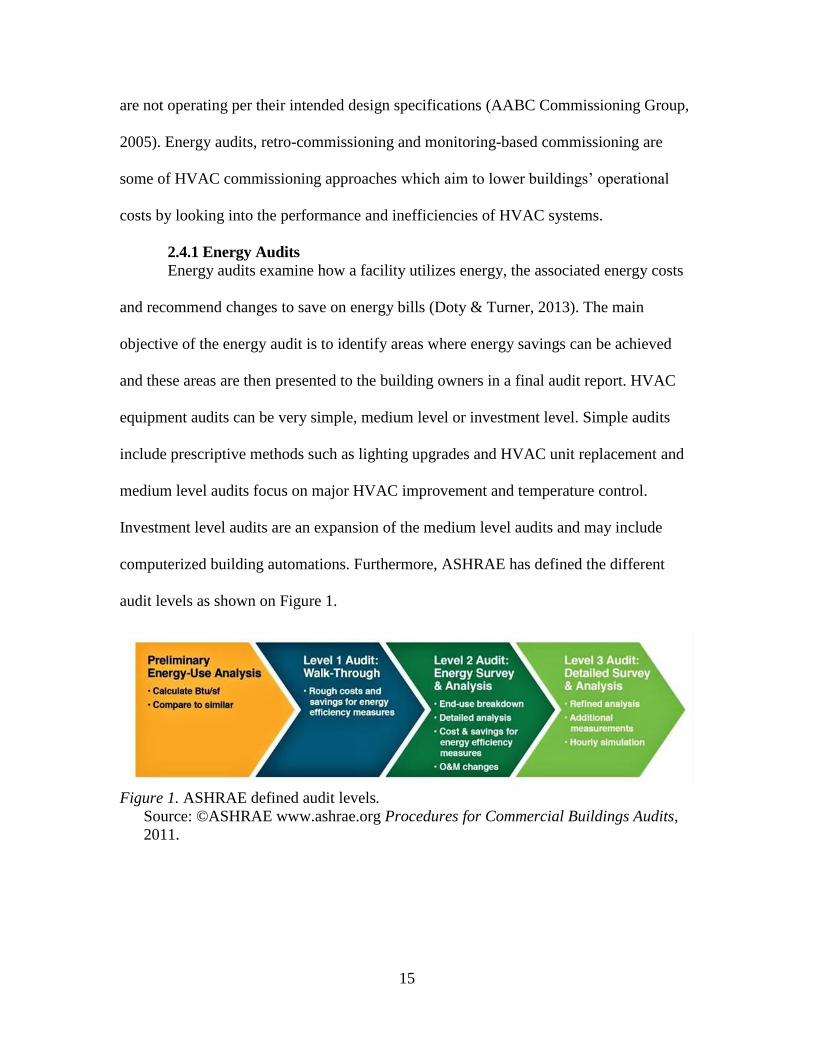
computerized building automations. Furthermore, ASHRAE has defined the different
audit levels as shown on Figure 1.
Figure 1. ASHRAE defined audit levels.
Source: ©ASHRAE www.ashrae.org Procedures for Commercial Buildings Audits,
2011.
16
Conducting an energy audit usually requires a 10-step process from the time the
initial facilities information is obtained to the moment the final audit report is created.
These 10 steps are listed below:
1. Obtain general facility information
2. Collect and evaluate utility bills
3. Develop a plan
4. Conduct a site survey
5. Develop a base model
6. Identify low cost options for energy savings
7. Identify energy conservation measures
8. Find interoperability opportunities among measures
9. Identify utility company/governmental incentives
10. Produce final audit report.
For collecting data, the energy auditor should collect energy consumption data for at
least a year preceding to the time the audit is being conducted (Doty & Turner, 2013)
including data on peripheral factors affecting energy use such as geographical location,
weather data and operating hours (Doty & Turner, 2013). During the site survey the
building operator is interviewed by the energy auditor to obtain building operations
information (e.g. when is the building occupied? are Air Handling Units shut down at
night?). Additionally, the onsite survey step includes acquiring specific Air Handling
Unit data such as supply air and outside air cubic feet per minute (CFM). Developing a
base model may include creating a bin analysis and computerized building simulation.
Bin Analyses model building energy consumption using HVAC equipment
17
characteristics. Computerized building automation programs model building performance
using analytical methods. All audits end with an audit report which is the culmination of
a 10- step process focusing on low cost energy savings approaches first and then growing
the energy saving solution to provide interoperability among many measures. The final
audit report should include an executive summary intended for non-technical upper
management officials. The building owners may or may not implement the
recommendations put forth in the audit report. It is important to note that the audit report
itself does not mean that implementation has taken place.
2.4.2 Retro-Commissioning Process
Retro-commissioning (RCx) is performed only to existing buildings that have
never gone through commissioning and focuses on equipment that uses energy to help
improve the energy efficiency. It is important to retro-commission a building because
unless professionally commissioned, virtually every building suffers from incomplete
setup during the construction process, especially the ones with highly technical controls
and operating systems (Thumann, Niehus, Younger, 2013). Although the objective of
retro-commission is to return the building to its intended design, this may be impossible
at times because original design documents may not be available (Doty & Turner, 2013).
Therefore, the intent of this praxis is to retro-commission existing HVAC equipment
using Guideline 36 as the new design framework to improve HVAC energy efficiency.
HVAC retro-commissioning can save energy through improving the functionality of
HVAC systems as well as fixing the problems that may have developed over the years.
Retro-commissioning is different from an energy audit because the energy saving
measures that are found by the commissioning team are implemented at once.
18
Since retro-commissioning is usually the next step after conducting an energy
audit, when a commissioning agent is called to perform retro-commissioning, one of their
objectives is to discover why energy parameters provided by the energy audit, such as the
Energy Use Index (EUI=Btu/sf-year) or the Energy Cost Index (ECI=Cost/sf-year),
within a specific facility may be higher than they should be (Thumann, Niehus, Younger,
2013). In a retro-commissioning process, many components are examined to determine
the biggest factors impacting energy usage. One of the most important components is the
current building occupancy and how functional the building spaces currently are rather
than focusing on what the original design intent was when the building was built. Space
usage can change over time and sometimes it changes frequently depending on the
building. Thus, commissioning agents cannot depend only on the building blueprints to
figure out how to fix the problems. It falls upon the commissioning agent to understand
how the space is currently being used so that they can reconfigure the system in order for
it to operate more efficiently. When conducting the retro-commissioning process, there
are four phases that the commissioning agent will follow. They are: (1) planning and
initial screening, (2) site assessment and investigation, (3) implementation of
recommended measures and (4) measurement and verification of result and final
reporting.
In the planning and initial screening phase, the commissioning agent determines if
the building is a good fit to go through the retro-commissioning process and makes sure
that it will bring substantial energy savings. To further determine if they should proceed
with retro-commissioning, commissioning agents gather utility bills, preliminary survey
information and discuss operations with facility personnel (Robinson, 2014) to get a
19
better understanding of the facility needs and come up with a preliminary retro-
commissioning plan. The preliminary RCx plan would include the projected energy
savings. RCx cost may also be generated as part of this phase (Robinson, 2014) so that
the building owners may make an educated business decision.
During the site assessment, the commissioning agent inspects the operation of the
current HVAC equipment and determines if there are operating deficiencies or
opportunities for energy conservation with a focus on low-cost measures (Robinson,
2014). The agent would also do simple repairs if needed. During the investigation phase,
the commissioning agent performs functional testing of HVAC equipment, evaluates the
performance as it relates to original design, and evaluates the condition of the current
control systems (Robinson, 2014). The agent may also analyze data from the Building
Automation System (BAS) to examine how the HVAC system is operating at its current
state.
During the phase of implementation of recommended measures most measures
will be implemented by the commissioning agent. There are cases where it may be
necessary to bring in an outside contractor where there are scope items that are not within
the expertise of the commissioning agent.
The last phase, measurement and verification of result and final reporting, is when
the commissioning agent checks to see how the equipment is performing with the
improvements that were made. There are measurements taken to evaluate the
performance such as the electric current strength, voltage, and power readings. The
commissioning agent will then document all the changes that were made through an
20
M&V [measurement and verification] report that documents the implementation of the
measures and the verified savings (Robinson, 2014).
2.4.3 Monitoring-Based Commissioning Process
Another existing building commissioning process is monitoring-based
commissioning (MBCx) and it is an ongoing process that keeps monitoring the energy
use of a building overtime with the same kind of practices that are used in retro-
commissioning. Monitoring-based commissioning involves the implementation of
improvements measures along with ongoing service and insights necessary for full
transparency, measurement, and reporting (Capehart & Brambley, 2015). The process
uses the Facility Management System (FMS) and allows the commissioning agent to
identify problems with building performance, and can suggest improvements that will
reduce building energy consumption and, in many cases, improve building comfort
(Capehart et al., 2015). It is also important to keep this commissioning process ongoing
to ensure the improved building comfort can be maintained. In doing so, ongoing
monitoring-based commissioning ensures that the initial results persist through seasonal
changes, different modes of operation, varying loads and other factors which can
contribute to decreased performance or improper operation (Capehart et al., 2015). This
study provides a prediction model that gives insights as to whether an Air Handling Unit
economizer sequence of operation is properly performing. Such prediction model that
may be used in an ongoing monitoring-based commissioning strategy since the model
may be used repeatedly by building owners. The ability to apply the model in different
seasons of the year allows the continuous monitoring of AHU efficiency over time.
21
2.5 ASHRAE Guideline 36
The intent of Guideline 36, entitled High Performance Sequences of Operation for
HVAC Systems, “is to provide uniform sequences of operation for heating, ventilating,
and air-conditioning (HVAC) systems that are intended to maximize HVAC system
energy efficiency and performance” (ASHRAE Guideline 36, 2018, Pg. 2).
Before ASHRAE Guideline 36, HVAC design engineers did not have a central
location for the specifications of HVAC systems sequences of operation. It was therefore
up to each engineer to custom-design their HVAC operations. While HVAC hardware
specifications has always been readily available, the HVAC controls were not specified
as a system, prior to ASHRAE G36.
All commissioning processes described thus far attempt to fine-tune the building as
designed by Engineer of Record. But ASHRAE Guideline 36 seeks to improve energy
efficiency by standardizing the initial design. By doing so, ASHRAE G36 also seeks to
lower the current dependency on proper systems implementation (construction process)
and commissioning process. Nevertheless, commissioning may remain a valuable, quality
management process because it can verify the initial implementation and ensure the
continuous adherence to the guideline. Guideline 36 can be broken down in three main
areas and they are: information, alarms and operations.
2.5.1 Information
The information category includes design information, information provided by
the engineer and information provided by the Testing and Balancing contractor. Fitting
this information together properly is the key to making the G36 sequences work as
intended.
22
2.5.1.1 Design Information
ASHRAE G36 states that HVAC engineers may obtain a Sequence of
Operations (SOO) for air handling units with multiple VAV systems only. Although
some air handling units may be equipped with enthalpy wheels, ASHRAE G36 does not
include design information for enthalpy wheels and there are no sequences of operations
templates written for them in the guideline. Enthalpy wheels are energy-saving devices
installed between the supply and return airstream of an air handling unit to recover heat
from the system. Enthalpy wheels are found more often in western Europe, and the
potential for using them in the United States is a topic for future research explored in
more detail in Chapter 6. Nevertheless, the fact that ASHRAE G36 does not include SOO
for enthalpy wheels does not impede the overall adoption of the guideline as engineers
may add their own sequences for enthalpy wheels.
2.5.1.2 Information Provided by the Engineer
The information provided by the engineer refers to the SOO specifications
that ASHRAE G36 indicates are to be included into the design documents. These
specifications include zone temperature setpoints, ventilation setpoints, zone groups, and
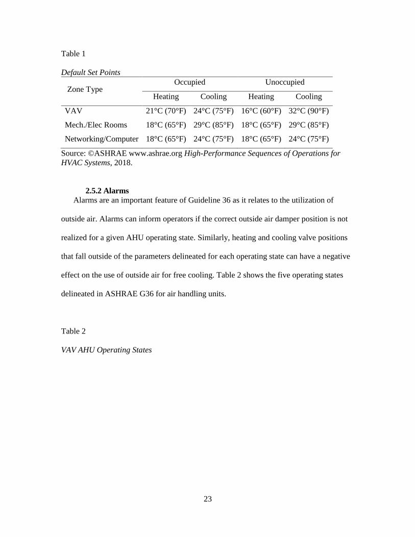
the economizer’s high limit. Table 1 shows the default set points included in ASHRAE
Guideline 36. For ventilation setpoints, G36 draws from the ASHRAE 62.1 Standard for
Ventilation Rate Procedures. These include a population component and an area
component in a room-by room and zone-by zone basis. Design engineers must calculate
how much fresh air is needed in each particular zone. Although it is designer’s
responsibility to determine CO₂ setpoints (ASHRAE Guideline 36, 2018) maximum
recommended CO₂ setpoints are also included, especially for cases where there is demand
controlled ventilation (DCV).
23
Table 1
Default Set Points
Zone Type Occupied Unoccupied
Heating Cooling Heating Cooling
VAV 21°C (70°F) 24°C (75°F) 16°C (60°F) 32°C (90°F)
Mech./Elec Rooms 18°C (65°F) 29°C (85°F) 18°C (65°F) 29°C (85°F)
Networking/Computer 18°C (65°F) 24°C (75°F) 18°C (65°F) 24°C (75°F)
Source: ©ASHRAE www.ashrae.org High-Performance Sequences of Operations for
HVAC Systems, 2018.
2.5.2 Alarms
Alarms are an important feature of Guideline 36 as it relates to the utilization of
outside air. Alarms can inform operators if the correct outside air damper position is not
realized for a given AHU operating state. Similarly, heating and cooling valve positions
that fall outside of the parameters delineated for each operating state can have a negative
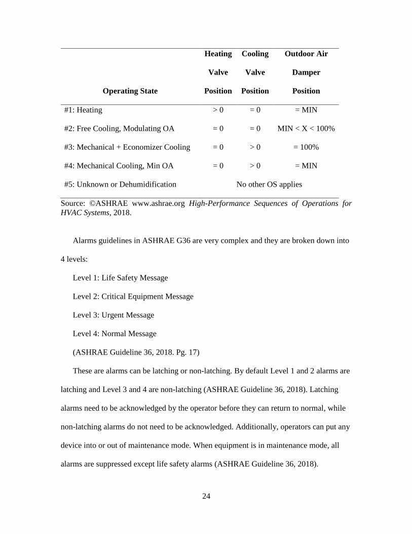
effect on the use of outside air for free cooling. Table 2 shows the five operating states
delineated in ASHRAE G36 for air handling units.
Table 2
VAV AHU Operating States
24
Operating State
Heating
Valve
Position
Cooling
Valve
Position
Outdoor Air
Damper
Position
#1: Heating > 0 = 0 = MIN
#2: Free Cooling, Modulating OA = 0 = 0 MIN < X < 100%
#3: Mechanical + Economizer Cooling = 0 > 0 = 100%
#4: Mechanical Cooling, Min OA = 0 > 0 = MIN
#5: Unknown or Dehumidification No other OS applies
Source: ©ASHRAE www.ashrae.org High-Performance Sequences of Operations for
HVAC Systems, 2018.
Alarms guidelines in ASHRAE G36 are very complex and they are broken down into
4 levels:
Level 1: Life Safety Message
Level 2: Critical Equipment Message
Level 3: Urgent Message
Level 4: Normal Message
(ASHRAE Guideline 36, 2018. Pg. 17)
These are alarms can be latching or non-latching. By default Level 1 and 2 alarms are
latching and Level 3 and 4 are non-latching (ASHRAE Guideline 36, 2018). Latching
alarms need to be acknowledged by the operator before they can return to normal, while
non-latching alarms do not need to be acknowledged. Additionally, operators can put any
device into or out of maintenance mode. When equipment is in maintenance mode, all
alarms are suppressed except life safety alarms (ASHRAE Guideline 36, 2018).
25
Entry Delays, Time Based Suppressions, Post Exit Suppressions and Exit Hysteresis
are also specified in ASHRAE Guideline 36. Entry delays denote the amount of time the
condition must exist before the alarm is triggered. Time based suppression, on the other
hand, tries to eliminate nuisance alarms that occur due to setpoint changes that have not
operated quickly. Similarly, after the alarm has triggered once, post exit suppression
limits alarms from triggering again for a certain amount of time depending on the alarm
level. Level 1 alarms have a 0 minute default suppression period and Level 4 alarms have
a 7 day period. Exit hysteresis delays the time to clear a triggered alarm until it remains
below the exit hysteresis setpoint for a determined amount of time.
Hierarchical alarm suppression was first described by Schein and Bushby in 2006,
and it is also included in Guideline 36. The idea is to create a hierarchical order for each
piece of equipment and their relationships with each other (i.e. “sources”, “loads” or
“systems”) (ASHRAE Guideline 36, 2018). For example, in a zone that is being supplied
by a VAV which is in turn is supplied by an Air Handler Unit, if the AHU breaks down,
the VAV zones will not trigger an alarm because the system recognizes that the fault is at
a higher level than the VAVs. Guideline 36 defines what these systems, sources, and
loads are. For example, a cooling tower is a system which is a source to the chiller. The
chillers are a system and source to the chilled water pumps. Chilled water pumps are a
system but also a load to the chillers and source to the air handlers.
The hierarchical alarm system is mainly run by a SystemOK flag. A SystemOK is
true when it is on, is achieving setpoint for five minutes and the system is ready to serve
its load (ASHRAE Guideline 36, 2018). A SystemOK is false when it is starting up and
not enough system component are available. By default, Level 1 through Level 3
26
component alarms will inhibit SystemOK but the operator shall have the ability to
determine SystemOK for different components (ASHRAE Guideline 36, 2018).
Automated Fault Detection Diagnostics (AFDD) is also a part of the alarm system
created in ASHRAE G36. For example, the description for Fault Condition (FC) #1 is
duct static pressure is too low with fan at full speed. This fault condition would trigger
and provide an alarm when the unit is in any state (OS#1-5). The guideline also provides
possible issues causing the alarm and in the case of FC#1 it could be a problem with the
Variable Frequency Drive (VFD) or the Supply Air Temperature Setpoint is too high.
Although this is a very complex alarm system that ASHRAE has put forth in Guideline
36, the intent is that in the future the AFDD provided herein become minimum standards
for HVAC design engineers to follow.
2.5.3 Operations
Guideline 36 specifies several different operational modes, and each contains
different settings that may affect the use of outside air for free cooling. In total, there are
seven control modes for the operation of Air Handling Units: (1) Occupied Mode, (2)
Cool-Down Mode, (3) Setup Mode, (4) Warmup Mode, (5) Setback Mode, (6) Freeze
Protection Setback Mode and (7) Unoccupied Mode. Each of these operation modes
contain several guidelines to follow regarding trim & respond static pressure, economizer
types, and freeze protection setback mode. Regardless of which operational mode the unit
is in, the most important guideline to follow is to sequence all control loops by a single
signal.
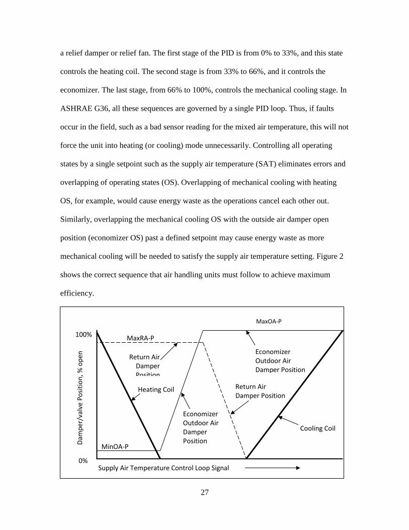
ASHRAE G36 recommends that the sequencing of mixed air, heating, and cooling
control be governed by the same signal, the supply air temperature (also known as
discharge air temperature). Figure 2 shows the supply air temperature loop mapping with
27
a relief damper or relief fan. The first stage of the PID is from 0% to 33%, and this state
controls the heating coil. The second stage is from 33% to 66%, and it controls the
economizer. The last stage, from 66% to 100%, controls the mechanical cooling stage. In
ASHRAE G36, all these sequences are governed by a single PID loop. Thus, if faults
occur in the field, such as a bad sensor reading for the mixed air temperature, this will not
force the unit into heating (or cooling) mode unnecessarily. Controlling all operating
states by a single setpoint such as the supply air temperature (SAT) eliminates errors and
overlapping of operating states (OS). Overlapping of mechanical cooling with heating
OS, for example, would cause energy waste as the operations cancel each other out.
Similarly, overlapping the mechanical cooling OS with the outside air damper open
position (economizer OS) past a defined setpoint may cause energy waste as more
mechanical cooling will be needed to satisfy the supply air temperature setting. Figure 2
shows the correct sequence that air handling units must follow to achieve maximum
efficiency.
Return Air Damper Position
Heating Coil
Economizer Outdoor Air Damper Position
MinOA-P
MaxRA-P
MaxOA-P
Economizer Outdoor Air Damper Position
Cooling Coil
Return Air Damper Position
100%
0%
Dam
per
/val
ve P
osi
tio
n, %
op
en
Supply Air Temperature Control Loop Signal
28
Figure 2. Supply air temperature loop mapping with relief damper or relief fan.
Source: ©ASHRAE www.ashrae.org High-Performance Sequences of Operations for
HVAC Systems, 2018
ASHRAE G36 proposes five different options for economizer high limits (1) Fixed Dry
Bulb, (2) Differential Dry Bulb, (3) Fixed Dry Bulb + Differential Dry Bulb, (4) Fixed
Enthalpy + Fixed Dry Bulb, (5) Differential Enthalpy + Fixed Dry Bulb (ASHRAE
Guideline 36, 2018). These different economizer options resulted in part due to a study
published in 2010 in the ASHRAE Journal called “Economizer High Limit Controls and
Why Enthalpy Economizers Don’t Work”. In that article the authors proposed that if
differential enthalpy alone is used, then when it got very humid outside moisture was being
introduced into the building. Differential enthalpy method measures both the outside air
enthalpy and the air handler’s return air enthalpy and uses the lower measurement as a
determining factor for which air supply (outside air or return air) to allow to enter the space
for conditioning purposes. Therefore, the authors proposed to add a high limit on the
Outside Air Temperature to disable the economizer when using it would increase the
Cooling Coil energy usage (Taylor, S. T., & Cheng, C. H., 2010). The study concluded
that depending where each system is located each economizer type has its various limitations
but for the most part the fixed enthalpy or differential enthalpy plus a dry-bulb limits were
almost always the best option.
Freeze Protection Setback Mode has multiple stages in ASHRAE G36. Stage 1
modulates the heating coil to maintain a minimum supply air temperature of 42˚ F
regardless whether the unit is in occupied mode or unoccupied mode. Stage 2 closes the
outdoor air damper for five minutes when sat drops below 38˚ f and the economizer and
outside air damper are closed for an hour with a Level 3 alarm notifying that minimum
29
outside air has been interrupted. Stage 3 shuts the fans down, opens the cooling coil valve
and start the chilled water pumps when SAT drops below 34˚ F for five minutes with a
Level 2 alarm notifying that the unit is shut down by freeze protection. (ASHRAE
Guideline 36, 2018).
There are many instances where Guideline 36 differs from the way most engineers
write sequences of operations for multizone AHUs. It does not necessarily mean, however,
that these SOO must all be implemented at once to make HVAC systems more efficient.
Rather, the first step is to understand the logic behind these guidelines before the changes
are implemented. ASHRAE G36 is to remain a guideline, not a standard, for the
foreseeable future because there are many buildings with older equipment that cannot
implement these sequences yet. Nevertheless, these guidelines will push the automation
and controls companies to deliver better products and eventually some aspects of Guideline
36 may be adopted into an existing ASHRAE standard.
30
Chapter 3 - Methods
3.1 Overview
This is a quantitative research study. Quantitative research is ideal for studying the
relationships between variables and phenomena that can be isolated and quantified
(Borrego, Douglas, & Amelink, 2009). In this study, the data consist of air handling system
trend logs that are recorded in quantitative form. This makes a quantitative approach ideal
for dealing with the data. Individual parameters are naturally measured in quantitative
form, and numerous quantitative measures of energy efficiency for HVAC systems already
exist (Du et al., 2016). In addition, energy efficiency itself is an issue of the relationship
between variables—namely, the relationship between a system’s energy input and its
heating, cooling, and/or ventilation output.
While subjective, qualitative data could be useful for exploring the effects of improving
the energy efficiency on the comfort of building occupants, this topic is beyond the scope
of the present study, which is instead primarily concerned with energy efficiency itself. A
qualitative approach would therefore be a poor fit.
The three specific statistical analyses will be non-experimental using historical data.
Ideally, quantitative research should be experimental to draw causal conclusions about the
relationships that may be identified (Johnson, 2001). However, this is often not feasible
because the study variables cannot be ethically and/or feasibly manipulated by the
researcher. In this case, experimental manipulation of large-scale HVAC use in commercial
buildings is significantly beyond the researcher’s practical ability to manipulate. However,
correlational data still provides useful information about the relationships between
variables (Johnson, 2001). While correlations do not necessarily imply causation, the
31
existence of a correlational relationship between variables still implies that one has
predictive power over another, creating a model with real-world relevance. In the case of
this study, a correlational relationship should be enough to determine whether or not the
system is functioning according to ASHRAE Guideline 36, as it suggests that certain levels
of input should create certain levels of output (ASHRAE, 2017). Thus, if the inputs and
outputs are not correlated as expected, then it can be determined that there is a breakdown
in the application of the guideline to the system.
In this case, the historical approach is the most appropriate as HVAC systems records
should create a significant sample size from purely historical data, limiting the need to
collect data and allowing for efficient analysis (Johnson, 2001). This makes historical
studies ideal when such a collection of data is existent and accessible to the researcher.
Therefore, this study was conducted with data collected by building owners and the
data was analyzed to examine energy savings of an AHU after being commissioned per
Guideline 36. The study utilizes three types of statistical analyses to thoroughly examine
the effectiveness of the guideline. The three statistical analyses were developed to answer
the following research questions:
1. Is there a greater use of Outside Air (free cooling) after adoption of ASHRAE
Guideline 36?
2. Is there a difference in energy use for building cooling before and after adoption of
ASHRAE Guideline 36?
3. Can a model be developed to let building owners know the AHU system is working
in compliance with ASHRAE Guideline 36 as it relates to economizer sequences of
operations/free cooling?
32
The following hypotheses were formulated to answers the research questions:
H1: Adoption of ASHRAE Guideline 36 leads to higher utilization of Outside Air.
H2: Adoption of ASHRAE Guideline 36 leads to higher energy efficiency.
H3: A prediction model will provide insights as to whether an AHU economizer
sequence of operation is properly performing.
3.2 Data Collection, Processing, and Analysis
The data for this study was extracted from a Building Management Systems (BMS)
currently servicing the building where the AHU is located. The BMS records trend logs for
various hardware devices and software parameters on a time schedule that varies from 15
minutes to hourly. The data was then uploaded into a data warehouse where it is available
for further processing. Appendix A contains a representative sample of the dataset used in
this study. The data set includes:
1. Outside Air Damper Actuator Position (MAXOAD). The degree to which the
HVAC system’s outside airflow is dampened at a given Outside Air Temperature.
2. Heating Coil Actuator Position (AHA2HCVPOS). The degree to which the HVAC
Heating Coil valve opens and closes at a given Outside Air Temperature.
3. Cooling Coil Actuator Position (AHA2CCV1POS). The degree to which the
HVAC Cooling Coil 1 valve opens and closes at a given Outside Air Temperature.
4. Cooling Coil Actuator Position (AHA2CCV2POS). The degree to which the
HVAC Cooling Coil 2 valve opens and closes at a given Outside Air Temperature.
5. Cubic Feet per Minute (AHA2CFM). The number of cubic feet of air that the
HVAC system processes per minute.
6. Mixed Air Temperature (AHA2MAT). The temperature of the air as the returned
air mixes with the supply air.
33
7. Supply Air Temperature (AHA2SAT). The temperature of the air that is supplied at
the space.
8. Preheat Coil Temperature (AHA2PHCT). The temperature to which the HVAC
system’s preheat coil is heated.
9. Outside Air Humidity (OAH). The humidity level of the Outside Air.
10. Outside Air Temperature (OAT). The temperature as measured outside the
building.
Because these data are real physical quantities they can only be measured in terms of a
unit for the appropriate quantity—for example, temperature could be measured in
Fahrenheit, Celsius, Kelvin, or Rankin, but all these scales are units of temperature.
Therefore, appropriate conversion must be used to ensure that all final data are recorded in
consistent units prior to analysis.
In this study, the AHU operational data was gathered from September of 2016 to March
of 2017 prior to the adoption of the Guideline 36 to ensure all seasons were collected.
Similarly, the AHU operational data was collected from September of 2017 to March of
2018 after the adoption of the Guideline 36. Then, several steps were taken to properly
screen the data that most reflected the HVAC unit actual operational conditions during
occupied times. This process was necessary because sequences of operations change
between occupied and unoccupied times.
The selection criteria to obtain operational data during occupied times were:
1. Filter and keep in the dataset the data for weekdays only (Monday through Friday).
2. Filter and keep in the dataset the data to 9am to 5pm only.
3. Filter and keep in the dataset the data when free outside cooling was available.
34
4. Filter and remove from the dataset the data collected during the time the unit was
known to be in downtime period for maintenance related work.
5. Filter and remove from the dataset periods of false recordings due to sensor
malfunctioning (e.g. if damper position falls below 3, which means it is less than
30% open, that observation would be removed because per building code the
minimum fresh air intake should be 30% coming into the space being conditioned)
Once the data was filtered, it was entered IBM SPSS software for analysis purposes.
Lastly, this study ensured that the data was complete and with the correct units of
measurement and significant figures being the same across the entire dataset. Once the
filtering process had been carried out, data analysis was conducted.
3.3 Statistical Analysis # 1
The first statistical analysis used in this study includes both a linear and a non-linear
(quadratic) regression analysis to provide evidence that greater modulation of the outside
air damper (OAD) in relationship to the outside air temperature (OAT) occurs under
ASHRAE G36, thus achieving more free cooling from the outside air (OA). To visually
detect which regression model is the best fit for the dataset, a plot containing OAD as
dependent variable (Y- axis) and OAT as independent variable (X-axis) was generated. The
accepted overall significance for the regression models is less than .05 (p-value <.05). The
normality of residuals assumption was performed for the linear regression analyses
conducted before and after adoption of G36.
The OAD variable was the dependent variable, and it was measured on a scale from 1
through 10, with 10 indicating that the damper position is completely open and thus
allowing exterior air to enter the unit and 1 meaning the damper position is completely
closed preventing any Outside Air from entering the unit. Building codes require that a
35
minimum amount of Outside Air always enters the space being air-conditioned. The
minimum amount of OA varies depending on the type of space. The air handling unit used
for this study serves different types of rooms including trash rooms, office spaces, locker
rooms, and kitchens. Some spaces require average outside air intake (22% OA), while other
spaces require up to 56% OA. Consistently, the AHU adjusts the OA intake requirement
accordingly to bring in the required amount of OA (roughly 39% OA) to all spaces being
used. For this study the minimum amount OA used was 30% OA (damper position #3) as
a conservative minimum OA point because not all rooms are always occupied, and the
ventilation efficiency fluctuates accordingly. Generally, if a damper position fell below the
30% open position this was an indication of bad sensor reading or that the unit outside air
damper actuator was malfunctioning. Therefore, damper position values below 3 were not
used for this study. The OAT is the independent variable and it is measured in degrees
Fahrenheit. The main range of outside temperature used for free cooling is between 0°F-
65°F. Temperatures below this range may cause freeze condition to the HVAC unit and
will also require energy to heat up the air to meet comfortable temperatures. Temperatures
above this range may require mechanical cooling to cool down the Outside Air, the Return
Air or a mixture of the two to a desired temperature thus defeating the purpose of true
economizer energy savings.
3.4 Statistical Analysis # 2
The second statistical analysis used in this study compared the mechanical cooling
loads used by the air handling unit before and after the guideline adoption. Mechanical
cooling loads were determined based on the amount of heat gain (in BTUs) the unit must
offset. BTUs were converted into tonnage of mechanical cooling by simply dividing the
BTUs by 12,000 since 1 ton of mechanical cooling can cool up to 12,000 BTUs. The pre-
36
G36 period that was used to conduct this analysis was September-December 2016. The
post-G36 period was September-December 2017.
In economizer cycles, the switchover point may be accomplished by either sensing the
outdoor dry bulb (DB) temperature (Outdoor Temperature Method) or sensing outdoor and
return air enthalpy (Enthalpy Switchover Method) (United States Environmental Protection
Agency, 2001). The unit in this study used the outdoor temperature method for economizer
control with a temperature limit of 70° F. Appendix B contains the AHU controls
specifications, the control syntax, and the syntax explanation for the economizer sequence
used in this study.
The BTU calculations for the outdoor dry bulb temperature switchover method are
broken down into two steps:
1. When outdoor air temperature is less than 40˚f, the air entering the cooling coil will
have a temperature of 64.5˚f.
2. When the outdoor air temperature is between 40˚f and 56.5˚f degrees, the air
entering the cooling coil will have a temperature of 67˚F (United States
Environmental Protection Agency, 2001)
The following equation was used to obtain the BTUs for an HVAC system in heating
mode:
1. BTUs = CFM * 1.08 * Temperature Delta
Temperature delta refers to the difference between air entering the cooling coil (a
combination of mixed air temperature and outside air temperature) and the supply air
temperature setting. Typically, the designed static Supply Air Temperature Setpoint is 55˚F
for many HVAC units. However, in Guideline 36, ASHRAE proposes that the modulation
37
of that setpoint contributes to OA free cooling utilization. For this research we used
average temperatures entering the Cooling Coil when the outside air is below 40˚ F and
above 40˚F and these averages are 64.5˚F and 67˚F respectively (United States
Environmental Protection Agency, 2001).
However, the mechanical cooling data obtained did not have a normal distribution and
a two-step rank transformation was performed to achieved normalized mechanical cooling
data. Using a two-step rank transformation is appropriate for continuous variables such as
the mechanical cooling tons data (Templeton, 2011). Tests for normality and equality of
variances were conducted on the newly created normalized mechanical cooling tons
variable. A comparison of the means for normalized mechanical cooling loads before and
after adoption of guideline 36 was achieved by conducting an independent samples t-test.
To avoid a false attribution to the guideline (that is, to confirm the energy savings were
not due to a more favorable season), weather data was obtained from a nearby weather
station for the same timeframes that were used to perform the mechanical cooling
calculations before and after the guideline adoption. For both periods, the weather data
exhibited non-normal distributions, and thus a non-parametric test such as the Mann-
Whitney Test was most appropriate. To ensure the Mann-Whitney test results were valid, a
test for homogeneity was performed on the weather data set. If similar weather patterns (in
this case equal median temperatures), before and after Guideline 36 adoption are observed,
then the AHU mechanical cooling usage should be similar as well if no change was caused
by adoption of Guideline 36.
3.5 Statistical Analysis # 3
The third statistical analysis used in this study was a multiple linear regression analysis
culminating in a model that building owners can use to gain insights as to whether the
38
AHU economizer sequence of operations is performing properly. The multiple linear
regression analysis was performed by following four steps:
1. Formulating the problem
2. Fitting the model
3. Validating assumptions
4. Evaluating the fitted model
(Chatterjee, S., & Hadi, A. S., 2015)
3.5.1 Formulating the problem
The purpose of the study is to identify which factors predict the dependent variable, the
outside air damper (OAD) position, to determine if the air handling unit sequence of
operations aligns with the expectations of ASHRAE G36. For this study, the OAD variable
description is MAX.OAD. Each independent variable also has specific descriptions. The
Heating Coil variable description is AHA2HCPOS. The Cooling Coil 1 and Cooling Coil 2
variable description are AHACCV1POS and AHACCV2POS, respectively. For the Preheat
Coil Temperature the variable description is AHA2PHCT. For the Total Supply CFM, the
variable description is AHA2CFM. For the Mixed Air, the variable description is
AHA2MAT. For the Supply Air Temperature, the variable description is AHA2SAT. For
the Outside Air Temperature, the variable description is OAT. For the Outside Air
Humidity, the variable description is OAH.
3.5.2 Fitting the Model
To obtain the model that best fit the data, multiple iterations of the regression model
were conducted with different combinations of the independent variables. This multiple
iteration process allowed for a model that was the most statistically significant and the most
powerful in predicting the dependent variable. The acceptable p-value for each predictor
39
used in the multiple linear regression model is less than .05 (p-value < .05). The accepted
overall significance for the regression model is less than .05 (p-value <.05) as well.
Adjusting the equation for this study results in the following equation:
MAXOAD = a + m(AHA2HCVPOS) + n(AHA2CCV2POS) + o(AHA2CFM) +
p(AHA2CCV1POS) + q(AHA2MAT) + r(AHA2SAT) + s(AHA2PHCT) + t(OAH) +
u(OAT)
where:
MAXOAD = AHA2.MAXOAD (the dependent variable)
m, n, o, p, q, r, s, t, u, v, w = the slope of the line from the regression analysis
a = the Y intercept or constant
3.5.3 Validating Assumptions
Multiple linear regression has the following inherent assumptions that must be
thoroughly checked to ensure the reliability of the results obtained:
1. Sample Size
2. Multicollinearity
3. Outliers
4. Homoscedasticity
5. Normality
There are differing schools of thought for determining the correct sample size when
conducting linear regression. For example, it is commonly accepted that 30 observations or
subjects are the minimum accepted sample size. According to Tabachnick & Fidell (2007),
50 cases plus eight times the number of independent variables is necessary. However,
Pearson (2009) states that 400 observations or more are sufficient for detecting all but the
smallest effects. The sample size used for this exercise was 17,322 observations.
40
Multicollinearity refers to the relationship among independent variables (Pearson,
2009). No variable with a bivariate correlation higher than .70 was used in this study. In
addition, the tolerance values for all predictors will not be below .10 and Variance Inflation
Factors (VIFs) should not be above 10 (Pearson, 2009). However, predictors with VIFs
values greater than 5 may not be accepted in practical applications. This study will only test
the reliability and prediction ability of the multiple regression model with predictors that
have VIFs values below 5.
Outliers that appear outside the rest of the data were carefully examined, and those
outliers that represented bad sensor readings or equipment downtime were removed from
the dataset to enable the regression analysis. Homoscedasticity assumes that the variance of
the residuals of the dependent variable is similar across the predicted values of the
dependent variable. If heteroscedasticity occurs, it can be observed in the scatterplot for
standardized residuals plotted against the standardized predicted values. Multiple linear
regression assumes that the residuals of the regression are normally distributed. To check
for this assumption, a regression standardized residuals histogram was created and a normal
P-P plot of regression standardized residual was conducted.
To ensure the model’s prediction power, predicted values were compared against the
actual values obtained post-Guideline 36 adoption by conducting a paired sample t-test. A
paired samples t-test is significant when the p-value is less than 0.05. The paired samples t-
test produced a statistically significant result of 0.000. However, there are several
assumptions that must be met to ensure the validity of the paired samples t-test. For
example, the dependent variables must be continuous, and the differences should be
approximately normally distributed. However, when testing the differences between the
41
predicted values produced by the model and the actual values obtained from the AHU after
G36 adoption, the Shapiro-Wilk Test produced a statistically significant result of .000,
suggesting that the differences were not normally distributed. Therefore, a Wilcoxon-
Signed-Rank test was conducted between the predicted values of the model and the actual
values obtained by the AHU during operations after G36 implementation. The Wilcoxon-
Signed Rank test tested the null hypothesis that difference of the median predicted values
and the actual OAD values equals 0.
The multiple linear regression model was then applied to the dataset collected prior to
the adoption of ASHRAE Guideline 36 from the same AHU to establish the difference, if
any, between the predicted and the actual position of the outside air damper (OAD) during
occupied times. A Wilcoxon Signed-Rank test was also performed to compare the
predicted versus the actual values.
3.6 Study Delimitations and Ethical Considerations
The study is delimited to one Multizone Air Handling Unit system used in a
commercial building in a specific geographic region for a period of one year before and
after implementing ASHRAE Guideline 36. These exact results may not extend to other
AHUs located in other regions due to many factors affecting economizer efficiency in other
geographical locations. However, the analytical approach would still apply. The
commissioning of AHUs is a heavy resource-consuming process, and obtaining the
approval of building owners can be very difficult. The AHU data used in this study was
previously generated during the unit’s recommissioning.
The study does not involve human subjects, limiting the ethical considerations
necessary. Indeed, the results of the study will have the potential to benefit the building
owners by making them aware of possible inefficiencies in their HVAC systems. This
42
study will not provide the participating building owners’ name or place of business to
ensure that participation in this research does not reveal any potentially sensitive data to
competitors or do harm to the participating building owners. Overall, the study is expected
to be of minimal risk and may offer potential practical benefits.
43
Chapter 4 – Results
4.1 Overview
This chapter contains the results of all three statistical analyses performed in this
study. The first statistical analysis consists of the linear and non-linear regressions
examining the relationship between the outside air damper and the outside air
temperature. The second analysis is a comparison between the AHU’s mechanical
cooling utilization before and after the adoption of ASHRAE G36. The final statistical
analysis is the multiple linear regression used to create the prediction model for building
owners at the end of this chapter.
4.2 Results of Statistical Analysis #1
The first statistical analysis was undertaken to identify if adopting ASHRAE G36
contributes to a greater modulation of the outside air damper position (MAX.OAD) relative
to the outside air temperature (OAT), which would lead to greater utilization of the outside
air for free cooling. Figure 3 contains a visual representation of the non-statistically
significant linear relationship between OAT and MAX.OAD before G36 adoption. The
statistically significant quadratic relationship between MAX.OAD and OAT before G36 is
shown in Figure 3.
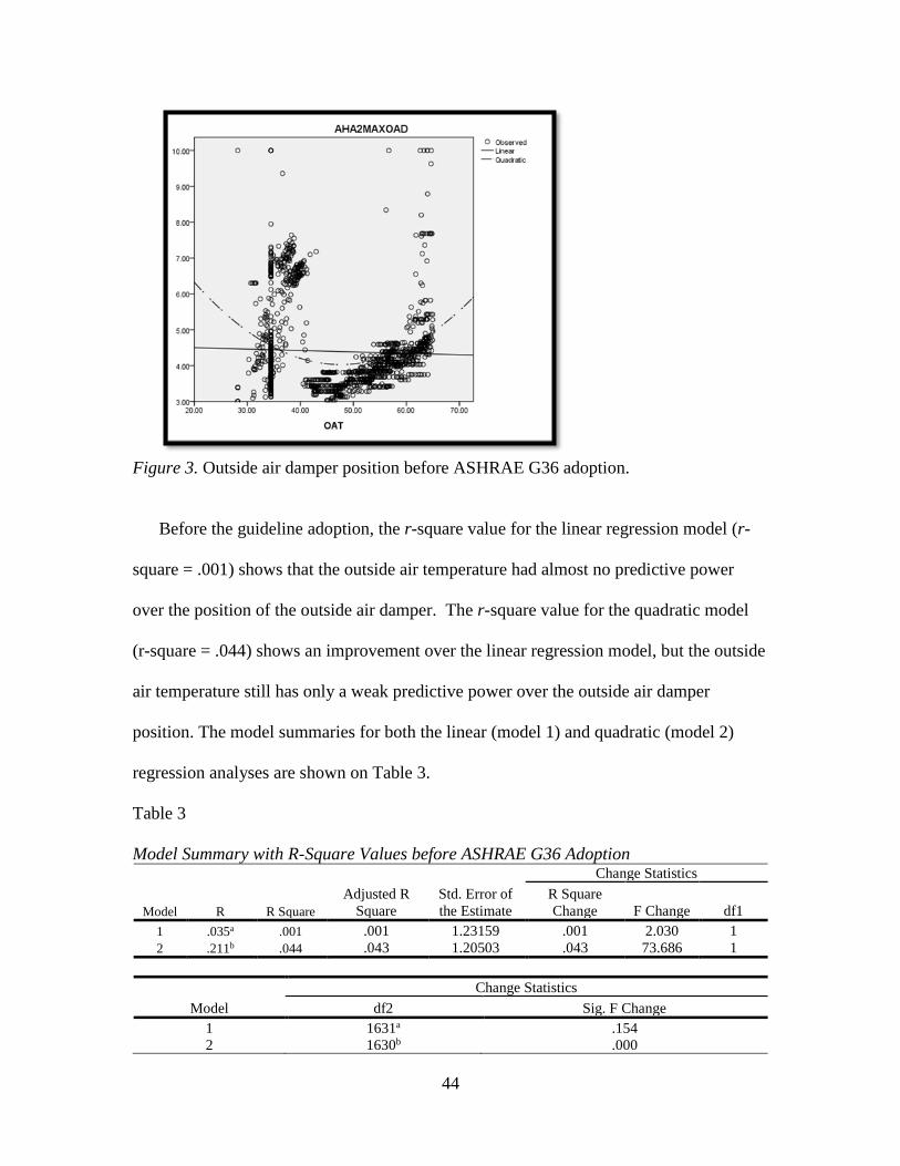
44
Figure 3. Outside air damper position before ASHRAE G36 adoption.
Before the guideline adoption, the r-square value for the linear regression model (r-
square = .001) shows that the outside air temperature had almost no predictive power
over the position of the outside air damper. The r-square value for the quadratic model
(r-square = .044) shows an improvement over the linear regression model, but the outside
air temperature still has only a weak predictive power over the outside air damper
position. The model summaries for both the linear (model 1) and quadratic (model 2)
regression analyses are shown on Table 3.
Table 3
Model Summary with R-Square Values before ASHRAE G36 Adoption
Model R R Square
Adjusted R
Square
Std. Error of
the Estimate
Change Statistics
R Square
Change F Change df1
1 .035a .001 .001 1.23159 .001 2.030 1
2 .211b .044 .043 1.20503 .043 73.686 1
Model
Change Statistics
df2 Sig. F Change
1 1631a .154
2 1630b .000
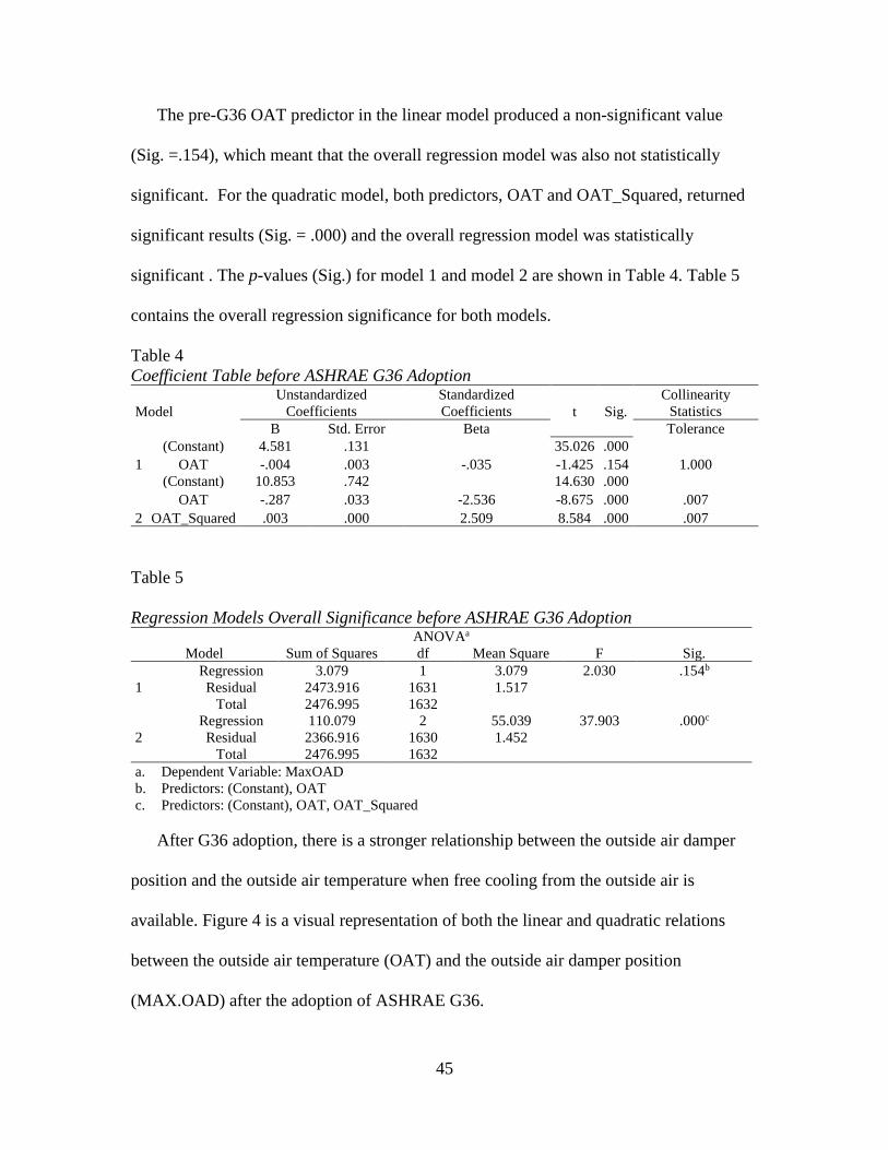
45
The pre-G36 OAT predictor in the linear model produced a non-significant value
(Sig. =.154), which meant that the overall regression model was also not statistically
significant. For the quadratic model, both predictors, OAT and OAT_Squared, returned
significant results (Sig. = .000) and the overall regression model was statistically
significant . The p-values (Sig.) for model 1 and model 2 are shown in Table 4. Table 5
contains the overall regression significance for both models.
Table 4
Coefficient Table before ASHRAE G36 Adoption
Model
Unstandardized
Coefficients
Standardized
Coefficients t Sig.
Collinearity
Statistics
B Std. Error Beta Tolerance
1
(Constant) 4.581 .131 35.026 .000
OAT -.004 .003 -.035 -1.425 .154 1.000
2
(Constant) 10.853 .742 14.630 .000
OAT -.287 .033 -2.536 -8.675 .000 .007
OAT_Squared .003 .000 2.509 8.584 .000 .007
Table 5
Regression Models Overall Significance before ASHRAE G36 Adoption ANOVAa
Model Sum of Squares df Mean Square F Sig.
1
Regression 3.079 1 3.079 2.030 .154b
Residual 2473.916 1631 1.517
Total 2476.995 1632
2
Regression 110.079 2 55.039 37.903 .000c
Residual 2366.916 1630 1.452
Total 2476.995 1632
a. Dependent Variable: MaxOAD
b. Predictors: (Constant), OAT
c. Predictors: (Constant), OAT, OAT_Squared
After G36 adoption, there is a stronger relationship between the outside air damper
position and the outside air temperature when free cooling from the outside air is
available. Figure 4 is a visual representation of both the linear and quadratic relations
between the outside air temperature (OAT) and the outside air damper position
(MAX.OAD) after the adoption of ASHRAE G36.
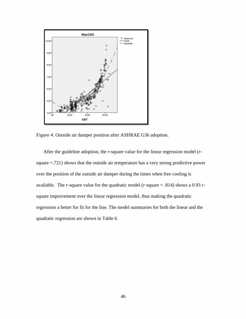
46
Figure 4. Outside air damper position after ASHRAE G36 adoption.
After the guideline adoption, the r-square value for the linear regression model (r-
square =.721) shows that the outside air temperature has a very strong predictive power
over the position of the outside air damper during the times when free cooling is
available. The r-square value for the quadratic model (r-square = .814) shows a 0.93 r-
square improvement over the linear regression model, thus making the quadratic
regression a better for fit for the line. The model summaries for both the linear and the
quadratic regression are shown in Table 6.
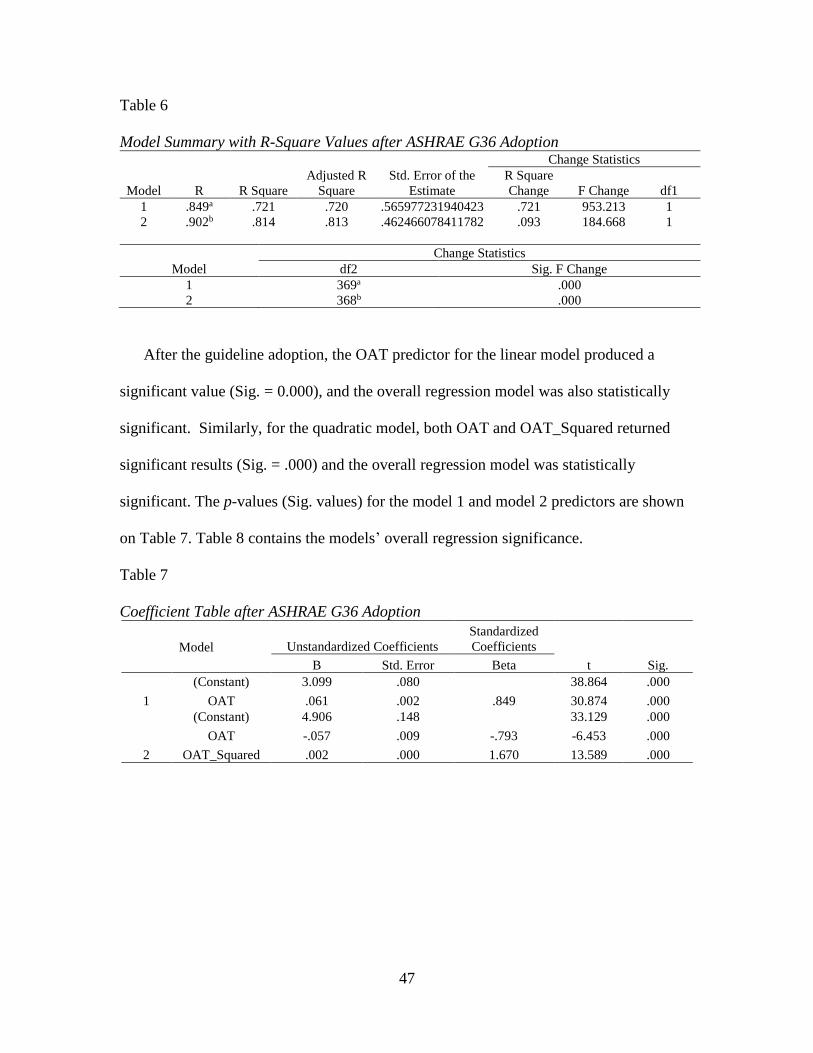
47
Table 6
Model Summary with R-Square Values after ASHRAE G36 Adoption
Model R R Square
Adjusted R
Square
Std. Error of the
Estimate
Change Statistics
R Square
Change F Change df1
1 .849a .721 .720 .565977231940423 .721 953.213 1
2 .902b .814 .813 .462466078411782 .093 184.668 1
Model
Change Statistics
df2 Sig. F Change
1 369a .000
2 368b .000
After the guideline adoption, the OAT predictor for the linear model produced a
significant value (Sig. = 0.000), and the overall regression model was also statistically
significant. Similarly, for the quadratic model, both OAT and OAT_Squared returned
significant results (Sig. = .000) and the overall regression model was statistically
significant. The p-values (Sig. values) for the model 1 and model 2 predictors are shown
on Table 7. Table 8 contains the models’ overall regression significance.
Table 7
Coefficient Table after ASHRAE G36 Adoption
Model Unstandardized Coefficients
Standardized
Coefficients
t Sig. B Std. Error Beta
1
(Constant) 3.099 .080 38.864 .000
OAT .061 .002 .849 30.874 .000
2
(Constant) 4.906 .148 33.129 .000
OAT -.057 .009 -.793 -6.453 .000
OAT_Squared .002 .000 1.670 13.589 .000
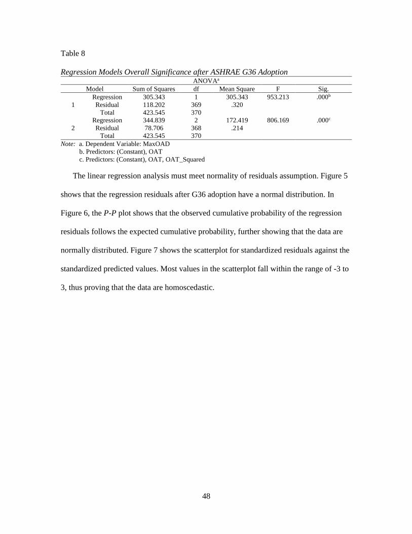
48
Table 8
Regression Models Overall Significance after ASHRAE G36 Adoption ANOVAa
Model Sum of Squares df Mean Square F Sig.
1
Regression 305.343 1 305.343 953.213 .000b
Residual 118.202 369 .320
Total 423.545 370
2
Regression 344.839 2 172.419 806.169 .000c
Residual 78.706 368 .214
Total 423.545 370
Note: a. Dependent Variable: MaxOAD
b. Predictors: (Constant), OAT
c. Predictors: (Constant), OAT, OAT_Squared
The linear regression analysis must meet normality of residuals assumption. Figure 5
shows that the regression residuals after G36 adoption have a normal distribution. In
Figure 6, the P-P plot shows that the observed cumulative probability of the regression
residuals follows the expected cumulative probability, further showing that the data are
normally distributed. Figure 7 shows the scatterplot for standardized residuals against the
standardized predicted values. Most values in the scatterplot fall within the range of -3 to
3, thus proving that the data are homoscedastic.
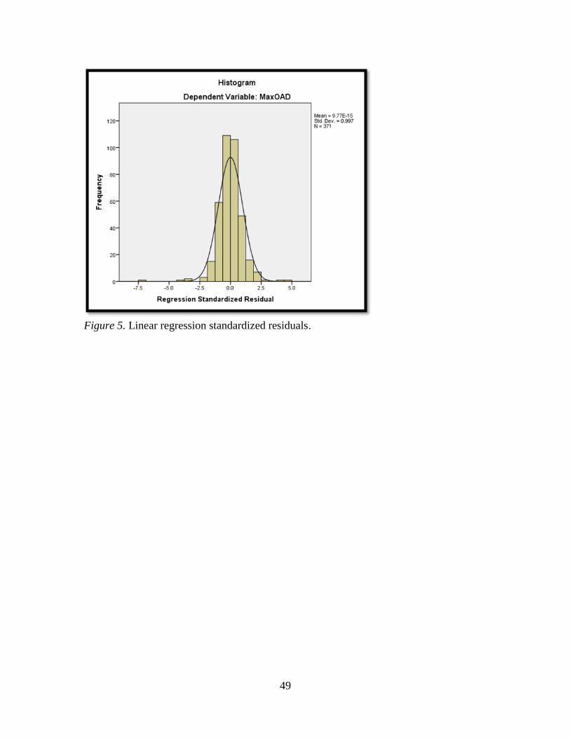
49
Figure 5. Linear regression standardized residuals.
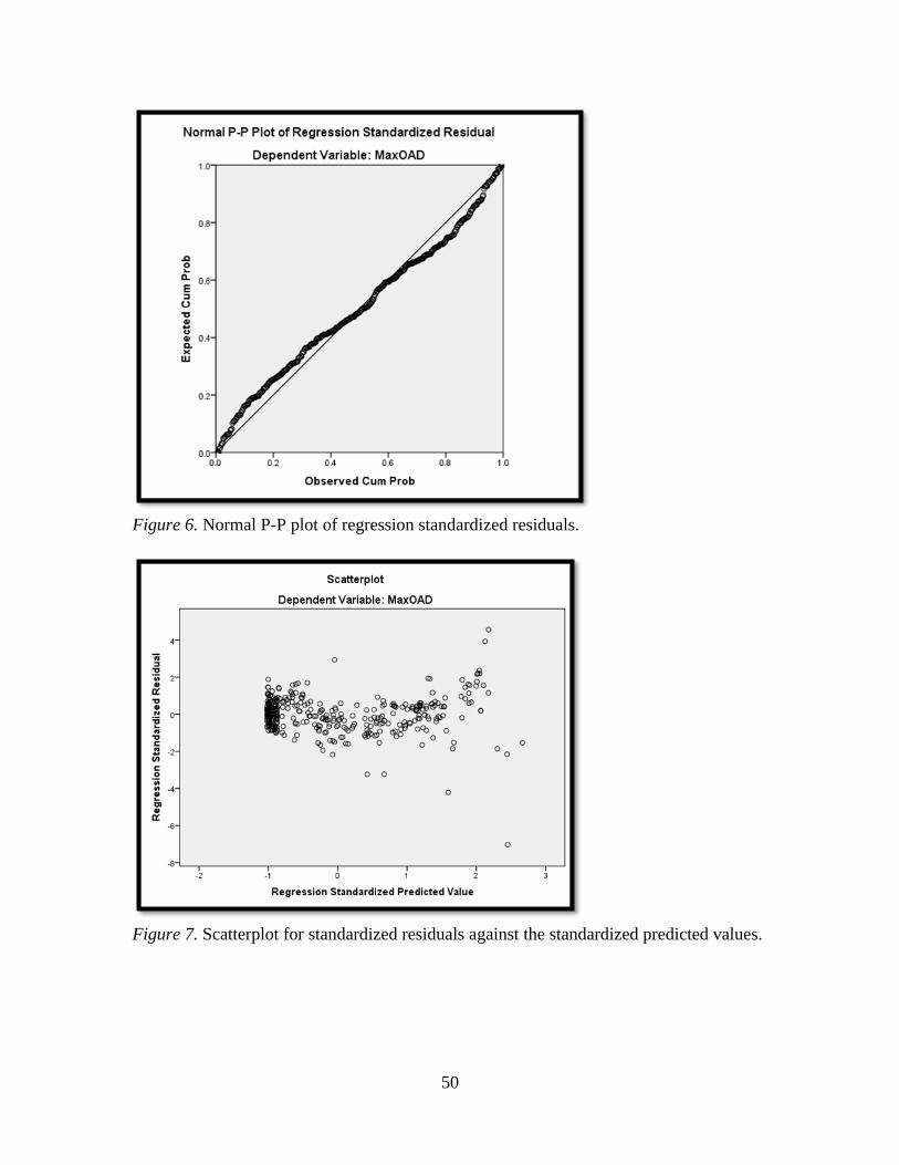
50
Figure 6. Normal P-P plot of regression standardized residuals.
Figure 7. Scatterplot for standardized residuals against the standardized predicted values.
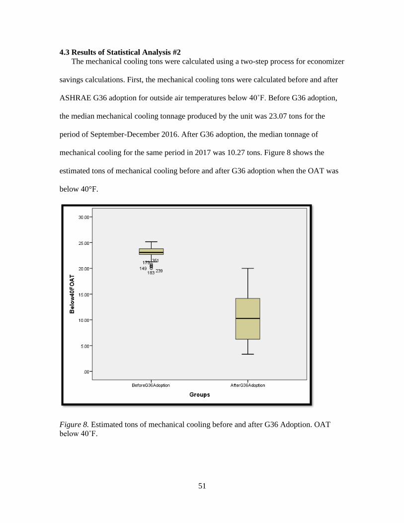
51
4.3 Results of Statistical Analysis #2
The mechanical cooling tons were calculated using a two-step process for economizer
savings calculations. First, the mechanical cooling tons were calculated before and after
ASHRAE G36 adoption for outside air temperatures below 40˚F. Before G36 adoption,
the median mechanical cooling tonnage produced by the unit was 23.07 tons for the
period of September-December 2016. After G36 adoption, the median tonnage of
mechanical cooling for the same period in 2017 was 10.27 tons. Figure 8 shows the
estimated tons of mechanical cooling before and after G36 adoption when the OAT was
below 40°F.
Figure 8. Estimated tons of mechanical cooling before and after G36 Adoption. OAT
below 40˚F.
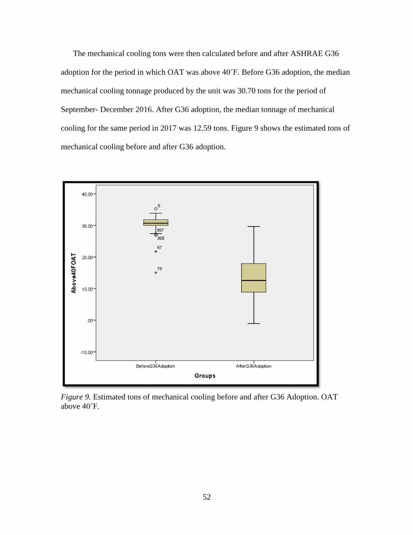
52
The mechanical cooling tons were then calculated before and after ASHRAE G36
adoption for the period in which OAT was above 40˚F. Before G36 adoption, the median
mechanical cooling tonnage produced by the unit was 30.70 tons for the period of
September- December 2016. After G36 adoption, the median tonnage of mechanical
cooling for the same period in 2017 was 12.59 tons. Figure 9 shows the estimated tons of
mechanical cooling before and after G36 adoption.
Figure 9. Estimated tons of mechanical cooling before and after G36 Adoption. OAT
above 40˚F.
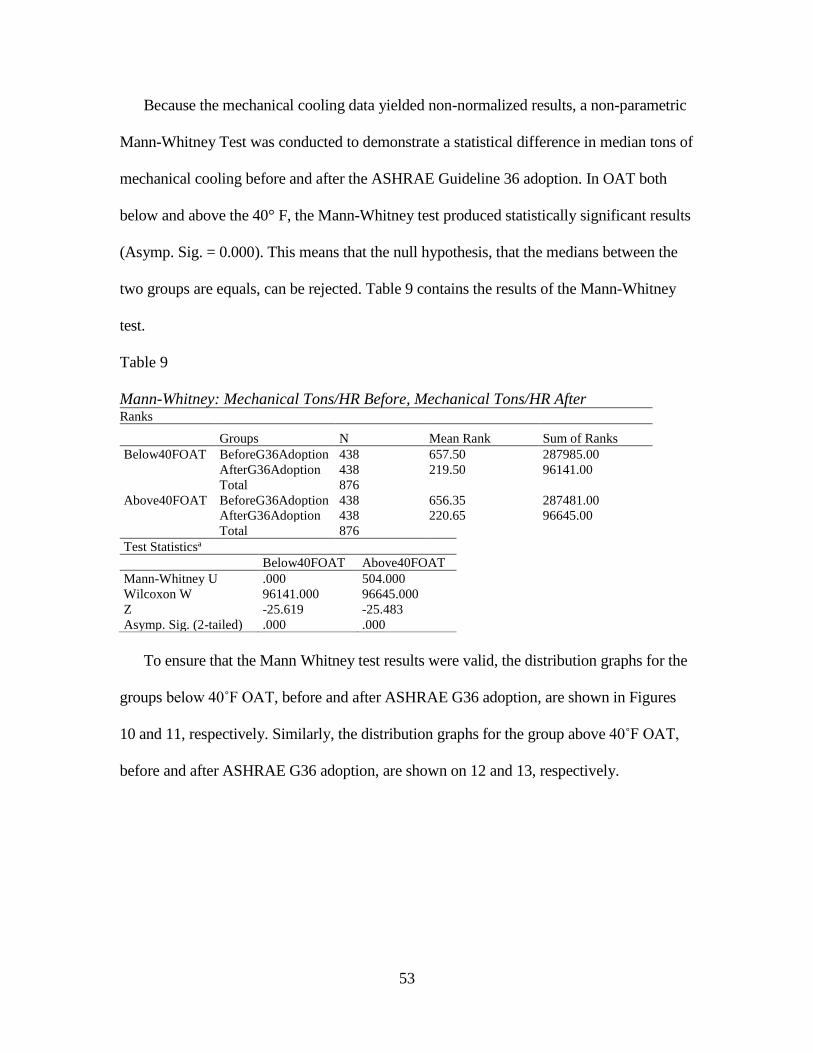
53
Because the mechanical cooling data yielded non-normalized results, a non-parametric
Mann-Whitney Test was conducted to demonstrate a statistical difference in median tons of
mechanical cooling before and after the ASHRAE Guideline 36 adoption. In OAT both
below and above the 40° F, the Mann-Whitney test produced statistically significant results
(Asymp. Sig. = 0.000). This means that the null hypothesis, that the medians between the
two groups are equals, can be rejected. Table 9 contains the results of the Mann-Whitney
test.
Table 9
Mann-Whitney: Mechanical Tons/HR Before, Mechanical Tons/HR After Ranks
Groups N Mean Rank Sum of Ranks
Below40FOAT BeforeG36Adoption 438 657.50 287985.00
AfterG36Adoption 438 219.50 96141.00
Total 876
Above40FOAT BeforeG36Adoption 438 656.35 287481.00
AfterG36Adoption 438 220.65 96645.00
Total 876
Test Statisticsa
Below40FOAT Above40FOAT
Mann-Whitney U .000 504.000
Wilcoxon W 96141.000 96645.000
Z -25.619 -25.483
Asymp. Sig. (2-tailed) .000 .000
To ensure that the Mann Whitney test results were valid, the distribution graphs for the
groups below 40˚F OAT, before and after ASHRAE G36 adoption, are shown in Figures
10 and 11, respectively. Similarly, the distribution graphs for the group above 40˚F OAT,
before and after ASHRAE G36 adoption, are shown on 12 and 13, respectively.
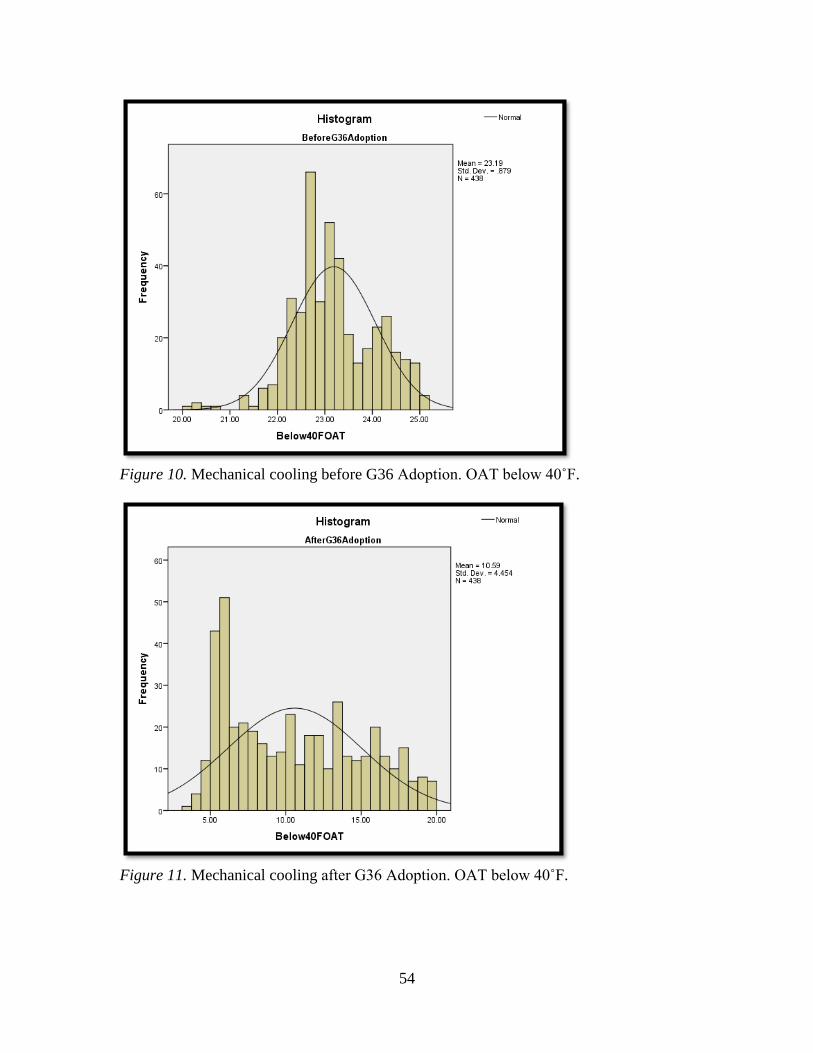
54
Figure 10. Mechanical cooling before G36 Adoption. OAT below 40˚F.
Figure 11. Mechanical cooling after G36 Adoption. OAT below 40˚F.
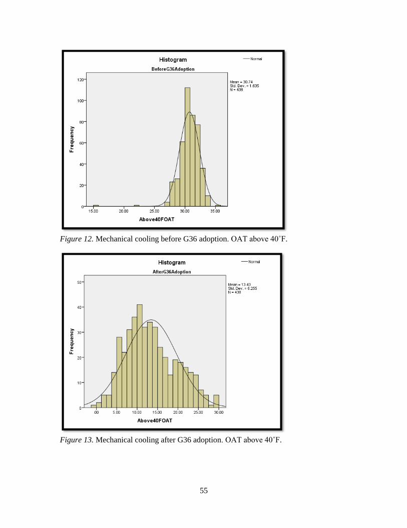
55
Figure 12. Mechanical cooling before G36 adoption. OAT above 40˚F.
Figure 13. Mechanical cooling after G36 adoption. OAT above 40˚F.
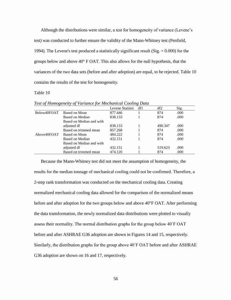
56
Although the distributions were similar, a test for homogeneity of variance (Levene’s
test) was conducted to further ensure the validity of the Mann-Whitney test (Penfield,
1994). The Levene's test produced a statistically significant result (Sig. = 0.000) for the
groups below and above 40° F OAT. This also allows for the null hypothesis, that the
variances of the two data sets (before and after adoption) are equal, to be rejected. Table 10
contains the results of the test for homogeneity.
Table 10
Test of Homogeneity of Variance for Mechanical Cooling Data Levene Statistic df1 df2 Sig.
Below40FOAT Based on Mean 877.446 1 874 .000
Based on Median 838.133 1 874 .000
Based on Median and with
adjusted df 838.133 1 490.347 .000
Based on trimmed mean 857.268 1 874 .000
Above40FOAT Based on Mean 484.222 1 874 .000
Based on Median 432.151 1 874 .000
Based on Median and with
adjusted df 432.151 1 519.623 .000
Based on trimmed mean 474.120 1 874 .000
Because the Mann-Whitney test did not meet the assumption of homogeneity, the
results for the median tonnage of mechanical cooling could not be confirmed. Therefore, a
2-step rank transformation was conducted on the mechanical cooling data. Creating
normalized mechanical cooling data allowed for the comparison of the normalized means
before and after adoption for the two groups below and above 40°F OAT. After performing
the data transformation, the newly normalized data distributions were plotted to visually
assess their normality. The normal distribution graphs for the group below 40˚F OAT
before and after ASHRAE G36 adoption are shown in Figures 14 and 15, respectively.
Similarly, the distribution graphs for the group above 40˚F OAT before and after ASHRAE
G36 adoption are shown on 16 and 17, respectively.
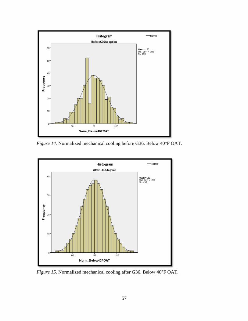
57
Figure 14. Normalized mechanical cooling before G36. Below 40°F OAT.
Figure 15. Normalized mechanical cooling after G36. Below 40°F OAT.
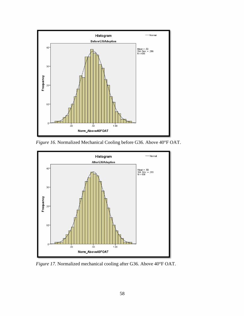
58
Figure 16. Normalized Mechanical Cooling before G36. Above 40°F OAT.
Figure 17. Normalized mechanical cooling after G36. Above 40°F OAT.
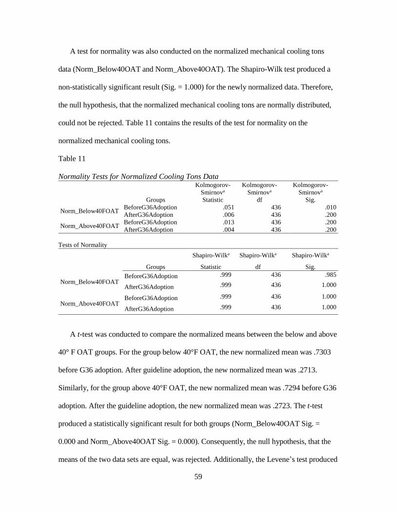
59
A test for normality was also conducted on the normalized mechanical cooling tons
data (Norm_Below40OAT and Norm_Above40OAT). The Shapiro-Wilk test produced a
non-statistically significant result (Sig. = 1.000) for the newly normalized data. Therefore,
the null hypothesis, that the normalized mechanical cooling tons are normally distributed,
could not be rejected. Table 11 contains the results of the test for normality on the
normalized mechanical cooling tons.
Table 11
Normality Tests for Normalized Cooling Tons Data
Groups
Kolmogorov-
Smirnova
Kolmogorov-
Smirnova
Kolmogorov-
Smirnova
Statistic df Sig.
Norm_Below40FOAT BeforeG36Adoption .051 436 .010
AfterG36Adoption .006 436 .200
Norm_Above40FOAT BeforeG36Adoption .013 436 .200
AfterG36Adoption .004 436 .200
Tests of Normality
Groups
Shapiro-Wilka Shapiro-Wilka Shapiro-Wilka
Statistic df Sig.
Norm_Below40FOAT BeforeG36Adoption .999 436 .985
AfterG36Adoption .999 436 1.000
Norm_Above40FOAT BeforeG36Adoption .999 436 1.000
AfterG36Adoption .999 436 1.000
A t-test was conducted to compare the normalized means between the below and above
40° F OAT groups. For the group below 40°F OAT, the new normalized mean was .7303
before G36 adoption. After guideline adoption, the new normalized mean was .2713.
Similarly, for the group above 40°F OAT, the new normalized mean was .7294 before G36
adoption. After the guideline adoption, the new normalized mean was .2723. The t-test
produced a statistically significant result for both groups (Norm_Below40OAT Sig. =
0.000 and Norm_Above40OAT Sig. = 0.000). Consequently, the null hypothesis, that the
means of the two data sets are equal, was rejected. Additionally, the Levene’s test produced
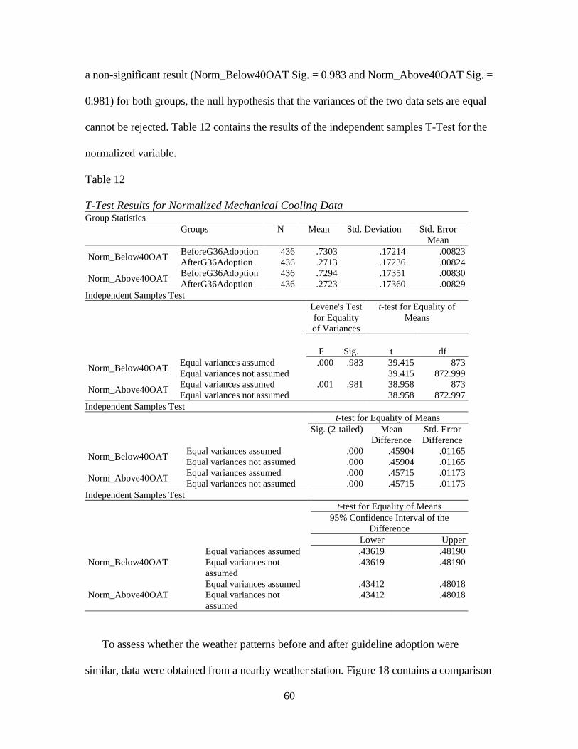
60
a non-significant result (Norm_Below40OAT Sig. = 0.983 and Norm_Above40OAT Sig. =
0.981) for both groups, the null hypothesis that the variances of the two data sets are equal
cannot be rejected. Table 12 contains the results of the independent samples T-Test for the
normalized variable.
Table 12
T-Test Results for Normalized Mechanical Cooling Data Group Statistics
Groups N Mean Std. Deviation Std. Error
Mean
Norm_Below40OAT BeforeG36Adoption 436 .7303 .17214 .00823
AfterG36Adoption 436 .2713 .17236 .00824
Norm_Above40OAT BeforeG36Adoption 436 .7294 .17351 .00830
AfterG36Adoption 436 .2723 .17360 .00829
Independent Samples Test
Levene's Test
for Equality
of Variances
t-test for Equality of
Means
F Sig. t df
Norm_Below40OAT Equal variances assumed .000 .983 39.415 873
Equal variances not assumed 39.415 872.999
Norm_Above40OAT Equal variances assumed .001 .981 38.958 873
Equal variances not assumed 38.958 872.997
Independent Samples Test
t-test for Equality of Means
Sig. (2-tailed) Mean
Difference
Std. Error
Difference
Norm_Below40OAT Equal variances assumed .000 .45904 .01165
Equal variances not assumed .000 .45904 .01165
Norm_Above40OAT Equal variances assumed .000 .45715 .01173
Equal variances not assumed .000 .45715 .01173
Independent Samples Test
t-test for Equality of Means
95% Confidence Interval of the
Difference
Lower Upper
Norm_Below40OAT
Equal variances assumed .43619 .48190
Equal variances not
assumed
.43619 .48190
Norm_Above40OAT
Equal variances assumed .43412 .48018
Equal variances not
assumed
.43412 .48018
To assess whether the weather patterns before and after guideline adoption were
similar, data were obtained from a nearby weather station. Figure 18 contains a comparison
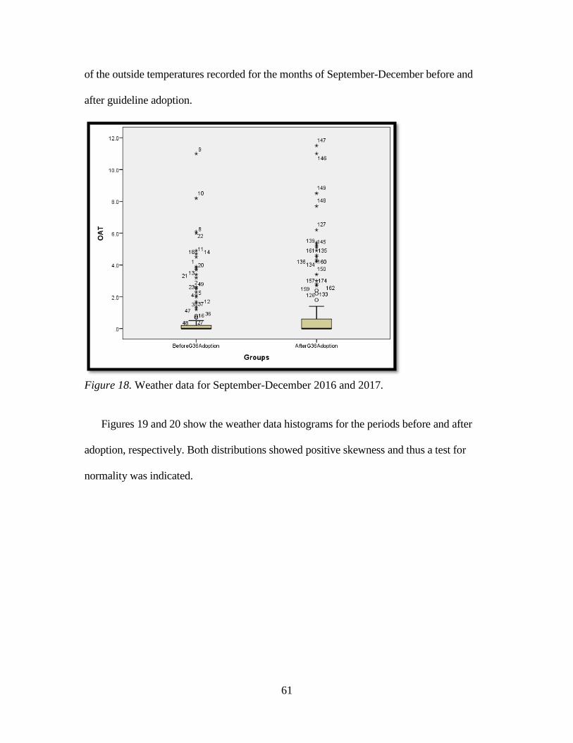
61
of the outside temperatures recorded for the months of September-December before and
after guideline adoption.
Figure 18. Weather data for September-December 2016 and 2017.
Figures 19 and 20 show the weather data histograms for the periods before and after
adoption, respectively. Both distributions showed positive skewness and thus a test for
normality was indicated.
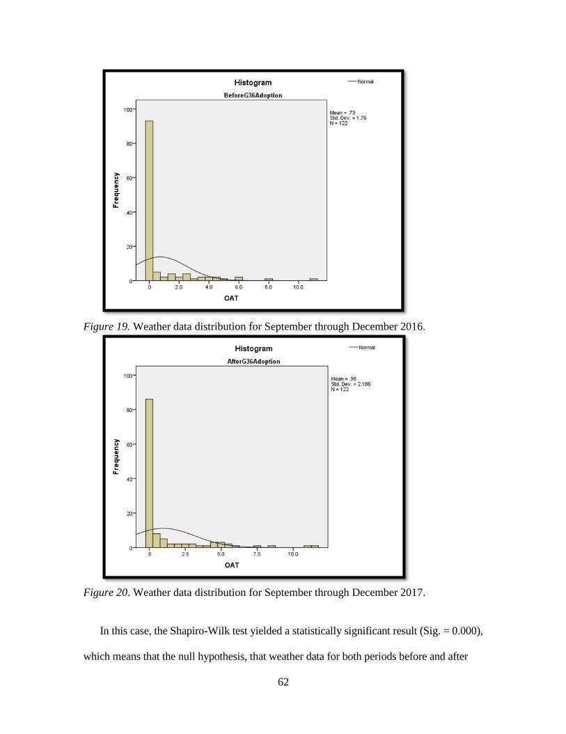
62
Figure 19. Weather data distribution for September through December 2016.
Figure 20. Weather data distribution for September through December 2017.
In this case, the Shapiro-Wilk test yielded a statistically significant result (Sig. = 0.000),
which means that the null hypothesis, that weather data for both periods before and after
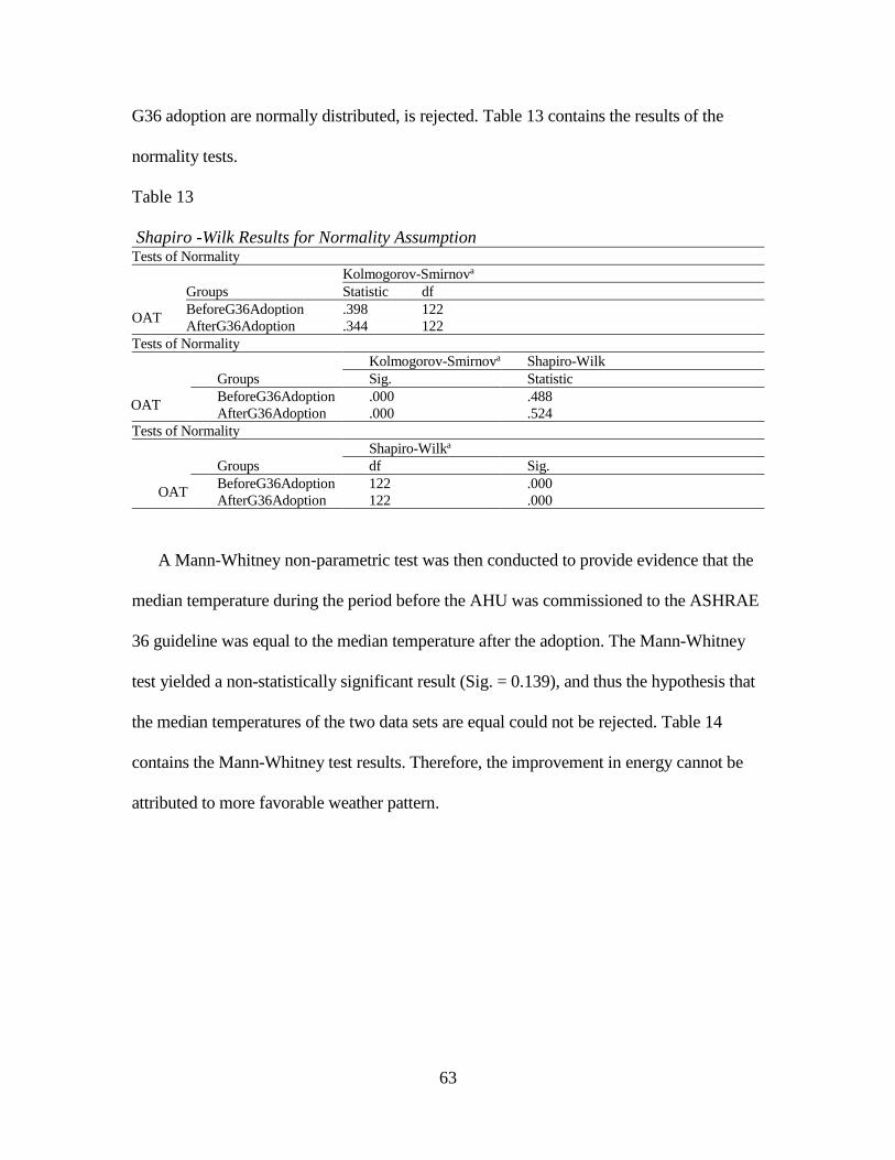
63
G36 adoption are normally distributed, is rejected. Table 13 contains the results of the
normality tests.
Table 13
Shapiro -Wilk Results for Normality Assumption Tests of Normality
Groups
Kolmogorov-Smirnova
Statistic df
OAT BeforeG36Adoption .398 122
AfterG36Adoption .344 122
Tests of Normality
Groups
Kolmogorov-Smirnova Shapiro-Wilk
Sig. Statistic
OAT BeforeG36Adoption .000 .488
AfterG36Adoption .000 .524
Tests of Normality
Groups
Shapiro-Wilka
df Sig.
OAT BeforeG36Adoption 122 .000
AfterG36Adoption 122 .000
A Mann-Whitney non-parametric test was then conducted to provide evidence that the
median temperature during the period before the AHU was commissioned to the ASHRAE
36 guideline was equal to the median temperature after the adoption. The Mann-Whitney
test yielded a non-statistically significant result (Sig. = 0.139), and thus the hypothesis that
the median temperatures of the two data sets are equal could not be rejected. Table 14
contains the Mann-Whitney test results. Therefore, the improvement in energy cannot be
attributed to more favorable weather pattern.
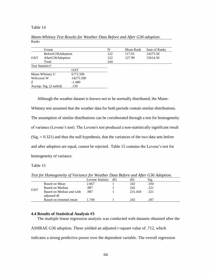
64
Table 14
Mann-Whitney Test Results for Weather Data Before and After G36 adoption. Ranks
Group N Mean Rank Sum of Ranks
OAT
BeforeG36Adoption 122 117.01 14275.50
AfterG36Adoption 122 127.99 15614.50
Total 244
Test Statisticsa OAT
Mann-Whitney U 6772.500
Wilcoxon W 14275.500
Z -1.480
Asymp. Sig. (2-tailed) .139
Although the weather dataset is known not to be normally distributed, the Mann-
Whitney test assumed that the weather data for both periods contain similar distributions.
The assumption of similar distributions can be corroborated through a test for homogeneity
of variance (Levene’s test). The Levene's test produced a non-statistically significant result
(Sig. = 0.321) and thus the null hypothesis, that the variances of the two data sets before
and after adoption are equal, cannot be rejected. Table 15 contains the Levene’s test for
homogeneity of variance.
Table 15
Test for Homogeneity of Variance for Weather Data Before and After G36 Adoption. Levene Statistic df1 df2 Sig.
OAT
Based on Mean 2.667 1 242 .104
Based on Median .987 1 242 .321
Based on Median and with
adjusted df
.987 1 231.434 .321
Based on trimmed mean 1.749 1 242 .187
4.4 Results of Statistical Analysis #3
The multiple linear regression analysis was conducted with datasets obtained after the
ASHRAE G36 adoption. These yielded an adjusted r-square value of .712, which
indicates a strong predictive power over the dependent variable. The overall regression
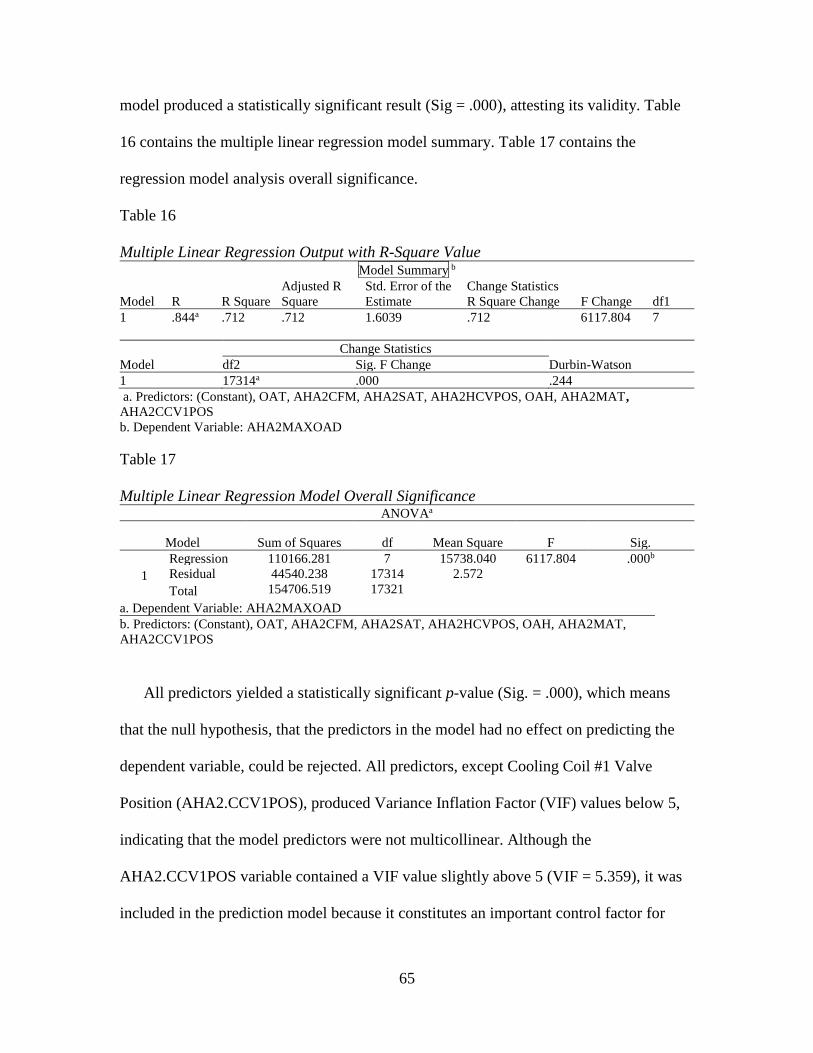
65
model produced a statistically significant result (Sig = .000), attesting its validity. Table
16 contains the multiple linear regression model summary. Table 17 contains the
regression model analysis overall significance.
Table 16
Multiple Linear Regression Output with R-Square Value Model Summary b
Model R R Square
Adjusted R
Square
Std. Error of the
Estimate
Change Statistics
R Square Change F Change df1
1 .844a .712 .712 1.6039 .712 6117.804 7
Model
Change Statistics
Durbin-Watson df2 Sig. F Change
1 17314a .000 .244
a. Predictors: (Constant), OAT, AHA2CFM, AHA2SAT, AHA2HCVPOS, OAH, AHA2MAT,
AHA2CCV1POS
b. Dependent Variable: AHA2MAXOAD
Table 17
Multiple Linear Regression Model Overall Significance ANOVAa
Model Sum of Squares df Mean Square F Sig.
1
Regression 110166.281 7 15738.040 6117.804 .000b
Residual 44540.238 17314 2.572
Total 154706.519 17321
a. Dependent Variable: AHA2MAXOAD
b. Predictors: (Constant), OAT, AHA2CFM, AHA2SAT, AHA2HCVPOS, OAH, AHA2MAT,
AHA2CCV1POS
All predictors yielded a statistically significant p-value (Sig. = .000), which means
that the null hypothesis, that the predictors in the model had no effect on predicting the
dependent variable, could be rejected. All predictors, except Cooling Coil #1 Valve
Position (AHA2.CCV1POS), produced Variance Inflation Factor (VIF) values below 5,
indicating that the model predictors were not multicollinear. Although the
AHA2.CCV1POS variable contained a VIF value slightly above 5 (VIF = 5.359), it was
included in the prediction model because it constitutes an important control factor for
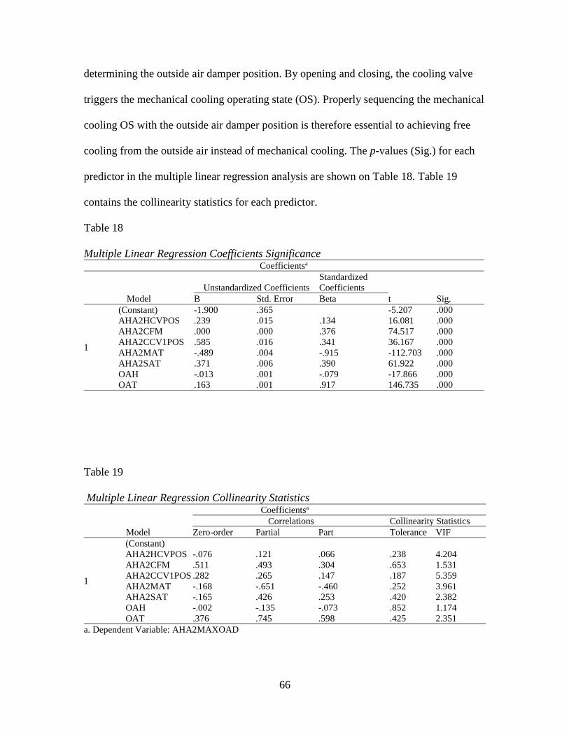
66
determining the outside air damper position. By opening and closing, the cooling valve
triggers the mechanical cooling operating state (OS). Properly sequencing the mechanical
cooling OS with the outside air damper position is therefore essential to achieving free
cooling from the outside air instead of mechanical cooling. The p-values (Sig.) for each
predictor in the multiple linear regression analysis are shown on Table 18. Table 19
contains the collinearity statistics for each predictor.
Table 18
Multiple Linear Regression Coefficients Significance Coefficientsa
Model
Unstandardized Coefficients
Standardized
Coefficients
t Sig. B Std. Error Beta
1
(Constant) -1.900 .365 -5.207 .000
AHA2HCVPOS .239 .015 .134 16.081 .000
AHA2CFM .000 .000 .376 74.517 .000
AHA2CCV1POS .585 .016 .341 36.167 .000
AHA2MAT -.489 .004 -.915 -112.703 .000
AHA2SAT .371 .006 .390 61.922 .000
OAH -.013 .001 -.079 -17.866 .000
OAT .163 .001 .917 146.735 .000
Table 19
Multiple Linear Regression Collinearity Statistics Coefficientsa
Model
Correlations Collinearity Statistics
Zero-order Partial Part Tolerance VIF
1
(Constant)
AHA2HCVPOS -.076 .121 .066 .238 4.204
AHA2CFM .511 .493 .304 .653 1.531
AHA2CCV1POS .282 .265 .147 .187 5.359
AHA2MAT -.168 -.651 -.460 .252 3.961
AHA2SAT -.165 .426 .253 .420 2.382
OAH -.002 -.135 -.073 .852 1.174
OAT .376 .745 .598 .425 2.351
a. Dependent Variable: AHA2MAXOAD
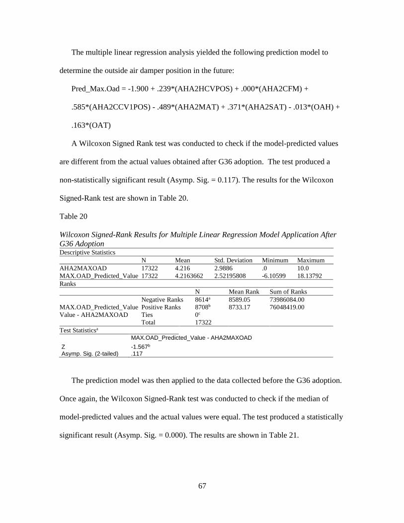
67
The multiple linear regression analysis yielded the following prediction model to
determine the outside air damper position in the future:
Pred_Max.Oad = -1.900 + .239*(AHA2HCVPOS) + .000*(AHA2CFM) +
.585*(AHA2CCV1POS) - .489*(AHA2MAT) + .371*(AHA2SAT) - .013*(OAH) +
.163*(OAT)
A Wilcoxon Signed Rank test was conducted to check if the model-predicted values
are different from the actual values obtained after G36 adoption. The test produced a
non-statistically significant result (Asymp. Sig. = 0.117). The results for the Wilcoxon
Signed-Rank test are shown in Table 20.
Table 20
Wilcoxon Signed-Rank Results for Multiple Linear Regression Model Application After
G36 Adoption Descriptive Statistics N Mean Std. Deviation Minimum Maximum
AHA2MAXOAD 17322 4.216 2.9886 .0 10.0
MAX.OAD_Predicted_Value 17322 4.2163662 2.52195808 -6.10599 18.13792
Ranks N Mean Rank Sum of Ranks
MAX.OAD_Predicted_Value
Value - AHA2MAXOAD
Negative Ranks 8614a 8589.05 73986084.00
Positive Ranks 8708b 8733.17 76048419.00
Ties 0c
Total 17322
Test Statisticsa
MAX.OAD_Predicted_Value - AHA2MAXOAD
Z -1.567b Asymp. Sig. (2-tailed) .117
The prediction model was then applied to the data collected before the G36 adoption.
Once again, the Wilcoxon Signed-Rank test was conducted to check if the median of
model-predicted values and the actual values were equal. The test produced a statistically
significant result (Asymp. Sig. = 0.000). The results are shown in Table 21.
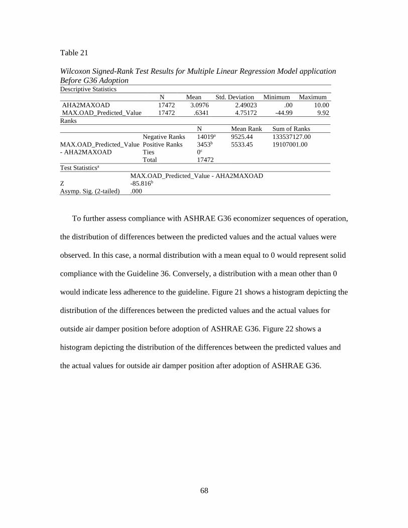
68
Table 21
Wilcoxon Signed-Rank Test Results for Multiple Linear Regression Model application
Before G36 Adoption Descriptive Statistics
N Mean Std. Deviation Minimum Maximum
AHA2MAXOAD 17472 3.0976 2.49023 .00 10.00
MAX.OAD_Predicted_Value 17472 .6341 4.75172 -44.99 9.92
Ranks N Mean Rank Sum of Ranks
MAX.OAD_Predicted_Value
- AHA2MAXOAD
Negative Ranks 14019a 9525.44 133537127.00
Positive Ranks 3453b 5533.45 19107001.00
Ties 0c
Total 17472
Test Statisticsa MAX.OAD_Predicted_Value - AHA2MAXOAD
Z -85.816b
Asymp. Sig. (2-tailed) .000
To further assess compliance with ASHRAE G36 economizer sequences of operation,
the distribution of differences between the predicted values and the actual values were
observed. In this case, a normal distribution with a mean equal to 0 would represent solid
compliance with the Guideline 36. Conversely, a distribution with a mean other than 0
would indicate less adherence to the guideline. Figure 21 shows a histogram depicting the
distribution of the differences between the predicted values and the actual values for
outside air damper position before adoption of ASHRAE G36. Figure 22 shows a
histogram depicting the distribution of the differences between the predicted values and
the actual values for outside air damper position after adoption of ASHRAE G36.
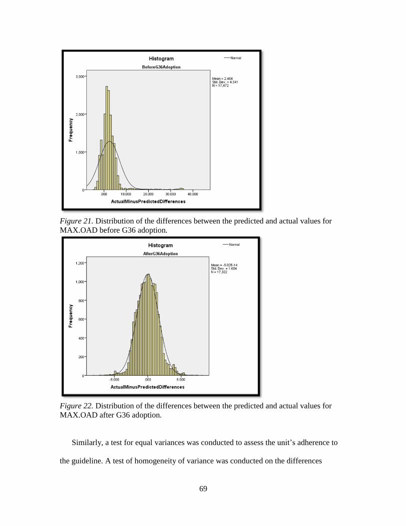
69
Figure 21. Distribution of the differences between the predicted and actual values for
MAX.OAD before G36 adoption.
Figure 22. Distribution of the differences between the predicted and actual values for
MAX.OAD after G36 adoption.
Similarly, a test for equal variances was conducted to assess the unit’s adherence to
the guideline. A test of homogeneity of variance was conducted on the differences
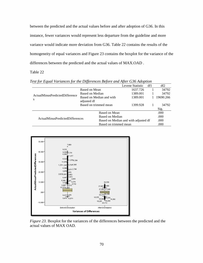
70
between the predicted and the actual values before and after adoption of G36. In this
instance, fewer variances would represent less departure from the guideline and more
variance would indicate more deviation from G36. Table 22 contains the results of the
homogeneity of equal variances and Figure 23 contains the boxplot for the variance of the
differences between the predicted and the actual values of MAX.OAD .
Table 22
Test for Equal Variances for the Differences Before and After G36 Adoption Levene Statistic df1 df2
ActualMinusPredictedDifference
s
Based on Mean 1637.726 1 34792
Based on Median 1389.001 1 34792
Based on Median and with
adjusted df
1389.001 1 19690.266
Based on trimmed mean 1399.928 1 34792
Sig.
ActualMinusPredictedDifferences
Based on Mean .000
Based on Median .000
Based on Median and with adjusted df .000
Based on trimmed mean .000
Figure 23. Boxplot for the variances of the differences between the predicted and the
actual values of MAX OAD.
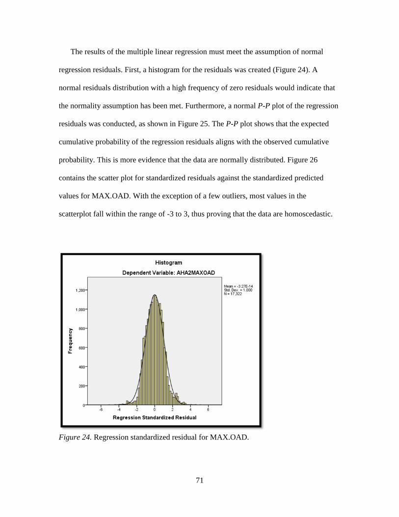
71
The results of the multiple linear regression must meet the assumption of normal
regression residuals. First, a histogram for the residuals was created (Figure 24). A
normal residuals distribution with a high frequency of zero residuals would indicate that
the normality assumption has been met. Furthermore, a normal P-P plot of the regression
residuals was conducted, as shown in Figure 25. The P-P plot shows that the expected
cumulative probability of the regression residuals aligns with the observed cumulative
probability. This is more evidence that the data are normally distributed. Figure 26
contains the scatter plot for standardized residuals against the standardized predicted
values for MAX.OAD. With the exception of a few outliers, most values in the
scatterplot fall within the range of -3 to 3, thus proving that the data are homoscedastic.
Figure 24. Regression standardized residual for MAX.OAD.
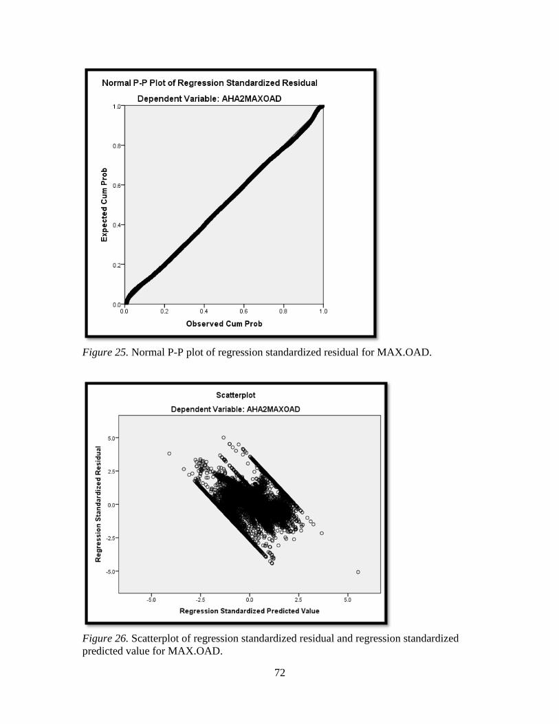
72
Figure 25. Normal P-P plot of regression standardized residual for MAX.OAD.
Figure 26. Scatterplot of regression standardized residual and regression standardized
predicted value for MAX.OAD.
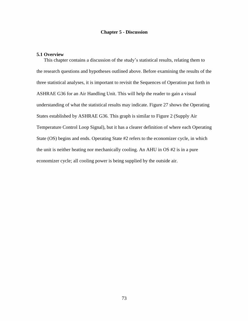
73
Chapter 5 - Discussion
5.1 Overview
This chapter contains a discussion of the study’s statistical results, relating them to
the research questions and hypotheses outlined above. Before examining the results of the
three statistical analyses, it is important to revisit the Sequences of Operation put forth in
ASHRAE G36 for an Air Handling Unit. This will help the reader to gain a visual
understanding of what the statistical results may indicate. Figure 27 shows the Operating
States established by ASHRAE G36. This graph is similar to Figure 2 (Supply Air
Temperature Control Loop Signal), but it has a clearer definition of where each Operating
State (OS) begins and ends. Operating State #2 refers to the economizer cycle, in which
the unit is neither heating nor mechanically cooling. An AHU in OS #2 is in a pure
economizer cycle; all cooling power is being supplied by the outside air.

74
Figure 27. Multiple zone AHUs operating states. ©ASHRAE www.ashrae.org High-performance sequences of operations for HVAC Systems, 2018.
Figures 28 and 29 show a scatter plot of the AHU operational data before and after
the system was commissioned to comply with the ASHRAE G36. In both Figures 28 and
29, the red data points represent the heating coil valve position with respect to the outside
air when the unit is in a heating operating cycle. The heating coil valve is closed when it
is at the 0 position. The heating coil pattern shown in Figures 28 and 29 is different from
the one shown Figure 20 because the heating coil valves are reverse-acting: the valves are
fully closed when they are at or near the 10 position. The green data points represent the
outside air damper (OAD) position. The dark blue data points represent the cooling coil
valve 1 position with respect to the outside air. The light blue data points represent
cooling coil valve 2. Depending on the geographical location of the unit, a second cooling
coil is sometimes utilized to maximize the AHU’s cooling capability.
Before the adoption of ASHRAE G36, the AHU used in this study exhibited a pattern
that did not clearly define where each OS started or ended. In fact, the unit did not
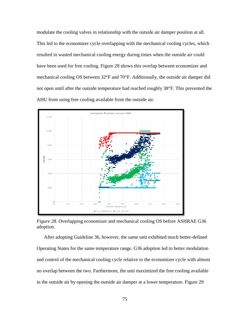
75
modulate the cooling valves in relationship with the outside air damper position at all.
This led to the economizer cycle overlapping with the mechanical cooling cycles, which
resulted in wasted mechanical cooling energy during times when the outside air could
have been used for free cooling. Figure 28 shows this overlap between economizer and
mechanical cooling OS between 32°F and 70°F. Additionally, the outside air damper did
not open until after the outside temperature had reached roughly 38°F. This prevented the
AHU from using free cooling available from the outside air.
Figure 28. Overlapping economizer and mechanical cooling OS before ASHRAE G36
adoption.
After adopting Guideline 36, however, the same unit exhibited much better-defined
Operating States for the same temperature range. G36 adoption led to better modulation
and control of the mechanical cooling cycle relative to the economizer cycle with almost
no overlap between the two. Furthermore, the unit maximized the free cooling available
in the outside air by opening the outside air damper at a lower temperature. Figure 29
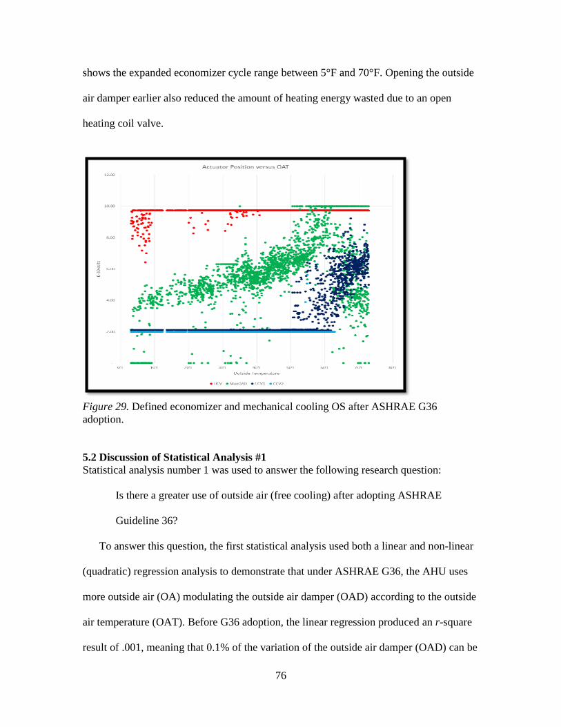
76
shows the expanded economizer cycle range between 5°F and 70°F. Opening the outside
air damper earlier also reduced the amount of heating energy wasted due to an open
heating coil valve.
Figure 29. Defined economizer and mechanical cooling OS after ASHRAE G36
adoption.
5.2 Discussion of Statistical Analysis #1
Statistical analysis number 1 was used to answer the following research question:
Is there a greater use of outside air (free cooling) after adopting ASHRAE
Guideline 36?
To answer this question, the first statistical analysis used both a linear and non-linear
(quadratic) regression analysis to demonstrate that under ASHRAE G36, the AHU uses
more outside air (OA) modulating the outside air damper (OAD) according to the outside
air temperature (OAT). Before G36 adoption, the linear regression produced an r-square
result of .001, meaning that 0.1% of the variation of the outside air damper (OAD) can be
77
explained by the variation of outside air temperature (OAT). The quadratic regression
results produced an r-square of .044, which indicates that only 4.4% of the OAD’s
variation can be explained by the OAT. This result also indicated that there was no linear
relationship between the two. In other words, the linear and quadratic models have almost
no predictive power over the OAD position when using the OAT as a predictor.
After G36 adoption, however, the linear regression results produced an r-square of
.721, which indicates that 72.1% of the variation in the OAD can be explained by
variation in OAT. This linear result was significant, so a linear regression model could be
trusted to have enough predictive power over the outside air damper position when using
the outside air temperature as a predictor. The quadratic regression after ASHRAE G36
adoption produced an r-square value of .814. A higher r-square means that the quadratic
model produced the equation that best fit the dataset. Both the linear and the quadratic
results indicate that the adoption of ASHRAE Guideline 36 does lead to higher utilization
of outside air.
5.3 Discussion of Statistical Analysis #2
With statistical analysis 2, this study aimed to answer the following research question:
Is there a difference in energy use for building cooling before and after adoption
of ASHRAE Guideline 36?
To answer this question, the data were divided based on the outdoor temperature
method for economizer savings calculations. According to this method, economizer
savings are calculated in two steps, when the OAT is below 40°F and when it is above
40°F. For OATs below 40°F, the median mechanical cooling tons produced by the air
handler before G36 adoption were 23.07. After G36 adoption, the median mechanical
cooling tons were 10.27. When the OAT was above 40°F, the median mechanical cooling
78
tons produced by the air handler before G36 adoption were 30.70 and 12.59 after G36
adoption. This result equates to roughly a 43% energy savings for a single AHU in one
winter season after being commissioned per ASHRAE Guideline 36.
For the non-normalized mechanical cooling data, the Mann-Whitney test produced a
statistically significant result (Sig. = 0.000) for both groups below and above 40°F OAT.
However, since the Mann-Whitney did not meet the assumption of homogeneity, a 2-step
rank transformation and a subsequent independent samples T-Test were conducted on the
normalized mechanical cooling data. This provided further evidence that there was a
difference in mechanical cooling usage before and after G36 adoption. The new
normalized mechanical cooling data met the assumption of normality, producing a
statistically significant Shapiro-Wilk Test result for the periods before and after the
adoption of ASHRAE G36. Additionally, the Independent Samples T-Test conducted on
the new normalized mechanical cooling data produced statistically significant results
(Sig. = 0.000) for both groups below and above 40°F OAT, thus confirming the median
figures for mechanical cooling tonnage.
Furthermore, the Mann-Whitney test conducted on the weather data for the months of
September-December demonstrated that both selected periods in 2016 and 2017 had
similar weather patterns. Both periods had a median temperature of 0.000°F, meaning
that there was the same amount of available outside air free cooling before and after the
guideline adoption. Commissioning the AHU per Guideline 36 resulted in less use of
mechanical cooling by the unit, so more outside air was utilized for free cooling.
Therefore, the results of the statistical analysis 2 confirm the research hypothesis that the
adoption of ASHRAE Guideline 36 does lead to higher energy efficiency. Additionally,
79
research question number 2 can be answered positively: there is a difference in energy
use before and after adoption of ASHRAE G36.
5.4 Discussion of Statistical Analysis #3
The aim of statistical analysis 3 was to produce a multiple linear regression model to
answer the following research question:
Can a model be developed to let building owners know whether the AHU system
is working in compliance with ASHRAE Guideline 36 as it relates to
economizer/free cooling sequences of operations?
The multiple linear regression analysis conducted after the G36 adoption produced an
adjusted r-square value of .712. All predictors used in the multiple linear regression were
statistically significant with a P-Value of .000. While predictors with VIFs values above
5 may not be practical in multiple linear regression analysis, they were essential to the
accuracy of the prediction model in this case study.
The multiple linear regression model was applied to the data obtained after G36
adoption using the Wilcoxon-Signed Rank test. The Wilcoxon Signed-Rank test
produced a test statistic result of .177, which was not statistically significant. Therefore,
the null hypothesis, that the median OAD values predicted by model and the actual OAD
values after G36 adoption are equal (mean differences equal 0), was not rejected.
After the model was verified, it was then applied to the data from before the adoption
of G36 to check if a statistical difference existed between the values predicted by the
model and the actual values obtained before the guideline implementations. This was also
tested using the Wilcoxon Signed Rank test. The Wilcoxon-Signed Rank test produced a
statistically significant result of 0.000. Therefore, this study rejects the null hypothesis
that the median values for the OAD position results predicted by the model and the actual
80
OAD positions are equal. The results of the prediction model allow for a positive answer
to research question number 3: a model has, in fact, been developed to inform building
owners about AHU adherence to the economizer cycle (free cooling) per ASHRAE G36.
Because the model determines the correct position of the outside air damper given
certain conditions (outside air temperature, position of the heating and cooling valves,
mixed air temperature, etc.) a building owner can use the model to predict the correct
position of the outside air damper for any given AHU in different weather environments.
If the AHU’s outside air damper position is different from the model’s prediction, that
may be an indication that the AHU is malfunctioning or that the unit is no longer
operating as specified by ASHRAE G36.
Figure 21 and 22, which show the differences between the values predicted by the
model and the actual values before and after G36 adoption, shows a greater dispersion
before ASHRAE G36 adoption. This suggests less compliance with ASHRAE G36
sequences of operations for economizer cycles. Similarly, Figure 23 shows visually that
the variances of the differences are much worse before the ASHRAE Guideline 36 were
adopted, also indicating that the AHU departed from its intended operation according to
the guideline. Therefore, the third hypothesis proposed in this study, that a prediction
model will provide insights as to whether an economizer sequence of operation is
properly performing, was validated.
81
Chapter 6 – Conclusions
6.1 Research Contributions
The chief contributions of this study to the HVAC industry are a timeline and
framework for building owners that are considering adopting Guideline 36. Figure 30
contains a G36 implementation timeline for both new and existing buildings. For a new
building, there are 4 main steps to implementing Guideline 36:
1. Design systems with Sequences of Operations based on G36 (Design phase)
2. Collect data from the building automation system (Commissioning phase).
3. Gather operational data for at least one year (Operation phase).
4. Use data analytics to ensure continuity of the building systems operation per
ASHRAE G36 over time (Implementation phase)
For existing buildings, ASHRAE G36 adoption may begin with the Operation phase of
the timeline.
Figure 31 depicts a framework for building owners to use to determine whether the
economizer sequence is optimized according to Guideline 36. To ensure maximum
Outside Air usage, the framework focuses on predicting the position of the Outside Air
Damper using several predictor variables. Although predictors may change depending on
specific situations and geographical locations, the framework does provide examples of
possible predictor. For implementation in both new and existing buildings, understanding
weather patterns is extremely important. With existing buildings, weather patterns can be
compared against historical records. The first operation phase of new buildings can serve
as benchmark for future comparisons.
82
Although the G36 adoption timeline and economizer optimization framework are
important to the HVAC industry, the study’s main point of interest for building owners is
the ability to track their Return on Investment (ROI). The optimization framework uses a
standard improvement threshold of 25% for economizer savings in order to determine if
further implementation is warranted. However, different situations may dictate different
thresholds. Giving accurate information to building owners about initial implementation
costs and possible energy savings after adopting G36 can help them make wise business
decisions about Guideline 36. One important aspect of the savings resulting from G36
implementation is that they may continue for many years. However, a building’s facilities
manager must continue using the steps in the optimization framework for performance
tracking. Any deviation from previous savings could indicate system malfunction,
weather-related issues, or scheduled system shutdowns and power outages.
A major goal of this study is to highlight the benefits of implementing G36
throughout an entire building complex. The framework put forth in this study focused on
the economizer cycles for Multizone Air Handling Units because of their high cost of
operation. However, many types of AHUs are covered by the guideline, including Single
Zone Variable Air Volume AHUs and Dual Fan/Dual Duct Heating Variable Air Volume
AHUs. G36 offers specific sequences of operation for each of these unit types.
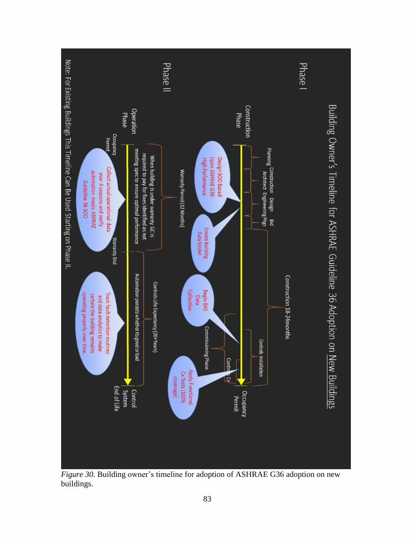
83
Figure 30. Building owner’s timeline for adoption of ASHRAE G36 adoption on new
buildings.
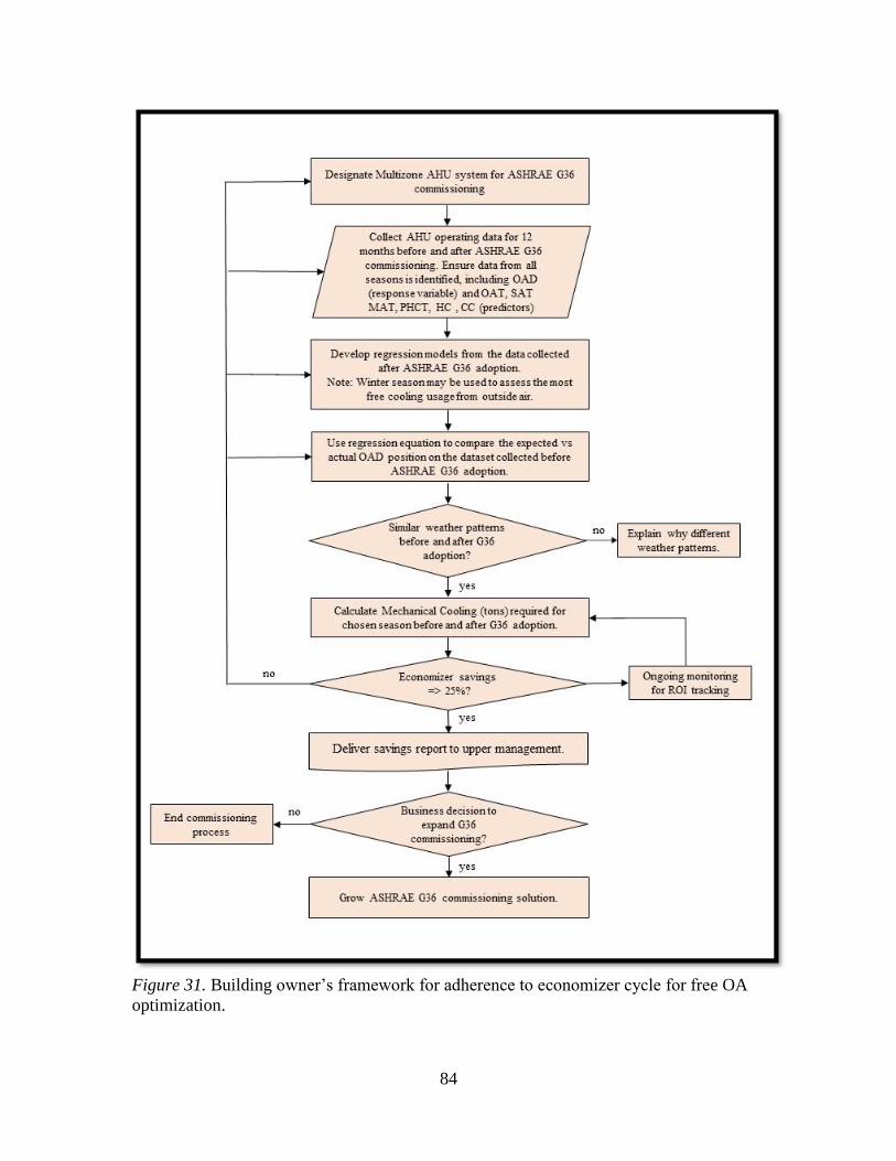
84
Figure 31. Building owner’s framework for adherence to economizer cycle for free OA
optimization.
85
6.1.1 Case Study
Since expanding the implementation of G36 is the goal of this study, another AHU in
the same building was examined to demonstrate that using the framework for building
owners can provide insights about the current AHU operations. The framework was
followed step by step. First, an air handler was selected. Air Handler 09 (AHA09) is
similar to AHA02 in that it serves a variety of spaces with different uses, and it must
calculate how much fresh air (outside air) is needed to serve all occupied spaces. Data
was then collected from AHA09 in the winter season from September 1, 2018 to
November 10, 2018.
A linear regression analysis of the outside air and the outside air handler was then
performed. The linear regression produced an adjusted r-square value of .138, showing
that less than 14% of the modulation of the outside air damper could be attributed to a
change in the outside air temperature. The G36 multiple linear regression model created
in this study was applied to the data collected from AHA09. This model predicted the
position for the outside air damper if AHA09 had adhered to ASHRAE G36. A Wilcoxon
Signed Rank test was performed. This test was used because the differences between the
predicted position of the outside air damper and its actual position values were not
normally distributed (Kolmogorov-Smirnov test for normality, Sig. = 0.000). The
Wilcoxon Signed Rank produced a statistically significant result (Asymp. Sig. = 0.000),
eliminating the possibility that differences of the median predicted values and the actual
OAD values equals 0.
The next step in the framework calls for weather normalization analysis. Using
weather data from the nearest airport, weather patterns from 2017 were compared with
the ongoing 2018 winter season. In both winter seasons, the median temperature was
86
0.000°F. A test of homogeneity of variance conducted on this data for both years
produced a non-statistically significant result, showing that the weather distributions,
although not normally distributed, were similar to each other.
When mechanical cooling calculations were conducted according to step 6 of the
framework, they demonstrated that the unit was not operating according to ASHRAE
G36 and therefore was not using the outside air for free cooling in the most efficient way
possible. For example, for the periods AHA09 used a median usage of 21.64 tons of
mechanical cooling when the outside air temperature (OAT) was below 40°F and 20.76
tons when the OAT was above 40°F. These results are similar to those obtained from unit
AHA02 prior to commissioning it with Guideline 36. Given that winter 2017 and 2018
had similar weather patterns, it is safe to say that unit AHA09 is not as not currently
optimized for outside air usage. Following the building owner framework for all AHUs in
the building may allow the owner to see inefficiencies in different AHUs in order to
make a business decision about improving energy savings.
6.2 Future Research
Guideline 36 covers sequences of operation for Variable Air Volume (VAV) systems
only, but the guideline is not static. Instead, it is a living document that will be improved
upon over time. One possible area for further improvement is adding sequences of
operation for enthalpy wheels. Enthalpy wheels recover cooling energy from exhaust
systems and recycle it into supply systems. This reduces mechanical cooling loads and
theoretically saves energy. While this study focuses on the application of ASHRAE
Guideline 36 to improve energy efficiency through an improved economizer cycle that uses
more outside air for free cooling, enthalpy wheels may also assist in providing free cooling
that would otherwise be wasted. Similarly, desiccant wheels, a type of enthalpy wheel that
87
reduces the amount of moisture in the return air, lower the cooling load on the VAV’s
cooling coils when the mechanical cooling cycle is activated.
In the future, ASHRAE intends to expand Guideline 36 to create high-performance
sequences for Dedicated Outdoor Air Systems (DOAS) (Hydeman et al., 2015). DOAS are
usually very inefficient because they require complex sequences of operations (Fernandez,
N., Katipamula, S., & Underhill, R., 2017). A DOAS also typically uses enthalpy wheels,
and properly controlling these wheels is essential to their efficiency. Currently, enthalpy
wheels are used more often in European countries and the northeastern part of the U.S., but
there is an opportunity to expand these systems to other regions within the U.S. Such an
expansion may require manufacturers to adopt advanced sequences of operation so that
field installation is less troublesome (Hydeman et al., 2015).
6.3 Conclusions
The main purpose of this study was to address the problem of effectively using outside
air for free cooling. Although many commissioning procedures currently exist for ensuring
that AHUs adhere to their intended designs, this study provided evidence that ASHRAE
Guideline 36 is the only method that solves the problem at the design level. ASHRAE G36
provides a high-performing sequence of operations for AHUs that all HVAC design
engineers can implement in order to reduce HVAC operational costs.
The quantitative analyses performed in this study provided empirical evidence for the
claim of ASHRAE G36’s effectiveness. The linear regression analysis showed that more
outside air was used after ASHRAE Guideline 36 was implemented. This study also
demonstrated that greater use of outside air for free cooling led to improved energy
efficiency because the HVAC unit needed to use less mechanical cooling.
88
In terms of practical applications, the study contains a model that building owners can
use to confirm Guideline 36 compliance. Results from the study also allowed for the
creation of a timeline and framework for building owners who are considering adopting
Guideline 36 in their buildings and ensuring AHU economizer optimization. Implementing
ASHRAE Guideline 36 and following the G36 timeline and validation framework may
have a national impact on energy use, lowering costs and reducing the carbon footprint of
buildings with complex HVAC systems.
89
References
AABC Commissioning Group. (2005). ACG commissioning guideline. Washington,
D.C.: AABC Commissioning Group.
Aktacir, M. A., Büyükalaca, O., & Yılmaz, T. (2006). Life-cycle cost analysis for
constant-air-volume and variable-air-volume air-conditioning systems. Applied
Energy, 83(6), 606-627.
Alves, O., Monteiro, E., Brito, P., & Romano, P. (2016). Measurement and classification
of energy efficiency in HVAC systems. Energy and Buildings, 130, 408-419. doi:
10.1016/j.enbuild.2016.08.070
American Society of Heating, Refrigerating, and Air-Conditioning Engineers
(ASHRAE). (2018, June 4). ASHRAE guideline 36-2018: High performance
sequences of operations for HVAC systems. Atlanta, GA: ASHRAE.
ASHRAE (2017). Titles, purposes, and scopes. Ashrae.org. Retrieved from
https://www.ashrae.org/standards-research--technology/standards--
guidelines/titles-purposes-and-scopes#gpc36p
ASHRAE. (2015). 43: HVAC Commissioning. In ASHRAE handbook: Heating,
ventilating, and air-conditioning applications (SI Edition). American Society of
Heating, Refrigerating and Air-Conditioning Engineers, Inc.
Beil, I., Hiskens, I., & Backhaus, S. (2016). Frequency regulation from commercial
building HVAC demand response. Proceedings of the IEEE, 104(4), 745-757.
doi: 10.1109/JPROC.2016.2520640
90
Borrego, M., Douglas, E. P., & Amelink, C. T. (2009). Quantitative, qualitative, and
mixed research methods in engineering education. Journal of Engineering
Education, 98(1), 53-66.
Capehart, B. L., & Brambley, M. R. (2015). Automated diagnostics and analytics for
buildings. Lilburn, GA: Fairmont Press.
Cetin, K. S., & Kallus, C. (2016). Data-driven methodology for energy and peak load
reduction of residential HVAC systems. Procedia Engineering, 145, 852-859.
Chandel, S. S., Sharma, A., & Marwaha, B. M. (2016). Review of energy efficiency
initiatives and regulations for residential buildings in India. Renewable and
Sustainable Energy Reviews, 54, 1443-1458. doi: 10.1016/j.rser.2015.10.060
Chatterjee, S., & Hadi, A. S. (2015). Regression analysis by example. John Wiley &
Sons.
Cho, Young-Hum., & Liu, Mingsheng. (2010). Improving energy efficiency with the
various control sequences for VAV systems through continuous commissioning.
International Journal of Energy Research, 34, 1291-1301.
Daly, D., Cooper, P., & Ma, Z. (2014). Understanding the risks and uncertainties
introduced by common assumptions in energy simulations for Australian
commercial buildings. Energy and Buildings, 75, 382-393. doi:
10.1016/j.enbuild.2014.02.028
Deru, M. P., Deru, M. P., & Kelsey, J. (2011). Procedures for commercial building
energy audits. American Society of Heating, Refrigerating, and Air-Conditioning
Engineers.
91
Douglas A. Penfield (1994). Choosing a Two-Sample Location Test. The Journal of
Experimental Education, 62:4, 343-360. doi: 10.1080/00220973.1994.9944139
Du, Z., Jin, X., Fang, X., & Fan, B. (2016). A dual-benchmark based energy analysis
method to evaluate control strategies for building HVAC systems. Applied
Energy, 183, 700-714. doi: 10.1016/j.apenergy.2016.09.019
Fernandez, N., Katipamula, S., & Underhill, R. (2017). Optimizing control of dedicated
outdoor air systems with energy recovery in commercial buildings. Journal of
Energy Engineering, 143(1).
Ghahramani, A., Jazizadeh, F., & Becerik-Gerber, B. (2014). A knowledge based
approach for selecting energy-aware and comfort-driven HVAC temperature set
points. Energy and Buildings, 85, 536-548. doi: 10.1016/j.enbuild.2014.09.055
Gupton Jr, W. (2001). HVAC controls: Operation and maintenance. Fairmont Press.
Hydeman, M., Taylor, S. T., & Eubanks, B. (2015). Control sequences and controller
programming. ASHRAE Journal., 57(3), 58–62.
Interval Data Systems, Inc. (2018, 10 15). why-buildings-inefficient. Retrieved from
Interval Data Systems: http://intdatsys.com
Jackson, Barbara J. (2010) Construction management jumpstart: The best first step
toward a career in construction management. Wiley Publishing, Inc.
Johnson, B. (2001). Toward a new classification of nonexperimental quantitative
research. Educational Researcher, 30(2), 3-13.
Kubba, S. (2012). . Handbook of green building design and construction: LEED,
BREEAM, and Green Globes. Boston, MA : Butterworth-Heinemann.
92
Lee, S. H., Hong, T., Piette, M. A., Sawaya, G., Chen, Y., & Taylor-Lange, S. C. (2015).
Accelerating the energy retrofit of commercial buildings using a database of
energy efficiency performance. Energy, 90, 738-747. doi:
10.1016/j.energy.2015.07.107
Marino, C., Minichiello, F., & Bahnfleth, W. (2015). The influence of surface finishes on
the energy demand of HVAC systems for existing buildings. Energy and
Buildings, 95, 70-79. doi: 10.1016/j.enbuild.2015.02.036
Mendoza-Serrano, D. I., & Chmielewski, D. J. (2015). Smart grid coordination in
building HVAC systems: Computational efficiency of constrained economic
linear optimal control. Science and Technology for the Built Environment, 21(6),
812-823. doi: 10.1080/23744731.2015.1057059
Merriam, S. B., & Tisdell, E. J. (2015). Qualitative research: A guide to design and
implementation. John Wiley & Sons.
Pearson, R. W. (2009). Statistical persuasion: How to collect, analyze, and present data
accurately, honestly, and persuasively. Sage Publications.
Pritoni, M., Salmon, K., Sanguinetti, A., Morejohn, J., & Modera, M. (2017). Occupant
thermal feedback for improved efficiency in university buildings. Energy and
Buildings, 144, 241-250.
Robinson, Tony. (2014). 5.4.2 RCx Process. In High-performance buildings: A guide for
owners & managers. Fairmont Press, Inc.
Ruparathna, R., Hewage, K., & Sadiq, R. (2016). Improving the energy efficiency of the
existing building stock: A critical review of commercial and institutional
93
buildings. Renewable and Sustainable Energy Reviews, 53, 1032-1045. doi:
10.1016/j.rser.2015.09.084
Shah, H. (2015) A guide to the engineering management body of knowledge (4th Edition).
Rolla, MO: American Society for Engineering Management.
Sun, Z., Li, L., & Dababneh, F. (2016). Plant-level electricity demand response for
combined manufacturing system and heating, venting, and air-conditioning
(HVAC) systems. Journal of Cleaner Production, 135, 1650-1657.
Tabachnick, B. G., & Fidell, L. S. (2007). Using multivariate statistics. Allyn &
Bacon/Pearson Education.
Taylor, S. T., & Cheng, C. H. (2010). Why enthalpy economizers don’t work. ASHRAE
Journal, 52(11), 12-28.
Templeton, G. F. (2011). A two-step approach for transforming continuous variables to
normal: implications and recommendations for IS research. CAIS, 28(1), 41-58.
Thumann, Albert Niehus, Terry Younger, William J. (2013). 17.1 Retro-Commissioning
(RCx) Defined. In Handbook of energy audits (9th Ed) pp. 451,453. Fairmont
Press, Inc.
Tukur, A. G. (2016). Reducing airflow energy use in multiple zone VAV systems
(Doctoral dissertation). University of Dayton).
Turner, W. C., & Doty, S. (2013). Energy management handbook. Lilburn, GA: The
Fairmont Press, Inc.
U.S. Environmental Protection Agency (2001). Guide to industrial assessments for
pollution prevention and energy efficiency. Washington, D.C.: U.S.
Environmental Protection Agency Office of Research and Development.
94
Vakiloroaya, V., Samali, B., Fakhar, A., & Pishghadam, K. (2014). A review of different
strategies for HVAC energy saving. Energy Conversion and Management, 77,
738-754.
Wang, Z., Ding, Y., Geng, G., & Zhu, N. (2014). Analysis of energy efficiency retrofit
schemes for heating, ventilating and air-conditioning systems in existing office
buildings based on the modified bin method. Energy Conversion and
Management, 77, 233-242. doi: 10.1016/j.enconman.2013.09.037
Wendes, H. (1994). Variable air volume manual. The Fairmont Press.
Whitman, B., Johnson, B., Tomczyk, J., & Silberstein, E. (2012). Refrigeration and air
conditioning technology. Cengage Learning.
Yang, Z., & Becerik-Gerber, B. (2016). How does building occupancy influence energy
efficiency of HVAC systems? Energy Procedia, 88, 775-780.
Yang, Z., Ghahramani, A., & Becerik-Gerber, B. (2016). Building occupancy diversity
and HVAC (heating, ventilation, and air conditioning) system energy efficiency.
Energy, 109, 641-649. doi: 10.1016/j.energy.2016.04.099
Zaatari, M., Novoselac, A., & Siegel, J. (2014). The relationship between filter pressure
drop, indoor air quality, and energy consumption in rooftop HVAC units.
Building and Environment, 73, 151-161. doi: 10.1016/j.buildenv.2013.12.010
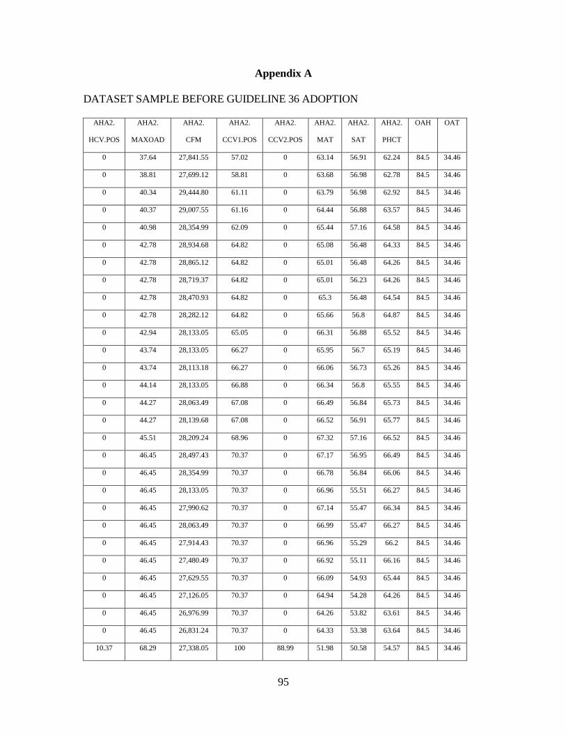
95
Appendix A
DATASET SAMPLE BEFORE GUIDELINE 36 ADOPTION
AHA2.
HCV.POS
AHA2.
MAXOAD
AHA2.
CFM
AHA2.
CCV1.POS
AHA2.
CCV2.POS
AHA2.
MAT
AHA2.
SAT
AHA2.
PHCT
OAH OAT
0 37.64 27,841.55 57.02 0 63.14 56.91 62.24 84.5 34.46
0 38.81 27,699.12 58.81 0 63.68 56.98 62.78 84.5 34.46
0 40.34 29,444.80 61.11 0 63.79 56.98 62.92 84.5 34.46
0 40.37 29,007.55 61.16 0 64.44 56.88 63.57 84.5 34.46
0 40.98 28,354.99 62.09 0 65.44 57.16 64.58 84.5 34.46
0 42.78 28,934.68 64.82 0 65.08 56.48 64.33 84.5 34.46
0 42.78 28,865.12 64.82 0 65.01 56.48 64.26 84.5 34.46
0 42.78 28,719.37 64.82 0 65.01 56.23 64.26 84.5 34.46
0 42.78 28,470.93 64.82 0 65.3 56.48 64.54 84.5 34.46
0 42.78 28,282.12 64.82 0 65.66 56.8 64.87 84.5 34.46
0 42.94 28,133.05 65.05 0 66.31 56.88 65.52 84.5 34.46
0 43.74 28,133.05 66.27 0 65.95 56.7 65.19 84.5 34.46
0 43.74 28,113.18 66.27 0 66.06 56.73 65.26 84.5 34.46
0 44.14 28,133.05 66.88 0 66.34 56.8 65.55 84.5 34.46
0 44.27 28,063.49 67.08 0 66.49 56.84 65.73 84.5 34.46
0 44.27 28,139.68 67.08 0 66.52 56.91 65.77 84.5 34.46
0 45.51 28,209.24 68.96 0 67.32 57.16 66.52 84.5 34.46
0 46.45 28,497.43 70.37 0 67.17 56.95 66.49 84.5 34.46
0 46.45 28,354.99 70.37 0 66.78 56.84 66.06 84.5 34.46
0 46.45 28,133.05 70.37 0 66.96 55.51 66.27 84.5 34.46
0 46.45 27,990.62 70.37 0 67.14 55.47 66.34 84.5 34.46
0 46.45 28,063.49 70.37 0 66.99 55.47 66.27 84.5 34.46
0 46.45 27,914.43 70.37 0 66.96 55.29 66.2 84.5 34.46
0 46.45 27,480.49 70.37 0 66.92 55.11 66.16 84.5 34.46
0 46.45 27,629.55 70.37 0 66.09 54.93 65.44 84.5 34.46
0 46.45 27,126.05 70.37 0 64.94 54.28 64.26 84.5 34.46
0 46.45 26,976.99 70.37 0 64.26 53.82 63.61 84.5 34.46
0 46.45 26,831.24 70.37 0 64.33 53.38 63.64 84.5 34.46
10.37 68.29 27,338.05 100 88.99 51.98 50.58 54.57 84.5 34.46
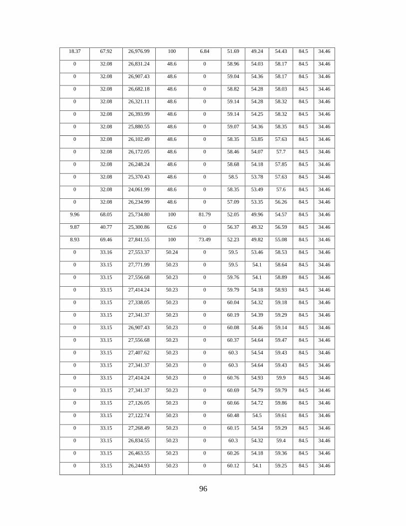
96
18.37 67.92 26,976.99 100 6.84 51.69 49.24 54.43 84.5 34.46
0 32.08 26,831.24 48.6 0 58.96 54.03 58.17 84.5 34.46
0 32.08 26,907.43 48.6 0 59.04 54.36 58.17 84.5 34.46
0 32.08 26,682.18 48.6 0 58.82 54.28 58.03 84.5 34.46
0 32.08 26,321.11 48.6 0 59.14 54.28 58.32 84.5 34.46
0 32.08 26,393.99 48.6 0 59.14 54.25 58.32 84.5 34.46
0 32.08 25,880.55 48.6 0 59.07 54.36 58.35 84.5 34.46
0 32.08 26,102.49 48.6 0 58.35 53.85 57.63 84.5 34.46
0 32.08 26,172.05 48.6 0 58.46 54.07 57.7 84.5 34.46
0 32.08 26,248.24 48.6 0 58.68 54.18 57.85 84.5 34.46
0 32.08 25,370.43 48.6 0 58.5 53.78 57.63 84.5 34.46
0 32.08 24,061.99 48.6 0 58.35 53.49 57.6 84.5 34.46
0 32.08 26,234.99 48.6 0 57.09 53.35 56.26 84.5 34.46
9.96 68.05 25,734.80 100 81.79 52.05 49.96 54.57 84.5 34.46
9.87 40.77 25,300.86 62.6 0 56.37 49.32 56.59 84.5 34.46
8.93 69.46 27,841.55 100 73.49 52.23 49.82 55.08 84.5 34.46
0 33.16 27,553.37 50.24 0 59.5 53.46 58.53 84.5 34.46
0 33.15 27,771.99 50.23 0 59.5 54.1 58.64 84.5 34.46
0 33.15 27,556.68 50.23 0 59.76 54.1 58.89 84.5 34.46
0 33.15 27,414.24 50.23 0 59.79 54.18 58.93 84.5 34.46
0 33.15 27,338.05 50.23 0 60.04 54.32 59.18 84.5 34.46
0 33.15 27,341.37 50.23 0 60.19 54.39 59.29 84.5 34.46
0 33.15 26,907.43 50.23 0 60.08 54.46 59.14 84.5 34.46
0 33.15 27,556.68 50.23 0 60.37 54.64 59.47 84.5 34.46
0 33.15 27,407.62 50.23 0 60.3 54.54 59.43 84.5 34.46
0 33.15 27,341.37 50.23 0 60.3 54.64 59.43 84.5 34.46
0 33.15 27,414.24 50.23 0 60.76 54.93 59.9 84.5 34.46
0 33.15 27,341.37 50.23 0 60.69 54.79 59.79 84.5 34.46
0 33.15 27,126.05 50.23 0 60.66 54.72 59.86 84.5 34.46
0 33.15 27,122.74 50.23 0 60.48 54.5 59.61 84.5 34.46
0 33.15 27,268.49 50.23 0 60.15 54.54 59.29 84.5 34.46
0 33.15 26,834.55 50.23 0 60.3 54.32 59.4 84.5 34.46
0 33.15 26,463.55 50.23 0 60.26 54.18 59.36 84.5 34.46
0 33.15 26,244.93 50.23 0 60.12 54.1 59.25 84.5 34.46
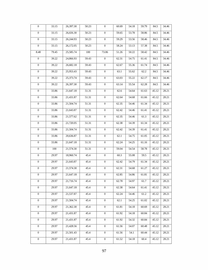
97
0 33.15 26,397.30 50.23 0 60.69 54.18 59.79 84.5 34.46
0 33.15 26,026.30 50.23 0 59.65 53.78 58.86 84.5 34.46
0 33.15 26,244.93 50.23 0 59.29 53.56 58.46 84.5 34.46
0 33.15 26,172.05 50.23 0 58.24 53.13 57.38 84.5 34.46
8.48 79.45 25,585.74 100 73.06 51.26 50.22 58.42 84.5 34.46
0 39.22 24,866.93 59.43 0 62.31 54.75 61.41 84.5 34.46
0 39.22 26,682.18 59.43 0 62.67 55.36 61.74 84.5 34.46
0 39.22 25,953.43 59.43 0 63.1 55.62 62.2 84.5 34.46
0 39.22 25,373.74 59.43 0 63.03 55.22 62.17 84.5 34.46
0 39.22 26,397.30 59.43 0 63.14 55.54 62.28 84.5 34.46
0 33.86 21,647.18 51.31 0 62.6 54.64 61.63 45.12 28.21
0 33.86 21,431.87 51.31 0 62.64 54.68 61.66 45.12 28.21
0 33.86 21,504.74 51.31 0 62.35 54.46 61.34 45.12 28.21
0 33.86 21,643.87 51.31 0 62.42 54.46 61.41 45.12 28.21
0 33.86 21,577.62 51.31 0 62.35 54.46 61.3 45.12 28.21
0 33.86 21,720.05 51.31 0 62.38 54.39 61.34 45.12 28.21
0 33.86 21,504.74 51.31 0 62.42 54.39 61.41 45.12 28.21
0 33.86 20,636.87 51.31 0 62.1 54.75 61.05 45.12 28.21
0 33.86 21,647.18 51.31 0 62.24 54.25 61.16 45.12 28.21
0 100 21,574.30 51.31 0 59.04 54.54 58.78 45.12 28.21
0 29.97 18,960.74 45.4 0 60.3 55.08 59.5 45.12 28.21
0 29.97 21,643.87 45.4 0 62.42 54.79 61.34 45.12 28.21
0 29.97 21,574.30 45.4 0 62.31 54.68 61.27 45.12 28.21
0 29.97 21,647.18 45.4 0 62.85 54.86 61.81 45.12 28.21
0 29.97 21,716.74 45.4 0 62.78 54.97 61.7 45.12 28.21
0 29.97 21,647.18 45.4 0 62.38 54.64 61.41 45.12 28.21
0 29.97 21,537.87 45.4 0 62.24 54.46 61.2 45.12 28.21
0 29.97 21,504.74 45.4 0 62.1 54.25 61.02 45.12 28.21
0 29.97 21,362.30 45.4 0 61.81 54.18 60.69 45.12 28.21
0 29.97 21,431.87 45.4 0 61.92 54.18 60.84 45.12 28.21
0 29.97 21,431.87 45.4 0 61.92 54.32 60.84 45.12 28.21
0 29.97 21,428.56 45.4 0 61.56 54.07 60.48 45.12 28.21
0 29.97 21,501.43 45.4 0 61.56 54.1 60.44 45.12 28.21
0 29.97 21,431.87 45.4 0 61.52 54.18 60.4 45.12 28.21
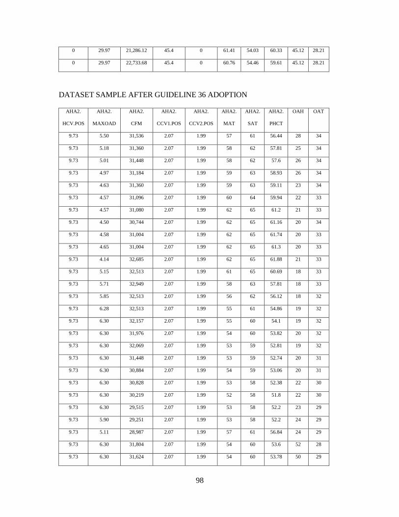
98
0 29.97 21,286.12 45.4 0 61.41 54.03 60.33 45.12 28.21
0 29.97 22,733.68 45.4 0 60.76 54.46 59.61 45.12 28.21
DATASET SAMPLE AFTER GUIDELINE 36 ADOPTION
AHA2.
HCV.POS
AHA2.
MAXOAD
AHA2.
CFM
AHA2.
CCV1.POS
AHA2.
CCV2.POS
AHA2.
MAT
AHA2.
SAT
AHA2.
PHCT
OAH OAT
9.73 5.50 31,536 2.07 1.99 57 61 56.44 28 34
9.73 5.18 31,360 2.07 1.99 58 62 57.81 25 34
9.73 5.01 31,448 2.07 1.99 58 62 57.6 26 34
9.73 4.97 31,184 2.07 1.99 59 63 58.93 26 34
9.73 4.63 31,360 2.07 1.99 59 63 59.11 23 34
9.73 4.57 31,096 2.07 1.99 60 64 59.94 22 33
9.73 4.57 31,080 2.07 1.99 62 65 61.2 21 33
9.73 4.50 30,744 2.07 1.99 62 65 61.16 20 34
9.73 4.58 31,004 2.07 1.99 62 65 61.74 20 33
9.73 4.65 31,004 2.07 1.99 62 65 61.3 20 33
9.73 4.14 32,685 2.07 1.99 62 65 61.88 21 33
9.73 5.15 32,513 2.07 1.99 61 65 60.69 18 33
9.73 5.71 32,949 2.07 1.99 58 63 57.81 18 33
9.73 5.85 32,513 2.07 1.99 56 62 56.12 18 32
9.73 6.28 32,513 2.07 1.99 55 61 54.86 19 32
9.73 6.30 32,157 2.07 1.99 55 60 54.1 19 32
9.73 6.30 31,976 2.07 1.99 54 60 53.82 20 32
9.73 6.30 32,069 2.07 1.99 53 59 52.81 19 32
9.73 6.30 31,448 2.07 1.99 53 59 52.74 20 31
9.73 6.30 30,884 2.07 1.99 54 59 53.06 20 31
9.73 6.30 30,828 2.07 1.99 53 58 52.38 22 30
9.73 6.30 30,219 2.07 1.99 52 58 51.8 22 30
9.73 6.30 29,515 2.07 1.99 53 58 52.2 23 29
9.73 5.90 29,251 2.07 1.99 53 58 52.2 24 29
9.73 5.11 28,987 2.07 1.99 57 61 56.84 24 29
9.73 6.30 31,804 2.07 1.99 54 60 53.6 52 28
9.73 6.30 31,624 2.07 1.99 54 60 53.78 50 29
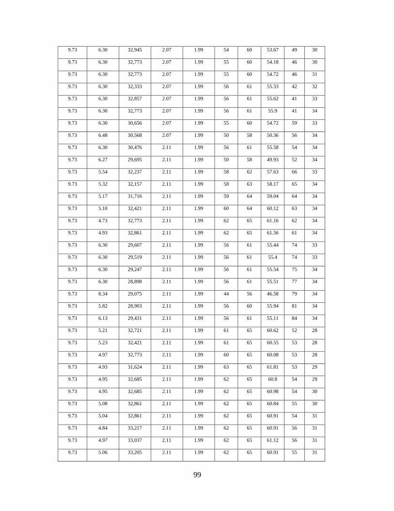
99
9.73 6.30 32,945 2.07 1.99 54 60 53.67 49 30
9.73 6.30 32,773 2.07 1.99 55 60 54.18 46 30
9.73 6.30 32,773 2.07 1.99 55 60 54.72 46 31
9.73 6.30 32,333 2.07 1.99 56 61 55.33 42 32
9.73 6.30 32,857 2.07 1.99 56 61 55.62 41 33
9.73 6.30 32,773 2.07 1.99 56 61 55.9 41 34
9.73 6.30 30,656 2.07 1.99 55 60 54.72 59 33
9.73 6.48 30,568 2.07 1.99 50 58 50.36 56 34
9.73 6.30 30,476 2.11 1.99 56 61 55.58 54 34
9.73 6.27 29,695 2.11 1.99 50 58 49.93 52 34
9.73 5.54 32,237 2.11 1.99 58 62 57.63 66 33
9.73 5.32 32,157 2.11 1.99 58 63 58.17 65 34
9.73 5.17 31,716 2.11 1.99 59 64 59.04 64 34
9.73 5.10 32,421 2.11 1.99 60 64 60.12 63 34
9.73 4.73 32,773 2.11 1.99 62 65 61.16 62 34
9.73 4.93 32,861 2.11 1.99 62 65 61.56 61 34
9.73 6.30 29,607 2.11 1.99 56 61 55.44 74 33
9.73 6.30 29,519 2.11 1.99 56 61 55.4 74 33
9.73 6.30 29,247 2.11 1.99 56 61 55.54 75 34
9.73 6.30 28,898 2.11 1.99 56 61 55.51 77 34
9.73 8.34 29,075 2.11 1.99 44 56 46.58 79 34
9.73 5.82 28,903 2.11 1.99 56 60 55.94 81 34
9.73 6.13 29,431 2.11 1.99 56 61 55.11 84 34
9.73 5.21 32,721 2.11 1.99 61 65 60.62 52 28
9.73 5.23 32,421 2.11 1.99 61 65 60.55 53 28
9.73 4.97 32,773 2.11 1.99 60 65 60.08 53 28
9.73 4.93 31,624 2.11 1.99 63 65 61.81 53 29
9.73 4.95 32,685 2.11 1.99 62 65 60.8 54 29
9.73 4.95 32,685 2.11 1.99 62 65 60.98 54 30
9.73 5.08 32,861 2.11 1.99 62 65 60.84 55 30
9.73 5.04 32,861 2.11 1.99 62 65 60.91 54 31
9.73 4.84 33,217 2.11 1.99 62 65 60.91 56 31
9.73 4.97 33,037 2.11 1.99 62 65 61.12 56 31
9.73 5.06 33,205 2.11 1.99 62 65 60.91 55 31
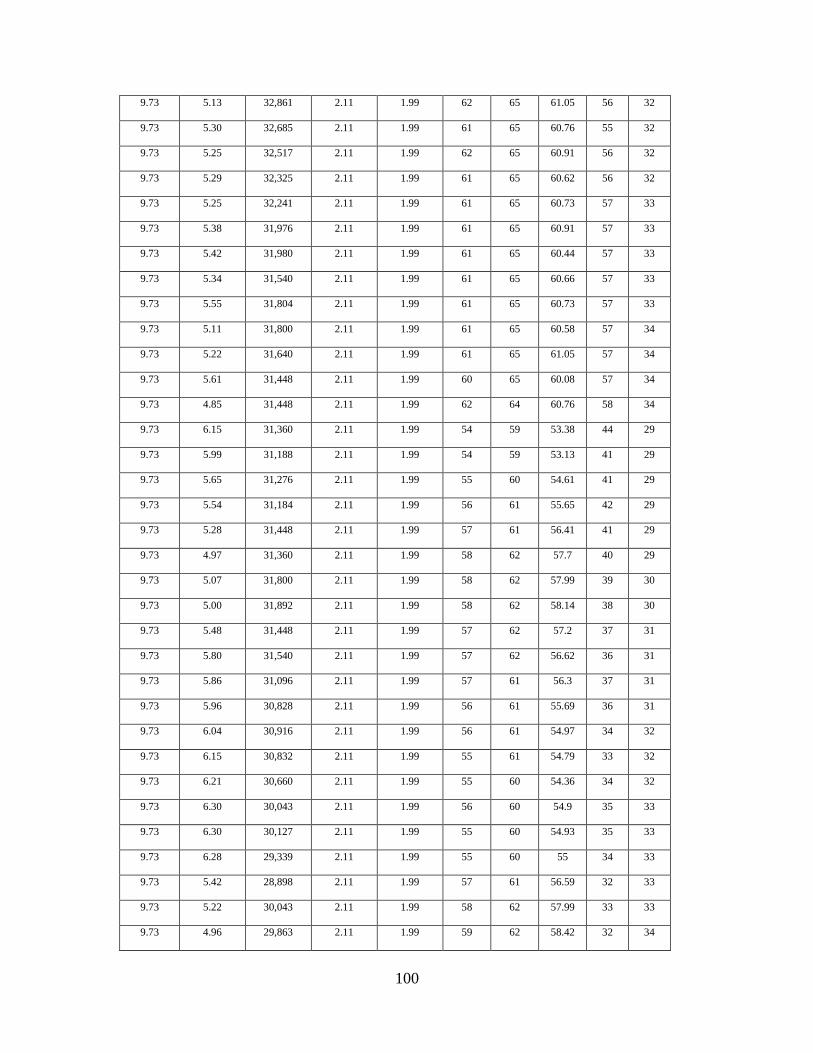
100
9.73 5.13 32,861 2.11 1.99 62 65 61.05 56 32
9.73 5.30 32,685 2.11 1.99 61 65 60.76 55 32
9.73 5.25 32,517 2.11 1.99 62 65 60.91 56 32
9.73 5.29 32,325 2.11 1.99 61 65 60.62 56 32
9.73 5.25 32,241 2.11 1.99 61 65 60.73 57 33
9.73 5.38 31,976 2.11 1.99 61 65 60.91 57 33
9.73 5.42 31,980 2.11 1.99 61 65 60.44 57 33
9.73 5.34 31,540 2.11 1.99 61 65 60.66 57 33
9.73 5.55 31,804 2.11 1.99 61 65 60.73 57 33
9.73 5.11 31,800 2.11 1.99 61 65 60.58 57 34
9.73 5.22 31,640 2.11 1.99 61 65 61.05 57 34
9.73 5.61 31,448 2.11 1.99 60 65 60.08 57 34
9.73 4.85 31,448 2.11 1.99 62 64 60.76 58 34
9.73 6.15 31,360 2.11 1.99 54 59 53.38 44 29
9.73 5.99 31,188 2.11 1.99 54 59 53.13 41 29
9.73 5.65 31,276 2.11 1.99 55 60 54.61 41 29
9.73 5.54 31,184 2.11 1.99 56 61 55.65 42 29
9.73 5.28 31,448 2.11 1.99 57 61 56.41 41 29
9.73 4.97 31,360 2.11 1.99 58 62 57.7 40 29
9.73 5.07 31,800 2.11 1.99 58 62 57.99 39 30
9.73 5.00 31,892 2.11 1.99 58 62 58.14 38 30
9.73 5.48 31,448 2.11 1.99 57 62 57.2 37 31
9.73 5.80 31,540 2.11 1.99 57 62 56.62 36 31
9.73 5.86 31,096 2.11 1.99 57 61 56.3 37 31
9.73 5.96 30,828 2.11 1.99 56 61 55.69 36 31
9.73 6.04 30,916 2.11 1.99 56 61 54.97 34 32
9.73 6.15 30,832 2.11 1.99 55 61 54.79 33 32
9.73 6.21 30,660 2.11 1.99 55 60 54.36 34 32
9.73 6.30 30,043 2.11 1.99 56 60 54.9 35 33
9.73 6.30 30,127 2.11 1.99 55 60 54.93 35 33
9.73 6.28 29,339 2.11 1.99 55 60 55 34 33
9.73 5.42 28,898 2.11 1.99 57 61 56.59 32 33
9.73 5.22 30,043 2.11 1.99 58 62 57.99 33 33
9.73 4.96 29,863 2.11 1.99 59 62 58.42 32 34
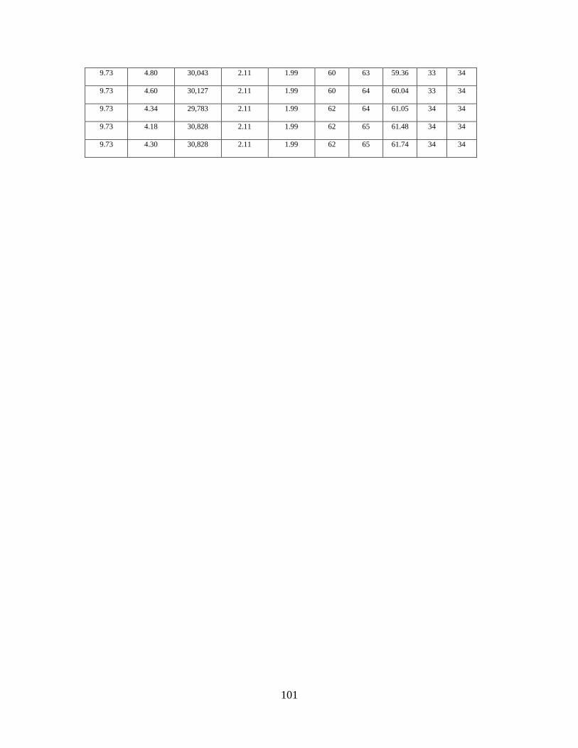
101
9.73 4.80 30,043 2.11 1.99 60 63 59.36 33 34
9.73 4.60 30,127 2.11 1.99 60 64 60.04 33 34
9.73 4.34 29,783 2.11 1.99 62 64 61.05 34 34
9.73 4.18 30,828 2.11 1.99 62 65 61.48 34 34
9.73 4.30 30,828 2.11 1.99 62 65 61.74 34 34
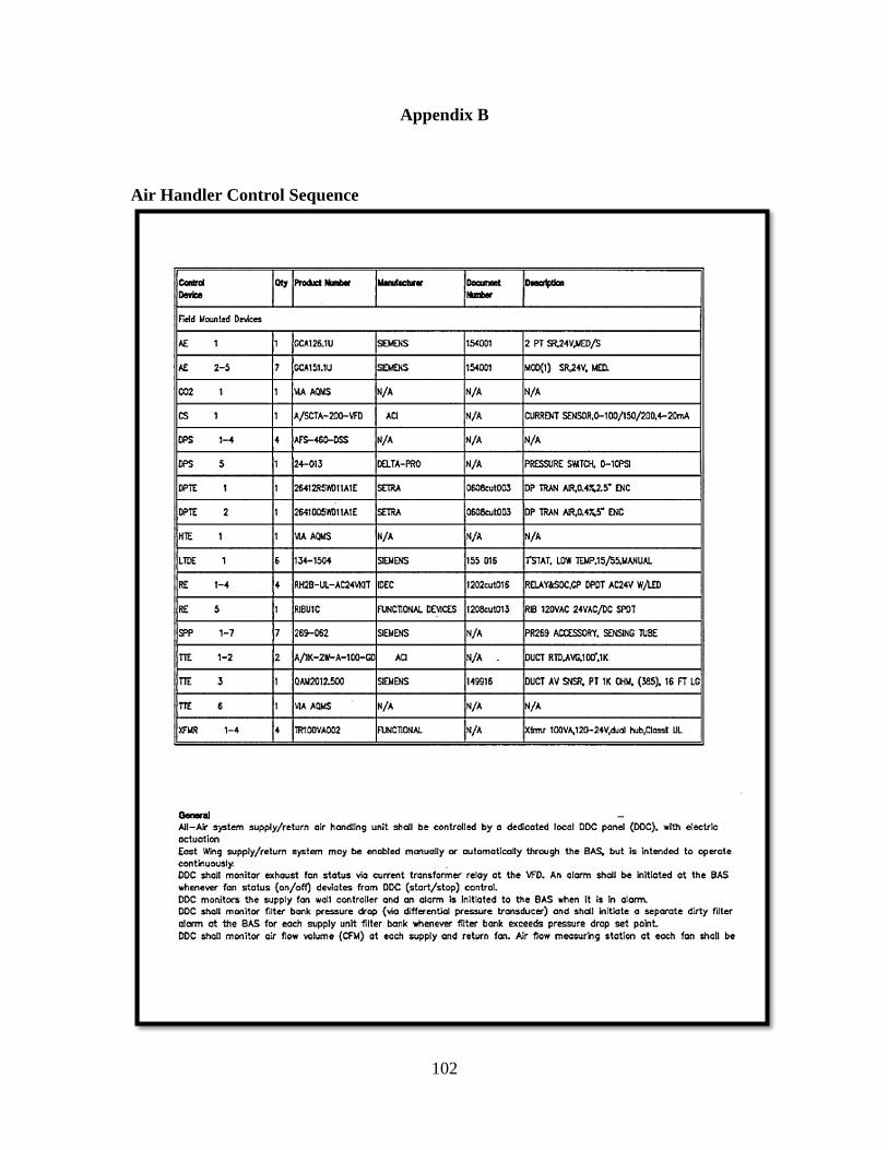
102
Appendix B
Air Handler Control Sequence
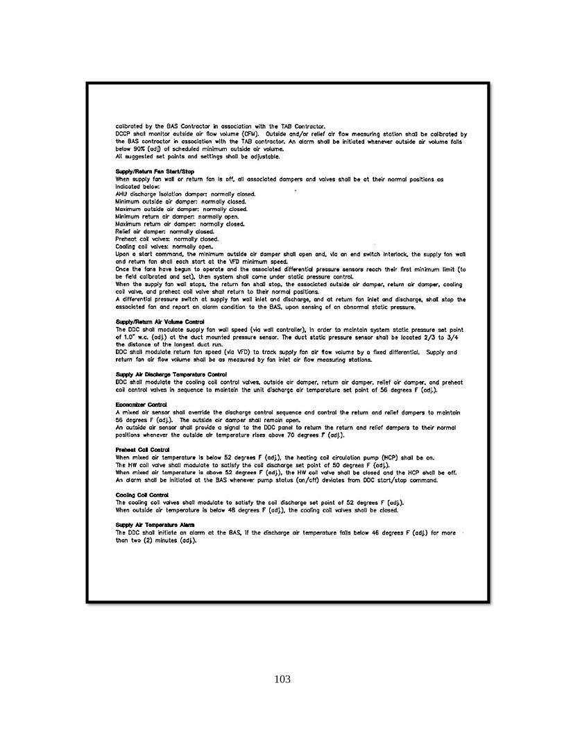
103
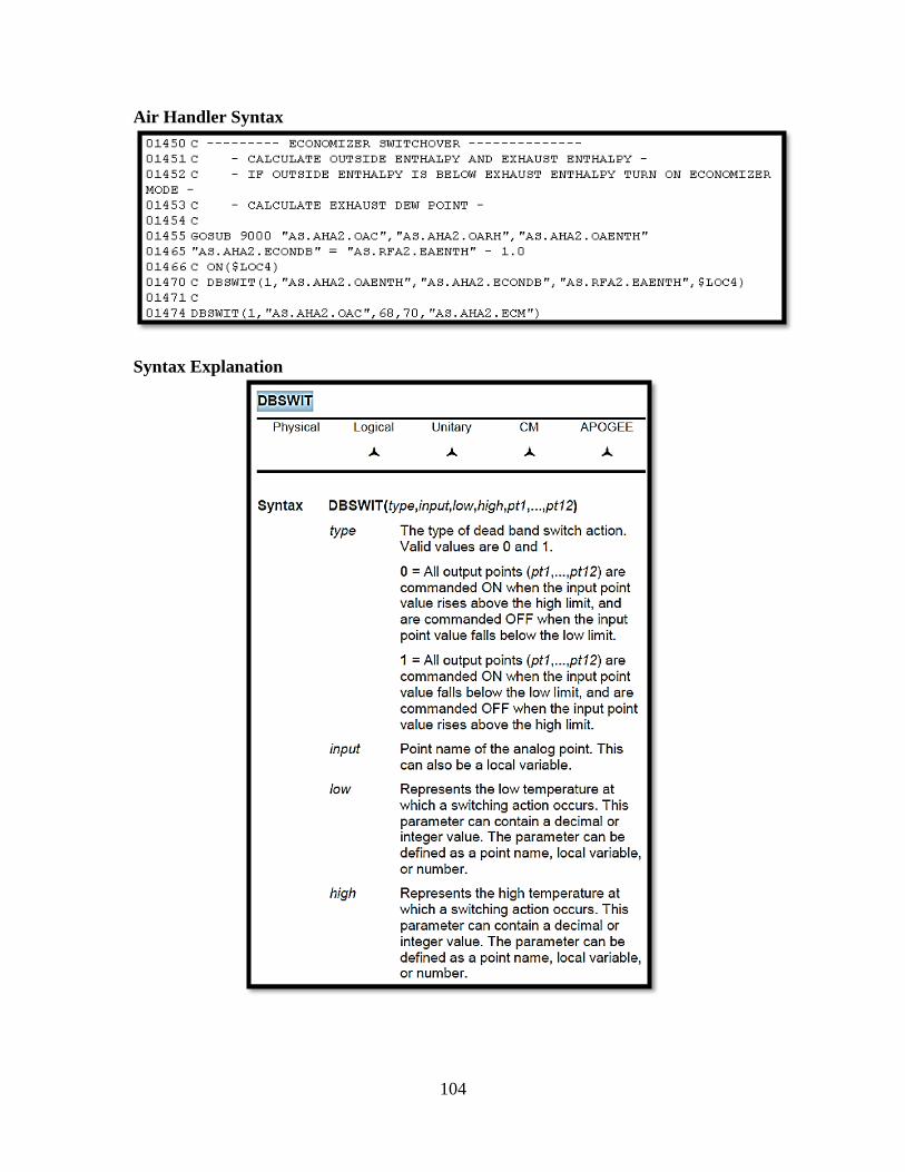
104
Air Handler Syntax
Syntax Explanation