Utility Maximization and Choice - University at Albany, SUNYby872279/micro/Slides/utility2.… · · 2014-09-02Utility Maximization and Choice ... • Nothing in the model prevents

PowerPoint Slides prepared by: Andreea CHIRITESCU

Eastern Illinois University

Utility Maximization

and Choice

© 2012 Cengage Learning. All Rights Reserved. May not be copied, scanned, or duplicated, in whole or in part, except for use as permitted in a license distributed with a certain product or service or otherwise on a password-protected website for classroom use.

1

Utility Maximization and Choice

• Complaints about the Economic Approach– Do individuals make the “lightning

calculations” required for utility maximization?• The utility-maximization model predicts many

aspects of behavior• Economists assume that people behave as if

they made such calculations

2© 2012 Cengage Learning. All Rights Reserved. May not be copied, scanned, or duplicated, in whole or in part, except for use as permitted in a license distributed with a certain product or service or otherwise on a password-protected website for classroom use.

Utility Maximization and Choice

• Complaints about the Economic Approach– The economic model of choice is

extremely selfish• Nothing in the model prevents individuals

from getting satisfaction from “doing good”


An Initial Survey

• Optimization principle, Utility maximization– To maximize utility, given a fixed amount

of income to spend– An individual will buy those quantities of

goods • That exhaust his or her total income • And for which the MRS is equal to the rate at

which the goods can be traded one for the other in the marketplace

– MRS (of x for y) = the ratio of the price of x to the price of y (px/py)


The Two-Good Case

• Assumptions – Budget: I dollars to allocate between good

x and good y– px - price of good x – py - price of good y

• Budget constraint: pxx + pyy ≤ I – Slope = -px/py

– If all of I is spent on good x, buy I/px units of good x


4.1The Individual’s Budget Constraint for Two Goods

Those combinations of x and y that the individual can afford are shown in the shaded triangle. If, as we usually assume, the individual prefers more rather than less of every good, the outer boundary of this triangle is the relevant constraint where all the available funds are spent either on x or on y. The slope of this straight-line boundary is given by –px/py.


I=pxx+pyy

ypI

xpI

Quantity of x

Quantity of y

The Two-Good Case

• First-order conditions for a maximum– Point of tangency between the budget

constraint and the indifference curve:


U=constant

slope of budget constraint=slope of indifference curve

=- (of for )x

y

p dyMRS x y

p dx=

4.2A Graphical Demonstration of Utility Maximization

Point C represents the highest utility level that can be reached by the individual, given the budget constraint. Therefore, the combination x*,y* is the rational way for the individual to allocate purchasing power. Only for this combination of goods will two conditions hold: All available funds will be spent, and the individual’s psychic rate of trade-off (MRS) will be equal to the rate at which the goods can be traded in the market ( px/py).


I=pxx+pyy

Quantity of x

Quantity of y

U1

U3

D

U2A

B

Cy*

x*

The Two-Good Case

• The tangency rule – Is necessary but not sufficient unless we

assume that MRS is diminishing• If MRS is diminishing, then indifference

curves are strictly convex• If MRS is not diminishing, we must check

second-order conditions to ensure that we are at a maximum


4.3Example of an Indifference Curve Map for Which the Tangency Condition Does Not Ensure a Maximum

If indifference curves do not obey the assumption of a diminishing MRS, not all points of tangency (points for which MRS = px/py) may truly be points of maximum utility. In this example, tangency point C is inferior to many other points that can also be purchased with the available funds. In order that the necessary conditions for a maximum (i.e., the tangency conditions) also be sufficient, one usually assumes that the MRS is diminishing; that is, the utility function is strictly quasi-concave.


Quantity of x

Quantity of y

U1

U3

U2

CA

B

The Two-Good Case

• Corner solutions– Individuals may maximize utility by

choosing to consume only one of the goods

– At the optimal point the budget constraint is flatter than the indifference curve• The rate at which x can be traded for y in the

market is lower than the MRS


4.4Corner Solution for Utility Maximization

With the preferences represented by this set of indifference curves, utility maximization occurs at E, where 0 amounts of good y are consumed. The first-order conditions for a maximum must be modified somewhat to accommodate this possibility.


Quantity of x

Quantity of yU2 U3

U1

x*

The n-Good Case

• The individual’s objective is to maximize

utility = U(x1,x2,…,xn)

subject to the budget constraint

I = p1x1 + p2x2 +…+ pnxn

• Set up the Lagrangian:

ℒℒℒℒ = U(x1,x2,…,xn) + λ(I - p1x1 - p2x2 -…- pnxn)


The n-Good Case

• First-order conditions for an interior

maximum

∂ℒℒℒℒ/∂x1 = ∂U/∂x1 - λp1 = 0

∂ℒℒℒℒ /∂x2 = ∂U/∂x2 - λp2 = 0

…

∂ℒℒℒℒ /∂xn = ∂U/∂xn - λpn = 0

∂ℒℒℒℒ /∂λ = I - p1x1 - p2x2 - … - pnxn = 0


The n-Good Case

• Implications of first-order conditions

– For any two goods, xi and yj:


/ ( for )

/i i

i jj j

U x pMRS x x

U x p

∂ ∂ = =∂ ∂

The n-Good Case

• Interpreting the Lagrange multiplier

– λ is the marginal utility of an extra dollar of consumption expenditure• The marginal utility of income


1 2

1 2

// /... n

n

U xU x U x

p p pλ ∂ ∂∂ ∂ ∂ ∂= = = =

The n-Good Case

• At the margin, the price of a good– Represents the consumer’s evaluation of

the utility of the last unit consumed– How much the consumer is willing to pay

for the last unit


/, for every i

i

U xp i

λ∂ ∂=

The n-Good Case

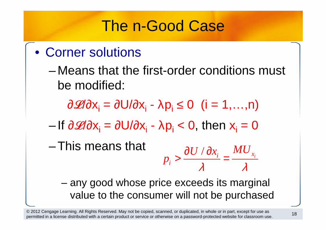
• Corner solutions– Means that the first-order conditions must

be modified:

∂ℒℒℒℒ/∂xi = ∂U/∂xi - λpi ≤ 0 (i = 1,…,n)

– If ∂ℒℒℒℒ/∂xi = ∂U/∂xi - λpi < 0, then xi = 0

– This means that


/ixi

i

MUU xp

λ λ∂ ∂> =

– any good whose price exceeds its marginal value to the consumer will not be purchased

4.1 Cobb–Douglas Demand Functions

• Cobb-Douglas utility function:U(x,y) = xαyβ

• Setting up the Lagrangian:

ℒℒℒℒ = xαyβ + λ(I - pxx - pyy)

• First-order conditions:

∂ℒℒℒℒ/∂x = αxα-1yβ - λpx = 0

∂ℒℒℒℒ/∂y = βxαyβ-1 - λpy = 0

∂ℒℒℒℒ/∂λ = I - pxx - pyy = 0



• First-order conditions imply: αy/βx = px/py

• Since α + β = 1: pyy = (β/α)pxx = [(1- α)/α]pxx

• Substituting into the budget constraint:

I = pxx + [(1- α)/α]pxx = (1/α)pxx

• Solving: x*=αI/px and y*=βI/py

• The individual will allocate α percent of his

income to good x and β percent of his income to

good y



• Cobb-Douglas utility function• Is limited in its ability to explain actual

consumption behavior• The share of income devoted to a good often

changes in response to changing economic conditions

• A more general functional form might be more useful


4.2 CES Demand

• Assume that δ = 0.5

U(x,y) = x0.5 + y0.5

• Setting up the Lagrangian:

ℒℒℒℒ = x0.5 + y0.5 + λ(I - pxx - pyy)

• First-order conditions for a maximum:

∂ℒℒℒℒ/∂x = 0.5x -0.5 - λpx = 0

∂ℒℒℒℒ/∂y = 0.5y -0.5 - λpy = 0

∂ℒℒℒℒ/∂λ = I - pxx - pyy = 0


4.2 CES Demand

• This means that: (y/x)0.5 = px/py

• Substituting into the budget constraint, we can solve for the demand functions


*[1 ( / )]x x y

xp p p

=+I

*[1 ( / )]y y x

yp p p

=+I

• The share of income spent on either x or y is not a constant• Depends on the ratio of the two prices

• The higher is the relative price of x, the smaller will be the share of income spent on x

4.2 CES Demand

• If δ = -1,

U(x,y) = -x -1 - y -1

• First-order conditions imply that

y/x = (px/py)0.5

• The demand functions are


0.5*

1 yx

x

xp

pp

= +

I0.5

*

1 xy

y

yp

pp

= +

I

4.2 CES Demand

• If δ = -∞, U(x,y) = Min(x,4y)• The person will choose only combinations for

which x = 4y

• This means that

I = pxx + pyy = pxx + py(x/4)

I = (px + 0.25py)x

• The demand functions are


*0.25x y

xp p

=+I

*4 x y

yp p

=+I

Indirect Utility Function

• It is often possible to manipulate first-order conditions to solve for optimal values of x1,x2,…,xn

– These optimal values will bex*1 = x1(p1,p2,…,pn,I)

x*2 = x2(p1,p2,…,pn,I)

…

x*n = xn(p1,p2,…,pn,I)


Indirect Utility Function

• We can use the optimal values of the x’s to find the indirect utility function

maximum utility = U[x*1(p1,p2,…,pn,I), x*2(p1,p2,…,pn,I),…,x*n(p1,p2,…,pn,I)] =

= V(p1,p2,…,pn,I)

• The optimal level of utility will depend indirectly on prices and income


The Lump Sum Principle

• Taxes on an individual’s general purchasing power – Are superior to taxes on a specific good

• An income tax allows the individual to decide freely how to allocate remaining income

• A tax on a specific good will reduce an individual’s purchasing power and distort his choices


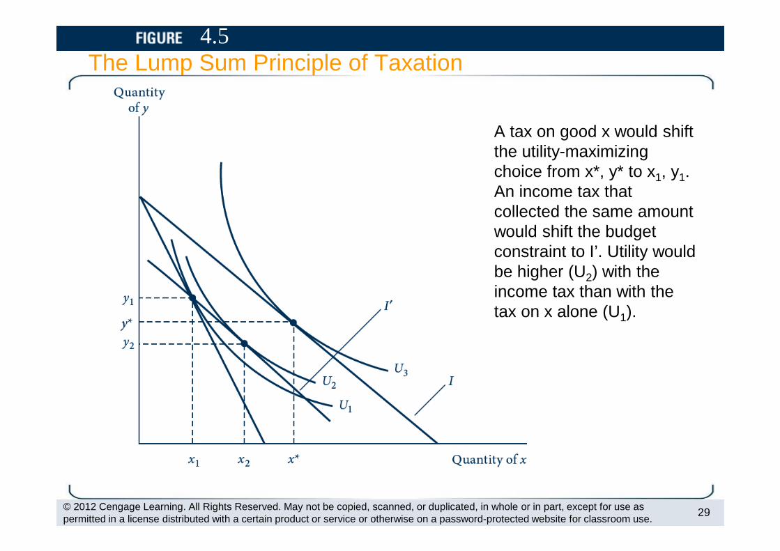
4.5The Lump Sum Principle of Taxation


A tax on good x would shift the utility-maximizing choice from x*, y* to x1, y1. An income tax that collected the same amount would shift the budget constraint to I’. Utility would be higher (U2) with the income tax than with the tax on x alone (U1).

4.3 Indirect Utility and the Lump Sum Principle

• Cobb-Douglas utility function• With α = β = 0.5, • We know that

x*=I/2px and y*=I/2py

• The indirect utility function


0 5 0 50.5 0.5

( , , ) 2

. .x y

x y

V p p (x*) (y*)p p

= = II


• Fixed proportionsx*=I/[px + 0.25py] and y*=I/[4px+py]

• The indirect utility function


( , , ) min( *,4 *)

* 0.25

4 *4

x y

x y

x y

V p p x y

xp p

yp p

= =

= = =+

= =+

I

I

4


• The lump sum principle• Cobb-Douglas

• If a tax of $1 was imposed on good x• The individual will purchase x* = 2• Indirect utility will fall from 2 to 1.41

• An equal-revenue tax will reduce income to $6• Indirect utility will fall from 2 to 1.5



• The lump sum principle• Fixed-proportions

• If a tax of $1 was imposed on good x• Indirect utility will fall from 4 to 8/3

• An equal-revenue tax will reduce income to $16/3• Indirect utility will fall from 4 to 8/3

• Since preferences are rigid, the tax on x does not distort choices


Expenditure Minimization

• Dual minimization problem for utility maximization– Allocate income to achieve a given level of

utility with the minimal expenditure• The goal and the constraint have been

reversed


4.6The Dual Expenditure-Minimization Problem

The dual of the utility-maximization problem is to attain a given utility level (U2) with minimal expenditures. An expenditure level of E1 does not permit U2 to be reached, whereas E3 provides more spending power than is strictly necessary. With expenditure E2, this person can just reach U2 by consuming x and y.


E2

Quantity of x

Quantity of y

U2

E1

E3

B

C

Ay*

x*


• The individual’s problem is to choose x1,x2,…,xn to minimize

total expenditures = E = p1x1 + p2x2 +…+ pnxn

subject to the constraint

utility = Ū = U(x1,x2,…,xn)

– The optimal amounts of x1,x2,…,xn will depend on the prices of the goods and the required utility level



• Expenditure function– The individual’s expenditure function – Shows the minimal expenditures– Necessary to achieve a given utility level – For a particular set of prices

• minimal expenditures = E(p1,p2,…,pn,U)



• The expenditure function and the indirect utility function – Are inversely related– Both depend on market prices – But involve different constraints


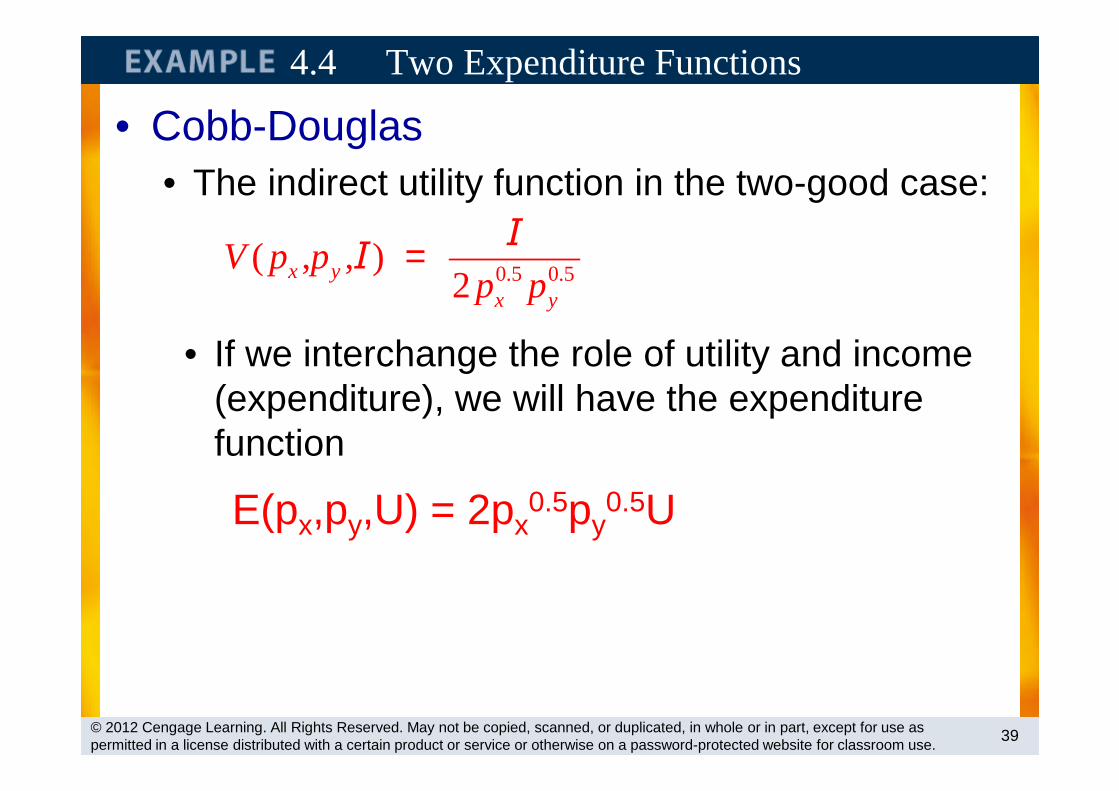
4.4 Two Expenditure Functions

• Cobb-Douglas • The indirect utility function in the two-good case:


0.5 0.5( , , )

2x yx y

V p pp p

= II

• If we interchange the role of utility and income (expenditure), we will have the expenditure function

E(px,py,U) = 2px0.5py

0.5U

4.4 Two Expenditure Functions

• Fixed-proportions case• The indirect utility function:


• If we interchange the role of utility and income (expenditure), we will have the expenditure function

E(px,py,U) = (px + 0.25py)U

( , , ) 0.25x y

x y

V p pp p

=+I

I

Properties of Expenditure Functions

• Homogeneity– A doubling of all prices will precisely

double the value of required expenditures• Homogeneous of degree one

• Nondecreasing in prices– ∂E/∂pi ≥ 0 for every good, i

• Concave in prices – Functions that always lie below tangents

to them


4.7Expenditure Functions Are Concave in Prices

At p1 this person spends E(p1* , . . .). If he or she continues to buy the same set of goods as p1 changes, then expenditures would be given by Epseudo. Because his or her consumption patterns will likely change as p1 changes, actual expenditures will be less than this.


E(p1,…)

Epseudo

p1

E(p1,…)

E(p*1,…)

p*1

Budget Shares

• Engel’s law – Fraction of income spent on food

decreases as income increases

• Budget shares, si=pixi / I• Recent budget share data

– Engel’s law is clearly visible

• Cobb–Douglas utility function – Is not useful for detailed empirical studies

of household behavior


E4.1Budget shares of U.S. households, 2008


Linear expenditure system

• Generalization of the Cobb–Douglas function– Incorporates the idea that certain minimal

amounts of each good must be bought by an individual (x0, y0)

U(x,y)=(x-x0)α(y-y0)β

• For x ≥ x0 and y ≥ y0, • Where α+β=1


Linear expenditure system

• Supernumerary income (I*)– Amount of purchasing power remaining

after purchasing the minimum bundleI*=I-pxx0-pyy0

• The demand functions are:x = (pxx0+αI*)/px and y = (pyy0+βI*)/py

– The share equations:sx= α+(βpxx0-αpyy0)/I sx= β+(αpyy0 -βpxx0)/I

• Not homothetic46© 2012 Cengage Learning. All Rights Reserved. May not be copied, scanned, or duplicated, in whole or in part, except for use as

permitted in a license distributed with a certain product or service or otherwise on a password-protected website for classroom use.

CES utility

• CES utility function


( , ) , for 1, 0x y

U x yδ δ

δ δδ δ

= + ≤ ≠

• Budget shares:sx=1/[1+(py/px)K] and sy=1/[1+(px/py)K]

• Where K = δ/(δ-1)

• Homothetic

The almost ideal demand system

• Expenditure functions– Logarithmic differentiation


ln ( , , ) 1

ln ( , , ) lnx y x x

xx x y x x

E p p V p xpEs

p E p p V p p E

∂ ∂∂= ⋅ ⋅ = =∂ ∂ ∂


• Almost ideal demand system– Expenditure function


1 2

0 1 2

21 2

23 0

ln ( , , ) ln ln

0.5 (ln ) ln ln

0.5 (ln )

x y x y

x x y

c cy x y

E p p V a a p a p

b p b p p

b p Vc p p

= + + +

+ + +

+ +

• Almost ideal demand system– Expenditure function



1 2

1 2

1 1 2 1 0

2 2 3 2 0

1 1

20 1 2 1

2 1

2 2

2

2 3

ln ln

ln ln

1

is an index of prices

ln ln l

ln

n 0.5 (ln )

l

ln ( / )

ln ln

n l

( / )

n 0.5

c cx x y x y

c c

x x y

y x

y x y x y

x y

x y

x y

y

x

s a b p b p c E p

s

s a b p b p c Vc p p

s a b p b p c Vc p p

s s

p

p a

a b p

a p a p

b

b p

b p

p

p

p

b

c E

= + + +

= + + +

= +

+ =

= + + + +

+

+ +

+

= + + +

23(ln )yp

Documents

Utility Maximization and Choice - University at Albany, SUNYby872279/micro/Slides/utility2.… · · 2014-09-02Utility Maximization and Choice ... • Nothing in the model prevents