Utility Accrual Real-Time Scheduling for

Multiprocessor Embedded Systems

Hyeonjoong Cho a Binoy Ravindran b E. Douglas Jensen c

aDept. of Computer and Information Science, Korea University, South KoreabECE Dept., Virginia Tech., Blacksburg, VA 24061, USA

cThe MITRE Corporation Bedford, MA 01730, USA

Abstract

We present the first Utility Accrual (or UA) real-time scheduling algorithm for mul-tiprocessors, called global Multiprocessor Utility Accrual scheduling algorithm (orgMUA). The algorithm considers an application model where real-time activitiesare subject to time/utility function time constraints, variable execution time de-mands, and resource overloads where the total activity utilization demand exceedsthe total capacity of all processors. We consider the scheduling objective of (1)probabilistically satisfying lower bounds on each activity’s maximum utility, and(2) maximizing the system-wide, total accrued utility. We establish several proper-ties of gMUA including optimal total utility (for a special case), conditions underwhich individual activity utility lower bounds are satisfied, a lower bound on system-wide total accrued utility, and bounded sensitivity for assurances to variations inexecution time demand estimates. Finally, our simulation experiments validate ouranalytical results and confirm the algorithm’s effectiveness.

Key words: Time utility function, utility accrual, multiprocessor systems,statistical assurance, real-time, scheduling

Email addresses: raycho@korea.ac.kr (Hyeonjoong Cho), binoy@vt.edu(Binoy Ravindran), jensen@mitre.org (E. Douglas Jensen).

Preprint submitted to Elsevier 8 May 2009

1 Introduction

1.1 Utility Accrual Real-Time Scheduling

There are embedded real-time systems in many domains, such as robotic sys-tems in the space domain (e.g., NASA/JPL’s Mars Rover [1]) and controlsystems in the defense domain (e.g., airborne trackers [2]), which are funda-mentally distinguished by the fact that they operate in environments with dy-namically uncertain properties. These uncertainties include transient and sus-tained resource overloads due to context-dependent activity execution timesand arbitrary activity arrival patterns. Nevertheless, such systems desire thestrongest possible assurances on activity timeliness behavior. Another impor-tant distinguishing feature of almost all of these systems is their relatively longtask execution time magnitudes—e.g., in the order of milliseconds to minutes.

When resource overloads occur, meeting deadlines of all activities is impossibleas the demand exceeds the supply. The urgency of an activity is typically or-thogonal to its relative importance—e.g., the most urgent activity can be theleast important, and vice versa; the most urgent can be the most important,and vice versa. Hence when overloads occur, completing the most importantactivities irrespective of activity urgency is often desirable. Thus, a clear dis-tinction has to be made between urgency and importance during overloads.During under-loads, such a distinction need not be made, because deadline-based scheduling algorithms such as EDF are optimal (on one processor) [3].

Deadlines by themselves cannot express both urgency and importance. Thus,we consider the abstraction of time/utility functions (or TUFs) [4] that expressthe utility of completing an application activity as a function of that activity’scompletion time. We specify a deadline as a binary-valued, downward “step”shaped TUF; Figure 1(a) shows examples. Note that a TUF decouples impor-tance and urgency—i.e., urgency is measured as a deadline on the X-axis, andimportance is denoted by utility on the Y-axis.

-Time

6Utility

0(a)

-Time

6Utility

0

bbb

(b)

-Time

6UtilitySSS

0

HH

(c)

Fig. 1. Example TUF Time Constraints: (a) Step TUFs; (b) AWACS TUF [2]; and(c) Coastal Air defense TUFs [5]

Many embedded real-time systems also have activities that are subject to non-deadline time constraints, such as those where the utility attained for activitycompletion varies (e.g., decreases, increases) with completion time. This is incontrast to deadlines, where a positive utility is attained for completing the ac-

2

tivity anytime before the deadline, after which zero, or infinitely negative util-ity is attained. Figures 1(a)-1(c) show examples of such time constraints fromtwo real applications (see [2] and references therein for application details).For example, in [2], Clark at. al. discuss an AWACS tracker application whichcollects radar sensor reports, identifies airborne objects (or “track objects”)in them, and associates those objects to track states that are maintained ina track database. Here, each job of a track association task has a TUF timeconstraint, and all jobs of the same task have the same time constraint. Thetracker is routinely overloaded, so the collective timeliness optimality criterionis to meet as many job deadlines (or termination times) as possible, and tomaximize the total utility obtained from the completion of as many jobs aspossible. Another example timeliness requirement is found in a NASA/JPLMars Science Lab Rover application—scheduling of processor cycles for theMission Data System (MDS) [1]. Additional key features of this applicationinclude transient and permanent processor cycle overloads, and activity timescales (e.g., frequency of constructing MDS schedules) that are of the order ofminutes.

When activity time constraints are specified using TUFs, which subsume dead-lines, the scheduling criteria are based on accrued utility, such as maximizingsum of the activities’ attained utilities. We call such criteria, utility accrual(or UA) criteria, and scheduling algorithms that optimize them UA schedulingalgorithms.

On single processors, UA algorithms that maximize accrued utility for down-ward step TUFs (see algorithms in [6]) default to EDF during under-loads,since EDF satisfies all deadlines during under-loads. Consequently, they obtainthe maximum possible accrued utility during under-loads. During overloads,they favor more important activities (since more utility can be attained fromthem), irrespective of urgency. Thus, deadline scheduling’s optimal timelinessbehavior is a special case of UA scheduling.

1.2 Real-time Scheduling on Multiprocessors

Multiprocessor architectures—e.g., Symmetric Multi-Processors (SMPs), Sin-gle Chip Heterogeneous Multiprocessors (SCHMs)—are recently becomingmore attractive for embedded systems because they are significantly decreas-ing in price. This makes them very desirable for embedded system applicationswith high computational workloads, where additional, cost-effective process-ing capacity is often needed. Responding to this trend, (real-time operat-ing system) RTOS vendors are increasingly providing multiprocessor platformsupport—e.g., QNX Neutrino is now available for a variety of SMP chips [7].But this exposes the critical need for real-time scheduling for multiprocessors—

3

a comparatively undeveloped area of real-time scheduling which has recentlyreceived significant research attention, but is not yet well supported by theRTOS products. Consequently, the impact of cost-effective multiprocessorplatforms for embedded systems remains nascent.

One highly developed class of multiprocessor scheduling algorithms is staticscheduling of a program represented by a directed task graph on a multiproces-sor system to minimize the program completion time [8]. In contrast to that,the class of multiprocessor scheduling algorithms our work is in seeks to satisfytasks’ completion time constraints (such as deadlines) by performing dynamic(i.e., run-time) task assignment to processors and dynamic scheduling of thetasks on each processor.

One unique aspect of multiprocessor scheduling is the degree of run-time mi-gration that is allowed for job instances of a task across processors (at schedul-ing events). Example migration models include: (1) full migration, wherejobs are allowed to arbitrarily migrate across processors during their execu-tion. This usually implies a global scheduling strategy, where a single sharedscheduling queue is maintained for all processors and a system-wide schedulingdecision is made by a single (global) scheduling algorithm; (2) no migration,where tasks are statically (off-line) partitioned and allocated to processors. Atrun-time, job instances of tasks are scheduled on their respective processorsby processors’ local scheduling algorithm, like single processor scheduling; and(3) restricted migration, where some form of migration is allowed—e.g., at jobboundaries.

Carpentar et al. [9] have catalogued multiprocessor real-time scheduling al-gorithms considering the degree of job migration. The Pfair class of algo-rithms [10] that allow full migration have been shown to achieve a schedu-lable utilization bound (below which all tasks meet their deadlines) thatequals the total capacity of all processors—thus, they are theoretically optimal.However, Pfair algorithms incur significant overhead due to their quantum-based scheduling approach [11]. Thus, scheduling algorithms other than Pfair(e.g., global EDF) have also been studied though their schedulable utilizationbounds are lower.

Global EDF scheduling on multiprocessors is subject to the “Dhall effect” [12],where a task set with total utilization demand arbitrarily close to one can-not be scheduled so as to satisfy all deadlines. To overcome this, researchershave studied global EDF’s behavior under restricted individual task utiliza-tions. For example, on M processors, Srinivasan and Baruah show that whenthe maximum individual task utilization, umax, is bounded by M/ (2M − 1),EDF’s utilization bound is M2/ (2M − 1) [13]. In [14], Goossens et. al showthat EDF’s utilization bound is M − (M − 1) umax. This work was later ex-tended by Baker for the more general case of deadlines less than or equal to

4

periods in [15]. In [16], Bertogna et al. show that Baker’s utilization bounddoes not dominate the bound of Goossens et. al, and vice versa.

While most of these past works focus on the hard real-time objective of al-ways meeting all deadlines, recently there have been efforts that consider thesoft real-time objective of bounding the tardiness of tasks. In [17], Srinivasanand Anderson derive a tardiness bound for a suboptimal Pfair scheduling algo-rithm. In [25], for a restricted migration model where migration is allowed onlyat job boundaries, Andersen et. al present an EDF-based partitioning schemeand scheduling algorithm that ensures bounded tardiness. In [11], Devi andAnderson derive the tardiness bounds for global EDF when the total utiliza-tion demand of tasks may equal the number of available processors.

1.3 Contributions

In this paper, we consider the problem of global UA scheduling on an SMPsystem with M number of identical processors in environments with dynam-ically uncertain properties. By dynamic uncertainty, we mean operating inenvironments where arrival and execution behaviors of tasks are subject torun-time uncertainties, causing resource overloads. Nonetheless, such systemsdesire the strongest possible assurances on task timing behaviors—both thatof individual activities behavior and that of collective, system-wide behavior.Statistical assurances are appropriate for these systems.

Multiprocessor scheduling should determine which processor each task shouldbe assigned to for execution (the allocation problem) and in which ordertasks should start execution at each processor (the scheduling problem). Ourscheduling algorithm does both.

Real-time scheduling for multiprocessors is categorized into: global scheduling,where all jobs are scheduled together based on a single queue for all proces-sors; partitioned scheduling, where tasks are assigned to processors, and eachprocessor is scheduled separately. We consider global multiprocessor schedul-ing (that allows full migration as opposed to partitioned scheduling) becauseof its improved schedulability and flexibility [18]. Further, in many embeddedarchitectures (e.g., those with no cache), its migration overhead has a lowerimpact on performance [16]. Moreover, applications of interest to us [1,2] areoften subject to resource overloads, during when the total application utiliza-tion demand exceeds the total processing capacity of all processors. Whenthat happens, we hypothesize that global scheduling has greater schedulingflexibility, resulting in greater accrued activity utility, than does partitionedscheduling.

We consider repeatedly occurring application activities (e.g., tasks) that are

5

subject to TUF time constraints, variable execution times, and overloads. Toaccount for uncertainties in activity execution behaviors, we employ a stochas-tic model for activity demand and execution. Activities repeatedly arrive witha known minimum inter-arrival time. For such a model, our objective is to:(1) provide statistical assurances on individual activity timeliness behaviorincluding probabilistically-satisfied lower bounds on each activity’s maximumutility; (2) provide assurances on system-level timeliness behavior includingan assured lower bound on the sum of the activities’ attained utilities; and(3) maximize the sum of activities’ attained utilities.

This problem has not been studied in the past and is NP-hard. We presenta polynomial-time, heuristic algorithm for the problem called the global Mul-tiprocessor Utility Accrual (gMUA) scheduling algorithm. We establish sev-eral properties of gMUA including optimal total utility for the special caseof downward step TUFs and application utilization demand not exceedingglobal EDF’s utilization bound—conditions under which individual activityutility lower bounds are satisfied, and a lower bound is established on system-wide total accrued utility. We also show that the algorithm’s assurances havebounded sensitivity to variations in execution time demand estimates, in thesense that the assurances hold as long as the variations satisfy a sufficient con-dition that we present. Further, we show that the algorithm is robust againsta variant of the Dhall effect.

Thus, the contribution of this paper is the gMUA algorithm. We are not awareof any other efforts that solve the problem solved by gMUA.

The rest of the paper is organized as follows: Section 2 describes our modelsand scheduling objective. In Section 3, we discuss the rationale behind gMUAand present the algorithm. We describe the algorithm’s properties in Section 4.We report our simulation-based experimental studies in Section 5. The paperconcludes in Section 6.

2 Models and Objective

2.1 Activity Model

We consider the application to consist of a set of tasks, denoted T={T1, T2, ...,Tn}. Each task Ti has a number of instances, called jobs, and these jobs maybe released either periodically or sporadically with a known minimal inter-arrival time. The jth job of task Ti is denoted as Ji,j. The period or minimalinter-arrival time of a task Ti is denoted as pi.

6

We initially assume that all tasks are independent—i.e., they do not share anyresource or have any precedences.

The basic scheduling entity that we consider is the job abstraction. Thus, weuse J to denote a job without being task specific, as seen by the scheduler atany scheduling event.

A job’s time constraint is specified using a TUF. Jobs of the same task havethe same TUF. We use Ui() to denote the TUF of task Ti. Thus, completionof the job Ji,j at time t will yield an utility of Ui(t).

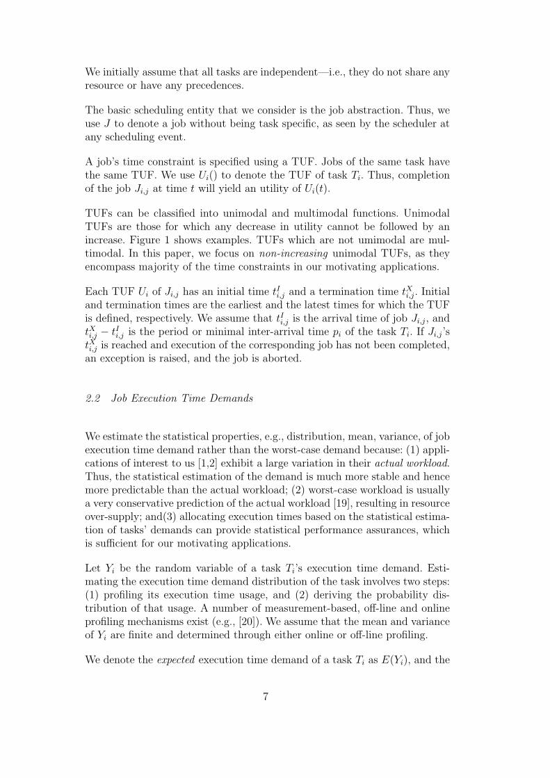
TUFs can be classified into unimodal and multimodal functions. UnimodalTUFs are those for which any decrease in utility cannot be followed by anincrease. Figure 1 shows examples. TUFs which are not umimodal are mul-timodal. In this paper, we focus on non-increasing unimodal TUFs, as theyencompass majority of the time constraints in our motivating applications.

Each TUF Ui of Ji,j has an initial time tIi,j and a termination time tXi,j. Initialand termination times are the earliest and the latest times for which the TUFis defined, respectively. We assume that tIi,j is the arrival time of job Ji,j, andtXi,j − tIi,j is the period or minimal inter-arrival time pi of the task Ti. If Ji,j’stXi,j is reached and execution of the corresponding job has not been completed,an exception is raised, and the job is aborted.

2.2 Job Execution Time Demands

We estimate the statistical properties, e.g., distribution, mean, variance, of jobexecution time demand rather than the worst-case demand because: (1) appli-cations of interest to us [1,2] exhibit a large variation in their actual workload.Thus, the statistical estimation of the demand is much more stable and hencemore predictable than the actual workload; (2) worst-case workload is usuallya very conservative prediction of the actual workload [19], resulting in resourceover-supply; and(3) allocating execution times based on the statistical estima-tion of tasks’ demands can provide statistical performance assurances, whichis sufficient for our motivating applications.

Let Yi be the random variable of a task Ti’s execution time demand. Esti-mating the execution time demand distribution of the task involves two steps:(1) profiling its execution time usage, and (2) deriving the probability dis-tribution of that usage. A number of measurement-based, off-line and onlineprofiling mechanisms exist (e.g., [20]). We assume that the mean and varianceof Yi are finite and determined through either online or off-line profiling.

We denote the expected execution time demand of a task Ti as E(Yi), and the

7

variance on the demand as V ar(Yi).

2.3 Statistical Timeliness Requirement

We consider a task-level statistical timeliness requirement—each task mustattain some percentage of its maximum possible utility with a certain prob-ability. For a task Ti, this requirement is specified as {νi, ρi}, which impliesthat Ti must attain at least νi percentage of its maximum possible utility withthe probability ρi. This is also the requirement for each job of Ti. Thus, forexample, if {νi, ρi} = {0.7, 0.93}, then Ti must attain at least 70% of its max-imum possible utility with a probability no less than 93%. For step TUFs, νcan only take the value 0 or 1. Note that the objective of always satisfying alltask deadlines is the special case of {νi, ρi} = {1.0, 1.0}.

This statistical timeliness requirement on the utility of a task implies a corre-sponding requirement on the range of its job sojourn times. 1 Since we focus onnon-increasing unimodal TUFs, upper-bounding job sojourn times will lower-bound job and task utilities.

2.4 Scheduling Objective

We consider a two-fold scheduling criterion: (1) assure that each task Ti at-tains the specified percentage νi of its maximum possible utility with at leastthe specified probability ρi; and (2) maximize the system-level total accruedutility. We also desire to obtain a lower bound on the system-level total ac-crued utility. When it is not possible to satisfy ρi for each task (e.g., due tooverloads), our objective is to maximize the system-level total accrued utility.

This problem is NP-hard because it subsumes the NP-hard problem ofscheduling dependent tasks with step TUFs on one processor [21].

1 A job’s sojourn time is defined as the time interval from the job’s release to itscompletion.

8

3 The gMUA Algorithm

3.1 Bounding Accrued Utility

Let si,j be the sojourn time of the jth job of task Ti. Task Ti’s statisticaltimeliness requirement can be represented as Pr(Ui(si,j) ≥ νi × Umax

i ) ≥ ρi,where Umax

i is the maximum value of Ui(). Since TUFs are assumed to be non-increasing, it is sufficient to have Pr(si,j ≤ Di) ≥ ρi, where Di is the upperbound on the sojourn time of task Ti. We call Di the “critical time” hereafter,and it is calculated as Di = U−1

i (νi×Umaxi ), where U−1

i (x) denotes the inversefunction of TUF Ui(). Thus, Ti is (probabilistically) assured to attain at leastthe utility percentage νi = Ui(Di)/U

maxi , with the probability ρi.

3.2 Bounding Utility Accrual Probability

Since task execution time demands are stochastically specified (through meansand variances), we need to determine the actual execution time that must beallocated to each task, such that the desired utility attained probability ρi issatisfied. Further, this execution time allocation must account for the uncer-tainty in the execution time demand specification (i.e., the variance factor).

Given the mean and the variance of a task Ti’s execution time demand Yi, bya one-tailed version of the Chebyshev’s inequality, when y ≥ E(Yi), we have:

Pr[Yi < y] ≥ (y − E(Yi))2

V ar(Yi) + (y − E(Yi))2(1)

From a probabilistic point of view, Equation 1 is the direct result of thecumulative distribution function of task Ti’s execution time demands—i.e.,Fi(y) = Pr[Yi ≤ y]. Recall that each job of task Ti must attain νi percentage ofits maximum possible utility with a probability ρi. To satisfy this requirement,

we let ρ′i = Pr[Yi < Ci] = (Ci−E(Yi))2

V ar(Yi)+(Ci−E(Yi))2 ≥ ρi and obtain the minimum

required execution time Ci = E(Yi) +√

ρ′i×V ar(Yi)1−ρ′i

.

Thus, the gMUA algorithm allocates Ci execution time units to each job Ji,jof task Ti, so that the probability that job Ji,j requires no more than theallocated Ci execution time units is at least ρi—i.e., Pr[Yi < Ci] ≥ ρ′i ≥ ρi.

We set ρ′i = (max {ρi}) 1n , ∀i to satisfy requirements given by ρi. Supposing

that each task is allocated Ci time within its pi, the actual demand of eachtask often varies. Some jobs of the task may complete their execution before

9

using up their allocated time, and the others may not. gMUA probabilisticallyschedules the jobs of a task Ti to provide assurance probability ρ′i (≥ ρi) aslong as they are satisfying a certain feasibility test.

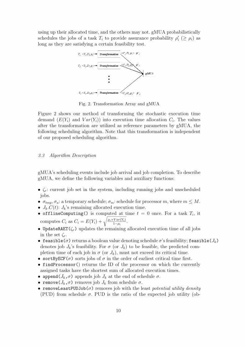
Fig. 2. Transformation Array and gMUA

Figure 2 shows our method of transforming the stochastic execution timedemand (E(Yi) and V ar(Yi)) into execution time allocation Ci. The valuesafter the transformation are utilized as reference parameters by gMUA, thefollowing scheduling algorithm. Note that this transformation is independentof our proposed scheduling algorithm.

3.3 Algorithm Description

gMUA’s scheduling events include job arrival and job completion. To describegMUA, we define the following variables and auxiliary functions:

• ζr: current job set in the system, including running jobs and unscheduledjobs.• σtmp, σa: a temporary schedule; σm: schedule for processor m, where m ≤M .• Jk.C(t): Jk’s remaining allocated execution time.• offlineComputing() is computed at time t = 0 once. For a task Ti, it

computes Ci as Ci = E(Yi) +√

ρi×V ar(Yi)1−ρi .

• UpdateRAET(ζr) updates the remaining allocated execution time of all jobsin the set ζr.• feasible(σ) returns a boolean value denoting schedule σ’s feasibility; feasible(Jk)denotes job Jk’s feasibility. For σ (or Jk) to be feasible, the predicted com-pletion time of each job in σ (or Jk), must not exceed its critical time.• sortByECF(σ) sorts jobs of σ in the order of earliest critical time first.• findProcessor() returns the ID of the processor on which the currentlyassigned tasks have the shortest sum of allocated execution times.• append(Jk,σ) appends job Jk at the end of schedule σ.• remove(Jk,σ) removes job Jk from schedule σ.• removeLeastPUDJob(σ) removes job with the least potential utility density(PUD) from schedule σ. PUD is the ratio of the expected job utility (ob-

10

tained when job is immediately executed to completion) to the remaining

job allocated execution time—i.e., the PUD of a job Jk is Uk(t+Jk.C(t))Jk.C(t)

. Thus,PUD measures the job’s “return on investment.” This function returns theremoved job.• headOf(σm) returns the set of jobs that are at the head of schedule σm,1 ≤ m ≤M .

Algorithm 1: gMUA

Input : T={T1,...,TN}, ζr={J1,...,Jn}, M:# of processors1

Output : array of dispatched jobs to processor p, Jobp2

Data: {σ1, ..., σM}, σtmp, σa3

offlineComputing(T);4

Initialization: {σ1, ..., σM} = {0, ..., 0};5

UpdateRAET(ζr);6

for ∀Jk ∈ ζr do7

Jk.PUD = Uk(t+Jk.C(t))Jk.C(t) ;8

σtmp = sortByECF( ζr );9

for ∀Jk ∈ σtmp from head to tail do10

if Jk.PUD > 0 then11

m = findProcessor();12

append(Jk, σm);13

for m = 1 to M do14

σa = null;15

while !feasible( σm) and !IsEmpty( σm ) do16

t = removeleastPUD( σm );17

append( t, σa );18

sortByECF( σa );19

σm += σa;20

{Job1, ..., JobM} = headOf( {σ1, ..., σM} );21

return {Job1, ..., JobM};22

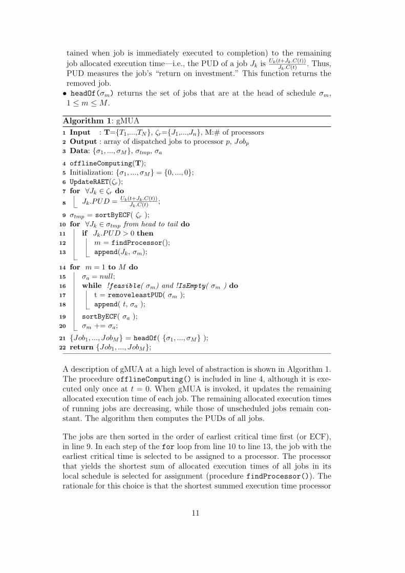
A description of gMUA at a high level of abstraction is shown in Algorithm 1.The procedure offlineComputing() is included in line 4, although it is exe-cuted only once at t = 0. When gMUA is invoked, it updates the remainingallocated execution time of each job. The remaining allocated execution timesof running jobs are decreasing, while those of unscheduled jobs remain con-stant. The algorithm then computes the PUDs of all jobs.

The jobs are then sorted in the order of earliest critical time first (or ECF),in line 9. In each step of the for loop from line 10 to line 13, the job with theearliest critical time is selected to be assigned to a processor. The processorthat yields the shortest sum of allocated execution times of all jobs in itslocal schedule is selected for assignment (procedure findProcessor()). Therationale for this choice is that the shortest summed execution time processor

11

results in the nearest scheduling event after assigning each job, and therefore,it establishes the same schedule as global EDF does. Then, the job Jk withthe earliest critical time is inserted into the local schedule σm of the selectedprocessor m.

In the for-loop from line 14 to line 20, gMUA attempts to make each localschedule feasible by removing the lowest PUD job. In line 16, if σm is notfeasible, then gMUA removes the job with the least PUD from σm until σmbecomes feasible. All removed jobs are temporarily stored in a schedule σaand then appended to each σm in ECF order. Note that simply aborting theremoved jobs may result in decreased accrued utility. This is because thealgorithm may decide to remove a job which is estimated to have a longerallocated execution time than its actual one, even though it may be able toattain utility. For this case, gMUA gives the job another chance to be scheduledinstead of aborting it, which eventually makes the algorithm more robust.Finally, each job at the head of σm, 1 ≤ m ≤ M is selected for execution onthe respective processor.

gMUA’s time cost depends upon that of procedures sortByECF(), findprocessor(),append(), feasible(), and removeLeastPUDJob(). With n tasks, sortByECF()costsO(nlogn). For SMPs with a restricted number of processors, findprocessor()’scostsO(M). While append() costsO(1) time, both feasible() and removeLeastPUDJob()

cost O(n). The while-loop in line 16 iterates at most n times, for an entireloop cost of O(n2). Thus, the algorithm costs O(Mn2). However, M of con-temporary SMPs is usually small (e.g., 16) and bounded with respect to theproblem size of number of tasks. Thus, gMUA costs O(n2).

gMUA’s O(n2) cost is similar to that of many past UA algorithms [6]. Ourprior implementation experience with UA scheduling at the middleware levelhas shown that the overhead is in the magnitude of sub-milliseconds [22] (sub-microsecond overheads may be possible at the kernel level). We anticipate asimilar overhead magnitude for gMUA. Though this cost is higher than that ofmany traditional algorithms, the cost is justified for applications with longerexecution time magnitudes such as those that we focus on here.

In traditional small scale static hard real-time subsystems, the task time scalesare usually microseconds to milliseconds to even a few seconds. For those timescales, the time overhead of a scheduling algorithm must be proportionatelylow. The time overhead of our many TUF/UA algorithms precludes softwareimplementations of them from being used in systems with mS-S time scales—although hardware (e.g., gate array) implementations can be used even downthere.

But our TUF/UA scheduling algorithms are intended for the many importanttime-critical applications in the gap between: classical real-time’s mS-S time

12

scales; and the classical logistics, job shop, etc. systems’ many minutes tomany hours time scales where proportionately higher cost general schedulingtheory, evolutionary algorithms, and linear programming are used.

The systems in that gap have time scales in the 1 S to few minutes range buttheir timeliness requirements are no less–and often more (cf. military combatsystems)—challenging and mission-critical than those of classical real-timesubsystems. These systems have adequate time for TUF/UA scheduling, andthose of interest to us need the benefits of it. 2

4 Algorithm Properties

4.1 Timeliness Assurances

We establish gMUA’s timeliness assurances under the conditions of (1) inde-pendent tasks that arrive periodically, and (2) task utilization demand satis-fies any of the feasible utilization bounds for global EDF (GFB, BAK, BCL)in [16].

Theorem 1 (Optimal Performance with Downward Step Shaped TUFs)Suppose that only downward step shaped TUFs are allowed under conditions(1) and (2). Then, a schedule produced by global EDF is also produced bygMUA, yielding equal accrued utilities. This is a critical time-ordered sched-ule.

PROOF. We prove this by examining Algorithm 1. In line 9, the queueσtmp is sorted in a non-decreasing critical time order. In line 12, the functionfindProcessor() returns the index of the processor on which the summedexecution time of assigned tasks is the shortest among all processors. Assumethat there are n tasks in the current ready queue. We consider two cases: (1)n ≤M and (2) n > M . When n ≤M , the result is trivial—gMUA’s scheduleof tasks on each processor is identical to that produced by EDF (every proces-sor has a single task or none assigned). When n > M , task Ti (M < i ≤ n) willbe assigned to the processor whose tasks have the shortest summed executiontime. This implies that this processor will have the earliest completion for allassigned tasks up to Ti−1, so that the event that will assign Ti will occur by

2 When UA scheduling is desired with lower overhead, solutions and tradeoffs ex-ist. Examples include linear-time stochastic UA scheduling [26], and using special-purpose hardware accelerators for UA scheduling (analogous to floating-point co-processors) [23].

13

this completion. Note that tasks in σtmp are selected to be assigned to pro-cessors according to ECF. This is precisely the global EDF schedule, as weconsider a TUFs critical time in UA scheduling to be the same as a deadlinein traditional hard real-time scheduling. Under conditions (1) and (2), EDFmeets all deadlines. Thus, each processor always has a feasible schedule, andthe while-block from line 16 to line 18 will never be executed. Thus, gMUAproduces the same schedule as global EDF.

Some important corollaries about gMUA’s timeliness behavior can be deducedfrom EDF’s behavior under conditions (1) and (2).

Corollary 2 Under conditions (1) and (2), gMUA always completes the al-located execution time of all tasks before their critical times.

Theorem 3 (Statistical Task-Level Assurance) Under conditions (1) and(2), gMUA meets the statistical timeliness requirement {νi, ρi} for each taskTi.

PROOF. From Corollary 2, all allocated execution times of tasks can becompleted before their critical times. Further, based on the results of Equa-tion 1, among the actual processor time of task Ti’s jobs, at least ρ′i (≥ ρi)of them have lesser actual execution time than the allocated execution time.Thus, gMUA can satisfy at least ρi critical times—i.e., the algorithm attainsνi utility with a probability of at least ρi.

Theorem 4 (System-Level Utility Assurance) Under conditions (1) and(2), if a task Ti’s TUF has the highest height Umax

i , then the system-level util-ity ratio, defined as the utility accrued by gMUA with respect to the system’s

maximum possible utility, is at leastρ1ν1Umax1 /P1+...+ρnνnUmaxn /Pn

Umax1 /P1+...+Umaxn /Pn.

PROOF. We denote the number of jobs released by task Ti as mi. Eachmi is computed as ∆t

pi, where ∆t is a time interval. Task Ti can attain at

least νi percentage of its maximum possible utility with the probability ρi.Thus, the ratio of the system-level accrued utility to the system’s maxi-mum possible utility is

ρ1ν1Umax1 m1+...+ρnνnUmaxn mnUmax1 m1+...+Umaxn mn

. Thus, the formula comes

toρ1ν1Umax1 /P1+...+ρnνnUmaxn /Pn

Umax1 /P1+...+Umaxn /Pn.

4.2 Dhall Effect

The Dhall effect [12] shows that there exists a task set that requires nearlyone total utilization demand, but cannot be scheduled to meet all deadlines

14

using global EDF even with infinite number of processors. Prior research hasrevealed that this is caused by the poor performance of global EDF when thetask set contains both high utilization tasks and low utilization tasks together.This phenomenon, in general, can also affect UA scheduling algorithms’ per-formance, and impede such algorithms’ ability to maximize the total accruedutility. We discuss this with an example inspired from [24]. We consider thecase when the execution time demands of all tasks are constant with no vari-ance, and gMUA estimates them accurately.

Example A. Consider M + 1 periodic tasks that are scheduled on M pro-cessors using global EDF. Let task Ti, where 1 ≤ i ≤ M , have pi = Di =1, Ci = 2ε, and task TM+1 have PM+1 = DM+1 = 1 + ε, CM+1 = 1. We assumethat each task Ti has a downward step shaped TUF with height hi and taskTM+1 has a downward step shaped TUF with height HM+1. When all tasksarrive at the same time, tasks Ti will execute immediately and complete theirexecution 2ε time units later. Task TM+1 then executes from time 2ε to time1 + 2ε. Since task TM+1’s critical time—we assume here it is the same as itsperiod—is 1 + ε, it begins to miss its critical time. By letting M →∞, ε→ 0,hi → 0 and HM+1 → ∞, we have a task set whose total utilization demandis near one and the maximum possible accrued utility is infinite, but whichfinally accrues zero utility even with infinite number of processors.

We call this phenomenon the UA Dhall effect. Conclusively, one of the reasonswhy global EDF is inappropriate as a UA scheduling algorithm is that it suffersthis effect. However, gMUA overcomes this phenomenon.

Example B. Consider the same scenario as in Example A, but now, let thetask set be scheduled by gMUA. In Algorithm 1, gMUA first tries to scheduletasks like global EDF, but it will fail to do so as we saw in Example A.When gMUA finds that TM+1 will miss its critical time on processor m (where1 ≤ m ≤M), the algorithm will select a task with lower PUD on processor mfor removal. On processor m, there should be two tasks, Tm and TM+1. Tm isone of Ti where 1 ≤ i ≤ M . When letting hi → 0 and HM+1 → ∞, the PUDof task Tm is almost zero and that of task TM+1 is infinite. Therefore, gMUAremoves Tm and eventually accrues infinite utility as expected.

In the case when the Dhall effect occurs, we can establish the UA Dhall effectby assigning extremely high utility to the task that will be selected and missits deadline using global EDF. This implies that the scheduling algorithmsuffering from the Dhall effect will likely suffer from UA Dhall effect, when itschedules the tasks that are subject to TUF time constraints.

The fact that gMUA is more robust against the UA Dhall effect than is globalEDF can be observed in our simulation experiments (see Section 5).

15

4.3 Sensitivity of Assurances

gMUA is designed under the assumption that tasks’ expected execution timedemands and the variances of the demands—i.e., the algorithm inputs E(Yi)and V ar(Yi)—are correct. However, it is possible that these inputs may havebeen miscalculated (e.g., due to errors in application profiling) or that theinput values may change over time (e.g., due to changes in the application’sexecution context). To understand gMUA’s behavior when this happens, weassume that the expected execution time demands, E(Yi)’s, and their vari-ances, V ar(Yi)’s, are erroneous, and develop the sufficient condition underwhich the algorithm is still able to meet {νi, ρi} for all tasks Ti.

Let a task Ti’s correct expected execution time demand be E(Yi) and itscorrect variance be V ar(Yi), and let an erroneous expected demand E ′(Yi)and an erroneous variance V ar′(Yi) be specified as the input to gMUA. Letthe task’s statistical timeliness requirement be {νi, ρi}. We show that if gMUAcan satisfy {νi, ρi} with the correct expectation E(Yi) and the correct varianceV ar(Yi), then there exists a sufficient condition under which the algorithm canstill satisfy {νi, ρi} even with the incorrect expectation E ′(Yi) and incorrectvariance V ar′(Yi).

Theorem 5 () Assume that gMUA satisfies {νi, ρi},∀i, under correct, ex-pected execution time demand estimates, E(Yi)’s, and their correct variances,V ar(Yi)’s. When incorrect expected values, E ′(Yi)’s, and variances, V ar′(Yi)’s,are given as inputs instead of E(Yi)’s and V ar(Yi)’s, gMUA satisfies {νi, ρi}, ∀i,if E ′(Yi) + (Ci − E(Yi))

√V ar′(Yi)V ar(Yi)

≥ Ci, ∀i, and the task execution time al-

locations, computed using E ′(Yi)’s and V ar′(Yi), satisfy any of the feasibleutilization bounds for global EDF.

PROOF. We assume that if gMUA has correct E(Yi)’s and V ar(Yi)’s asinputs, then it satisfies {νi, ρi},∀i. This implies that the Ci’s determined byEquation 1 are feasibly scheduled by gMUA satisfying all task critical times:

ρi =(Ci − E(Yi))

2

V ar(Yi) + (Ci − E(Yi))2. (2)

However, gMUA has incorrect inputs, E ′(Yi)’s and V ar′(Yi), and based onthose, it determines C ′is by Equation 1 to obtain the probability ρi,∀i:

ρi =(C ′i − E ′(Yi))2

V ar′(Yi) + (C ′i − E ′(Yi))2. (3)

16

Unfortunately, C ′i that is calculated from the erroneous E ′(Yi) and V ar′(Yi)leads gMUA to another probability ρ′i by Equation 1. Thus, although we ex-pect assurance with the probability ρi, we can only obtain assurance with theprobability ρ′i because of the error. ρ′ is given by:

ρ′i =(C ′i − E(Yi))

2

V ar(Yi) + (C ′i − E(Yi))2. (4)

Note that we also assume that tasks with C ′i satisfy the global EDF’s uti-lization bound; otherwise gMUA cannot provide the assurances. To satisfy{νi, ρi}, ∀i, the actual probability ρ′i must be greater than the desired proba-bility ρi. Since ρ′i ≥ ρi,

(C ′i − E(Yi))2

V ar(Yi) + (C ′i − E(Yi))2≥ (Ci − E(Yi))

2

V ar(Yi) + (Ci − E(Yi))2.

Hence, C ′ ≥ Ci. From Equations 2 and 3,

C ′i = E ′(Yi) + (Ci − E(Yi))

√√√√V ar′(Yi)V ar(YI)

≥ Ci. (5)

Corollary 6 () Assume that gMUA satisfies {νi, ρi},∀i, under correct, ex-pected execution time demand estimates, E(Yi)’s, and their correct variances,V ar(Yi)’s. When incorrect expected values, E ′(Yi)’s, are given as inputs insteadof E(Yi)’s but with correct variances V ar(Yi), gMUA satisfies {νi, ρi}, ∀i, ifE ′(Yi) ≥ E(Yi),∀i, and the task execution time allocations, computed usingE ′(Yi)’s, satisfy the feasible utilization bound for global EDF.

PROOF. This can be proved by replacing V ar′(Yi) with V ar(Yi) in Equa-tion 5.

Corollary 6, a special case of Theorem 5, is intuitively straightforward. Itessentially states that if overestimated demands are feasible, then gMUA canstill satisfy {νi, ρi},∀i. Thus, it is desirable to specify larger E ′(Yi)s as inputto the algorithm when there is the possibility of errors in determining theexpected demands, or when the expected demands may vary with time.

Corollary 7 () Assume that gMUA satisfies {νi, ρi},∀i, under correct, ex-pected execution time demand estimates, E(Yi)’s, and their correct variances,V ar(Yi)’s. When incorrect variances, V ar′(Yi)’s, are given as inputs insteadof correct V ar(Yi)’s but with correct expectations E(Yi)’s, gMUA satisfies{νi, ρi}, ∀i, if V ar′(Yi) ≥ V ar(Yi),∀i, and the task execution time allocations,computed using E ′(Yi)’s, satisfy the feasible utilization bound for global EDF.

17

PROOF. This can be proved by replacing E ′(Yi) with E(Yi) in Equation 5.

5 Experimental Evaluation

We conducted simulation-based experimental studies to validate our analyticalresults, and to compare gMUA’s performance with global EDF. We take theglobal EDF algorithm as our counterpart since it is one of the global schedul-ing algorithms, like gMUA, that allows full migration and does not depend ontime quanta. Note that gMUA uses deadline time constraints as opposed togMUA which uses TUF time constraints. We consider two cases: (1) the de-mand of all tasks is constant (i.e., zero variance) and gMUA exactly estimatestheir execution time allocation, and (2) the demand of all tasks statisticallyvaries and gMUA probabilistically estimates the execution time allocation foreach task. The former experiment is conducted to evaluate gMUA’s genericperformance as opposed to EDF, while the latter is conducted to validatethe algorithm’s assurances. The experiments focus on the no dependency case(i.e., each task is assumed to be independent of others).

5.1 Performance with Constant Demand

We consider an SMP machine with four processors. A task Ti’s period pi(= tXi )and its expected execution times E(Yi) are randomly generated with uniformdistribution in the range [1,30] and [1, α·pi], respectively, where α is defined asmax{Ci

pi|i = 1, ..., n} and V ar(Yi) are zero. According to [14], EDF’s feasible

utilization bound depends on α as well as the number of processors. It impliesthat no matter how many processors the system has, there exist task sets withtotal utilization demand (UD) close to one, which cannot be scheduled to sat-isfy all deadlines using EDF. Generally, the performance of global schedulingalgorithms tends to decrease when α increases.

We consider two TUF shape patterns: (1) a homogeneous TUF class in whichall tasks have downward step shaped TUFs, and (2) a heterogeneous TUFclass, including downward step, linearly decreasing, and parabolic shapes.Each TUF’s height is randomly generated in the range [1,100].

The number of tasks is determined depending on the given UD and the αvalue. We vary the UD from 3 to 6.5, including the case where it exceeds thenumber of processors. We set α to 0.4, 0.7, and 1. For each experiment, morethan 1,000,000 jobs are released. To see the generic performance of gMUA, weassume {νi, ρi} = {0, 1}.

18

2.5 3.0 3.5 4.0 4.5 5.0 5.5 6.0 6.5 7.00

20

40

60

80

100

AU

R (%

)

Utilization Demand (UD)

gMUA ( =0.4) gMUA ( =0.7) gMUA ( =1.0) EDF ( =0.4) EDF ( =0.7) EDF ( =1.0)

(a) AUR

2.5 3.0 3.5 4.0 4.5 5.0 5.5 6.0 6.5 7.00

20

40

60

80

100

CM

R (%

)

Utilization Demand (UD)

gMUA ( =0.4) gMUA ( =0.7) gMUA ( =1) EDF ( =0.4) EDF ( =0.7) EDF ( =1)

(b) CMR

Fig. 3. Performance Under Constant Demand, Step TUFs

Figures 3 and 4 show the accrued utility ratio (AUR) and critical-time meetratio (CMR) of gMUA and EDF, respectively, under increasing UD (from 3.0to 6.5) and for the three α values. AUR is the ratio of total accrued utilityto the total maximum possible utility, and CMR is the ratio of the numberof jobs meeting their critical times to the total number of job releases. For atask with a downward step TUF, its AUR and CMR are identical. But thesystem-level AUR and CMR can be different due to the mix of different taskutilities.

2.5 3.0 3.5 4.0 4.5 5.0 5.5 6.0 6.5 7.00

20

40

60

80

100

AU

R (%

)

Utilization Demand (UD)

gMUA ( =0.4) gMUA ( =0.7) gMUA ( =1) EDF ( =0.4) EDF ( =0.7) EDF ( =1)

(a) AUR

2.5 3.0 3.5 4.0 4.5 5.0 5.5 6.0 6.5 7.00

20

40

60

80

100

CM

R (%

)

Utilization Demand (UD)

gMUA ( =0.4) gMUA ( =0.7) gMUA ( =1) EDF ( =0.4) EDF ( =0.7) EDF ( =1)

(b) CMR

Fig. 4. Performance Under Constant Demand, Heterogeneous TUFs

When all tasks have downward step TUFs and the total UD satisfies the globalEDF’s feasible utilization bound, gMUA performs exactly the same as EDF.This validates Theorem 1.

EDF’s performance drops sharply after UD = 4.0 (for downward step TUFs),which corresponds to the number of processors in our experiments. This is dueto EDF’s domino effect (originally identified for single processors) that occurshere, when UD exceeds the number of processors. On the other hand, theperformance of gMUA gracefully degrades as UD increases and exceeds 4.0,since gMUA selects as many feasible, higher PUD tasks as possible, insteadof simply favoring earlier deadline tasks.

19

Observe that EDF begins to miss deadlines much earlier than when UD = 4.0,as indicated in [16]. Even when UD < 4.0, gMUA outperforms EDF in bothAUR and CMR. This is because gMUA is likely to find a feasible or at leastbetter schedule even when EDF cannot find a feasible one, as we have seen inSection 4.2.

We also observe that α affects the AUR and CMR of both EDF and gMUA.Despite this effect, gMUA outperforms EDF for the same α and UD for thereason that we describe above.

We observe similar and consistent trends for tasks with heterogeneous TUFs inFigure 4. The figure shows that gMUA is superior to EDF with heterogeneousTUFs and when UD exceeds the number of processors.

5.2 Performance with Statistical Demand

We now evaluate gMUA’s statistical timeliness assurances. The task settingsused in our simulation study are summarized in Table 1. The table shows thetask periods and the maximum utility (or Umax) of the TUFs. For each taskTi’s demand Yi, we generate normally distributed execution time demands.Task execution times are changed along with the total UD. We consider bothhomogeneous and heterogeneous TUF shapes as before.

Table 1Task Settings

Task pi Umaxi ρi E(Yi) V ar(Yi)

T1 25 400 0.96 3.15 0.01

T2 28 100 0.96 13.39 0.01

T3 49 20 0.96 18.43 0.01

T4 49 100 0.96 23.91 0.01

T5 41 30 0.96 14.98 0.01

T6 49 400 0.96 24.17 0.01

Figure 5(a) shows AUR and CMR of each task under increasing total UD ofgMUA. For a task with downward step TUFs, task-level AUR and CMR areidentical, as satisfying the critical time implies the attainment of a constantutility. But the system-level AUR and CMR are different as satisfying thecritical time of each task does not always yield the same amount of utility.

Figure 5(a) shows that all tasks scheduled by gMUA accrue 100% AUR andCMR within the global EDF’s bound (i.e., UD<≈2.5 here), thus satisfying

20

3 4 5 6 7 8 9

0

20

40

60

80

100

AU

R (=

CM

R) (

%)

Utilization Demand (UD)

T1 T2 T3 T4 T5 T6

(a) Task-level

2 3 4 5 6 7 8 9 100

20

40

60

80

100

AU

R a

nd C

MR

(%)

Utilization Demand (UD)

AUR CMR

(b) System-level

Fig. 5. Performance Under Statistical Demand, Step TUFs

the desired {νi, ρi} = {1, 0.96},∀i. This validates Theorem 3.

Under the condition beyond what Theorem 3 indicates, gMUA achieves grace-ful performance degradation in both AUR and CMR in Figure 5(b), as theprevious experiment in Section 5.1 implies. In Figure 5(a), gMUA achieves100% AUR and CMR for T1 over the whole range of UD. This is because T1

has a downward step TUF with higher height. Thus, gMUA favors T1 overothers to obtain more utility when it cannot satisfy the critical time of alltasks.

According to Theorem 4, the system-level AUR must be at least 96%. (Foreach task Ti, νi = 1, because all TUFs are downward step shaped.) We observethat AUR and CMR of gMUA under the condition of Theorem 4 are above99.0%. This validates Theorem 4.

2 3 4 5 6 7 8 90

20

40

60

80

100

AU

R (%

)

Utilization Demand (UD)

T1 T2 T3 T4 T5 T6

(a) Task-level

2 3 4 5 6 7 8 9 100

20

40

60

80

100

AU

R a

nd C

MR

(%)

Utilization Demand (UD)

AUR CMR

(b) System-level

Fig. 6. Performance Under Statistical Demand, Heterogenous TUFs

A similar trend is observed in Figure 6 for heterogeneous TUFs. We as-sign downward step TUFs for T1 and T4, linearly decreasing TUFs for T2

and T5, and parabolic TUFs for T3 and T6. For each task Ti, νi is set as{1.0, 0.1, 0.1, 1.0, 0.1, 0.1}.

According to Theorem 4, the system-level AUR must be at least 0.96 ×

21

(400/25+100×0.1/28+20×0.1/49+100/49+30×0.1/41+400×0.1/49)/(400/25+100/28 + 20/49 + 100/49 + 30/41 + 400/49) = 62.5%. In Figure 6, we observethat the system-level AUR under gMUA is above 62.5%. This further validatesTheorem 4 for non step-shaped TUFs. We also observe that the system-levelAUR and CMR of gMUA degrade gracefully, since gMUA favors as manyfeasible, high PUD tasks as possible.

6 Conclusions and Future Work

We present a global TUF/UA scheduling algorithm for SMPs, called gMUA.The algorithm applies to tasks that are subject to TUF time constraints,variable execution time demands, and resource overloads. gMUA has the two-fold scheduling objective of probabilistically satisfying utility lower bounds foreach task, and maximizing the accrued utility for all tasks.

We establish that gMUA achieves optimal accrued utility for the special caseof downward step TUFs and when the total task utilization demand doesnot exceed global EDF’s feasible utilization bound. Further, we prove thatgMUA probabilistically satisfies task utility lower bounds, and lower boundsthe system-wide accrued utility. We also show that the algorithm’s utilitylower bound satisfactions have bounded sensitivity to variations in executiontime demand estimates, and that the algorithm is robust against a variant ofthe Dhall effect. When task utility lower bounds cannot be satisfied (due toincreased utilization demand), gMUA maximizes the accrued utility.

Our simulation experiments validate our analytical results and confirm thealgorithm’s effectiveness. Our method of transforming task stochastic demandinto actual task execution time allocation is independent of gMUA, and canbe applied in other algorithmic contexts, where similar (stochastic scheduling)problems arise.

Some aspects of our work lead to directions for further research. Examplesinclude relaxing the sporadic task arrival model to allow a stronger adversary(e.g., the unimodal arbitrary arrival model), allowing greater task utilizationsfor satisfying utility lower bounds, and reducing the algorithm overhead.

Acknowledgements

This work was supported by the U.S. Office of Naval Research under GrantN00014-00-1-0549 and by The MITRE Corporation under Grant 52917. E.

22

Douglas Jensen was supported by the MITRE Technology Program. A pre-liminary version of this paper appeared as “On Multiprocessor Utility AccrualReal-Time Scheduling With Statistical Timing Assurances,” H. Cho, H. Wu,B. Ravindran, and E. D. Jensen, 2006 IFIP International Conference on Em-bedded And Ubiquitous Computing (EUC), August 01-04, 2006, Seoul, Korea.

References

[1] R. K. Clark, E. D. Jensen, N. F. Rouquette, ”Software organization to facilitatedynamic processor scheduling,” IEEE WPDRTS, pp.122, April, 2004.

[2] R. K. Clark, E. D. Jensen, and others, ”An Adaptive, Distributed AirborneTracking System,” IEEE WPDRTS, pp.353-362, April, 1999.

[3] C. L. Liu, J. W. Layland, ”Scheduling Algorithms for Multiprogramming ina Hard Real-Time Environment,” Journal of the ACM, vol.20, no.1, pp.46-61,1973.

[4] E. D. Jensen, C. D. Locke, H. Tokuda, ”A Time-Driven Scheduling Model forReal-Time Systems”, IEEE RTSS, pp.112-122, Dec., 1985.

[5] D. P. Maynard, S. E. Shipman and others, ”An Example Real-Time Command,Control, and Battle Management Application for Alpha,” Archons Project TR88121, CMU CS Dept., Dec. 1988.

[6] B. Ravindran, E. D. Jensen, P. Li, ”On Recent Advances in Time/UtilityFunction Real-Time Scheduling and Resource Management,” , IEEE ISORC,pp.55-60, May, 2005.

[7] QNX, ”Symmetric Multiprocessing”, http://www.qnx.com/products/rtos/smp.html, Last accessed October 2005.

[8] Yu-Kwong Kwok and Ishfaq Ahmad, ”Static Scheduling Algorithms forAllocating Directed Task Graphs to Multiprocessors,” ACM ComputingSurveys, vol. 31, no. 4, pp. 406-471, December 1999.

[9] J. Carpenter, S. Funk and others, ”A categorization of real-time multiprocessorscheduling problems and algorithms”, Handbook on Scheduling Algorithms,Methods, and Models, pp.30.1-30.19, Chapman Hall/CRC, 2004.

[10] S. Baruah, N. Cohen, C. G. Plaxton, D. Varvel, ”Proportionate Progress: ANotion of Fairness in Resource Allocation,” Algorithmica, vol.15, pp.600, 1996.

[11] U. C. Devi, J. Anderson, ”Tardiness Bounds for Global EDF Scheduling on aMultiprocessor,” IEEE RTSS, pp.330-341, 2005.

[12] S. K. Dhall, C. L. Liu, ”On a real-time scheduling problem,” OperationsResearch, vol.26, no.1, 1978.

23

[13] A. Srinivasan, S. Baruah, ”Deadline-based Scheduling of Periodic Task Systemson Multiprocessors”, Information Processing Letters, pp.93-98, Nov. 2002.

[14] J. Goossens, S. Funk, S. Baruah, ”Priority-Driven Scheduling of Periodic TasksSystems on Multiprocessors,” Real-Time Systems, vol.25, no.2-3, pp.187-205,2003.

[15] T. P. Baker, ”Multiprocessor EDF and Deadline Monotonic SchedulabilityAnalysis,” IEEE RTSS, pp.120-129, Dec., 2003.

[16] M. Bertogna, M. Cirinei, G. Lipari, ”Improved Schedulability Analysis of EDFon Multiprocessor Platforms,” IEEE ECRTS, pp.209-218, 2005.

[17] A. Srinivasan, J. Anderson, ”Efficient scheduling of soft real-time applicationson multiprocessors,” IEEE ECRTS, pp.51-59, July, 2003.

[18] Philip Holman, James H. Anderson, ”Adapting Pfair Scheduilng for SymmetricMultiprocessors”, Journal of Embedded Computing, to appear.

[19] H. Aydin, R. Melhem, D. Mosse, P. Mejia-Alvarez, ”Dynamic and aggressivescheduling techniques for power-aware real-time systems,” IEEE RTSS, pp.95-105, Dec., 2001.

[20] X. Zhang, Z. Wang, and others, ”System support for automated profiling andoptimization,” ACM SOSP, pp.15-26, Oct., 1997.

[21] R. K. Clark, ”Scheduling Dependent Real-Time Activities”, Carnegie MellonUniversity, 1990.

[22] P. Li, B. Ravindran, and others, ”A Formally Verified Application-LevelFramework for Real-Time Scheduling on POSIX Real-Time OperatingSystems,” IEEE Trans. Software Engineering, vol.30, no.9, pp.613-629, Sept.,2004.

[23] J. D. Northcutt, ”Mechanisms for Reliable Distributed Real-Time OperatingSystems – The Alpha Kernel,” Academic Press, 1987.

[24] O. U. P. Zapata, P. M. Alvarez, ”EDF and RM MultiprocessorScheduling Algorithms: Survey and Performance Evaluation,” http://delta.cs.cinvestav.mx/~pmejia/multitechreport.pdf, Last accessed October2005.

[25] J. Anderson, V. Bud, U. C. Devi, ”An EDF-based Scheduling Algorithm forMultiprocessor Soft Real-Time Systems,” IEEE ECRTS, pp.199-208, July, 2005.

[26] P. Li, B. Ravindran, ”A POSIX RTOS-based Middleware for Soft Real-TimeDistributed Systems,” Proceedings of The IEEE International Parallel andDistributed Processing Symposium, April, 2004.

24