Utilising carbon dioxide for transport fuels : the

This is a repository copy of Utilising carbon dioxide for transport fuels : the economic and environmental sustainability of different Fischer-Tropsch process designs.

White Rose Research Online URL for this paper:http://eprints.whiterose.ac.uk/150830/

Version: Published Version

Article:

Cuéllar-Franca, R., García-Gutiérrez, P., Dimitriou, I. et al. (3 more authors) (2019) Utilising carbon dioxide for transport fuels : the economic and environmental sustainability of different Fischer-Tropsch process designs. Applied Energy, 253. ISSN 0306-2619

https://doi.org/10.1016/j.apenergy.2019.113560

[email protected]://eprints.whiterose.ac.uk/

Reuse

This article is distributed under the terms of the Creative Commons Attribution (CC BY) licence. This licence allows you to distribute, remix, tweak, and build upon the work, even commercially, as long as you credit the authors for the original work. More information and the full terms of the licence here: https://creativecommons.org/licenses/

Takedown

If you consider content in White Rose Research Online to be in breach of UK law, please notify us by emailing [email protected] including the URL of the record and the reason for the withdrawal request.

mailto:[email protected]

https://eprints.whiterose.ac.uk/

Contents lists available at ScienceDirect

Applied Energy

journal homepage: www.elsevier.com/locate/apenergy

Utilising carbon dioxide for transport fuels: The economic andenvironmental sustainability of different Fischer-Tropsch process designs

Rosa Cuéllar-Francaa,⁎, Pelayo García-Gutiérreza, Ioanna Dimitrioub, Rachael H. Elderb,Ray W.K. Allenb, Adisa Azapagica

a School of Chemical Engineering and Analytical Science, The Mill, Sackville Street, The University of Manchester, Manchester M13 9PL, UKbDepartment of Chemical and Biological Engineering, Mappin Street, University of Sheffield, Sheffield S1 3JD, UK

H I G H L I G H T S

• For large-scale plants, CO2-derivedfuels outperform diesel en-vironmentally.

• The exceptions are global warmingand ozone depletion which are lowerfor diesel.

• Optimising the systems reduces globalwarming of CO2 fuels by 70% belowdiesel.

• CO2 fuels are not economically viable,costing ∼4 times more than fossildiesel.

• Optimising process yields would allowdecreasing the subsidies to 8%.

G R A P H I C A L A B S T R A C T

A R T I C L E I N F O

Keywords:Carbon capture and utilisationClimate changeFischer-Tropsch liquid fuelsLife cycle assessmentLife cycle costingSustainability assessment

A B S T R A C T

Producing fuels and chemicals from carbon dioxide (CO2) could reduce our dependence on fossil resources andhelp towards climate change mitigation. This study evaluates the sustainability of utilising CO2 for production oftransportation fuels. The CO2 feedstock is sourced from anaerobic digestion of sewage sludge and the fuels areproduced in the Fischer-Tropsch (FT) process. Using life cycle assessment, life cycle costing and profitabilityanalysis, the study considers four different process designs and a range of plant capacities to explore the effect ofthe economies of scale. For large-scale plants (1,670 t/day), the FT fuels outperform fossil diesel in all en-vironmental impacts across all the designs, with several impacts being net-negative. The only exceptions areozone depletion, for which fossil diesel is the best option, and global warming potential (GWP), which is lowerfor fossil diesel for some process designs. Optimising the systems reduces the GWP of FT fuels in the best case by70% below that of fossil diesel. Assuming a replacement of 9.75–12.4% of fossil diesel consumed in the UK by2,032, as stipulated by policy, would avoid 2–8 Mt of CO2 eq./yr, equivalent to 2–8% of annual emissions fromtransportation. However, these fuels are not economically viable and matching diesel pump price would requiresubsidies of 35–79% per litre. Optimising production yields would allow decreasing the subsidies to 8%. Futureresearch should be aimed at technology improvements to optimise these systems as well as evaluating differentpolicy mechanisms needed to stimulate markets for CO2-derived fuels.

https://doi.org/10.1016/j.apenergy.2019.113560Received 16 April 2019; Received in revised form 12 July 2019; Accepted 15 July 2019

⁎ Corresponding author.E-mail address: [email protected] (R. Cuéllar-Franca).

Applied Energy 253 (2019) 113560

Available online 05 September 20190306-2619/ © 2019 The Authors. Published by Elsevier Ltd. This is an open access article under the CC BY license (http://creativecommons.org/licenses/BY/4.0/).

T

http://www.sciencedirect.com/science/journal/03062619

https://www.elsevier.com/locate/apenergy



mailto:[email protected]


http://crossmark.crossref.org/dialog/?doi=10.1016/j.apenergy.2019.113560&domain=pdf

1. Introduction

Our dependence on fossil fuels is depleting abiotic resources andcontributing to climate change [1]. While substantial reductions inconsumption are paramount, research efforts to produce fuels fromalternative feedstocks must continue. One such feedstock is carbon di-oxide (CO2). While CO2 is already being utilised for production ofchemicals, such as urea, methanol and polyols [2,3], the overall con-sumption of CO2 as a feedstock by the chemicals industry is below 1%of the 49.3 Gt/yr of anthropogenic CO2 emitted globally [4]. Therefore,CO2 utilisation strategies should encourage and prioritise the produc-tion of products with high demand, such as transportation fuels [5].This paper focuses on utilisation of CO2 to produce liquid transportfuels via Fischer-Tropsch (FT) synthesis with the aim of finding out ifsuch fuels would be environmentally and economically sustainable on alife cycle basis relative to fossil and renewable fuels.

Production of liquid fuels via FT synthesis is a well-establishedpractice in industry. However, the feedstocks are largely derived fromfossil resources, such as coal or natural gas, particularly in countrieswith limited reserves of crude oil [6,7]. For example, Sasol in SouthAfrica produces synthetic liquid fuels from coal [8], while ExxonMobilin Qatar [7] and Shell in Malaysia rely on their large natural gas re-serves for the production of liquid fuels [5]. In FT synthesis, syngas(carbon monoxide and hydrogen) is converted into a mixture of gaseousand liquid hydrocarbon fuels through a catalyst-aided polymerisationreaction [9]. Although syngas is commonly produced from coal gasifi-cation or steam reforming of natural gas, alternative feedstocks, such asbiomass or CO2, can be used for the production of syngas [5,6,9].

2. Literature review

Over the last decade, several studies evaluated techno-economicfeasibility and/or environmental performance of the production of FTliquid fuels from different fossil and renewable feedstocks. For anoverview of these studies, see Table 1. Dry [6] and Jaramillo et al. [7]compared the economic viability of different pathways for producingFT fuels from coal and natural gas in South Africa and the United States,respectively. Both studies concluded that the profitability of FT plantsdepended highly on crude oil prices, carbon taxes and feedstock prices.For example, it was found that FT fuels from natural gas could onlycompete with conventional fossil fuels at low gas prices ($0.5 per mil-lion cubic feet) and high crude oil prices ($120 per barrel). Conversely,at low crude oil prices ($40 per barrel), neither coal-nor gas-derived FTfuels were economically competitive. On the other hand, Jaramilloet al. [7] found that both types of FT fuels could achieve greenhouse gasemissions (GHG) comparable to fossil fuels (87 vs 85 g CO2 eq./MJ), butonly under very optimistic scenarios, involving carbon capture and

storage and low-carbon electricity sources. Most recently, Liu et al. [10]evaluated the economic and GHG emissions of coal and biomass to li-quid (CBTL) processes with carbon capture and storage (CCS) for theproduction of liquid fuels. According to this study, both price and GHGemissions highly depended on regional biomass availability as thisdetermined the optimum biomass-to-coal ratio. It was determined thatthe ratio of 8/92 provided the best balance between price and GHGreductions estimated at 56 pence per litre and 93.6 g CO2 eq./MJ, re-spectively [10].

Although FT fuels from renewable feedstocks were found generallyto be more favourable than from fossil resources with respect to lifecycle GHG emissions, the latter ranged widely from −20 to 150 g CO2

eq./MJ of fuel, depending on the unit of analysis, system boundaries,assumptions and allocation methods. For example, some studies ex-cluded transport and pre-treatment of the feedstock [11], while othersexcluded the use (combustion) of fuels [12].

Some studies considered specifically techno-economic feasibilityand/or environmental implications of CO2-derived liquid fuels. Thosemost relevant to this work are summarised in Table 2; for further detailson the production pathways and costs, see Graves et al. [13] and Bry-nolf et al. [14], respectively. For example, Abanades et al. [15] assessedthe avoided CO2 emissions and related mitigation costs of a CO2-to-methanol process. The study showed that this particular carbon captureand utilisation (CCU) system was no better than producing methanolfrom fossil resources in terms of climate change mitigation and waseven more costly. On the other hand, Deutz et al. [16] found thatblending diesel with CO2-derived oxymethylene ethers could reduce theGHG emissions from transport fuels by 22% if hydrogen was producedvia water electrolysis using renewable energy. In addition to GHGemissions, this study also estimated the emissions of NOx and particu-lates from fuel combustion. Hombach et al. [17] also looked at theproduction of hydrogen via two different water electrolysis technolo-gies using fossil and renewable energy for the production of FT liquidfuel from CO2 captured from air considering current (2015) and futureprojections (2030). The estimated global warming potential (GWP)varied between 64 and 440 g CO2 eq. per MJ of FT liquid fuels for thecurrent situation, and 7–150 g CO2 eq./MJ for the future scenario, de-pending on the electrolysis technology and energy source. The pro-duction costs for all cases were found to be 3–5 times higher than thepump price of fossil diesel in Germany. Van der Giesen et al. [18] alsoestimated the GWP of the production of FT liquid fuels from CO2 cap-tured from three different sources: combustion of woodchips, combus-tion of natural gas and direct air capture. Similarly to Hombach et al.[17], the results ranged from 30 to 290 g CO2 eq. per MJ of fuels, de-pending on the CO2 and energy sources. Overall, the direct air captureprocess powered by solar electricity was the best option with respect tothe GWP. Solar energy was also considered in a techno-economic

Nomenclature

Aj, avg annual cash flow (£/y)Ax non-manufacturing fixed-capital investment (£)C1 capacity of a base-case plant (t/day)C2 capacity of a scaled-up plant (t/day)CO&Mavg average annual operating and maintenance costs (£/yr)d annual depreciation (£/y)GPavg average annual gross profit over the lifetime of the plant

(£/yr)m annual production of liquid fuels (l/yr)MARR minimum annual acceptable rate of return on investment

(%/yr)

N evaluation period (years)n length of the straight-line recovery periodNPavg average annual net profit over the lifetime of the plant

(£/yr)p basic price of liquid fuels (pence/l)PBP payback period (yr)Savg average annual revenue from fuel sales over the lifetime of

the plant (£/yr)TCI total capital investment (£)TCI1 total capital investment for a base-case plant (£)TCI2 total capital investment for a scaled-up plant (£)V manufacturing fixed-capital investment (£)Φ income tax (%)

R. Cuéllar-Franca, et al. Applied Energy 253 (2019) 113560

2

analysis of the production of FT liquid fuels in comparison with pro-duction of methanol from fossil-derived CO2 [19]. The results indicatedthat the capital investment and operating and maintenance costs re-quired for the FT plant were 2.3 times lower than for the methanolplant.

Furthermore, three studies assessed the economic viability of usingbiogas from sewage sludge to produce FT liquid fuels [5,20,21]. How-ever, they varied in scope. For example, Badgett et al. [20] estimatedthe potential feedstock prices of various organic waste sources, in-cluding sewage sludge, based on the associated costs of their treatmentand disposal. The study concluded that sewage sludge could be avail-able at low or negative prices depending on local regulations. Her-nandez and Martin [21] went beyond the feedstocks to determine thecosts of producing FT fuels from sewage-derived biogas. The authorssuggested that the production costs could potentially compete withcurrent selling prices of fossil fuels if ‘sustainability tax allowances’were introduced. Dimitriou et al. [5] also considered costs of producingFT fuels from biogas, comparing different process configurations on fuelyields, energy requirements, capital investment and production costs.The results suggested that the production of liquid fuels via FT was noteconomically feasible, mainly because of the low CO2 separation andconversion efficiencies as well as the high energy requirements [5].However, the study did not consider full life cycle costs, focusing onlyon the production costs.

Similarly, none of the previous studies considered the full life cyclecosts or environmental impacts either. Furthermore, no study of FTfuels derived from CO2 considered any other environmental impactsbeyond the GWP (Table 2). This work goes beyond the state-of-the-artto provide a comprehensive evaluation of the life cycle economic andenvironmental sustainability of the production and consumption of FTliquid fuels derived from CO2, with the aim of identifying the mostpromising designs for potential deployment. Life cycle assessment(LCA), life cycle costing (LCC) and profitability analysis have been usedfor these purposes. The last goes beyond production costs to estimatepotential selling prices of fuels. Four representative FT process designsare considered, using CO2 emitted in anaerobic digestion of sewagesludge during production of biogas, therefore, exploring an alternativeand possibly a more profitable application of sludge, which is currentlyused only as fertiliser. This is described in the next section, alongsidethe data and assumptions used in the study. The results of the en-vironmental and economic evaluations are presented in Section 4, to-gether with the scale-up of the plants and various sensitivity analyses.Possible policy implications related to these fuels are also considered inthis section. The conclusions and recommendations for policy and fu-ture work are given in Section 5.

3. Methods

3.1. Process description

This study considers four process designs (PD) for the production ofFT fuels from sewage sludge proposed previously by the authors [5]. Alldesigns rely on the best available and proven technologies for CCU andare ready for deployment. They differ in the methods used to separateand capture the CO2 present in the biogas, as follows:

(i) PD-MEA: CO2 capture from raw (‘unsweetened’) biogas by ab-sorption in monoethanolamine (MEA);

(ii) PD-CHP1: combustion of unsweetened biogas in a combined heatand power (CHP) and utilisation of CO2 present in flue gases;

(iii) PD-CHP2 (combination of PD-MEA and PD-CHP1): MEA CO2

capture from unsweetened biogas and utilisation of CO2 from fluegases generated in combustion of sweetened biogas in a CHP plant;and

(iv) PD-CHP3: MEA CO2 capture from flue gas generated by combus-tion of unsweetened biogas in a CHP plant.T

able1

Sum

mar

yof

econ

omic

and

envi

ronm

enta

las

sess

men

tst

udie

sof

Fisc

her-

Trop

sch

(FT)

liqui

dfu

els.

Stud

yCou

ntry

Scop

eFe

edst

ock

Uni

tof

anal

ysis

Syst

embo

unda

ries

Econ

omic

asse

ssm

ent

Envi

ronm

enta

las

sess

men

t

Dry

[6]

Sout

hA

fric

aR

evie

wof

FTpr

oces

ses

for

the

prod

ucti

onof

dies

elan

dth

eec

onom

icvi

abili

tyof

exis

ting

FTpl

ants

Coa

lan

dna

tura

lga

sU

SDpe

rba

rrel

Cra

dle

toga

teEc

onom

icvi

abili

tyof

exis

ting

FTpl

ants

–

Jara

mill

oet

al.[7

]U

SAEn

viro

nmen

talan

dec

onom

icas

sess

men

tof

prod

ucti

onof

FTliq

uid

fuel

sCoa

lan

dna

tura

lga

sLi

tres

offu

elCra

dle

togr

ave

Tech

no-e

cono

mic

asse

ssm

ent

ofCTL

and

GTL

plan

tsa

Life

cycl

eG

HG

emis

sion

s

Wan

get

al.[1

2]U

SAEn

viro

nmen

talan

dec

onom

icop

tim

isat

ion

ofhy

droc

arbo

nbi

orefi

nery

for

prod

ucti

onof

FTliq

uid

fuel

s

Cel

lulo

sic

biom

ass

Gas

olin

eeq

uiva

lent

gallo

nsG

ate

toga

teN

etpr

esen

tva

lue

ofa

bior

efine

ryG

loba

lw

arm

ing

pote

ntia

l

Pres

sley

etal

.[2

2]U

SAEn

viro

nmen

talas

sess

men

tof

prod

ucti

onof

FTliq

uid

fuel

sin

are

fuse

-der

ived

fuel

faci

lity

Mun

icip

also

lidw

aste

One

met

ric

tonn

eof

mix

edw

aste

Cra

dle

togr

ave

–G

loba

lw

arm

ing

pote

ntia

l

Ahm

adiM

ogha

ddam

etal

.[1

1]Sw

eden

Com

pari

son

ofen

viro

nmen

talpe

rfor

man

ceof

alte

rnat

ive

biog

as-d

eriv

edfu

els,

incl

udin

gFT

dies

el

Biog

asN

orm

alcu

bic

met

ers

ofra

wbi

ogas

Gat

eto

grav

e(e

xclu

des

anae

robi

cdi

gest

ion

for

biog

aspr

oduc

tion

)

–G

loba

lw

arm

ing

pote

ntia

l

Pete

rsen

etal

.[2

3]So

uth

Afr

ica

Com

pari

son

ofen

viro

nmen

talpe

rfor

man

ceof

alte

rnat

ive

biom

ass-

deri

ved

fuel

s,in

clud

ing

FTdi

esel

Suga

rcan

eba

gass

eFu

elre

quir

edto

trav

el1

kmCra

dle

togr

ave

–G

loba

lw

arm

ing

pote

ntia

l,de

plet

ion

ofab

ioti

cre

sour

ces,

acid

ifica

tion

,eu

trop

hica

tion

,hum

anto

xici

tyLi

uet

al.[1

0]U

SAEn

viro

nmen

talan

dec

onom

icfe

asib

ility

stud

yof

CBT

Lpr

oces

ses

wit

hCCSb

Coa

lan

dbi

omas

s1,

000

MJ

ener

gyeq

uiva

lent

Cra

dle

togr

ave

Req

uire

dse

lling

pric

eG

loba

lw

arm

ing

pote

ntia

l,bl

uew

ater

cons

umpt

ion,

foss

ilen

ergy

usag

e

aCTL

:co

alto

liqui

d;G

TL:ga

sto

liqui

d.b

CBT

L:Coa

lan

dbi

omas

sto

liqui

ds.CCS:

Car

bon

capt

ure

and

stor

age.


3

Table 2Summary of economic and environmental assessment studies of CO2-derived liquid fuels.

Studya Scope CO2 source Fuel Unit of analysis Systemboundaries

Economic assessment Environmental assessment

Van der Giesenet al. [18]

Environmental assessment of synthetichydrocarbon fuels produced from various CO2

sources using fossil and renewable energy

Natural gas and biomasscombustion and direct aircapture

FTc liquid fuels 1 MJ of liquid fuels Cradle to grave – Global warming potential

Dimitriou et al. [5] Identification of most promising processconfiguration for the conversion of CO2 to fuels

Biogas from sewage sludge FTc liquid fuels Annual production ofliquid fuels

Cradle to gate Techno-economic analysis,production costs

–

Abanades et al.[15]

Assessment of mitigation potential of carboncapture and utilisation processes

Industrially sourced CO2 Methanol kilogrammes of fuel Cradle to grave Preliminary assessment ofmitigation costs

Global warming potential

Deutz et al. [16] Environmental assessment of diesel fuel blendswith CO2-derived OMEb produced usingrenewable energy

Biogas and direct aircapture

Dimethoxymethane(OME1)

1 km driving apassenger vehicle

Cradle to grave – Global warming potential, NOxand particulate emissions

Hernandez andMartin [21]

Optimisation of biogas-derived fuels via tri-reforming

Various sources of biogasincl. sewage sludge

FTc liquid fuels Annual production offuels

Cradle to gate Economic evaluation,production costs

–

Badgett et al. [20] Economic analysis of waste as feedstock forproduction of transportation fuels, chemicals andpower

Sewage sludge, manureand food waste

Biofuels Wet metric tonne – Feedstock prices –

Hombach et al.[17]

Economic and environmental assessment ofsynthetic fuels derived from water and CO2 viacurrent (2015) and future (2030) technologies

Direct air capture FTc liquid fuels 1 MJ of liquid fuels Cradle to grave Production cost Global warming potential

Tsongidis et al.[19]

Techno-economic evaluation of variouspathways for the production of CO2-derived fuelsusing solar energy

Natural gas and coalcombustion

FTc liquid fuels andmethanol

Annual production offuels

Cradle to gate Techno-economic analysis –

This study Life cycle environmental and economicsustainability evaluation of FTc fuels from CO2

Biogas from sewage sludge FTc liquid fuels 1 litre of liquid fuels;1 MJ of liquid fuels

Cradle to grave Life cycle costing,profitability analysis, basicand pump price

Global warming potential andten other env impacts (seeSection 3.1)

a All studies are based in the European Union.b OME: Oxymethylene ethers.c Fischer-Tropsch.

R.Cuéllar-Franca,

etal.

Applied Energy 253 (2019) 113560

4

A schematic overview of each design is given in Figs. 1–4. All foursystems comprise an anaerobic digester to produce unsweetened biogasfrom sewage sludge. The anaerobic digester is operated at 35 °C and1 bar, with a residence time of 15 days. This is followed by CO2 capture,syngas production and low-temperature FT synthesis, respectively toproduce a mixture of gaseous and liquid fuels. Due to a higher se-lectivity for heavier hydrocarbons in low-temperature FT synthesis [6],diesel is the predominant liquid fuel produced. The four conceptualdesigns, simulated through Aspen Plus [24], are described briefly in thefollowing sections; for a more detailed description, see Dimitriou et al.[5].

3.1.1. PD-MEAAs shown in Fig. 1, in this design, CO2 present in the biogas is captured

by absorption in MEA. The CO2 is then released from the amine solutionusing a stripping column and the regenerated MEA is recycled to the ab-sorber for re-use, with 99.997% of MEA recovered. The upgraded biogas

and water react in a steam-methane reformer to produce syngas at 850 °Cand 25 bar. The excess amount of hydrogen produced in the reformer isrecovered using a pressure swing adsorption (PSA) unit similar to theLinde PSA technology. The process operates at 30 °C and 40 bar, whichachieves an 85% hydrogen recovery with a purity of 99.999%, whilst theadsorbent is regenerated by lowering the pressure to near atmospheric [5].The recovered hydrogen is reacted with CO2 in a reverse-water gas shift(RWGS) reactor to produce syngas at 650 °C and 1 bar. The excess water isremoved from the syngas in a condensation unit placed before PSA (in allfour designs). However, the nitrogen is not removed from the syngas as theFT process can cope with high nitrogen content [25,26]. All syngas isconverted into a mixture of gaseous and unrefined liquid fuels via FTsynthesis which takes place at 220 °C and 30 bar. Such relatively lowtemperatures and high operating pressures, along with a H2:CO molarratio of 2:1, favour the production of FT liquid fuels [5]. The gaseous fuelsare combusted to produce low-pressure steam, which is used to heat theanaerobic digester.

Fig. 1. Process flow diagram for PD-MEA. [Q: heat; P: power; LP: low pressure; — mass flows; —— energy flows.]

Fig. 2. Process flow diagram for PD-CHP1. [Q: heat; P: power; LP: low pressure; MP: medium pressure; HP: high pressure; — mass flows; —— energy flows.]


5

3.1.2. PD-CHP1In PD-CHP1, untreated biogas is used in a CHP plant to produce

electricity and heat which are used within the CCU process (Fig. 2). The

flue gases, containing CO2, air and water vapour, react with hydrogenin a RWGS reactor to produce syngas at 650 °C and 1 bar. As in PD-MEA,the excess hydrogen is recovered via PSA and reused in the RWGS




6

reactor. The syngas is converted into gaseous and liquid fuels in the FTunit and the gaseous fuels are used to heat the anaerobic digester.

3.1.3. PD-CHP2PD-CHP2 combines the previous two designs, utilising CO2 from two

sources: unsweetened biogas and flue gas generated in combustion ofsweetened biogas (Fig. 3). The CO2 in the raw biogas is first captured inMEA and then released using the same process as in PD-MEA. Theupgraded biogas is then combusted in a CHP plant and the CO2 in theresulting flue gas reacted with hydrogen to produce syngas followingthe method in PD-CHP1.

3.1.4. PD-CHP3This design assumes that the untreated biogas is combusted in a

CHP plant and the CO2 in the flue gas is then captured in the MEA unit.After recovery in a stripping column, CO2 is used in the RWGS reactorto produce syngas (Fig. 4). The rest of the process is identical to PD-CHP1.

3.2. Study scope and inventory data

The following life cycle stages are considered in both the environ-mental and cost analyses (Fig. 5): transportation of sewage sludge andother raw materials to the FT plant, capture and utilisation of CO2 frombiogas to produce liquid fuels in the four designs described previously,use of fuels for road transport and plant construction and decom-missioning at the end of its lifetime. The latter is assumed at 20 years inthe base case but the effect of different plant lifetimes is exploredthrough a sensitivity analysis. The process for refining the producedliquid fuels is not considered as it is the same across the differentprocess designs considered. This is not expected to influence the out-comes of the study as previous studies [11,22,23] found that the con-tribution of energy consumption in the refining process was below 1%.

The unit of analysis (functional unit) is defined as ‘production andconsumption of 1 litre of FT liquid fuels derived from CO2’. All four processdesigns are assumed to use the same amount of sewage sludge to obtainthe CO2, but they produce different amounts of liquid fuels due todifferent configurations and efficiencies (Table 3).

The inventory data are summarised in Tables 4 and 5, expressed perlitre of liquid fuels. These have been estimated from the material andenergy balances obtained through Aspen simulation, based on the annualoperation of the plant [5]. The transport distances for the sludge have beenassumed at 100 km and for hydrogen and MEA at 50 km. The life cycleinventory data for the materials, energy, transport and other backgroundsystems used for LCA modelling have been sourced from Ecoinvent 2.2[27]. The production process is assumed to be based in the UK.

As can be observed in Table 4, PD-MEA and PD-CHP3 produce en-ough hydrogen to satisfy own demand, while the other two designsrequire additional hydrogen. This has been assumed to be producedelsewhere by steam reforming of natural gas [28]. The heat demand ismet via the CHP plant, combustion of off-gases and steam from naturalgas. Electricity is sourced from the CHP plant and the grid, except forPD-MEA, where the electricity demand is fully met by the grid as thisoption does not include a CHP plant. The UK electricity mix in 2017[29] has been used to estimate the life cycle impacts of grid electricity;for details, see Figs. S1 and S2 in the SI.

As indicated in Table 5, all four systems produce different co-pro-ducts for which they have been credited for avoiding environmentalimpacts from products made in other production systems. It has beenassumed that the nutrients in the digestate displace an equivalentamount of industrially-produced fertilisers (see Section S2 in the SI).For the three CHP-based systems, the excess steam and electricityproduced in the CHP plant is assumed to replace the equivalentamounts of steam from natural gas and grid electricity. The systemshave also been credited for the recycling of construction materials re-maining after the decommissioning of the plant. The quantities of theend-of-life materials for different plant capacities are specified in

Fig. 5. System boundaries for the estimation of life cycle environmentalimpacts and costs of Fischer-Tropsch liquid fuels produced from CO2. [Forthe details of fuel production, see Figs. 1–4. Transport of raw materials notshown for simplicity. The black font and arrows denote the flows considered inthe estimation of environmental impacts and the red refer to the costs andrevenues included in the economic evaluation. O&M costs: operating andmaintenance costs.]

Table 3The amounts of liquid fuel produced in different designs [5].

Production PD-MEA PD-CHP1 PD-CHP2 PD-CHP3

Hourly production (kg/h) 43.23 33.95 33.79 29Hourly production (l/h)a 50.9 41.6 41.3 34.9Annual production (l/yr)b 407,350 332,436 330,061 278,846Lifetime production (million litres)c 8.147 6.649 6.601 5.577

a Estimated using fuel densities obtained from Aspen simulations, as follows:PD-MEA: 0.849 kg/l; PD-CHP1: 0.817 kg/l; PD-CHP2: 0.819 kg/l; PD-CHP3:0.832 kg/l. The densities differ across the designs due to slight differences in thecomposition of the produced liquid fuels.

b Based on 8000 h of operation.c Based on the plant lifetime of 20 years.

Table 4Materials and energy used in the production of Fischer-Tropsch liquid fuels.

Inputs PD-MEA PD-CHP1 PD-CHP2 PD-CHP3

Raw materials (kg/litre)Sewage sludge (wet)a 218.2 267.4 269.3 318.8Biogasb 4.21 5.16 5.20 6.15CO2

b 2.5 3.1 3.1 3.7Monoethanolaminec 2.92x10-4 0 3.68x10-4 3.41x10-3

Hydrogen (total) 0.236 1.20 1.21 0.344Produced internallyd 0.236 0.41 0.42 0.344Produced externallye 0 0.79 0.79 0

Water 22 28 28 26Steamf 0 23 23 27

Process energy (MJ/litre)Heat (total) 78 95 104 108

Steam produced internallyg 29 56 54 40Natural gas suppliedexternally

49 40 50 68

Electricity (total) 15 50 51 13.7Produced internallyh 0 15 18 13.6Grid electricity 15 35 33 0.1

a Based on the amount of sludge of 11,111 kg/h.b Based on 214.44 kg of biogas in 11,111 kg of sludge and the content of CO2

in biogas of 60%.c Fresh and make-up.d Excess hydrogen recovered by pressure swing adsorption.e Produced by steam reforming of natural gas.f Steam used as a reactant in the process, produced from natural gas and

heavy fuel oil.g Steam produced in CHP plant and off-gas burner.h Power produced in the CHP plant.


7

Table 6, estimated using data in Ecoinvent as explained in Section3.3.5.

Given that diesel is the predominant liquid fuel produced, all theimpacts and costs have been allocated to it. In reality, other liquid fuelswould also be produced in the refining process, including gasoline;however, due to a lack of data, it is not possible to speculate on theirrespective amounts.

The CO2 emitted during the combustion of the fuel has not beenconsidered as it is biogenic in nature (derived from sewage sludge). Thisis congruent with the ISO 14067 standard for estimating greenhouse gasemissions [30]. The impacts and costs of sewage sludge are also ex-cluded as it is considered a waste material. However, the impacts of itstransport are considered, together with the related economic costs, asexplained in the next section.

3.3. Cost data and assumptions

The life cycle costs considered in this work are outlined in Fig. 5 anddescribed in more detail in the following sections. All the data representthe ‘overnight’ costs with no discounting applied, following the methodin Peters et al. [31].

3.3.1. Sewage sludge costsThe sludge is assumed to be free of charge but its transportation

costs have been taken into account. These comprise fuel and labourcosts given in Table 7. The fuel costs have been calculated based on thetotal amount of diesel used by a 27 t truck over 100 km, the distanceassumed between the wastewater treatment and the FT plants. It hasbeen assumed that 1.58 litre of diesel is needed to transport 1 t of sludgeover 100 km [27] and the average price of diesel in 2017 was 120 penceper litre [32].

The costs of labour for transporting the sludge comprise wages andnon-wage costs, such as sick leave, employer’s pension contributions,holidays and other employment overheads. The wages have been esti-mated based on the hourly rate for a large goods vehicle (LGV) driver[33] and the total hours worked over 20 years. An LGV driver earns onaverage £22,750/yr, equivalent to an hourly rate of £10.42 [33]. Non-wage costs represent 27% of the total labour costs [34] and are shown

in Table 7, together with the total sludge costs.

3.3.2. Fuel production costsThe production costs comprise capital, operating and maintenance

costs as summarised in Table 8 for the four process designs [5]. The unitproduction costs, also shown in the table, are based on the total pro-duction of liquid fuels over the lifetime of the plant (for the latter, seeTable 3).

3.3.3. Basic price of fuels and the payback periodTo ensure the profitability of the plant and a minimum expected

return on investment, it is necessary to determine the minimum price atwhich fuels need to be sold. This excludes the excise duty and VATapplied to road fuels [35] and is normally referred to as the ‘basicprice’. The basic price has been estimated using the modified paybackperiod (PBP) method that incorporates the minimum annual rate ofreturn (MARR). The PBP method is widely used to determine the

Table 5Co-products and waste generated in the production of CO2 Fischer-Tropsch liquid fuels.

Outputs Displaced product PD-MEA PD-CHP1 PD-CHP2 PD-CHP3

Co-productsDigestatea (kg/litre) Nitrogen fertiliser (as N) 0.35 0.43 0.44 0.52

Phosphate fertiliser (as P2O5) 0.63 0.77 0.78 0.92Sulphur fertiliser (as SO4) 0.37 0.46 0.46 0.55

Hydrogen (kg/litre) Hydrogenb 0.016 – – –Medium-pressure steam (MJ/litre) Steamc – 1.44 – –High-pressure steam (MJ/litre) Grid electricity – 1.97 1.80 2.35Electricity (MJ/litre) Grid electricity – – – 1.23

WasteLiquid waste (kg/litre)d – 3.7 31 32 36

a For calculations, see Tables S1–S4 and the calculations in Section S2 in the Supplementary Information.b From steam reforming of natural gas.c From natural gas.d Treated as industrial wastewater.

Table 6Recyclable construction materials available after decommissioning of the plant.

Material Displacedproduct

PD-MEA PD-CHPplants

Medium-scale plant

Large-scaleplant

Steel (t) Virgin steel 373 299 22,300 33,600Concrete (t) Sand 115 923 69,000 104,000

Gravel 115 923 69,000 104,000

Table 7Costs of sludge transport over the plant lifetime of 20 years.a

Item All process designsb

Sludge consumption (t) 1,777,760Diesel consumption (t) 2,384Labour hours (hr) 68,586Diesel costs (£) 3,377,823Labour costs (£) 976,522Wages (£) 714,442Non-wage costs (£) 262,080

Total sludge costs (£) 4,354,345

a 65,843 trips in a 27 t truck over 20 years @ 100 km each.b All process designs are assumed to consume the same amount of

sludge but produce different amounts of liquid fuels (see Table 3).

Table 8Production costs for the four process designs over the lifetime of the plant.a

Costs PD-MEA PD-CHP1 PD-CHP2 PD-CHP3

Total capital investment (M£) 30 32 34 36Operating & maintenance costs (M

£)b102.4 126.4 132.4 132.4

Total production costs (M£) 132.35 158.35 166.35 168.35Unit fuel production costs (£/l)c 16.2 23.8 25.2 30.2

a Based on data from Dimitriou et al. [5], adjusted for costs of sludgetransport not considered there.

b Includes costs for sludge transport (see Table 7).c Based on the amount of liquid fuels produced over 20 years given in

Table 3.


8

economic feasibility and compare different investment opportunities[31,36], which is the aim of this part of the study. The application ofthe PBP method is described below.

An initial payback period (PBP) is determined from a chosenminimum acceptable rate of return (MARR):

=

+

PBP0.85

MARR(years)

0.85

N (1)

where:

PBP payback period (years).MARR minimum acceptable rate of return (%/yr).N evaluation period (yr).

Four values of MARR have been considered here (8%, 16%, 20%and 24%) to cover a range of risk levels, from low to high.

Using the PBP equation based on fixed capital investment and an-nual cash flow, the basic price can be estimated as follows:

=+

PBPV Ax

Ajavg(years)

(2)

where:

V manufacturing fixed capital investment (£).Ax non-manufacturing fixed capital investment (£).Aj, avg average annual cash flow (£/y).

The sum of the manufacturing fixed-capital investment (V) and non-manufacturing fixed-capital investment (Ax) represents the total fixedcapital investment, assumed to be 95% of the TCI.

The average annual cash flow is equal to:

= +A (S C )x(1 ) d (£/yr)javg avg O&Mavg (3)

where:

Savg average annual revenue from fuel sales over the lifetime of theplant (£/yr).CO&M avg average annual operating and maintenance costs (£/yr).Φ income tax (40%).d annual depreciation (£/y).

The average annual revenue (Savg) is equal to:

= ×S p m (£/y)avg (4)

where:

p basic price of liquid fuels (£/l).m annual production of liquid fuels (l/yr).

Therefore, by substituting Eqs. (3) and (4) into Eq. (2), and re-arranging to solve for price (p), the basic price of fuels can be estimatedas:

=

+

×

+

pC

m100 (pence/l)

d

(1 ) O&Mavg

V Ax

PBP

(5)

where:

100 factor to convert £ to pence.

The annual depreciation has been estimated using the straight-linemethod, as this is often used in profitability analyses that do not con-sider the time value of money [31]:

=dV

n(£/yr)

(6)

where:

n length of the straight-line recovery period (9.5 years for petro-chemical plants).

The variables in Eq. (5) are summarised in Table 9, based on thedata in Dimitriou et al. [5].

3.3.4. Decommissioning costsDecommissioning and closure costs include plant dismantling, site

decontamination and remediation. It has been assumed that these costscorrespond to 4.3% of the plant’s tangible fixed assets, such as ma-chinery, buildings and land [37]. The tangible fixed assets costs areequivalent to 57% of the fixed capital investment shown in Table 9[31]. Both the tangible fixed assets and the related decommissioningcosts are presented in Table 10.

A percentage of the initial investment can also be recouped from therecovery of the working capital [38] and from the sales of land and usedequipment [31]. It has been assumed that the salvage value related tothe latter amounts to 20% of the fixed-capital investment [24]. It hasalso been assumed that all the working capital is recovered and that theprice of land corresponds to 2% of the total capital investment. The end-of-life revenue can be found in Table 11.

Table 9Data for the estimation of the basic price of liquid fuels [5].

Parameter PD-MEA PD-CHP1 PD-CHP2 PD-CHP3

TCI (M£) 30 32 34 36CO&M avg (M£/yr) 5.1 6.3 6.6 6.6Φ (%) 40 40 40 40ma (l/yr) 407,350 332,436 330,061 278,846V (M£) 20.349 21.706 23.062 24.419Ax (M£) 8.151 8.694 9.238 9.781N (yr) 20 20 20 20

a Annual production based on the amount of liquid fuels produced over20 years given in Table 3.

Table 10End-of-life costs as a function of tangible fixed assets.

Assets and costs PD-MEA PD-CHP1 PD-CHP2 PD-CHP3 Source

Tangible fixed assets (M£)a 16.257 17.341 18.425 19.509 Dimitriou et al. [5]Decommissioning and closure costs (M£)b 0.699 0.746 0.792 0.839 Hicks et al. [37]

a 57% of the fixed capital investment shown in Table 9 [31].b 4.3% of the tangible fixed assets [37].

Table 11End-of-life revenue [24,31,38]

Revenue PD-MEA PD-CHP1 PD-CHP2 PD-CHP3

Salvage value (M£) 5.70 6.08 6.46 6.84Working capital recovery (M£) 1.50 1.60 1.70 1.80Land value (M£) 0.60 0.64 0.68 0.72

Total (M£) 7.80 8.32 8.84 9.36


9

3.3.5. Plant scale-upThe production rates considered in this study correspond to a daily

production of < 1 t of liquid fuels (see Table 12), which is significantlylower than the production rates of actual FT plants. For example, theBintulu GTL plant in Malaysia produces 1670 t/day of liquid fuels [39].Therefore, to provide more realistic estimates of costs and profitability,the production capacity of the process designs considered here havebeen scaled up to a medium (850 t/day) and large (1670 t/day) capa-city plants using the six-tenths factor rule as follows [5]:

= ×TCI TCIC

C(£)2 1

2

1

0.6

(9)

where:

TCI1 total capital investment for a base-case plant (£).TCI2 total capital investment for a scaled-up plant (£).C1 capacity of a base-case plant (t/day).

C2 capacity of a scaled-up plant (t/day).

The scaled-up TCI costs of the four process designs are shown inTable 12, along with the operating and maintenance costs. As can beseen, all the scaled-up designs are assumed to have the same capacitybut they retain the respective ratios between the parameters, includingthe feedstock requirements and fuels produced as in the base case.

The six-tenths factor rule has also been used to estimate the en-vironmental impacts of the scaled-up designs, replacing the TCI in Eq.(9) with the life cycle environmental impacts associated with the con-struction of the production plants. As the impacts of constructing the FTplants are not available, data for constructing an organic chemical planthave been used instead, with an annual production capacity of 50,000 t.These data have been sourced from Ecoinvent [27] and the impacts ofconstruction scaled to the small, medium and large capacities of the FTplants considered here. The estimated data for the amounts of con-struction materials needed for different capacities can be found inTable 6.

4. Results and discussion

4.1. Life cycle environmental sustainability

The LCA modelling has been carried out in GaBi V6.4 [40]. The CML2001 method [41] has been used to estimate the following 11 en-vironmental impacts included in this method: global warming potential(GWP), abiotic depletion of elements (ADP elements) and fossil re-sources (ADP fossil) potentials, acidification potential (AP), eu-trophication potential (EP), human toxicity potential (HTP), ozonelayer depletion potential (ODP), photochemical oxidants creation po-tential (POCP), freshwater aquatic ecotoxicity potential (FAETP),marine aquatic ecotoxicity potential (MAETP) and terrestrial ecotoxi-city potential (TETP).

The results for the four process designs are shown in Figs. 6 and 7.The GWP is discussed first as mitigating climate change is the maindriver for CCU. This is followed by a discussion of the other environ-mental impacts. The contributions of different life cycle stages

Table 12Scaled-up capacities and cost estimates for the four process designs.a

PD-MEA PD-CHP1 PD-CHP2 PD-CHP3

Plant capacity (t liquid fuels/day)Base case 1.04 0.81 0.81 0.70Medium capacity 850 850 850 850Large capacity 1,670 1,670 1,670 1,670

Total capital investment costs (M£)Base case 30 32 34 36Medium capacity 1,685 2,073 2,210 2,572Large capacity 2,527 3,108 3,314 3,856

Operating & maintenance costs (M£/yr)b

Base case 5.1 6.3 6.6 6.6Medium capacity 449 559 583 680Large capacity 758 945 980 1145

a The medium and large capacities considered here are based on existingFischer-Tropsch plants as reported in Dimitriou et al. [5]. They refer to theproduction of liquid fuels. Annual operation: 8,000 h.

b Includes costs of sludge transport.

Fig. 6. Global warming potential of the four process design with the contribution of different life cycle stages.


10

mentioned below refer to the total impacts before the system credits.

4.1.1. Global warming potentialAs can be seen in Fig. 6, the lowest GWP is estimated for PD-MEA

(3.2 kg CO2 eq./l) and the highest for PD-CHP2 and PD-CHP1 (17.2 and16.4 kg CO2 eq./l, respectively). The impact from PD-CHP3 is aroundtwo times lower than from the other two CHP-based designs (7.6 kg CO2

eq./l) as all its hydrogen and electricity are produced internally (seeTable 4).

The reason for the MEA-based design being the best option for thisimpact is a much lower requirement for the raw materials relative tothe other three designs (see Table 4). These consumables, particularlysteam and hydrogen, are the main hotspots for the CHP-based designs,contributing 60% to the GWP of PD-CHP1 and PD-CHP2 and 40% forPD-CHP3. Process energy adds a further 25–30% to the total for thesethree designs. It can be noted in Fig. 6 that the energy consumption isslightly greater in the PD-CHP1 and PD-CHP2 systems because of theneed to heat and compress the large volume of flue gasses produced inthe CHP plant that are fed downstream (see Figs. 2 and 3). Even thoughPD-MEA has the lowest energy requirements (see Table 4), its impactrelated to the energy consumption is similar to PD-CHP3 because all theelectricity is supplied from the grid. For that reason, and due to a lowinput of raw materials, the process energy contributes 58% to the totalGWP of PD-MEA.

The contribution of transport is also significant, ranging from 14%for PD-CHP1 and PD-CHP2 to 31% for PD-MEA. On the other hand, theshares of process waste management and use of fuels are negligibleacross the designs (< 1%). It should be noted that the impact from theuse of fuels shown in Fig. 6 is related to the emissions of nitrous oxide

from the car exhaust catalyst and volatile organic compounds due toincomplete combustion [42]. As mentioned earlier, the emissions ofCO2 from combustion are not considered, since they are of biogenicorigin.

As can also be observed in Fig. 6, the system credits for the variousco-products and recycling of end-of-life materials have a significanteffect on the total GWP. PD-CHP3 has the greatest avoided GHGemissions of 8.3 kg CO2 eq./l, largely due to the amount of fertiliser andgrid electricity it displaces. The avoided impact is the lowest for theMEA-based design (5.1 kg CO2 eq./l) due to a lack of electricity or heatgeneration in this system.

4.1.2. Other environmental impactsPD-MEA has the lowest ADP fossil, HTP, ODP, POCP and TETP

while CHP-3 is the best option for the remaining five categories (Fig. 7).The main hotspots are the plant construction, raw materials and theirtransport. Plant construction is particularly significant for ADP ele-ments, HTP and TETP, contributing 50–90% to the total across thedesigns due to the use of metals for the plant infrastructure and emis-sions of heavy metals during their production. Raw materials aredominant for the ADP fossil of the CHP-based designs, causing 40–60%of the impact, largely due to the use of hydrogen and steam. They alsocontribute 17–35% to the AP, HTP and TETP of these designs. Finally,sludge transport causes 30–60% of AP, EP, ODP and POCP across thedesigns.

The credits for the co-products are significant for most categoriesand process designs. For AP, EP and MAETP, the credits are greater thanthe impacts caused, resulting in net-negative overall values. This ismainly due to the avoided production of mineral fertilisers and grid

Fig. 7. Life cycle environmental impacts of the four process designs. [The values on top of the bars represent the total impact after the system has been creditedfor the co-products. The values of some impacts have been scaled to fit. The original values can be obtained by multiplying the value shown on top of the bars by thescaling factor given on the x-axis. Impact categories: ADP elements: abiotic depletion potential of elements; ADP fossil: abiotic depletion potential of fossil resources;AP: acidification potential; EP: eutrophication potential; FAETP: fresh water aquatic ecotoxicity potential; HTP: human toxicity potential; MAETP: marine aquaticecotoxicity potential; ODP: ozone depletion potential; POCP; photochemical oxidants creation potential; TETP: terrestrial ecotoxicity potential. DCB: dicho-lorbenzene.]


11

electricity. As for the GWP, the share of process waste management isnegligible across the designs and impacts.

4.1.3. Comparison with other fuelsWith the exception of fossil diesel, comparison of CO2-derived FT

fuels with other fuels is only possible for GWP as data for the otherimpacts are not available in the literature. Since different fuels havediffering energy content, for the purposes of comparison, the GWPvalues are expressed per MJ instead of per litre.

As indicated in Fig. 8, of the four designs, only PD-MEA can compete

with fossil diesel as their GWP is almost identical (87 and 88 g CO2 eq./MJ, respectively). Compared to the 1st and 2nd generation biodiesel, theCO2-derived fuel has at best 30% higher (PD-MEA) and at worst seventimes greater impact (PD-CHP2). However, in comparison to the 3rd

generation (algal) biofuels, PD-MEA has on average a 2.5 times lowerGWP.

PD-MEA also has a lower impact than the other FT fuels shown inFig. 8, except for diesel from biogas and MSW. The latter is the bestoption overall, with a net negative value of −22 g CO2 eq./MJ due tothe credits for co-products [22].

Fig. 8. Global warming potential of Fischer-Tropsch fuels produced from CO2 in comparison with diesel from fossil and renewable resources. [Data for theother fuels sourced from: Jaramillo et al. [7], Azapagic and Stichnothe [43], Defra [44], Jeswani and Azapagic [45], Ecoinvent Centre [27], Wang et al. [12], Pressleyet al. [22], Ahmadi Moghaddam et al. [11], Liu et al. [10], van der Giesen et al. [18], Hombach et al. [17]. Error bars indicate the range of results reported in theliterature. MSW: municipal solid waste.]

Fig. 9. Life cycle environmental impacts of Fischer-Tropsch fuels produced from CO2 in comparison with fossil diesel. [The values for some impacts havebeen scaled to fit. The original values can be obtained by multiplying the value shown on top/bottom of the bars by the scaling factor given on the x-axis. For theimpacts nomenclature, see Fig. 7. Data for the impacts from fossil diesel sourced from Ecoinvent [27]. For GWP, see Fig. 8.]


12

It can also been seen in Fig. 8 that all CHP-based designs have amuch higher impact than any other fuels, with the exception of bio-diesel from algae and FT diesel derived from direct air capture of CO2,with which these designs are comparable. Therefore, from a climatechange perspective, these designs are not viable for the production ofFT liquid fuels.

The picture is less clear for the other environmental impacts, withthe FT fuels from CO2 having lower ADP fossil, AP, EP, MAETP andPOCP and fossil diesel being a better option for ADP elements, FAETP,HTP, ODP and TETP (Fig. 9). For example, fossil diesel has 35–50 timeslower ADP elements and 2–7 times lower FAETP, HTP, ODP and TETP.However, its ADP fossil is 220 times higher. FT fuels are also sig-nificantly better for AP, EP and MAETP, which are net-negative due tothe system credits.

The next section considers the economic viability of FT liquid fuelsin comparison with conventional diesel.

4.2. Life cycle economic sustainability

The estimated life cycle costs, revenue and profits for differentMARR values are shown in Fig. 10. As can be observed, over the 20-yearlifetime, operation and maintenance (O&M) are the main contributors(78%) to the total costs, with the latter ranging from £133 million forPD-MEA to £169 million for PD-CHP3. The revenues over the periodvary from £211–£390 million (PD-MEA) to £262-£477 million (PD-CHP3) across the MARR values. This includes the revenue from therecovery of land, salvage and working capital of £7.8–9.4 million

(Table 11). The resulting total profits are estimated in the range of£66 million for PD-MEA to £79 million for PD-CHP3 for the lowestMARR of 8%, increasing to £244 million and £293 million, respectively,for the MARR of 24%. Assuming the latter, the payback period acrossthe designs is 3 years, while for the lowest MARR considered (8%), thisgoes up to seven years (Table 13).

Therefore, the results suggest that PD-MEA is the least costly but PD-CHP3 is the most profitable design, despite the latter having high O&Mcosts. This is due to the highest estimated basic price of liquid fuels forthis design, which ranges from 4,736 to 8,609 pence per litre(£47.36–86.09/l), depending on the MARR (Table 13). The fuel pricesfor the other designs range from 2,601–4,808 pence/l (PD-MEA) to3,875–6,952 pence/l (PD-CHP2). These prices are 60–190 times higherthan the average basic price of fossil diesel in 2017 of 44.4 pence/l (120pence at pump [32]). These prices are so much higher than for dieselbecause of the small production scale considered. For that reason, theeffect of scaling-up the plants to capacities comparable to existing fuelproduction facilities is explored further on, in Section 4.4.

Prior to that, the next section considers through a sensitivity ana-lysis if the economic as well as the environmental sustainability of thefour designs could be improved by targeting the respective hotspots.

4.3. Sensitivity analysis

The key parameters that could affect the environmental sustain-ability of FT fuels are displacement of mineral fertilisers, energy con-sumption, sludge transport distance, production yield and plant

Fig. 10. Life cycle costs, revenues and profits for the four process designs. [The values shown on top of the graph bars refer to the plant lifetime of 20 years. Thelower and upper error bars correspond to the lifetimes of 14 and 26 years, respectively, considered in the sensitivity analysis. MARR: minimum acceptable rate ofreturn.]

Table 13Estimated basic price of fuels and the payback period for the four process designs for the plant lifetime of 20 years and different MARR values.

Price MARR (%) Payback time (yr) PD-MEA PD-CHP1 PD-CHP2 PD-CHP3

Basic price (pence per litre) 8 6.9 2,601 3,645 3,875 4,73616 4.2 3,705 5,081 5,413 6,67220 3.5 4,256 5,800 6,183 7,64024 3.0 4,808 6,518 6,952 8,609


13

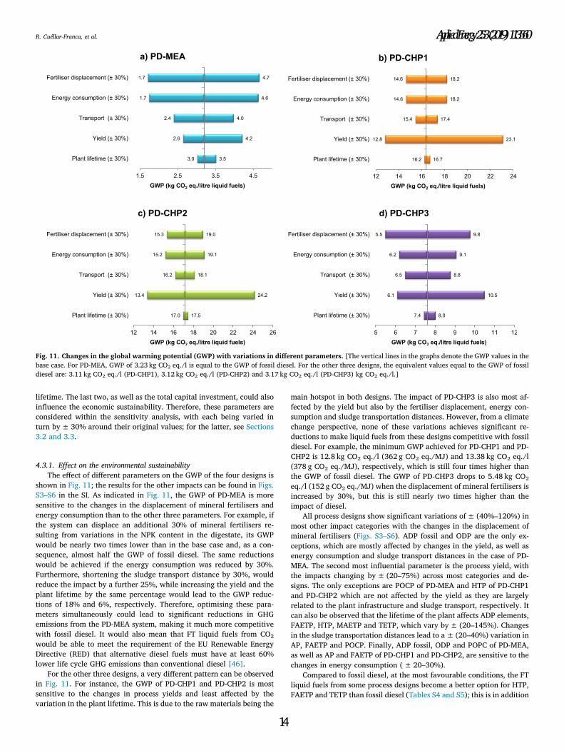
lifetime. The last two, as well as the total capital investment, could alsoinfluence the economic sustainability. Therefore, these parameters areconsidered within the sensitivity analysis, with each being varied inturn by ± 30% around their original values; for the latter, see Sections3.2 and 3.3.

4.3.1. Effect on the environmental sustainabilityThe effect of different parameters on the GWP of the four designs is

shown in Fig. 11; the results for the other impacts can be found in Figs.S3–S6 in the SI. As indicated in Fig. 11, the GWP of PD-MEA is moresensitive to the changes in the displacement of mineral fertilisers andenergy consumption than to the other three parameters. For example, ifthe system can displace an additional 30% of mineral fertilisers re-sulting from variations in the NPK content in the digestate, its GWPwould be nearly two times lower than in the base case and, as a con-sequence, almost half the GWP of fossil diesel. The same reductionswould be achieved if the energy consumption was reduced by 30%.Furthermore, shortening the sludge transport distance by 30%, wouldreduce the impact by a further 25%, while increasing the yield and theplant lifetime by the same percentage would lead to the GWP reduc-tions of 18% and 6%, respectively. Therefore, optimising these para-meters simultaneously could lead to significant reductions in GHGemissions from the PD-MEA system, making it much more competitivewith fossil diesel. It would also mean that FT liquid fuels from CO2

would be able to meet the requirement of the EU Renewable EnergyDirective (RED) that alternative diesel fuels must have at least 60%lower life cycle GHG emissions than conventional diesel [46].

For the other three designs, a very different pattern can be observedin Fig. 11. For instance, the GWP of PD-CHP1 and PD-CHP2 is mostsensitive to the changes in process yields and least affected by thevariation in the plant lifetime. This is due to the raw materials being the

main hotspot in both designs. The impact of PD-CHP3 is also most af-fected by the yield but also by the fertiliser displacement, energy con-sumption and sludge transportation distances. However, from a climatechange perspective, none of these variations achieves significant re-ductions to make liquid fuels from these designs competitive with fossildiesel. For example, the minimum GWP achieved for PD-CHP1 and PD-CHP2 is 12.8 kg CO2 eq./l (362 g CO2 eq./MJ) and 13.38 kg CO2 eq./l(378 g CO2 eq./MJ), respectively, which is still four times higher thanthe GWP of fossil diesel. The GWP of PD-CHP3 drops to 5.48 kg CO2

eq./l (152 g CO2 eq./MJ) when the displacement of mineral fertilisers isincreased by 30%, but this is still nearly two times higher than theimpact of diesel.

All process designs show significant variations of ± (40%–120%) inmost other impact categories with the changes in the displacement ofmineral fertilisers (Figs. S3–S6). ADP fossil and ODP are the only ex-ceptions, which are mostly affected by changes in the yield, as well asenergy consumption and sludge transport distances in the case of PD-MEA. The second most influential parameter is the process yield, withthe impacts changing by ± (20–75%) across most categories and de-signs. The only exceptions are POCP of PD-MEA and HTP of PD-CHP1and PD-CHP2 which are not affected by the yield as they are largelyrelated to the plant infrastructure and sludge transport, respectively. Itcan also be observed that the lifetime of the plant affects ADP elements,FAETP, HTP, MAETP and TETP, which vary by ± (20–145%). Changesin the sludge transportation distances lead to a ± (20–40%) variation inAP, FAETP and POCP. Finally, ADP fossil, ODP and POPC of PD-MEA,as well as AP and FAETP of PD-CHP1 and PD-CHP2, are sensitive to thechanges in energy consumption ( ± 20–30%).

Compared to fossil diesel, at the most favourable conditions, the FTliquid fuels from some process designs become a better option for HTP,FAETP and TETP than fossil diesel (Tables S4 and S5); this is in addition

Fig. 11. Changes in the global warming potential (GWP) with variations in different parameters. [The vertical lines in the graphs denote the GWP values in thebase case. For PD-MEA, GWP of 3.23 kg CO2 eq./l is equal to the GWP of fossil diesel. For the other three designs, the equivalent values equal to the GWP of fossildiesel are: 3.11 kg CO2 eq./l (PD-CHP1), 3.12 kg CO2 eq./l (PD-CHP2) and 3.17 kg CO2 eq./l (PD-CHP3) kg CO2 eq./l.]


14

to the other five impacts for which they were better in the base case(Fig. 9). For example, increasing the displacement of mineral fertilisersby 30% reduces the HTP of PD-MEA and PD-CHP3 by 31% and 36%relative to diesel and TETP by 18% and 32%, respectively. In addition,FAETP of all process designs is also reduced significantly on the basecase, with PD-CHP3 becoming net-negative for this impact and a betteroption than fossil diesel. However, ADP elements and ODP still remainhigher across the designs than the equivalent impacts of diesel. Even byextending the plant lifetime by 30%, the ADP elements is still 16–36times higher than for diesel. Finally, ODP remains 25–30% higher thanthat of diesel for the best values of any of the parameters considered.

4.3.2. Effect on the economic sustainabilityThe effect of the plant lifetime on the LCC and profitability of the

different designs is shown in Fig. 10. Increasing the lifetime from 20 to26 years, increases the LCC by 24%, while reducing it to 14 years lowersthe costs by 24% across the designs. It can also be observed that the LCCof PD-MEA over 26 years are comparable to the CHP-based plants iftheir lifetime is kept at 20 years. This would also lead to a competitiveprofitability of this process compared to the rest whilst maintaininglower fuel prices. For example, for a MARR of 8%, PD-CHP1 would earna profit of £70 million over 20 years at a basic price of fuel of 3,645pence per litre. By comparison, PD-MEA would gain £71 million over26 years for a price of fuel of 2,466 pence per litre.

The basic fuel price would also be reduced with an increase in theyield and a reduction in TCI. For a MARR of 8%, increasing the yield by30% would decrease the fuel price across the designs by 23% (Fig. 12).However, if the yield was 30% lower than in the base case, the fuelprice would increase by 43%. Increasing the TCI by 30% would increasethe basic prices by 20–30% while reducing the TCI by 30% would de-crease them by 33% across the designs. Similar trends are found for theother MARR values (Figs. S7–S9 in the SI). However, under the bestconditions, these prices would still be much higher than the price offossil diesel. As mentioned earlier, this is largely due to the small-scaleproduction considered so far. The issue of scale is explored further inthe next section.

4.4. Plant scale-up

This section examines the effect of the economies of scale on theenvironmental and economic sustainability of the four process designsconsidered in the previous sections. Two production capacities areconsidered: medium and large, producing 850 and 1,670 tonnes of li-quid fuels per day, respectively. The scaling-up has been carried outfollowing the methodology explained in Section 3.3.5.

4.4.1. Life cycle environmental sustainabilityOnly the impacts of the large-scale plants are discussed here as the

trends are similar to the medium scale. The results for the latter can befound in Figs. S10 and S11 in the SI.

As shown in Fig. 13, the FT fuels from the scaled-up plants out-perform fossil diesel in all impact categories across all the designs. Theonly exceptions are the ODP, for which fossil diesel is the best option,and the GWP, which is lower for fossil diesel than for the CHP-baseddesigns. However, PD-MEA now has a 24% lower GWP than fossil dieseland is the best option from a climate change perspective. Nevertheless,it still has a higher impact than the 1st or 2nd generation biofuels. Forthe other impacts, PD-CHP3 now emerges as the most sustainable al-ternative among the four designs, except for ADP fossil and POCP,where the MEA design is better and, as previously mentioned, ODP forwhich fossil diesel is preferred.

It is notable that, with the scaling-up, ADP elements, FAETP, HTP andTETP improve substantially and become net-negative. This is due to amuch lower requirements for the plant infrastructure per unit of FT fuelsproduced. For that reason, the reduction in ADP elements is particularlysignificant – from being 35–50 times higher than that of fossil diesel in thebase case (Fig. 9), it is now around 25–50 times lower (Fig. 13). Thechange in the remaining impacts (ADP fossil, AP, EP, MAETP, ODP andPOCP) with the scaling-up is negligible. The reason for this is that thecontribution of the plant infrastructure to these impacts is minimal, bothin the base case (Fig. 7) and scaled-up plants (Fig. S12). However, aslarger plants are typically more resource efficient, it is likely that all theseand the remaining impacts would improve further. In the absence of realdata, it is not possible to consider fully the effect of the economies of scaleon the resource consumption and the related reductions in impacts. In-stead, this is explored in a sensitivity analysis, focusing on PD-MEA,which outperforms fossil diesel for all impacts but ODP.

Varying the same parameters as in the base-case sensitivity analysis(Section 4.3.1) by ± 30% would change the GWP of the scaled-up PD-MEA as shown in Fig. 14; the effect on the other impacts can be seen inFig. S13 in the SI. As in the base case, the amount of mineral fertilisersdisplaced and the process energy consumption have the greatest effecton the GWP. In the best case, the GWP reduces to 1 kg CO2 eq./l or 27 gCO2 eq./MJ, which is around 70% lower than the impact of fossil diesel.However, in the worst case, the GWP of FT liquid fuels increases to3.95 kg CO2 eq./l (107 g CO2 eq./MJ), 18% higher than for fossil diesel.Decreasing sewage transport distances and increasing the yield by 30%each reduces the impact to 1.68 and 1.92 kg CO2 eq./l, which is 50%and 40% lower than for fossil diesel, respectively. The equivalentchanges in the opposite direction lead to a 1–8% higher impact thanthat of diesel. The GWP is unaffected by the changes in the plant life-time as the infrastructure plays a much smaller role in this impact forlarge plants.

Fig. 12. Changes in the basic fuel price with the total capital investment (TCI) and production yield for a minimum acceptable rate of return of 8%. [Thevertical lines in the graphs represent the basic price in the base case.]


15

The above results for can be used to estimate the potential for mi-tigating the climate change impact from the transport sector by dis-placing a certain share of fossil diesel with FT liquid fuels. In 2017,30.4 billion tonnes of diesel were consumed in the UK [47], emitting95 Mt CO2 eq. of GHG emissions [48]. The revised Renewable TransportFuels Obligation (RTFO) stipulates through the fuel blending obligationthat 9.75% of fossil fuels should be replaced by alternative fuels by2020 and 12.4% by 2032 [49]. Assuming hypothetically that all of thisreplacement is met through CO2-derived fuels from large-scale PD-MEAplants, gives the maximum GHG mitigation potentials in Fig. 15. Thishas been calculated considering the base-case and the improved GWPvalues shown in Fig. 14, assuming that the actual plants will be opti-mised and hence their impacts reduced rather than increased. In thatcase, FT liquid fuels could avoid around 2–8 Mt CO2 eq. annually bydisplacing fossil diesel, with 2 and 2.5 Mt CO2 eq. avoided in the basecase for the displacements of 9.75% and 12.4% of fossil diesel, re-spectively. Therefore, there is a clear potential for FT fuels produced inlarge-scale PD-MEA plants to contribute towards mitigation of the cli-mate change impact from transport. This would also lead to reductionsin all other life cycle impacts considered here, ranging from 8% and13% for POCP and ADP fossil to 170–480% for MAETP and ADP ele-ments for the displacement of 9.75% and 12.4% of fossil diesel, re-spectively. The only exception is ODP which would increase by 7% and8% (Table S6).

Their economic potential at large-scale production is explored next.

4.4.2. Life cycle economic sustainabilityThe life cycle costs and profits of the scaled-up process designs are

presented in Fig. 16 for a MARR of 8%; the profit values for the otherMARRs can be found in Fig. S13 in the SI. As can be seen in Fig. 16, theLCC for the medium-size plants are 80–100 times higher than in thebase case, while the larger plants have 130–160 times greater costs,depending on the design. However, the larger plants are more profit-able due to the economies of scale. In the worst case, a medium-scalePD-MEA would earn around £3.7 billion in profits over 20 years, whilein the best case, large-scale PD-CHP3 would have a profit of around£8.4 billion.

Fig. 13. Life cycle environmental impacts of Fischer-Tropsch fuels produced from CO2 in a large-scale plant (1,670 t/day) in comparison with fossil diesel.[The values for some impacts have been scaled to fit. The original values can be obtained by multiplying the value shown on top/bottom of the bars by the scalingfactor given on the x-axis. GWP data for fossil diesel sourced from: Azapagic and Stichnothe [43], Defra [44], Jeswani and Azapagic [45], and Ecoinvent Centre [27];data for other environmental impacts sourced from Ecoinvent [27]. See Fig. 7 for impacts acronyms.]

Fig. 14. Changes in the global warming potential (GWP) for PD-MEA withvariations in different parameters for a large-scale plant (1,670 t/day).[The vertical lines in the graphs denote the original GWP value (2.47 kg CO2

eq./l). GWP of 3.23 kg CO2 eq./l is equal to the GWP of fossil diesel.]

Fig. 15. Global warming potential (GWP) potentially avoided by displa-cing fossil diesel based on the Renewable Transport Fuels Obligation(RTFO). [Values shown for PD-MEA. Based on consumption of fossil diesel inthe UK in 2017, sourced from BEIS [48] and RAC [47]. RTFO: RenewableTransport Fuels Obligation [49].]


16

Both the costs and profits are affected by the plant lifetime. Forexample, extending the lifetime of the PD-MEA from 20 to 26 yearswould increase its profits by 8% while decreasing it to 14 years wouldlead to 8% lower net earnings (Fig. 16).

Based on the profitability analysis of the scaled-up plants, the esti-mated basic prices of FT fuels decrease considerably with the increasein capacity (Fig. 17). For the large-scale plant (1,670 t/day), PD-MEAhas the lowest basic price of 185 pence/l at 8% MARR, increasing to300 pence/l for the MARR of 24%. Thus, even in the best case, this isstill four times higher than the basic price of fossil diesel consideredhere (44.4 pence/l). However, it should be noted that a biodiesel wasalso significantly more expensive than fossil diesel a few years ago. Forexample, in 2013, their respective wholesale prices in the EU were€0.85 and €0.47/l [50] but the gap has closed since due to a widerdeployment of biodiesel, as mandated by the RED, and the increasingprices of diesel.

The basic prices for the other three designs range from 221 to275 pence/l for 8% MARR and 357–447 pence/l for the MARR of 24%.Thus, in the worst case for the large plant (PD-CHP3 @ 24% MARR), FTfuels are ten times more expensive than fossil diesel. For the medium-scale capacity, the basic prices range from 226 to 561 pence/l across thedesigns and MARRs; this is 5–13 times greater than the price of diesel.

These prices are also unfavourable in comparison to other FT liquidfuels reported in the literature. For example, the basic price of FT dieselproduced from natural gas ranges from 9 to 47 pence/l [7]. For coal-derived diesel, it is 30 pence/l [7] and around 56 pence for fuels pro-duced in a CBTL plant [10]. However, CO2-derived FT fuels comparemore favourably with the basic price of algae biodiesel, which can be ashigh as 2,300 pence/l depending on estimates [51].

Assuming the same taxation for CO2-derived FT fuels as for theconventional road fuels, with 63% of the pump price being the exciseduty and VAT, the pump prices of these fuels would range from 500

Fig. 16. Life cycle costs (top) and profits @ 8% MARR (bottom) for different designs and production capacities. [Base case: > 1 t/day; Medium scale: 850 t/day; Large scale: 1,670 t/day. The values shown on top of graph bar refer to the plant lifetime of 20 years while the lower and upper error bars correspond to the costsfor the lifetime of 14 and 26 years, respectively.]


17

pence (large-scale PD-MEA @ 8% MARR) to 1,516 pence (medium-scalePD-CHP3 @ 24% MARR), compared to the assumed 120 pence for alitre of fossil diesel (Table 14). Therefore, these fuels would not be vi-able without either reducing the taxation, providing subsidies and/ormandating their use through policy. Similar applies to biofuels, whichare still not economically viable and would not be produced withoutstrong policy incentives [52]. In addition to the fuel blending obligationmandated through the RTFO, this also included a 20 pence/l exciseduty exemption until 2012.

The issue of taxation and incentives is considered in Fig. 18, whichshows that subsidies would be required in all cases, ranging from 35%to 79% of the pump price of 120 pence/l, depending on the processdesign, production scale and the MARR.

The tax margins and subsidies are explored further through a sen-sitivity analysis by varying the TCI and production yields by ± 30%.The results in Fig. 19 suggest that in the best case, subsidies could bereduced to 8% but in the worst case, they would need to be at the levelof 70–85%.

0

200

400

600

800

1000

1200

1400

1600

1800

2000

2200

2400

2600

0 200 400 600 800 1000 1200 1400 1600 1800

Basic price (pence per litre)

a) PD-MEA

MARR 8%

MARR 16%

MARR 20%

MARR 24%

0

200

400

600

800

1000

1200

1400

1600

1800

2000

2200

2400

2600

0 200 400 600 800 1000 1200 1400 1600 1800


b) PD-CHP1

MARR 8%

MARR 16%

MARR 20%

MARR 24%

0

200

400

600

800

1000

1200

1400

1600

1800

2000

2200

2400

2600

0 200 400 600 800 1000 1200 1400 1600 1800


Plant capacity (t/day)


c) PD-CHP2

MARR 8%

MARR 16%

MARR 20%

MARR 24%

0

200

400

600

800

1000

1200

1400

1600

1800

2000

2200

2400

2600

0 200 400 600 800 1000 1200 1400 1600 1800




d) PD-CHP3

MARR 8%

MARR 16%

MARR 20%

MARR 24%

Fig. 17. Estimated basic price (excluding excise duty and VAT) of Fischer-Tropsch liquid fuels for different plant capacities. [The y-axis has been capped at2,600 pence/l to enable a better comparison between process designs. The basic prices for small (base-case) capacity can be found in Table 13.]

Table 14Hypothetical price at pump of Fischer-Tropsch liquid fuels for different plant capacities considering the same road taxation as for fossil diesel (pence per litre).

Price/tax PD-MEA PD-CHP1 PD-CHP2 PD-CHP3

8% 16% 20% 24% 8% 16% 20% 24% 8% 16% 20% 24% 8% 16% 20% 24%

Medium-scale plant (850 t/day)Basic price 226 301 339 376 269 358 403 447 284 379 427 474 336 449 505 561Excise duty and VATa 385 513 577 641 458 610 686 762 483 645 726 807 572 764 860 955Price at pump 610 814 915 1,017 728 968 1,089 1,209 767 1,024 1,153 1,282 908 1,212 1,364 1,516

Large-scale plant (1670 t/day)Basic price 185 243 271 300 221 289 323 357 232 305 341 378 275 361 404 447Excise duty and VATa 315 413 462 511 376 492 550 608 396 519 581 643 469 615 688 761Price at pump 500 656 733 811 597 781 873 965 628 824 922 1,021 744 976 1,092 1,208

a 63% of the total pump price.

Fig. 18. Subsidies required for Fischer-Tropsch liquid fuels to match fossildiesel pump prices. [Based on the range of basic prices for the medium (850 t/day) and large (1,670 t/day) plant capacities for different process designs andMARRs as shown in Fig. 17.]


18

5. Conclusions

This paper has evaluated the life cycle environmental and economicsustainability of FT liquid fuels produced from CO2 generated duringanaerobic digestion of sewage sludge. Four process configurations havebeen considered and the sustainability evaluated for a range of plantcapacities to explore the effect of the economies of scale. For a smallscale production (< 1 t fuels/day), the lowest global warming potential(GWP) of 87 g CO2 eq./MJ estimated for PD-MEA matches the GWP offossil diesel. However, the highest impact of 484 g CO2 eq./MJ (PD-CHP2) is 5.5 times higher than that of diesel. Liquid fuels from PD-MEAalso have the lowest other environmental impacts compared to the fuelsfrom the other three designs. In comparison with diesel, PD-MEA fuelsare better for five impact categories while diesel is environmentallymore sustainable for the remaining five impacts.

The results suggest that PD-MEA is the least costly but PD-CHP3 isthe most profitable design. However, the latter has the highest esti-mated basic price, ranging from 4,736 to 8,609 pence per litre, de-pending on the MARR. The lowest fuel prices of 2,601–4,808 pence/lare found for PD-MEA. These are 60–190 times higher than the averagebasic price of fossil diesel in 2017 of 44.4 pence per litre.

Both the environmental and economic sustainability improve sig-nificantly with the economies of scale. For the large-scale plants(1,670 t/day), the FT fuels outperform fossil diesel in all impacts acrossall the designs, with several impacts being net-negative. The only ex-ceptions are the ODP, for which fossil diesel is still the best option, andthe GWP, which is lower for fossil diesel than for the CHP-based de-signs. Optimising the key parameters for the scaled-up plants leads tothe GWP of FT fuels from PD-MEA being up to 70% lower than that ofdiesel. Therefore, FT fuels from CO2 have a potential to reduce GHGemissions from the transport sector. Following the RTFO fuel blendingobligation, and assuming a hypothetical replacement of 9.75–12.4% ofdiesel by FT fuels from CO2, would mitigate 2–8 Mt of CO2 eq./yr,equivalent to around 2–8% of emissions from the transport sector.

The fuel prices are also significantly lower for the large plants,

reducing to 185 pence per litre in the best case (PD-MEA at 8% MARR),but this is still four times higher than the price of diesel. Thus, thesefuels would not be economically viable without either reducing thetaxation, providing subsidies and/or mandating their use throughpolicy, in a similar manner the biofuels markets have been stimulated.The results obtained in this work suggest that matching the diesel pumpprice of 120 pence/litre would require subsidies between 35% and 79%,depending on the MARR and the scale of production. If the productionyields can be improved by 30%, subsidies could be reduced to 8%.

While the economies of scale and policy will help to improve thecompetitiveness of these fuels, further technological developments arealso essential to optimise key process parameters. These include moreefficient CO2 capture and conversion processes as well as novel sorbentsand catalysts aimed at reducing energy consumption and increasingfuel production yields. Future research should also explore differentpolicy mechanisms for stimulating development of the markets for CO2-derived fuels.

Acknowledgements

This work was carried out as part of the “4CU” Programme Grant,aimed at sustainable conversion of carbon dioxide into fuels, led by TheUniversity of Sheffield and carried out in collaboration with TheUniversity of Manchester, Queens University Belfast and UniversityCollege London. The authors acknowledge gratefully the UKEngineering and Physical Sciences Research Council (EPSRC) for sup-porting this work financially (Grant No. EP/K001329/1). Thanks toNathalie Gaytan Franca for the artwork for the graphical abstract.

Appendix A. Supplementary material

Supplementary data to this article can be found online at https://doi.org/10.1016/j.apenergy.2019.113560.

Fig. 19. Effect of the total capital investment (TCI) and production yield on subsidies and taxation. [Based on the range of basic prices for the medium (850 t/d) and large (1,670 t/d) plant capacities for different process designs and MARRs as shown in Fig. 17.]


19



References

[1] USCC. International index of energy security risk: assessing risk in a global energymarket. U.S. Chamber of Commerce's Institute for 21st Century Energy; 2015.< http://www.energyxxi.org/sites/default/files/pdf/energyrisk_intl_2015.pdf > .

[2] Styring P, Jansen D, de Coninck H, Reith H, Armstrong K. Carbon capture andutilisation in the green economy. Centre for Low Carbon Futures; 2011. < http://co2chem.co.uk/wp-content/uploads/2012/06/CCU%20in%20the%20green%20economy%20report.pdf > .

[3] Assen NVD, Sternberg A, Katelhon A, Bardow A. Environmental potential of carbondioxide utilization in the polyurethane supply chain. Faraday Discuss2015;183:291–307.

[4] Olivier JGJ, Schure KM, Peters JAHW. Trends in global CO2 and total greenhousegas emissions. PBL Netherlands Environmental Assessment Agency; 2017.< https://www.pbl.nl/sites/default/files/cms/publicaties/pbl-2017-trends-in-global-co2-and-total-greenhouse-gas-emissons-2017-report_2674.pdf > .

[5] Dimitriou I, Garcia-Gutierrez P, Elder RH, Cuellar-Franca RM, Azapagic A, AllenRWK. Carbon dioxide utilisation for production of transport fuels: process andeconomic analysis. Energy Environ Sci 2015;8(6):1775–89.

[6] Dry ME. High quality diesel via the Fischer-Tropsch process – a review. J ChemTechnol Biotechnol 2002;77(1):43–50.

[7] Jaramillo P, Griffin WM, Matthews HS. Comparative analysis of the productioncosts and life-cycle GHG emissions of FT liquid fuels from coal and natural gas.Environ Sci Technol 2008;42(20):7559–65.

[8] Cao Y, Gao Z, Jin J, Zhou H, Cohron M, Zhao H, et al. Synthesis gas production withan adjustable H2/CO ratio through the coal gasification process: effects of coalranks and methane addition. Energy Fuels 2008;22(3):1720–30.

[9] Lauven L-P. Optimization of biomass-to-liquid plant setups and capacity usingnonlinear programming. Ph.D thesis. Georg-August-Universität Göttingen; 2011.

[10] Liu W, Wang J, Bhattacharyya D, Jiang Y, DeVallance D. Economic and environ-mental analyses of coal and biomass to liquid fuels. Energy 2017;141:76–86.

[11] Ahmadi Moghaddam E, Ahlgren S, Hulteberg C, Nordberg Å. Energy balance andglobal warming potential of biogas-based fuels from a life cycle perspective. FuelProcess Technol 2015;132:74–82.

[12] Wang B, Gebreslassie BH, You F. Sustainable design and synthesis of hydrocarbonbiorefinery via gasification pathway: Integrated life cycle assessment and tech-noeconomic analysis with multiobjective superstructure optimization. ComputChem Eng 2013;52:55–76.

[13] Graves C, Ebbesen SD, Mogensen M, Lackner KS. Sustainable hydrocarbon fuels byrecycling CO2 and H2O with renewable or nuclear energy. Renew Sustain EnergyRev 2011;15(1):1–23.

[14] Brynolf S, Taljegard M, Grahn M, Hansson J. Electrofuels for the transport sector: areview of production costs. Renew Sustain Energy Rev 2018;81:1887–905.

[15] Abanades JC, Rubin ES, Mazzotti M, Herzog HJ. On the climate change mitigationpotential of CO2 conversion to fuels. Energy Environ Sci 2017;10(12):2491–9.

[16] Deutz S, Bongartz D, Heuser B, Kätelhön A, Schulze Langenhorst L, Omari A, et al.Cleaner production of cleaner fuels: wind-to-wheel – environmental assessment ofCO2-based oxymethylene ether as a drop-in fuel. Energy Environ Sci2018;11(2):331–43.

[17] Hombach LE, Doré L, Heidgen K, Maas H, Wallington TJ, Walther G. Economic andenvironmental assessment of current (2015) and future (2030) use of E-fuels inlight-duty vehicles in Germany. J Cleaner Prod 2019;207:153–62.

[18] van der Giesen C, Kleijn R, Kramer GJ. Energy and climate impacts of producingsynthetic hydrocarbon fuels from CO2. Environ Sci Technol 2014;48(12):7111–21.

[19] Tsongidis NI, Asimakopoulou AG, Pantoleontos G, Konstandopoulos AG.Transportation and solar-aided utilization of CO2: technoeconomic analysis ofspanning routes of CO2 conversion to solar fuels. J CO2 Util 2019;30:142–57.

[20] Badgett A, Newes E, Milbrandt A. Economic analysis of wet waste-to-energy re-sources in the United States. Energy 2019;176:224–34.

[21] Hernandez B, Martin M. Optimization for biogas to chemicals via tri-reforming.Analysis of Fischer-Tropsch fuels from biogas. Energy Convers Manage2018;174:998–1013.

[22] Pressley PN, Aziz TN, DeCarolis JF, Barlaz MA, He F, Li F, et al. Municipal solidwaste conversion to transportation fuels: a life-cycle estimation of global warmingpotential and energy consumption. J Cleaner Prod 2014;70:145–53.

[23] Petersen AM, Melamu R, Knoetze JH, Görgens JF. Comparison of second-generationprocesses for the conversion of sugarcane bagasse to liquid biofuels in terms ofenergy efficiency, pinch point analysis and Life Cycle Analysis. Energy ConversManage 2015;91:292–301.

[24] AspenTechnology. Aspen Plus Version 8.4. Burlington, MA, USA; 2013.[25] Muleja AA, Yao Y, Glasser D, Hildebrandt D. Effect of feeding nitrogen to a fixed

bed Fischer-Tropsch reactor while keeping the partial pressures of reactants the

same. Chem Eng J 2016;293:151–60.[26] Savost’yanov AP, Yakovenko RE, Narochnyi GB, Lapidus AL. Effect of the dilution of

synthesis gas with nitrogen on the Fischer-Tropsch process for the production ofhydrocarbons. Solid Fuel Chem 2015;49(6):356–9.

[27] Ecoinvent. Ecoinvent database 2.1. Ecoinvent Centre; 2013. < http://www.ecoinvent.org/home.html > .

[28] IEA. Hydrogen production & distribution. IEA Energy Technology Essentials; 2007.< http://www.iea.org/techno/essentials5.pdf > .

[29] BEIS. Energy trends March 2018. Department for Business, Energy & IndustrialStrategy; 2018b. < www.gov.uk/government/statistics/energytrends-march-2018 > .

[30] ISO. ISO 14067 – greenhouse gases – carbon footprint of products – requirementsand guidelines for quantification and communication; 2013. < https://bsol.bsigroup.com/Bibliographic/BibliographicInfoData/000000000030244913 > .

[31] Peters MS, Timmerhaus KD, West RE. Plant design and economics for chemicalengineers, 5th ed. McGraw-Hill; 2004.

[32] Bolton P. Petrol and diesel prices. House of Commons Library; 2018. < https://researchbriefings.parliament.uk/ResearchBriefing/Summary/SN04712 > .

[33] NCS. Large goods vehicle driver job profile. National Careers Service; 2015.[34] Cebr. The CEBR-FSB employment costs index. Centre for Economics and Business

Research; 2014. < http://www.cebr.com/wp-content/uploads/2014/10/Small-Business-Employment-Costs-August-FINAL.pdf > .

[35] Seeley A. Taxation of road fuels. House of Commons Library; 2018. < https://researchbriefings.parliament.uk/ResearchBriefing/Summary/SN00824 > .

[36] Remer DS, Nieto AP. A compendium and comparison of 25 project evaluationtechniques. Part 2: Ratio, payback, and accounting methods. Int J Prod Econ1995;42(2):101–29.

[37] Hicks DI, Crittenden BD, Warhurst AC. Design for decommissioning: addressing thefuture closure of chemical sites in the design of new plant. Process Saf Environ Prot2000;78(6):465–79.

[38] Sinnott RK. Coulson & Richardson's chemical engineering: chemical engineeringdesign, 3rd ed., vol. 6. Butterworth-Heinemann; 1999.

[39] Eilers J, Posthuma SA, Sie ST. The shell middle distillate synthesis process (SMDS).Catal Lett 1990;7(1):253–69.

[40] Thinkstep. Gabi V6.4. Thinkstep; 2014. < https://www.thinkstep.com/software/gabi-lca/ > .

[41] Guinée JB, Gorrée M, Heijungs R, Huppes G, Kleijn R, de Koning A. Life cycle as-sessment: an operational guide to the ISO standards; 2001. < http://media.leidenuniv.nl/legacy/new-dutch-lca-guide-part-1.pdf > .

[42] Lipman T, Delucchi M. Emissions of nitrous oxide and methane from conventionaland alternative fuel motor vehicles. Clim Change 2002;53(4):477–516.

[43] Azapagic A, Stichnothe H. Sustainability assessment of biofuels. 2nd ed. SustainableDevelopment in Practice: Case Studies for Engineers and Scientists; 2011.

[44] Defra. 2011 guidelines to defra/DECC’s GHG conversion factors for company re-porting, version 1.0. Department for Environmentl, Food and Rural Affairs; 2011.< http://archive.defra.gov.uk/environment/business/reporting/pdf/110707-guidelines-ghg-conversion-factors.pdf > .

[45] Jeswani H, Azapagic A. Life cycle sustainability assessment of second generationbiodiesel. In: Luque, Melero, editors. Advances in biodiesel production: processesand technologies. Woodhead Publishing; 2012.

[46] EC. Directive 2009/28/EC of the European Parliament and of the Council of 23April 2009 on the Promotion of the Use of Energy from Renewable Sources:European Commission: Brussels; 2009. < https://eur-lex.europa.eu/legal-content/EN/TXT/?uri=CELEX:32009L0028 > .

[47] RAC. UK petrol and diesel quantities consumed. Royal Automobile ClubFoundation; 2017. < https://www.racfoundation.org/data/volume-petrol-diesel-consumed-uk-over-time-by-year > .

[48] BEIS. 2017 UK greenhouse gas emissions, provisional figures. Department forBusiness, Energy & Industrial Strategy; 2018a. < https://www.gov.uk/government/collections/finaluk-greenhouse-gas-emissions-national-statistics > .

[49] DfT. The renewable transport fuels and greenhouse gas emissions regulations 2018.Department for Transport, London; 2018. < https://www.legislation.gov.uk/ukdsi/2018/9780111164242 > .

[50] Charles C, Gerasimchuk I, Bridle R, Moerenhout T, Asmelash E, Laan T. Biofuels—atwhat cost? A review of costs and benefits of EU biofuel policies. The InternationalInstitute for Sustainable Development; 2013. < https://www.agrireseau.net/energie/documents/biofuels_subsidies_eu_review.pdf > .

[51] ECOFYS. How to advance cellulosic biofuels – assessment of costs, investment op-tions and policy support: ECOFYS Consultancy; 2016.

[52] RAEng. Sustainability of biofuels. Royal Academy of Engineering. London; 2017.< https://www.raeng.org.uk/publications/reports/biofuels > .


20

http://www.energyxxi.org/sites/default/files/pdf/energyrisk_intl_2015.pdf

http://co2chem.co.uk/wp-content/uploads/2012/06/CCU%20in%20the%20green%20economy%20report.pdf



http://refhub.elsevier.com/S0306-2619(19)31234-6/h0015



https://www.pbl.nl/sites/default/files/cms/publicaties/pbl-2017-trends-in-global-co2-and-total-greenhouse-gas-emissons-2017-report_2674.pdf

https://www.pbl.nl/sites/default/files/cms/publicaties/pbl-2017-trends-in-global-co2-and-total-greenhouse-gas-emissons-2017-report_2674.pdf




























































http://www.ecoinvent.org/home.html

http://www.ecoinvent.org/home.html

http://www.iea.org/techno/essentials5.pdf

http://www.gov.uk/government/statistics/energytrends-march-2018

http://www.gov.uk/government/statistics/energytrends-march-2018

https://bsol.bsigroup.com/Bibliographic/BibliographicInfoData/000000000030244913

https://bsol.bsigroup.com/Bibliographic/BibliographicInfoData/000000000030244913

https://researchbriefings.parliament.uk/ResearchBriefing/Summary/SN04712



http://www.cebr.com/wp-content/uploads/2014/10/Small-Business-Employment-Costs-August-FINAL.pdf

http://www.cebr.com/wp-content/uploads/2014/10/Small-Business-Employment-Costs-August-FINAL.pdf











https://www.thinkstep.com/software/gabi-lca/

https://www.thinkstep.com/software/gabi-lca/

http://media.leidenuniv.nl/legacy/new-dutch-lca-guide-part-1.pdf

http://media.leidenuniv.nl/legacy/new-dutch-lca-guide-part-1.pdf





http://archive.defra.gov.uk/environment/business/reporting/pdf/110707-guidelines-ghg-conversion-factors.pdf

http://archive.defra.gov.uk/environment/business/reporting/pdf/110707-guidelines-ghg-conversion-factors.pdf

https://eur-lex.europa.eu/legal-content/EN/TXT/?uri=CELEX:32009L0028

https://eur-lex.europa.eu/legal-content/EN/TXT/?uri=CELEX:32009L0028

https://www.racfoundation.org/data/volume-petrol-diesel-consumed-uk-over-time-by-year

https://www.racfoundation.org/data/volume-petrol-diesel-consumed-uk-over-time-by-year

https://www.gov.uk/government/collections/finaluk-greenhouse-gas-emissions-national-statistics

https://www.gov.uk/government/collections/finaluk-greenhouse-gas-emissions-national-statistics

https://www.legislation.gov.uk/ukdsi/2018/9780111164242

https://www.legislation.gov.uk/ukdsi/2018/9780111164242

https://www.agrireseau.net/energie/documents/biofuels_subsidies_eu_review.pdf

https://www.agrireseau.net/energie/documents/biofuels_subsidies_eu_review.pdf

https://www.raeng.org.uk/publications/reports/biofuels

Documents

Utilising carbon dioxide for transport fuels : the