Using the Soil and Water Assessment Tool (SWAT) to ... · Using the Soil and Water Assessment Tool (SWAT) to Simulate Runoff in Mustang Creek Basin, California By Dina K. Saleh, Charles

Using the Soil and Water Assessment Tool (SWAT) to Simulate Runoff in Mustang Creek Basin, California

U.S. Department of the InteriorU.S. Geological Survey

Scientific Investigations Report 2009–5031

Cover: Horses at Mustang Ranch, California. (Photograph by Dina Saleh, U.S. Geological Survey, 2004)


By Dina K. Saleh, Charles R. Kratzer, Colleen H. Green, and David G. Evans

Scientific Investigations Report 2009–5031

U.S. Department of the InteriorU.S. Geological Survey

iii

U.S. Department of the InteriorKEN SALAZAR, Secretary

U.S. Geological SurveySuzette M. Kimball, Acting Director

U.S. Geological Survey, Reston, Virginia: 2009

For more information on the USGS—the Federal source for science about the Earth, its natural and living resources, natural hazards, and the environment, visit http://www.usgs.gov or call 1-888-ASK-USGS

For an overview of USGS information products, including maps, imagery, and publications, visit http://www.usgs.gov/pubprod

To order this and other USGS information products, visit http://store.usgs.gov

Any use of trade, product, or firm names is for descriptive purposes only and does not imply endorsement by the U.S. Government.

Although this report is in the public domain, permission must be secured from the individual copyright owners to reproduce any copyrighted materials contained within this report.

Suggested citation:Saleh, D.K., Kratzer, C.R., Green, C.H., and Evans, D.G., 2009, Using the Soil and Water Assessment Tool (SWAT) to simulate runoff in Mustang Creek Basin, California: U.S. Geological Survey Scientific Investigations Report 2009–5031, 28 p.

iv

FiguresFigure 1. Location of the study area within the Mustang Creek Basin,

California .....................................................................................................................................2Figure 2. Monthly temperature at Mustang Creek Basin, obtained from Denair

weather station .........................................................................................................................3Figure 3. Monthly precipitation from Denair weather station in Stanislaus County,

California, 1988–2005 .................................................................................................................4Figure 4. Mean monthly precipitation, Denair weather station 1984–2005, and

water year 2004 ..........................................................................................................................5Figure 5. Soil data for Mustang Creek Basin, California, showing the soil formations and

mapped soil series in the study area .....................................................................................6Figure 6. Relative depth to hardpan in the Mustang Creek Basin, California ..................................7Figure 7. Detailed agricultural land use in the upper Mustang Creek Basin, California ................8Figure 8. Precipitation and 15-minute streamflow data for Mustang Creek at

Monte Vista Avenue near Montpelier, California .................................................................9

Contents

Abstract ...........................................................................................................................................................1Introduction.....................................................................................................................................................1

Purpose and Scope .............................................................................................................................1Description of Study Area ..................................................................................................................2

Climate ..........................................................................................................................................2Physiography, Geology, and Soils .............................................................................................4Land Use ........................................................................................................................................5Hydrology and Available Streamflow Data ..............................................................................5

Soil and Water Assessment Tool (SWAT) Watershed Model .................................................................6Model History ........................................................................................................................................6Previous Applications of SWAT Watershed Model .......................................................................8

Hydrologic Studies ......................................................................................................................8Calibration Technique Studies .................................................................................................10

Comparison of SWAT with other Models ........................................................................................10Runoff Model Description .................................................................................................................11Model Data Structure and Inputs ....................................................................................................13Evaluation of Model Performance ...................................................................................................14

SWAT Model Application to Mustang Creek Basin ...............................................................................15Input Data for Mustang Creek Simulations ....................................................................................15Uncalibrated Model Results .............................................................................................................16Model Calibration................................................................................................................................19Model Validation .................................................................................................................................19

Conclusions...................................................................................................................................................25References Cited .........................................................................................................................................25

v

Figure 9. Topographic relief of Mustang Creek Basin used for sub-watershed delineation in the Soil and Water Assessment Tool (SWAT) watershed simulation .........................16

Figure 10. Sub-watershed delineation of the Mustang Creek Basin, California .............................17Figure 11. Results from an uncalibrated Soil and Water Assessment Tool (SWAT)

model run for Mustang Creek Basin, California, for February 2004 ................................18Figure 12. Distribution of the curve number assigned after calibration to

sub-watersheds in the study area ........................................................................................20Figure 13. Changes in the streamflow curve due to changes in the Soil Conservation

Service curve number CN value ...........................................................................................21Figure 14. February 2004 streamflow for Mustang Creek Soil and Water Assessment Tool

(SWAT) 2005 calibration simulation results .........................................................................22Figure 15. Simulated streamflow for Mustang Creek using Soil and Water Assessment

Tool (SWAT) 2005 validation results for January and February 2005 ..............................24

TablesTable 1. Names, description, and type of data available for sites in the

Mustang Creek Basin, California ..............................................................................................3Table 2. The main soils series and formations present in the

Mustang Creek Basin, California ............................................................................................17Table 3. Statistics from the SWAT2005 uncalibrated simulation run for streamflow in

Mustang Creek, California ........................................................................................................18Table 4. Description and distribution of Soil Conservation Service curve number

assigned to the Mustang Creek Basin, California ................................................................20Table 5. Statistic results for Soil Conservation Service curve number sensitivity analysis ........21Table 6. Calibrated values of adjusted parameters for discharge calibration of the

SWAT2005 model .......................................................................................................................21Table 7. The annual hydrologic budget of the Mustang Creek Basin, California, using

SWAT2005 simulations with and without the hardpan layer ..............................................22Table 8. Statistics for calibrated simulation of streamflow in Mustang Creek, California ..........23Table 9. Statistics for validation simulation of streamflow in Mustang Creek, California ...........24

vi

Conversion Factors

Inch/Pound to SI

Multiply By To obtain

Length

inch (in.) 25.4 millimeter (mm)

foot (ft) 0.3048 meter (m)

mile (mi) 1.609 kilometer (km)

Area

acre 4,047 square meter (m2)

square mile (mi2) 259.0 hectare (ha)

Volume

cubic foot (ft3) 28.32 cubic decimeter (dm3)

acre-foot (acre-ft) 0.001233 cubic hectometer (hm3)

Flow rate

cubic foot per second (ft3/s) 0.02832 cubic meter per second (m3/s)

Temperature can be converted between degrees Celsius (°C) and degrees Fahrenheit (°F) by the formulas:

°F=(1.8×°C)+32 and °C=(°F-32)/1.8

Vertical coordinate information is referenced to the North American Vertical Datum of 1988 (NAVD 88).

vii

AbbreviationsAVSWAT ArcView extension in SWAT CN Curve NumberDEM Digital Elevation Model DataDWSM Dynamic Watershed Simulation Model ET evapotranspiration GIS Geographic Information System HRUs Hydrologic Response Units HSPF Hydrological Simulation Program–FORTRAN HYMO Hydrologic Model MID Modesto Irrigation District NSE Nash-Sutcliffe model efficiency coefficient NAWQA National Water-Quality AssessmentNED National Elevation Dataset NLCD National Land-Cover Data NOAA National Oceanic and Atmospheric Administration NRCS U.S. Natural Resource Conservation Service SCS Soil Conservation Service SD standard deviation SEA SSURGO Extension in AVSWAT SSURGO Soil Survey Geographic SWAT Soil and Water Assessment Tool SWRRB Simulator for Water Resources in Rural Basins USDS–ARS U.S. Department of Agriculture, Agricultural Research Service USGS U.S. Geological Survey

AbstractThis study is an evaluation of the calibration and valida-

tion of the Soil and Water Assessment Tool (SWAT) version 2005 watershed model for the Mustang Creek Basin, San Joa-quin Valley, California. The study is part of a national study on the process of agricultural chemical movement through the hydrologic system, which is being done by the U.S. Geologi-cal Survey (USGS) National Water-Quality Assessment pro-gram. The SWAT model was used to simulate streamflow in the Mustang Creek Basin on the basis of a set of model inputs derived and modified from various data sources.

The 2005 version of the model was calibrated for 29 days in February 2004, and validated for 58 days in January and February 2005. Measured streamflow for a USGS gaging station was used for model calibration and validation. Results of the simulated monthly streamflow had a Nash Sutcliffe effi-ciency value of 0.72 during the calibration period. The 2005 version of the model was unsuccessful in simulating stream-flow during the validation period, as indicated by a Nash Sutcliffe efficiency value of 0.33. This lack of a successful simulation probably is due to the limited amount of measured streamflow data available for calibration, the ephemeral nature of flows in Mustang Creek, and the fact that the SWAT model was developed primarily for long time periods (2 years and more) simulations and not for limited monthly simulations as used in Mustang Creek Basin.

IntroductionThe U.S. Geological Survey (USGS) started a national

study of the transport of agricultural chemicals in 2002 (Agricultural Chemicals: Sources, Transport, and Fate; ACT) as part of its National Water-Quality Assessment (NAWQA) program. The objective of that study was to understand the effect of environmental processes and agricultural practices on the transport and fate of selected nutrients and pesticides

in the hydrologic systems of nationally important agricultural settings (http://in.water.usgs.gov/NAWQA_ACT/). The national study focused on five study sites located in varied agricul-tural and hydrologic settings across the nation (in Maryland, Indiana, Nebraska, Washington, and California). One of these study sites is the Mustang Creek Basin, located in the San Joaquin Valley in central California. The Mustang Creek Basin was selected by the USGS because it is a small agricultural watershed within the Merced River Basin that has been moni-tored by NAWQA since 1993 (Gronberg and Kratzer, 2006). The San Joaquin Valley is one of the most productive agricul-tural areas in the world (Gronberg and Kratzer, 2006). Many fertilizers, such as manure, urea, and anhydrous ammonia, and pesticides are applied to the great diversity of crops grown in the valley. Relatively high concentrations of nitrate and pesticides have been found in the San Joaquin River (Panshin and others, 1998; and Kratzer and others, 2004). Therefore, it is important to understand the relation between the application of fertilizers and pesticides in the valley and the concentra-tion of nutrients and pesticides in the surface water therein. One way to assess the relation between nutrient and pesticide application in agricultural areas and resultant nutrient and pesticide concentrations in streamflow is to use a watershed model capable of simulating streamflow and chemical trans-port. Because of its widespread use in the agricultural research community, the U.S. Department of Agriculture (USDA) Soil and Water Assessment Tool (SWAT) was chosen by ACT as the watershed model to apply to each of the five study areas (Neitsch and others, 2005; Capel and others, 2008).

Purpose and Scope

The objective of this study was to determine how well the 2005 version of the SWAT model could simulate runoff from storm events in the Mustang Creek Basin. This report describes the results of the calibration and validation of the SWAT model for various storm runoff events during the 2004 and 2005 water years in the Mustang Creek Basin.


By Dina K. Saleh1, Charles R. Kratzer1, Colleen H. Green2, and David G. Evans3

1U.S. Geological Survey, California Water Science Center, 6000 J Street, Placer Hall, Sacramento, California 95819.2U.S. Department of Agricuture, Temple, Texas.3California State University Sacramento, Department of Geology, 6000 J Street, Placer Hall, Sacramento, California 95819.

http://in.water.usgs.gov/NAWQA_ACT/

2 Using the Soil and Water Assessment Tool (SWAT) to Simulate Runoff in Mustang Creek Basin, California

Description of Study Area

Mustang Creek is a tributary of the Merced River in the San Joaquin River Basin (fig. 1). Mustang Creek is an ephem-eral creek, flowing only during large precipitation events. It flows into Highline Canal, which flows into the Merced River. Mustang Creek slopes from the northeast to the southwest, with elevations ranging from 155–338 ft above sea level (Gronberg and Kratzer, 2006). The drainage basin for Mustang Creek is 21 mi2, although the study area covers only the upper 6.75 mi2 of the Mustang Creek Basin (fig. 1). Only the upper part of the Mustang Creek Basin is modeled as part of this study. The defined stream channel is 1.86 river-miles long in the study area of the basin, flowing in a semi-natural setting. There are few anthropogenic effects on the study area except for the uppermost stream channel, which has been plowed for vineyards and orchards. A manmade flood-control reservoir is downstream of the study area and Mustang Creek becomes more channelized and controlled (fig. 1). Five USGS stream-flow and water-quality sampling sites are on Mustang Creek (table 1). Streamflow data used in this study were obtained from the USGS gaging station located at site 2 (fig. 1).

Climate Mustang Creek Basin has an arid-to-semiarid climate

characterized by hot, dry summers and mild, moderately wet winters. Temperature and precipitation data that are considered representative of the Mustang Creek Basin are available for the 1988 through 2005 period from the National Oceanic and Atmospheric Administration (NOAA) Denair weather station, located about 11 miles west of the basin in Stanislaus County (fig. 1). Mean low air temperatures, in degrees Fahrenheit, range from the low 30’s in the winter to the upper 50’s in the summer. Mean high air temperatures, in degrees Fahrenheit, range from the mid 50’s in the winter to the mid 90’s in the summer. Mean daily low and high air temperatures for the 2004 water year are similar to the mean daily lows and highs for the 1988–2005 periods (fig. 2). This gaging station and a weir were installed at that location in December 2003. How-ever; high flows during the storm on February 25, 2004, cased great damage to the weir leading to it’s subsequent removal.

Figure 1. Map showing location of the study area within the Mustang Creek Basin, California.

0 10 MILES5

0 5 10 KILOMETERS

12

3

4

5

EXPLANATION

Main RoadsStreams

Study Area

USGS Monitoring Sites1

Reservoir Los Angeles

SanFrancisco

San JoaquinBasin

ModestoWeather Station

DenairWeather Station

Highline Canal

120° 36'

120° 40'

37° 31'

37° 29'

120° 10'

120° 40'

37° 30'

37° 50'

119° 30'

Merced River

San Joaquin River

0 1 MILE

0 1 KILOMETER

Mustang Creek

Keyes Road

Bledsoe Road

Monte Vista Avenue

Introduction 3

Table 1. Names, description, and type of data available for sites in the Mustang Creek Basin, California.

[See figure 1 for site locations. U.S. Geological Survey]

Site USGS site number Site name Site descriptionData at site

(used for this study)

1 373115120382801 Culvert Discharge to Mustang Creek at Monte Vista Road

USGS sampling site Streamflow; water quality

2 373112120382901 Mustang Creek at Monte Vista Avenue near Montpelier


3 373020120385201 Mustang Creek at 1.1 mile south of Monte Vista Avenue near Montpelier

USGS sampling site Water quality

4 373012120393401 Mustang Creek Reservoir at Oakdale Road near Montpelier

USGS sampling site Water quality

5 372839120413901 Mustang Creek at Bifurcation Structure near Ballico


Denair Weather Station

0

10

20

30

40

50

60

70

80

90

100

Jan. Feb. Mar. Apr. May June July Aug. Sept. Oct. Nov. Dec.

WATER YEARS 1988-2005, 2004

TEM

PERA

TURE

, IN

DEG

REES

FAH

REN

HEIT

Mean Low 1988-2005Mean High 1988-2005Mean Low 2004Mean High 2004

Figure 2. Monthly temperature at Mustang Creek Basin, obtained from Denair weather station.

Mean annual precipitation in Mustang Creek Basin is about 10 in/yr. Monthly precipitation from 1988 through 2005 is shown in figure 3. Most of the precipitation in the Mustang Creek Basin occurs during the months of November through March (Gronberg and Kratzer, 2006). The monthly precipi-tation during the 2004 water year compared to long-term

(1988–2005) monthly precipitation is shown in figure 4. Precipitation was considerably higher in December 2003 and lower in January 2004 than the long-term mean monthly values.


Physiography, Geology, and SoilsMustang Creek Basin is located in the flat-surfaced

structural basin of the San Joaquin Valley. The Mustang Creek Basin is hilly in the upper part of the basin and generally flat in the lower parts near the outlet to Highline Canal. Uncon-solidated deposits in the study area include Quaternary conti-nental deposits contained within the Turlock Lake Formation, moderate amounts of the Riverbank and Mehrten Formations and traces of the Modesto and Laguna Formations (fig. 5) (Davis and Hall, 1959; Burow and others, 2004). Soil surveys performed by Arkley (1964) for Merced County and by McEl-hiney (1992) for eastern Stanislaus County identify different soil series in the study area, mapped and grouped by perme-ability classes. There are three soil series in the Riverbank Formation—San Joaquin, Snelling, and Atwater; three in the Turlock Lake Formation—Montpellier, Rocklin, and Whitney; and three in the Mehrten Formation—Pentz, Raynore, and Keyes (fig. 5).

The Turlock Lake Formation, the predominant forma-tion in Mustang Creek Basin, consists mainly of arkosic sand, gravel, and silt that coarsen upward into coarser pebbly sand or gravel. Sand and silt-sized sediments are mostly quartz,

feldspar, biotite, and minor amounts of heavy minerals. Coarser-grained materials consist of andesite, rhyolite, quartz, greenstone, schist, and granidiorite (Marchand and Allwardt, 1981; Burow and others, 2004). The thickness of the Turlock Lake Formation is variable and appears to increase toward the valley. In eastern Stanislaus County, the Turlock Lake Forma-tion is estimated to be about 300–850 ft thick (Davis and Hall, 1959; Marchand and Allwardt, 1981).

Riverbank Formation soils that were eroded during gla-cial secession are represented by a shallow hardpan, a reddish paleosol that defines the stratigraphic boundary between the Riverbank Formation and the upper Turlock Lake Forma-tion (Weissmann and others, 2002; Burow and others, 2004). The hardpan layer is about 2–3 ft thick, is apparent on the surface in the upper northeast part of the study area, and is about 2 ft or less below the surface at the lower southwest part of the study area. Soil permeability is controlled strongly by the depth and existence of the hardpan in the basin. Farming activities in the Mustang Creek Basin have altered the location and distribution of the hardpan. Figure 6 shows the location and depth of the hardpan in the study area as described in the soil surveys performed by Arkley (1964) and McElhiney (1992). The hardpan layer is located at a shallow depth along

Figure 3. Monthly precipitation from Denair weather station in Stanislaus County, California, 1988–2005.

0

1

2

3

4

5

6

7

8

9

1019

88

1989

1990

1991

1992

1993

1994

1995

1996

1997

1998

1999

2000

2001

2002

2003

2004

2005

2006

DATE

PREC

IPIT

ATIO

N, I

N IN

CHES

PER

MON

TH

Monthly Precipitation

Introduction 5

the main channel of Mustang Creek and to the east side of the basin (fig.6). On the west side of the basin the soil is generally well drained and of moderate permeability (0.8 to 2.5 in/hr) (Arkley, 1964) where the soils are thick and the hardpan layer is absent.

Soils of the Mehrten Formation are dark sandstone, silt-stone, claystone, conglomerate, and andesitic breccia and tuff. The thickness of the formations ranges from 190 to 1,200 ft (Marchand and Allwardt, 1981; Burow and others, 2004). Traces of other formations such as the Modesto Formation and Laguna Formation generally consist of sand, gravel, and silt, and are present in minimal amounts in the study area.

Land UseMustang Creek Basin is an agricultural basin dominated

by orchards and vineyards. On the basis of the 30-m National Land-Cover Characteristics Database (NLCD), 42 percent of the agricultural land in Mustang Creek Basin is used for almond orchards, 20 percent for vineyards, 20 percent for corn and grains, and the remaining 18 percent is native vegetation and rangelands (Gronberg and Kratzer, 2006). The study area, which is in the upper part of the basin, is composed of 50 percent vineyards, 34 percent almond orchards, 12 percent row crops (such as oats and beans), and 3 percent native vegetation (fig. 7). The land use was interpreted from Landsat Thematic

Mapper data acquired between 1990 and 1994 and was field checked and verified by the USGS in 2003–04.

Hydrology and Available Streamflow DataMustang Creek is an ephemeral creek that, on average,

flows only 2–3 months of the year as a result of winter storms. A continuous-recording (data collected every 15-minutes) water-level gage was installed at the USGS partial-record, water-quality station, Mustang Creek at Monte Vista Avenue (373112120382901) in December 2003. Periodic measure-ments of stream discharge, together with recorded water levels (stage) at the time of discharge measurement, were used to develop a stage-discharge relation that was used to compute discharge for every recorded value of stage. Hourly stream-flow and precipitation for February 2004 are shown in figure 8. The stage-discharge relation was changed significantly during a flood on February 25, 2004, and daily mean discharge for February 25 and subsequent days of runoff were estimated based on the instantaneous peak discharge for the flood and the recorded stage data. The peak discharge on February 25, 2004, was determined to be 207 ft3/s, on the basis of an indirect discharge computation using the slope-area method described by Dalrymple and Benson (1967). Figure 8 shows that little surface-water runoff resulted from a significant rainfall on February 2, a large hourly runoff value resulted

0

1

2

3

4

Oct. Nov. Dec. Jan. Feb. Mar. Apr. May June July Aug. Sept.

MEA

N M

ONTH

LY P

RECI

PITA

TION

, IN

INCH

ES

Long-term (1988-2005) Monthly Precipitation

2004 Monthly Precipitation

WATER YEARS 1988-2005, 2004

Figure 4. Mean monthly precipitation, Denair weather station 1984–2005, and water year 2004.


from a storm on February 18, and an even larger runoff value occurred during the February 25 storm.

Surface water generally is not available for irrigation in the Mustang Creek Basin, and extensive ground-water pumping for irrigation has lowered the water table over time to an average depth of about 140 ft. (Burow and others, 2004; Gronberg and Kratzer, 2006; Steve Phillips, U.S. Geological Survey, written commun., 2006). Ground-water recharge takes place mostly on the west side of Mustang Creek where the hardpan layer is absent. On the east side of Mustang Creek, precipitation water infiltrates through the soil until it reaches the hardpan layer, where it then travels laterally toward Mus-tang Creek.

Soil and Water Assessment Tool (SWAT) Watershed Model

Model History

The SWAT model was developed in the early 1990’s by the U.S. Department of Agriculture, Agricultural Research Service (USDA–ARS), and it has undergone many changes and improvements since its formation. The SWAT model is a direct descendant of the Simulator for Water Resources in Rural Basins (SWRRB) model (Williams and others, 1985), which was designed to simulate management effects on water and sediment movement for ungaged rural basins across the United States. The SWAT 2000 version (SWAT2000) added components for the simulation of nutrient, pesticide, and

EXPLANATIONSoil Series

120° 38'

37° 33'

37° 32'

120° 37'

120° 36'

Atwater loamy sand

Greenfield Soil Series

Keyes Soil Series

Montpellier Soil Series

Pentz Soil Series

Raynore Soil Series

Redding Soil Series

Rocklin Soil Series

San Joaquin Soil Series

Snelling Soil Series

Whitney Soil Series

Riverbank Formation

Turlock Lake Formation

Mehrten Formation

Modesto Formation

Laguna Formation

Roads

Monte Vista Avenue

Bledsoe Road

Keyes Road

0 1 MILE

0 1 KILOMETER

Mustang Creek

Mustang Creek

Figure 5. Soil data for Mustang Creek Basin, California, showing the soil formations and mapped soil series in the study area.

Soil and Water Assessment Tool (SWAT) Watershed Model 7

bacteria transport; incorporated a subdaily time step into the model; and, allowed for potential evapotranspiration (ET), daily solar radiation, relative humidity, and wind speed in a watershed to be added as input variables to the model.

Hydrological processes simulated by the SWAT model include precipitation, infiltration, surface runoff, evapotrans-piration, lateral flow, and percolation. SWAT uses a command structure similar to the structure of the Hydrologic Model (HYMO) (Williams and Hann, 1978) for routing runoff and chemicals through a watershed. Commands are included for routing flows through streams and reservoirs, adding flows, and using measured data for point sources.

SWAT2000 was incorporated into a Geographic Infor-mation System (GIS) platform using the ArcView and SWAT (AVSWAT) interface tool (Di Luzio and others, 2004). This platform provides the user with a complete set of GIS tools for developing, running, and editing hydrologic and management inputs, and finally for calibrating the model. The SWAT2000

version was integrated into the 2005 version (SWAT2005), which incorporated additional changes. Some of these changes included: a revised bacteria transport routine; ability to use weather forecast scenarios; use of a subdaily precipitation gen-erator; and allowing the retention parameter used in the daily Curve Number (CN) calculation to be a function of either soil water content or plant ET (Neitsch and others, 2005).

SWAT2005 version of SWAT uses an upgraded version of AVSWAT, termed AVSWAT-X. This GIS tool contains several added extensions, including SSURGO extensions that allow for the U.S. Department of Agriculture (1:24,000 scale) soil survey data to be used in the model; auto calibration tools; and land-use/land-cover class splitting tools (Arnold and Fohrer, 2005; Green and others, 2006). SWAT also includes a soil-water routing modification, which assigns a maximum water-table depth by assigning a specific depth to an impermeable soil layer (Du and others, 2005; Green and others, 2006).

Very shallow depth, surface to 21 inch

Shallow depth, 18 to 30 inch

Medium depth, 24 to 54 inch

Very deep, 42 to 60 inch

No hardpan

Roads

Mustang Creek

Depth to HardpanEXPLANATION

120° 38'

37° 33'

37° 32'

120° 37'

120° 36'

Monte Vista Avenue

Bledsoe Road

Keyes Road

0 1 MILE

0 1 KILOMETER

Mustang Creek

Figure 6. Relative depth to hardpan in the Mustang Creek Basin, California.


Previous Applications of SWAT Watershed Model

Hydrologic StudiesHydrologic components (surface runoff, ET, recharge,

and streamflow) in SWAT have been developed and validated worldwide on a variety of watershed scales in an attempt to address different hydrological and environmental issues. Through the many applications of SWAT, the model gener-ally has proven to be an effective tool for assessing water resources. For example, Bingner (1996) simulated reasonable values of runoff for daily, monthly, and annual time steps for the Goodwin Creek watershed in the upper Mississippi Basin

for a 10-year time period. Van Liew and Garbrecht (2003) evaluated SWAT’s ability to predict streamflow under vary-ing climatic conditions for three nested watersheds in Little Washita River Experimental Watershed in Oklahoma. They found that the model performed better in drier years than in wetter years. Sun and Cornish (2005) used SWAT to estimate recharge in the headwaters of the Liverpool Plains in Austra-lia. The study used water balance modeling at the catchment scale to derive parameters for long-term recharge estimation. Results showed that recharge occurs only in wet years and recharge primarily could be explained by the climatic factor rather than by land use changes. Peterson and Hamlet (1998) found that SWAT was better suited for long periods of simula-tion and suggested that the snowmelt routine be improved (Gassman and others, 2007).

2 Monte Vista Avenue

Bledsoe Road

Keyes Road

0 1 MILE

0 1 KILOMETER

EXPLANATION

Vineyards

Almonds

Row Crops

Native vegetation

Homestead

Land use

RoadsMustang CreekMustang Creek at Monte Visa Avenue near Montpelier, CA

2

Mustang Creek

120° 38'

37° 33'

37° 32'

120° 37'120° 36'

Figure 7. Detailed agricultural land use in the upper Mustang Creek Basin, California.


On the other hand, some SWAT applications were less successful in simulating hydrologic processes. For example, Chu and Shirmohammadi (2004) used 6 years of data to calibrate and validate SWAT’s capability to calculate surface flow for a small watershed in Maryland, and found that SWAT was unable to simulate an extremely wet year within that time period. Spruill and others (2000) calibrated and validated a SWAT model to determine daily streamflow for a small karst-influenced watershed in central Kentucky over a 2-year period, and found that the model poorly predicted peak flows and hydrograph recession rates. Rosenthal and others (1995) linked GIS to SWAT and, with no calibration, simulated 10 years of streamflow for the lower Colorado River Basin

in Texas. SWAT underestimated extreme events, and yet the relationship between measured and simulated streamflow (R2 = 0.75) was significant. Hernandez and others (2000) applied the SWAT hydrologic model to a small semi-arid watershed in southeast Arizona. They developed a continuous SWAT model with a daily time step by using existing data sets (State Soil Geographic soil data [STATSGO], accessed Sep-tember, 30, 2006, and the USGS Land Cover Institute classification data, accessed March 16, 2006). The SWAT model overestimated soil water in dry soil conditions and underestimated soil water in wet soil conditions, yet the SWAT model was successful in simulating soil-water patterns in the watershed on a daily time step (Gassman and others, 2007).

Figure 8. Precipitation and 15-minute streamflow data for Mustang Creek at Monte Vista Avenue near Montpelier, California.

STRE

AMFL

OW, I

N C

UBIC

FEE

T PE

R SE

CON

D

02 4 6 8 10 12 14 16 18 20 22 24 26 28

50

100

150

200

250

FEBRUARY 2004

0

0.1

0.2

0.3

0.4

0.5

Missing Data

Precipitation15-minute streamflow from gageInstantaneous streamflow measurement

PREC

IPIT

ATIO

N, I

N IN

CHES


Calibration Technique StudiesSWAT’s input parameters are physically based and can be

varied for calibration within a given uncertainty range defined in the SWAT tool input and output file documentation, version 2005 (Neitsch and others, 2005). SWAT model calibrations can be completed in two ways: manual and (or) autocalibration. Manual calibration requires the user to compare measured data to simulated data, and to use judgment to determine whether simulated data are acceptable. Statistical methods can be used to assist in the evaluation of simulation results and to help adjust model parameters. Santhi and others (2001), and Coffey and others (2004) used manual calibration and validation of SWAT for streamflow, sediment, nitrogen, and phosphorus loss simulation for different watersheds. They recommended using two statistical measures, the Nash-Sutcliff Index (NSE) and the square of the correlation coefficient (R2), to assess the simula-tion results for monthly data. Spruill and others (2000) also used manual calibration and performed a sensitivity analysis of simulated data using SWAT to show that saturated hydraulic conductivity, alpha base-flow factor, drainage area, channel length, and channel width were the most sensitive hydrologic parameters. Holvoet and others (2005) used a manual calibra-tion of SWAT2000 and performed a sensitivity analysis for hydrologic parameters and pesticide transport toward the river in Nil-catchment, a small, hilly basin located in the central part of Belgium. They found that the moisture condition II curve number (CN2), the surface runoff lag coefficient (surlag), the deep aquifer percolation fraction (rchrg_dp), and the threshold depth of water in the shallow aquifer required for return flow to occur (GWQMN) were the parameters to which the model was the most sensitive. The second method of calibration is an autocalibration procedure embedded in the SWAT2005 model. The autocalibration procedure uses an optimization scheme to adjust various model parameters within a specific and realistic range of possible values. Applications of the complex optimi-zation scheme are described by Van Griensven and Brauwens (2001; 2003; 2005). The user inputs calibration parameters and ranges with measured daily flow and pollutant data. The automated calibration scheme controls thousands of model runs to find the best dataset (Gassman and others, 2007).

Many sensitivity analyses have been completed to deter-mine the effects of sub-watershed delineation and other inputs on SWAT’s prediction. Bingner and others (1997), FitzHugh and Mackay (2000), and Chen and Mackay (2004) all found that SWAT flow predictions were insensitive to Hydrologic Response Units (HRUs); portions of a sub-watershed that

possess unique land use, management, and soil attributes, and sub-watershed delineations. However, Bingner and others (1997) found that the number of sub-watersheds in the basin affects the predicted sediment yield for a watershed. Jha and others (2004) found that SWAT nitrate predictions were sensi-tive to HRUs and sub-watershed configurations. Bosch and others (2004) found that SWAT streamflow estimates were more accurate when using high-resolution topographic data, land-use data, and soil data. Cotter and others (2003) and Di Luzio and others (2005) found that the resolution of the Digital Elevation Model (DEM) was the most critical input parameter when developing a SWAT model (Gassman and others, 2007).

Comparison of SWAT with other Models

Van Liew and others (2003) compared the streamflow predictions of SWAT and the Hydrological Simulation Pro-gram–FORTRAN (HSPF) model developed by the U.S. Envi-ronmental Protection Agency on eight nested agricultural sub-watersheds within the Washita River Basin in southwestern Oklahoma. They found that differences in model performance mainly were attributed to the runoff production mechanisms of the two models. Van Liew and others (2003) concluded that SWAT gave more consistent results than HSPF in estimating streamflow for agricultural watersheds under various climatic conditions and, thus, may be better suited for investigating the long-term effects of climate variability on surface-water resources. Saleh and Du (2004) calibrated SWAT and HSPF with daily flow, sediment, and nutrients measured at five stream sites of the Upper North Bosque River watershed in central Texas. They concluded that the simulations of aver-age daily flow and sediment and nutrient loading from SWAT were closer to measured values than were the corresponding simulated values from HSPF for the calibration and verification periods (Gassman and others, 2007).

Borah and Bera (2004) compiled 17 SWAT, 12 HSPF, and 18 Dynamic Watershed Simulation Model (DWSM) applica-tions and concluded that both SWAT and HSPF were: (1) suit-able for predicting yearly flow volumes, sediment loads, and nutrient losses; (2) adequate for monthly predictions, except for months with extreme storm events and hydrologic condi-tions; and (3) poor in simulating daily extreme-flow events. In contrast, DWSM (developed by the Illinois State Water Survey) reasonably predicted distributed flow hydrographs and concentration or discharge graphs of sediment, nutrients, and pesticides at small time intervals (Gassman and others, 2007).


Runoff Model Description

The SWAT model is a watershed scale, continuous-time model with a daily time step. SWAT is capable of simulating long-term yields for determining the effect of land-manage-ment practices (Arnold and Allen, 1999). There are many components of SWAT, including hydrology, weather, soil temperature, crop growth, nutrients, pesticides, sediment yield, and agricultural management practices (Chanasyk and others, 2003). The hydrologic components of SWAT are based on the water balance equation applied to water movement through soil:

SW = SW + t day surf a seep gwi

t

t

R Q E w Q

SW

0

where = soil w

− − − −( )=∑

1

aater content at time ;SW = initial soil water content;

t

t0

== time (in days);= amount of precipitation on day ;

R iday

QQ i

Esurf

a

= amount of surface runoff on day ;

amount of ev= aapotranspiration on day ;= water percolation to the

iWseep bbottom of the soil

profile on day ; and= amount of wat

iQgw eer returning to the ground

water on day .i

(1)

This equation takes into account several different pro-cesses—precipitation, surface runoff, ET, recharge, and soil water storage. The Soil Conservation Service (SCS) curve number (CN) equation is used to estimate surface runoff. This method was developed from many years of streamflow records from agricultural watersheds in many parts of the United States. CN is a function of soil group, land cover complex, and antecedent moisture conditions. The curve number method was adopted in the SWAT model because it (1) is used widely throughout the United States, (2) has been tested on water-sheds of varying sizes, and (3) requires only easily available input data. The SCS curve number method uses two equations for runoff. The first relates runoff to rainfall and retention parameter as:

QR SR S

Q

=−( )+

0 20 8

2..

0.2

where = daily surface runoff

, R > S

((in mm); = daily rainfall (in mm);

= retention parameteRS rr, the maximum potential

difference between rainfall and rrunoff (in mm) starting at the time the storm begins.

(2)

The second equation relates retention parameter to curve number as:

SCN

= −

25 4 1 000 10. ,

where curve number ranging from 0CN = ≤≤ ≤CN 100. (3)

A complete description of the SCS curve number method is explained by Neitsch and others (2005). The SCS curve number is a measure of the infiltration characteristics of a soil. In general, soils are divided into four major classes of infiltra-tion and runoff characteristics:

1. Low runoff potential and high infiltration rate even when thoroughly wetted. These soils mainly consist of excessively drained sand and gravel. These soils have a high water transmission rate.

2. Moderate infiltration rate when thoroughly wetted. These soils mainly consist of well-drained fine-to-moderately fine textures. They have a moderate water transmission rate.

3. These soils have a slow infiltration rate when thor-oughly wetted. These soils mainly have a layer that impedes downward movement of water and have a slow water transmission rate.

4. These soils have a high runoff potential and very slow to no infiltration when thoroughly wetted. They mainly consist of clay soils that have high swelling potential, soils that have a permanent water table, and soils that have a clay-pan or a clay layer near the surface. These soils have a very slow water transmis-sion rate (Neitsch and others, 2005).


The curve number also depends on the antecedent soil moisture condition. The NRCS (formerly the SCS) defines three antecedent soil moisture conditions: I- dry (wilting point), II-average moist, and III-wet. The moisture condition I curve number is the lowest value the daily curve number can be in dry conditions. The standard values of curve number shown in NRCS tables for various soils and land-cover condi-tions are based on antecedent soil moisture condition II. The standard values for curve number can be adjusted for drier or wetter antecedent conditions using the following equations:

CN CNCN

CN CN1 22

2 2

20 100100 2 533 0 0636 100

= −× −( )

− + − × −( ) ( exp . . ))

(4)

CN CN CN

CN

3 2 20 00673 100= × × −( ) exp .

where

1 = moisture conditionn I curve number; = moisture condition II curve number;2CN = moisture condition III curve number.3CN

(5)

SWAT allows the user to select between two methods for calculating the retention parameter. The traditional method is to allow the retention parameter to vary with soil profile water content. An alternative method added in SWAT2005 allows the retention parameter to vary with accumulated plant ET. The alternative method was added because use of the traditional method based on soil moisture often resulted in over predic-tion of runoff in shallow soils. By calculating daily CN as a function of plant ET, the value is less dependent on soil stor-age and more dependent on antecedent climate (Neitsch and others, 2005). The daily retention parameter as a function of plant ET can be calculated with this equation:

S S Ecncoef S

SR Q

S

prev oprev

day surf= +− −

− −*expmax

where = rettention parameter for a given day

(in millimeters);=S prev rretention parameter for the previous day

(in millimeters);;= potential evapotranspiration for the day

(in millimetEo

eers per day); = weighting coefficient used to calculcncoef aate the

retention coefficient for daily curve number calcuulations dependent on plant ET;

= maximum value the reSmax ttention parameter can achieve on any given day (in millimeeters);

= rainfall depth for the day (in millimeters);RQ

day

ssurf = surface runoff (in millimeters).

(6)

The initial value of the retention parameter is defined as

S S= 0 9. * max (7)

The daily curve number value adjusted for moisture con-tent is calculated by the following equation:

CNS

CNS

=+( )

25400254

where = curve number on a given day; = reteention parameter calculated for the moisture

content of thhe soil on that day (Neitsch and others, 2005).

(8)

SWAT uses typical curve numbers for various soils with moisture condition II, and a set slope of 5 percent. These data were obtained from the SCS Engineering Division 1986 docu-ment (Neitsch and others, 2005). To adjust the curve number to different slopes, William (1995) came up with the following equation:


CNCN CN

slp CN

CN

S

S

23 2

231 2 13 86=

−( )× − × −( ) +exp . .

where= moist2 uure condition II curve number adjusted

for the slope;=3CN mmoisture condition III curve number for default

5 percent slope; = moisture condition II curve number for

defaul2CN

tt 5 percent slope; = average percent slope of the sub-wslp aatershed

(Neitsch and others, 2005).

(9)

Model Data Structure and Inputs

SWAT is a comprehensive model that requires a diversity of information. The first step in setting up a SWAT watershed simulation is to partition the watershed into subunits. SWAT allows several different subunits to be defined within a water-shed. The first level of subdivision is the sub-watersheds. Sub-watersheds possess a geographic position in the watershed and are related to one another spatially. For example, outflow from upstream sub-watershed number 3 may enter downstream sub-watershed number 6. The sub-watershed delineation is defined by surface topography so that the entire area within a sub-watershed flows to the sub-watershed outlet. The land area in a sub-watershed may be divided into HRUs. These portions of a sub-watershed possess unique land use/management/soil attri-butes. The number of HRUs in a sub-watershed is determined by the threshold value for land use and soil delineation in the sub-watershed (Neitsch and others, 2005). The delineation of the HRUs within the sub-watershed is determined using AVSWAT-X built-in tools (Di Luzio and others, 2004). The use of HRUs generally simplifies a simulation run because all similar soil and land-use areas are lumped into a single response unit. The user can define the amount of lumping depending on the detail required for a particular study.

The water balance of each HRU in SWAT is represented by four storage volumes: snow, soil profile (0–6.5 ft), shallow aquifer (typically 6.5–65 ft), and deep aquifer (>65 ft). Flows, sediment yield, and nonpoint-source loadings from each HRU in a subwatershed are summed, and the resulting flow and loads are routed through channels (Neitsch and others, 2005), ponds, and (or) reservoirs to the watershed outlet (Arnold and Allen, 1993; Di Luzio and others, 2004). The soil profile is subdivided into multiple layers that may have differing soil-water processes including infiltration, evaporation, plant uptake, lateral flow, and percolation to lower layers. The soil

percolation component of SWAT uses a storage routing tech-nique to predict flow through each soil layer in the root zone. Downward flow occurs when field capacity (the water content to which a saturated soil drains under gravity) of a soil layer is exceeded and the layer below is not saturated. Percolation from the bottom of the soil profile recharges the shallow aqui-fer. When the temperature in a particular layer is equal to or below 48°F, no percolation is allowed from that layer. Lateral subsurface flow in the soil profile is calculated simultaneously with percolation. Ground-water flow contribution to total streamflow is simulated by routing a shallow aquifer storage component to the stream (Arnold and Allen, 1993; Di Luzio and others, 2004).

Input data for SWAT can be defined at different levels of detail—watershed, sub-watershed, or HRU. Watershed-level inputs are used to model processes throughout the watershed. For example, for a watershed–level simulation, the method selected to model potential ET will be used in all HRUs in the watershed. There are three main watershed-level input files:

1. Watershed configuration file (fig.fig): The water-shed configuration file contains information used by SWAT to simulate processes occurring within the HRU/sub-watershed and to route the streamflow and constituent loads through the channel network of the watershed.

2. The master watershed file (file.cio): The master watershed file contains information related to modeling options, climate inputs, databases, and output specifications. Information in this file includes number of calendar years simulated, beginning year of simulation, the beginning and ending Julian day of simulation, and weather and rain station information. This file also contains links to files needed for the watershed definition and delineation, as well as links to the files holding the precipitation and temperature information needed for the simulation.

3. The basin input file (basins.bsn): General water-shed attributes are defined in the basin input file. These attributes control a diversity of physical processes at the watershed level. The attributes initially are automatically set to “default” val-ues. Examples of attributes in the basins.bsn file are specification of the method used for estimat-ing ET, initial soil water storage, and surface runoff lag time, and other parameters used in the SWAT simulation on the watershed scale. Users can use the default values or change them to better reflect conditions in a specific watershed.


Sub-watershed or HRU-level input files are used to identify unique processes to specific sub-watersheds or HRUs. There are many different types of sub-watersheds and HRU-scale data files used in the SWAT watershed simulation. A set of these sub-watershed and HRU-scale data files are assigned to each sub-watershed and HRU in the watershed. Some of the more commonly used sub-watershed or HRU-level data files are:

• The sub-watershed general input file (.sub) contains information related to a diversity of features within the sub-watershed to which it is assigned. Data in the (.sub) file can be grouped into the following categories: sub-watershed size and location; specification of cli-matic data used within the sub-watershed; the amount of topographic relief within the sub-watershed and its effect on the climate; properties of tributary channels within the sub-watershed; variables related to climate change; the number of HRUs in the sub-watershed; and, the names of HRU input files.

• The HRU general input file (.hru) contains information related to features within a HRU. Data contained in the HRU input file can be grouped into the following categories: topographic characteristics, water flow, ero-sion, land cover, and depressional storage areas.

• The HRU management file (.mgt) contains information related to land and water management practices taking place within the system. This file also contains input data for planting, harvest, irrigation applications, fertil-izer applications, pesticide applications, and tillage operations.

• The soil input file (.sol) defines the physical properties of the soils in the watershed. These properties govern the movement of water and air through the profile and have a major effect on the cycling of water within the HRU (Neitsch and others, 2005).

Evaluation of Model Performance

Simulated data from the SWAT model can be compared statistically to observed data to evaluate the predictive capabil-ity of the model (Green and others, 2006). Santhi and others (2001) and Coffey and others (2004) recommended using the correlation coefficient (R2) together with the Nash-Sutcliffe model efficiency coefficient (NSE) (Nash and Sutcliffe, 1970) as a method to evaluate and analyze simulated monthly data. The R2 value is a measure of the strength of the linear correla-tion between the predicted and observed values. The NSE value, which is a measure of the predictive power of the model, is defined as:

NQ Q

Q Q

N

SE

ot

mt

t

T

ot

ot

T

SE

= −−( )−( )

=

=

∑

∑1

2

1

2

1

where= Nash-Sutcliffe coefficient;

Q = observed discharge;Q = modeled discharge;

o

m

QQQ

o

t

= mean observed discharge; = discharge at time t .

(10)

A value of 1 for NSE indicates a perfect match between simulated and observed data values. A value of 1 for the R2 also indicates a perfect linear correlation between simulated and observed data values.

The overall reliability of model simulations depends on factors that vary from study to study. Thus, while the statisti-cal parameters R2 and NSE provide a means for assessing the relative reliability of model simulations for a given input data set, there are no standards or range of values for the statistical parameters that definitively indicate acceptable model per-formance (Daniel Moriasi, U.S. Department of Agriculture, written commun., 2006). In general, the longer the time-period selected for simulation and the more high-quality measured data that are available for input for both calibration and valida-tion periods, the more reliable are the simulations. In addition, simulations of data averaged over longer time periods, such as annual or monthly mean streamflows, are more reliable than simulations of daily data (Santhi and others, 2001; Green and others, 2006).

In this study, measured streamflow data available for model calibration and validation was very limited. In addi-tion, Mustang Creek is a flashy, ephemeral stream that is not well suited for continuous streamflow simulation. Finally, the model was used to simulate daily values of streamflow rather than the more commonly used monthly mean values. For all these reasons, simulation results for Mustang Creek arbitrarily were assumed reasonable if the values for NSE and R2 exceeded about 0.5.

SWAT Model Application to Mustang Creek Basin 15

SWAT Model Application to Mustang Creek Basin

Watershed models contain many parameters, some of which cannot be measured and must be estimated. To utilize any predictive watershed model for estimating the effective-ness of future management practices, the model needs to be calibrated by adjusting some or all of the estimated model parameters. Then, using an independent set of measured data, the model also needs to be tested and validated without any additional change to the model parameters. Model calibra-tion requires reasonable incremental changes to the adjustable model parameters until simulated results match measured data within some acceptable range of comparison. The validation step ensures that the simulated results from the calibrated model match measured data from a completely independent data set within the acceptable range of comparison. A cali-brated and validated watershed model generally is considered capable of making reasonable simulations of streamflow under widely varying climate or land-use change scenarios. A watershed model without a successful validation process still may have the capability of providing simulations of stream-flow under varying climatic and land-use scenarios that can be reasonably compared. In this context, the relative differences between simulations may be reasonable, but absolute values of simulated streamflow are not likely to be reasonable.

In this study, the SWAT2005 model was first run without calibration (uncalibrated model run) for the February 2004 time-period to identify the parameters to which the model is most sensitive. The model then was calibrated by adjusting those parameters to reasonably predict the February 2004 mea-sured streamflow dataset. The model then was validated using the January and February 2005 measured streamflow dataset to demonstrate the model’s capability of reasonably simulating streamflow in the Mustang Creek Basin.

Input Data for Mustang Creek Simulations

Basin topographic information for the Mustang Creek watershed was obtained from Digital Elevation Model (DEM) data. Initially, DEMs with a 30-m resolution were used. These DEMS were derived from the 1:24,000-scale USGS quadran-gle sheets that are available from the National Elevation Data-set (NED) (available at: http://seamless.usgs.gov/). Because of the limited topographic relief in the Mustang Creek Basin, the AVSAWT-X interface in the model was unable to predict the correct topography and the streamflow paths for the watershed using the 30-m DEMs. Therefore, to improve the reliability of the topography for streamflow simulation, DEMs with a 5-m resolution were created by manually digitizing the 1:24,000-scale USGS quadrangle sheets, and the new 5-m DEMs were used in the SWAT simulation for Mustang Creek (fig. 9).

The AVSWAT-X automated delineation tool (Di Luzio and others, 2004) was used with the 5-m DEM data to divide

the watershed into 25 sub-watersheds, each of which contained one HRU (fig. 10). Information regarding each sub-watershed and the unique characteristics for each HRU was stored in a set of 25 sub-watershed-scale files (.sub, and .hru files).

Studies have shown that simulated hydrologic responses in SWAT are sensitive to historical land-use changes (Miller and others, 2002) and hypothetical land-use changes (Fohrer and others, 2001; Eckhardt and Ulbrich, 2003; Heuvelmans and others, 2004). The land-use data used for the study area were obtained from the NLCD. The land cover was interpreted from Landsat Thematic Mapper data acquired between 1990 and 1994 with a 30-m pixel resolution. This land-use informa-tion was validated and updated by the USGS in 2002–04 on the basis of field site visits. Mustang Creek Basin is dominated by agricultural land. On the basis of the updated and validated NLCD data, the study area was divided into four general land-cover classes: (1) vineyards, covering about 50 percent of the total basin area; (2) almond orchards, covering about 35 percent of the total basin area; (3) row crops, covering about 12 percent of the total basin area; and (4) native vegeta-tion and homestead, covering about 3 percent of the total basin area (fig. 7).

Soils data for the relatively small study area were obtained from the Soil Survey Geographic (SSURGO) data-sets, which contains detailed information that is well suited for SWAT simulations in basins the size of Mustang Creek watershed (Tolson and Shoemaker, 2004). A SSURGO exten-sion in AVSWAT (SEA) was applied to process and manage these datasets (Di Luzio and others, 2004). Soil properties assigned to the model HRUs were based on the most common soil series of the SSURGO map unit present in each HRU. Studies show the existence of an impermeable soil layer (hard-pan) located at different depths throughout the Mustang Creek Basin (Burow and others, 2004). Table 2 shows the main soil series and formations present in the Mustang Creek Basin and the depth to hardpan in each soil profile obtained from the SSURGO database.

Daily precipitation and temperature data for 2002–05 were obtained from Denair weather station (fig. 1). Weather data were input to SWAT at the sub-watershed level. All HRUs within the same sub-watershed use the same climate data. Daily streamflow data from the USGS measurement site Mustang Creek at Monte Vista Avenue (site 2) were used for calibration and validation of the Mustang Creek SWAT model. The period of available flow record for Mustang Creek was very limited and the data were of fair quality, which was a direct result of very poor and unstable site conditions at the gage location. Fair daily discharge record means that only about 5 percent of the recorded daily discharges are within 15 percent of the true daily discharge values. The stream-flow record for 2004 was especially problematic because the hydraulic control for low-to-medium flows completely washed out during or shortly after the peak flow on February 25, 2004. Damage to the weir during the 2004 storm led to its subse-quent removal in 2005. Records for 2005 were considered more stable and slightly better than those from 2004

http://seamless.usgs.gov/


(C. Parrett, U.S. Geological Survey, written commun., 2006). However, records for 2005 still are considered fair because of the lack of discharge measurements during high flows owing to the fact that all site visits were during low-to-medium flow conditions.

Uncalibrated Model Results

Uncalibrated model results were obtained from a SWAT simulation using the default SWAT settings for parameter values before any calibration was performed. The uncalibrated simulation was performed for February 2004, the only time period in 2004. On the basis of daily precipitation data from the Denair weather station, significant daily rainfall (daily total greater than 0.15 in) occurred on February 2 (daily total of 0.60 in), February 16-18 (daily totals of 0.45 in, 0.17in, and 0.59 in, respectively), and February 25 (daily total of 0.87 in). Figure 11 shows daily precipitation, and recorded and simu-lated daily streamflows, for the three storms in the February 2004 simulation period.

In this uncalibrated simulation, SWAT2005 overestimated daily streamflow values throughout the simulation period. For example, on February 25, the day of greatest precipitation, the simulated daily discharge was 103.5 ft3/s whereas the recorded discharge was only 31 ft3/s. Likewise, the simulated daily dis-charges on February 18 and February 2 were 59 and 57 ft3/s, respectively, compared to recorded discharges on those two days of 17 and 3 ft3/s, respectively.

Table 3 summarizes the statistical data comparing the simulated daily discharges with the recorded daily discharges for February 2004. As indicated in table 3, the simulated mean daily discharge for February 2004 was 9.3 ft3/s, whereas the recorded mean daily discharge was only 2.2 ft3/s. The R2 for the correlation between simulated and recorded daily dis-charge was relatively high (0.77), indicating a strong linear relationship between simulated and recorded flows. The value, however, was -8.4, indicating that the simulated daily dis-charge very poorly matched the recorded discharge. The nega-tive sign associated with an NSE value far from 1.0 indicates large, systematic overprediction. On that basis, calibration of the model was required.

Figure 9. Topographic relief of Mustang Creek Basin used for sub-watershed delineation in the Soil and Water Assessment Tool (SWAT) watershed simulation.

EXPLANATION

High: 300 feet

Low: 200 feet

Elevation

120° 38'

37° 33'

37° 32'

120° 37'120° 36'

0 1 MILE

0 1 KILOMETER


Mustang Creek

SWAT-defined subbasins and number

24

120° 38'

37° 33'

37° 32'

120° 36'

0 1 MILE

0 1 KILOMETER

15

9

24

3

11

1

2

4

21

107

86

19 14

12

18

17

5

22

16

13

23

20

25

EXPLANATION

Figure 10. Sub-watershed delineation of the Mustang Creek Basin, California.

Formation Description Soil series mapping unit

Modesto Arkosic sand, gravels, and silts. Thickness from 65 to 120 feet. Hardpan layer not present in these soils.

Greenfield

Riverbank B-horizon soils fairly compacted with considerable clay. Variable thickness from 150 to 250 feet. Hardpan present in some soils at depth 0–21 inches.

San JoaquinSnelling Atwater

Turlock Lake Succession of gravel and coarse sand, fine grained sand, silt, and clay of possible lacustrine origin. Thickness from 160 to 720 feet. Hardpan present in some soils at depth 18–30 inches.

MontpellierRocklinWhitney

Laguna Alluvial, coarsening upward sequence of gravel, sands, and silt. Discontinuous distribution in outcrop. Hardpan present in some soils at depth 18–30 inches.

Redding

Mehrten Dark sandstone, siltstone, claystone, conglomerate, and andesitic breccia and tuff. Thickness from 190 to 1,200 feet. Hardpan present in some soils at depth 18–30 inches.

PentzRaynoreKeyes

Table 2. The main soils series and formations present in the Mustang Creek Basin, California.

[Revised from Burow and others, 2004]


Statistics

February 2004 monthly streamflow

Measured Simulated SWAT uncalibrated run

Mean 2.2 ft3/s 9.3 ft3/sMedian 0 ft3/s 0.069 ft3/sStandard deviation 6.4 23.6Minimum 0 ft3/s 0.069 ft3/sMaximum 31 ft3/s 103.5 ft3/sTotal precipitation 2.9 in.

Correlation coefficient (R2) 0.77Nash Sutcliffe NSE –8.4

0

20

40

60

80

100

120

1 3 5 7 9 11 13 15 17 19 21 23 25 27 29

FEBRUARY 2004

0

0.1

0.2

0.3

0.4

0.5

0.6

0.7

0.8

0.9

1

PREC

IPIT

ATIO

N, I

N IN

CHES

PER

DAY

Precipitation from Denair weather station

Simulated streamflow (SWAT2005)

Measured streamflow from USGS gage

Storm 1Storm 2

Storm 3

STRE

AMFL

OW, I

N C

UBIC

FEE

T PE

R SE

CON

D

Figure 11. Results from an uncalibrated Soil and Water Assessment Tool (SWAT) model run for Mustang Creek Basin, California, for February 2004.

Table 3. Statistics from the SWAT2005 uncalibrated simulation run for streamflow in Mustang Creek, California.

[NSE, Nash-Sutcliffe model efficiency coefficient; SWAT, Soil and Water Assessment Tool. ft3/s, cubic foot per second; in., inch]


Model Calibration

With a complex watershed model having a large number of model input parameters, a sensitivity analysis is a process of varying model input parameters over a reasonable range and observing the change in the model output. The magni-tude of change in model output for various changes in input parameters provides a key for determining which parameters may need adjustment for model calibration. For this study, a preliminary sensitivity analysis based on all available climatic and hydrologic input data for water year 2004 was performed on four parameters (SCS curve number, CN; depth to imper-meable layer, depimp; soil evaporation compensation factor, ESCO; and surface runoff lag coefficient, surlag). The model was found to be sensitive to only two of these parameters: CN and depimp.

SWAT simulations were sensitive to changes in the CN value. The default value for CN value was determined in SWAT and assigned to each HRU, depending on the soils type and land-use cover information. In this study, three CN values were distributed among the sub-watersheds by the SWAT model. Figure 12 and table 4 show the distribution of the default CN by soil and land-cover category in the study area. Table 4 shows that 90 percent of the study area was assigned a default CN value of 83, 6 percent was assigned a default CN value of 84, and the remaining 4 percent was assigned a default CN value of 79. The calibration was performed by changing the CN value for each sub-watershed by increments of -5 from the default CN value. Figure 13 illustrates the changes in the simulated streamflow due to changes in the CN value. Decreasing the CN value increases the soil infiltration capability and, therefore, decreases the resulting simulated surface runoff.

Statistical results from the systematic adjustments to CN are displayed in table 5. Decreasing all values of CN by –15 resulted in the closest match of measured and simulated mean discharge for February 2004 and the best value of NSE (0.77). Changes to CN had only a small effect on the value for R2. Other studies have cautioned that CN probably should not be changed from the calculated default value by more than about 10 percent (Lenhart and others, 2002). On this basis, the final calibrated values for CN were determined to be the default values minus 10. The change from the default values to these decreased values was only slightly greater than 10 percent, and the simulated mean discharge for February 2004 still was close to the measured value with an NSE of 0.72. Table 6 lists values of the significant watershed parameters used in the final calibration simulation and the range of values commonly used in SWAT simulations.

The only other model parameter for which SWAT simu-lations were sensitive was the depth to impermeable layer (depimp) parameter, the model was considered to have only two possible states: (1) with the hardpan soil layer present and (2) with the hardpan soil layer removed from the water-shed. Information available in the SSURGO soils dataset was used to determine the location of the hardpan for each

sub-watershed in the Mustang Creek Basin. Table 7 shows the simulated hydrologic budget for Mustang Creek Basin for February 2004 with and without the hardpan layer, and with the calibrated values of CN (default CN –10). The presence of a hardpan layer significantly affects the Mustang Creek Basin water-yield components (ground-water flow, lateral flow, surface runoff, water percolation out of soil, and total aquifer recharge). The comparison of simulated surface runoff with recorded runoff clearly indicates that the presence of a hardpan layer results in more reasonable values of simulated surface runoff compared to the measured data (table 7). On that basis, all subsequent calibration and validation simulations were based on the presence of a hardpan layer.

Results from the calibrated simulation of daily discharges for February 2004 are compared to recorded daily discharges in figure 14. In this calibration run, SWAT2005 was successful in predicting flow events in the Mustang Creek Basin through the calibration time-period, but SWAT2005 was unsuccess-ful in simulating the magnitude of runoff during those events. In this calibration run, SWAT2005 overestimated discharge values for February 2 and 3, and February 16 underestimated discharge values for February 18 and 27. However, the model successfully simulated discharge values for the February 25 storm. Table 8 summarizes the comparison statistics for the simulated and recorded daily mean discharges for the cali-brated SWAT model for February 2004. Overall, the R2 (0.77) indicates a strong linear correlation between recorded and simulated daily discharge, and the NSE value (0.72) indicates a good match between recorded and simulated daily discharge for the calibration period.

Model Validation

Streamflow data collected during January and Febru-ary 2005 at site 2 were used for validation of the predictive capability of the SWAT model applied to Mustang Creek. As shown in figure 15, runoff was recorded during four general storm periods during January 10–11, January 28, February 15–19, and February 26. Figure 15 also indicates that the simulated discharge for the four storm events was significantly less than the recorded discharges. The comparison statistics for recorded and simulated daily discharges for the validation period are shown in table 9.

As shown in table 9, recorded mean daily discharge for the January-February 2005 validation period was 2.9 ft3/s compared to a simulated value of 0.73 ft3/s. The R2 for the validation period was only 0.50, indicating a poor linear correlation between simulated and recorded daily discharge. Likewise, the NSE was only 0.33, indicating a poor match between simulated and recorded values. The NSE value of 0.33 is significantly smaller than the 0.50 value initially considered to provide a reasonable match between simulated and recorded data for Mustang Creek. On this basis, the SWAT model is considered to be not validated for simulation of daily mean discharge for Mustang Creek.


Figure 12. Distribution of the curve number assigned after calibration to sub-watersheds in the study area.

Category Area

(mile2)Land-use type Soil description

Default SWAT assigned curve

number

1 6.1 Orchards and vineyards Grayish-brown loam, hard. Moderate permeability and run-off. Well suited for orchards and vineyards when irrigation available.

83

2 0.42 Oats and row crops Grayish-brown loam, hard. Moderate permeability and runoff.

84

3 0.23 Rangeland Brown coarse sandy loam, slightly hard. Slow permeability and slow to moderate runoff.

79

Table 4. Description and distribution of Soil Conservation Service curve number assigned to the Mustang Creek Basin, California.

[SWAT, Soil and Water Assessment Tool]

9

24

3

11

1

2

4

21

107

86

19 14

12

18

17

5

22

16

13

23

20

15

25

Mustang Creek

Category 1 (CN =83)

Category 3 (CN =79)

Numbers are assigned by the model

Category 2 (CN = 84)

418 2

0 1 MILE

0 1 KILOMETER

120° 38'

37° 33'

37° 32'

120° 36'

EXPLANATION


Figure 13. Changes in the streamflow curve due to changes in the Soil Conservation Service curve number CN value.

Model run R2 Measured mean Calculated mean Nash Sutcliffe Curve number set at default value 0.78 2.2 4.37 0.11Curve number set at default value –5 0.78 2.2 3.50 0.53Curve number set at default value –10 0.77 2.2 2.82 0.72Curve number set at default value –15 0.77 2.2 2.32 0.77

Table 5. Statistic results for Soil Conservation Service curve number sensitivity analysis.

[R2, correlation coefficient]

Original CNOriginal CN-5Original CN-10Original CN-15

FEBRUARY 2004

STRE

AMFL

OW, I

N C

UBIC

FEE

T PE

R SE

CON

D

60

40

20

00 4 6 8 10 12 14 16 18 20 22 24 26 28

Parameter Description Range Calibrated valueESCO Soil evaporation compensation factor 0.01–1.0 0.01FFCB Initial soil water storage expressed as a fraction

of field capacity water content0–1.0 0.01

Surlag Surface runoff lag coefficient (days) 0–4 2ICN Based on the Soil Conservation Service runoff

curve number procedure and a soil moisture accounting technique

0 or 1 0 (calculate daily curve num-ber value as a function of soil

moisture)CNcoef Curve number coefficient 0.0–2.0 0.0CN Initial Soil Conservation Service runoff curve

number for moisture condition II30–100 Set to original curve number

value –10 (see table 5)Depimp Depth to impermeable boundary layer (in mm) Unlimited depth below the

surface10–16 ft (4,570 mm)

Table 6. Calibrated values of adjusted parameters for discharge calibration of the SWAT2005 model.

[SWAT, Soil and Water Assessment Tool; mm, millimeter]

1 Parameter assigned by the user.


Hydrologic componentWater year 2004 with hardpan

(in inches)Water year 2004 without hardpan

(in inches)

Precipitation 10.0 10.0Surface runoff 0.65 (234 acre-feet) 0.095 (34 acre-feet)Lateral flow 0.017 0.003Ground-water accretion 0.00 0.00Total aquifer recharge 0.00 1.63Percolation 0.00 1.69Evapotranspiration 58.25 56.30Potential evapotranspiration 76.43 76.43

Table 7. The annual hydrologic budget of the Mustang Creek Basin, California, using SWAT2005 simulations with and without the hardpan layer.

[SWAT, Soil and Water Assessment Tool]

Figure 14. February 2004 streamflow for Mustang Creek Soil and Water Assessment Tool (SWAT) 2005 calibration simulation results.

0

5

10

15

20

25

30

35

1 3 5 7 9 11 13 15 17 19 21 23 25 27 29

FEBRUARY 2004

0

0.1

0.2

0.3

0.4

0.5

0.6

0.7

0.8

0.9

1

PREC

IPIT

ATIO

N, I

N IN

CHES

PER

DAY

Storm 1 Storm 2

Storm 3

Precipitation from Denair weather stationSimulated streamflow (SWAT2005)Measured streamflow from USGS gage

STRE

AMFL

OW, I

N C

UBIC

FEE

T PE

R SE

CON

D


The reasons for the poor simulation performance are varied. The SWAT model was developed for use in basins with perennial flow, and has been used with most success in simulating monthly or annual mean discharge rather than daily discharge. Mustang Creek drains a small basin and flows only in response to relatively large precipitation events. Accurately simulating relatively infrequent and highly variable daily flows rather than monthly or annual flows is problematic for any continuous flow simulation model.

In addition, the period of available flow record for Mustang Creek was very limited. Having a much longer period of daily flow record for both calibration and valida-tion likely would have resulted in better comparisons between recorded and simulated daily flows, because a longer record would not be so affected by a few anomalous high values of discharge as a short record. Not only was the daily flow record for Mustang Creek short, the quality of the recorded daily discharges was fair. The fair-quality streamflow data were the result of very fair and unstable site conditions at the gage location. Fair daily discharge record means that only about 5 percent of the recorded daily discharges are within 15 percent of the true daily discharge values. Such considerable scatter in the recorded daily discharges makes reasonable agreement between simulated and recorded discharges even harder to achieve.

Finally, owing to the fact that precipitation data used for the Mustang Creek model calibration and validation only were available from the Denair weather station located 11 miles west of the study area, and storms are isolated in this location, data obtained from the Denair weather station may not be rep-resentative of weather conditions in the Mustang Creek Basin. This will reflect on the occurrence of runoff in Mustang Creek Basin during the time period when precipitation data were available. For example, during the February 2004 calibration period, runoff occurred on February 14 when no precipita-tion had been recorded from February 8 through February 15 (fig.14).

Although the SWAT model was not considered validated and suitable for simulating daily discharge on Mustang Creek for specific land-use or climatic conditions, the model was considered usable for assessing the relative difference in daily discharge in Mustang Creek in response to two representative storm patterns (Saleh, 2006). To ensure that future applica-tions of the SWAT model or some other hydrologic simulation model will lead to better simulation results in Mustang Creek, or a similar ephemeral stream, a streamflow gage with a stable hydraulic-control section would need to be established and operated for at least several seasons. In addition, at least one precipitation gage would need to be established within the basin and operated concurrently with the streamflow gage.

Statistics Parameters February 2004 monthly streamflow

Measured(ft3/s)

Simulated SWAT (ft3/s)

Mean 2.2 ft3/s 2.8 ft3/sMedian 0 ft3/s 0.1 ft3/sStandard deviation 6.4 7.0Minimum 0 ft3/s 0 ft3/sMaximum 31 ft3/s 32.3 ft3/sTotal precipitation 2.9 inchesCorrelation coefficient (R2) 0.77Nash Sutcliffe NSE 0.72

Table 8. Statistics for calibrated simulation of streamflow in Mustang Creek, California.

[NSE , Nash-Sutcliffe model efficiency coefficient; SWAT, Soil and Water Assessment Tool. ft3/s, cubic feet per second]

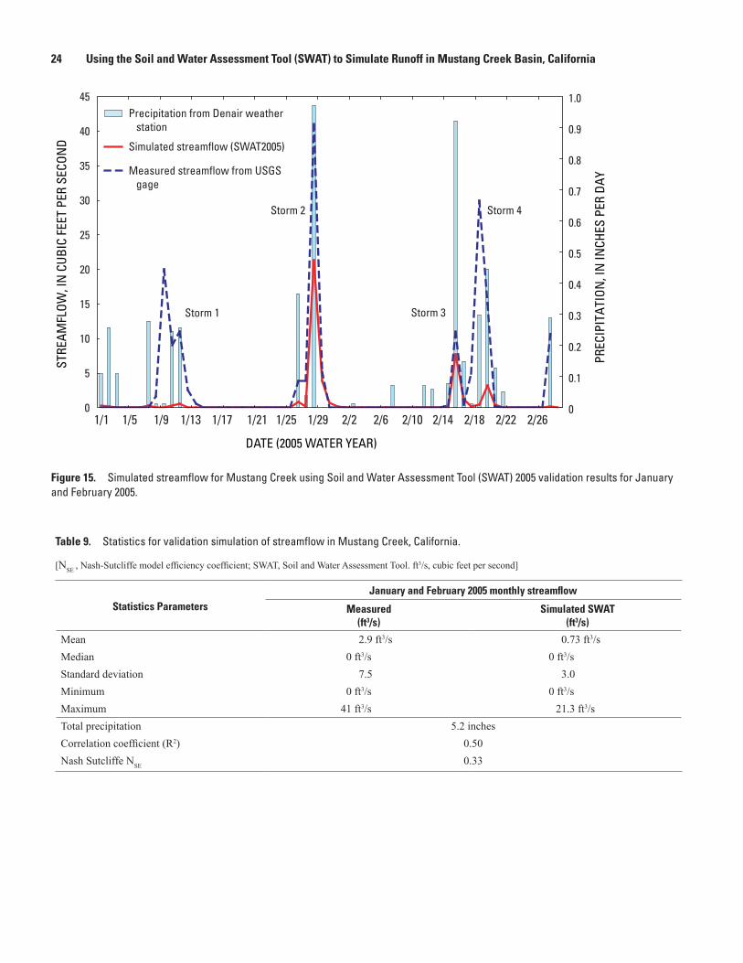
24 Using the Soil and Water Assessment Tool (SWAT) to Simulate Runoff in Mustang Creek Basin, CaliforniaST

REAM

FLOW

, IN

CUB

IC F

EET

PER

SECO

ND

PREC

IPIT

ATIO

N, I

N IN

CHES

PER

DAY

0

5

10

15

20

25

30

35

40

45

1/1 1/5 1/9 1/13 1/17 1/21 1/25 1/29 2/2 2/6 2/10 2/14 2/18 2/22 2/260

0.1

0.2

0.3

0.4

0.5

0.6

0.7

0.8

0.9

1.0

Storm 1

Storm 2

Storm 3

Storm 4

DATE (2005 WATER YEAR)

Precipitation from Denair weather station

Simulated streamflow (SWAT2005)

Measured streamflow from USGS gage

Figure 15. Simulated streamflow for Mustang Creek using Soil and Water Assessment Tool (SWAT) 2005 validation results for January and February 2005.

Statistics Parameters January and February 2005 monthly streamflow

Measured(ft3/s)

Simulated SWAT (ft3/s)

Mean 2.9 ft3/s 0.73 ft3/sMedian 0 ft3/s 0 ft3/sStandard deviation 7.5 3.0Minimum 0 ft3/s 0 ft3/sMaximum 41 ft3/s 21.3 ft3/sTotal precipitation 5.2 inchesCorrelation coefficient (R2) 0.50Nash Sutcliffe NSE 0.33

Table 9. Statistics for validation simulation of streamflow in Mustang Creek, California.

[NSE , Nash-Sutcliffe model efficiency coefficient; SWAT, Soil and Water Assessment Tool. ft3/s, cubic feet per second]

References Cited 25

ConclusionsThe SWAT2005 model was used to simulate streamflow

in Mustang Creek Basin, California, as part of the USGS NAWQA program. The study objective was to determine whether the SWAT model could be used to simulate stream-flow for a basin with an arid-to-semiarid climate, ephemeral flows, and whose land use was predominantly agriculture. The SWAT2005 model was modified to include a depth-to-imper-meable-layer component to account for the impermeable hard-pan layer underlying the study area. This hardpan layer is dis-tributed at different depths and locations throughout the basin. Data from a USGS gaging station were used to investigate the overall hydrologic simulation capability of SWAT2005.

Streamflow data available for calibration and validation were limited — February 2004 (29 days) for calibration and January and February 2005 (58 days) for validation. During the calibration period there were three storm events with pre-cipitation amounts of 0.60, 0.58, and 0.87 in/d, respectively. Results from the calibration period for Mustang Creek showed a reasonably good match between simulated and recorded daily discharge, with Nash-Sutcliffe efficiency (NSE) value of 0.72.

For the validation period, simulated daily discharge was significantly less than the recorded discharge, and the NSE value was an unacceptably poor 0.33. As a result, it was concluded that the SWAT model could not be used to reliably simulate daily discharge for various climatic and land-use scenarios in this particular agricultural basin.

The reasons for the poor simulation performance are varied. The SWAT model was developed for use in basins with perennial flow, and has been used with the most success in simulating monthly or annual mean discharge rather than daily discharge. Mustang Creek drains a small basin and flows only in response to relatively large precipitation events. Accurately simulating relatively infrequent and highly variable daily flows rather than monthly or annual flows is problematic for any continuous flow simulation model.

In addition, the period of available flow record for Mus-tang Creek was very limited. Having a much longer period of daily flow record for both calibration and validation likely would have resulted in better comparisons between recorded and simulated daily flows, because a longer record would not be so affected by a few anomalous high values of discharge as a short record. Not only was the daily flow record short for Mustang Creek, the quality of the recorded daily discharges was poor. The poor-quality streamflow data were the result of very poor and unstable site conditions at the gage location. Poor daily discharge record means that only about 5 percent of the recorded daily discharges are within 15 percent of the true daily discharge values. Such considerable scatter in the recorded daily discharges makes reasonable agreement between simulated and recorded discharges even harder to achieve.

Finally, owing to the fact that precipitation data used for the Mustang Creek model calibration and validation only were available from the Denair weather station located 11 miles west of the study area, and storms are isolated in this loca-tion, data obtained from the Denair weather station may not be representative of weather conditions in the Mustang Creek Basin. This will reflect on the occurrence of runoff in Mustang Creek Basin during the time period when precipitation data were available.

References Cited

Arkley, R.J., 1964, Soil survey of eastern Stanislaus area, Cali-fornia: U.S. Department of Agriculture, Soil Conservation Service, Soil Survey series 1957, no. 20, 160 p.

Arnold, J.G. and Allen, P.M., 1993, A comprehensive surface-ground water flow model: Journal of Hydrology, v. 142, p. 47–69.

Arnold, J.G. and Allen, P.M., 1999, Automated methods for estimating base flow and ground water recharge from streamflow records: Journal of American Water Resources Association, v. 35, no. 2, p. 411–424.

Arnold, J.G. and Fohrer, N., 2005, SWAT2000: current capabilities and research opportunities in applied watershed modeling: Hydrological Processes, v. 19, p. 563–572.

Bingner, R.L., 1996, Runoff simulated from Goodwin Creek watershed using SWAT: Transaction of the American Society of Agricultural Engineering (ASAE), v. 39, no. 1, p. 85–90.

Bingner, R.L., Garbrecht, J., Arnold, J.G., and Srinivasan, R., 1997, Effect of watershed subdivision on simulated run-off and fine sediment yield: Transaction of the American Society of Agricultural Engineering (ASAE), v. 40, no. 5, p. 1329–1335.

Borah, D.K. and Bera, M., 2004, Watershed-scale hydrologic and nonpoint-source pollution models: review of applica-tions: Transaction of the American Society of Agricultural Engineering (ASAE), v. 47, no. 3, p. 789–803.

Bosch, D.D., Sheridan, J.M., Batten, H.L., and Arnold, J.G., 2004, Evaluation of the SWAT model on a coastal plain agricultural watershed: Transaction of the American Society of Agricultural Engineering (ASAE), v. 47, no. 5, p. 1493–1506.

Burow, K.R., Shelton, J.L., Hevesi, J.A., and Weissmann, G.S., 2004, Hydrogeologic characterization of the Modesto area, San Joaquin Valley, California: U.S. Geological Sur-vey Scientific Investigations Report 2004–5232, 53 p.


Capel, P.D., McCarthy K.A., and Barbash, J.E., 2008, National, holistic, watershed-scale approach to understand the sources, transport, and fate of agricultural chemicals: Journal of Environmental Quality, v. 37, p. 983–993.

Chanasyk, D.S., Mapfumo, E., and Willms, W., 2003, Quan-tification and simulation of surface runoff from fescue grassland watersheds: Agricultural Water Management, v. 9, p. 137–153.

Chen, E. and Mackay, D.S., 2004, Effects of distribution-based parameter aggregation on a spatially distributed agricultural nonpoint source pollution model: Journal of Hydrology, v. 295, p. 211–224.

Chu, T.W. and Shirmohammadi, A., 2004, Evaluation of the SWAT model’s hydrology component in the Piedmont phys-iographic region of Maryland: Transaction of the American Society of Agricultural Engineering (ASAE), v. 47, no. 4, p. 1057–1073.

Coffey, M.E., Workman, S.R., Taraba, J.L., and Fogle, A.W., 2004, Statistical procedures for evaluating daily and monthly hydrologic model predictions: Transaction of the American Society of Agricultural Engineering (ASAE), v. 47, no. 1, p. 59–68.

Cotter, A.S., Chaubey, I., Costello, T.A., Soerens, T.S., and Nelson, M.A., 2003, Water quality model output uncer-tainty as affected by spatial resolution of input data: Journal of American Water Resources Association, v. 39, no. 4, p. 977–986.

Dalrymple, T. and Benson, M.A., 1967, Measurement of peak discharge by the slope-area method: U.S. Geological Survey Techniques of Water-Resources Investigations Report, book 3, chap. A2, 12 p.

Davis, S.N. and Hall, F.R., 1959, Water-quality of eastern Stanislaus and northern Merced Counties, California: Stan-ford University Publication, Geological Science, v. 6, no. 1, 112 p.

Di Luzio, M., Arnold, J.G., and Srinivasan, R., 2004, Integra-tion of SSURGO maps and soil parameters within a geo-graphic information system and nonpoint source pollution model system: Journal of Soil and Water Conservations, v. 59, p. 123–133.

Di Luzio, M., Arnold, J.G., and Srinivasan, R., 2005, Effect of GIS data quality on small watershed streamflow and sediment simulations: Hydrological Processes, v. 19, no. 3, p. 629–650.

Du, B., Arnold, J.G., Saleh, A., and Jaynes, D.B., 2005, Development and application of SWAT to landscapes with tiles and potholes: Transactions of the American Society of Agricultural Engineers ACAE, v. 48, no. 3, p. 1121–1133.

Eckhardt, K. and Ulbrich, U., 2003, Potential impacts of climate change on ground water recharge and streamflow in a central European low mountain range: Journal of Hydrol-ogy, v. 284, no. 1–4, p. 244–252.

FitzHugh, T.W. and Mackay, D.S., 2000, Impacts of input parameter spatial aggregation on an agricultural nonpoint source pollution model: Journal of Hydrology, v. 236, p. 35–53.

Fohrer, N., Haverkamp, S., Eckhardt, K., and Frede, H.G., 2001, Hydrologic response to land use changes on the catchment scale: Physics and Chemistry of the Earth, v. 26, no. 7–8, p. 577–582.

Gassman, P.W., Reyes, M.R., Green, C.H., and Arnold, J.G., 2007, The Soil and Water Assessment Tool: Historical development, applications, and future research directions: American Society of Agricultural and Biological Engineers (ASABE), v. 50, no. 4, p. 1211-1250. Available at http://www.card.iastate.edu/environment/items/asabe_swat.pdf

Green, C.H., Tomer, M.D., Di Luzio, M., Arnold, J.G., and James, D., 2006, Hydrologic calibration of the soil and water assessment tool for a large tile-drained watershed in Iowa: Transactions of the American Society of Agricultural and Biological Engineers (ASABE), v. 49, no. 2, p. 411–413.

Gronberg J.M. and Kratzer, C.R., 2006, Environmental setting of the lower Merced River Basin, California: U.S. Geologi-cal Survey Scientific Investigations Report 2006–5152, 27 p.

Hernandez, M., Miller, S.C., Goodrich, D.C., Goff, B.F., Kepner, W.G., Edmonds, C.M., and Jones, K.B., 2000, Modeling runoff response to land cover and rainfall spatial variability in semi-arid watersheds: Environmental Monitor-ing and Assessment, v. 64, p. 285–298.

Heuvelmans, G., Muys, B., and Feyen, J., 2004, Evaluation of hydrological model parameter transferability for simulat-ing the impact of land use on catchment hydrology: Physics and Chemistry of the Earth, Parts A/B/C, v. 29, no. 11–12, p. 739–747.

Holvoet, K., Van Griensven, A., Seuntjens, P., and Vanrol-leghem, P.A., 2005, Sensitivity analysis for hydrology and pesticide supply towards the river in SWAT: Physics and Chemistry of the Earth, v. 30, p. 518–526.

Jha, M., Gassman, P.W., Secchi, S., Gu, R., and Arnold J.G., 2004, Effect of watershed subdivision on SWAT flow, sedi-ment, and nutrient predictions: Journal of American Water Resources Association, v. 40, no. 3, p. 811–825.

http://www.card.iastate.edu/environment/items/asabe_swat.pdf

http://www.card.iastate.edu/environment/items/asabe_swat.pdf

References Cited 27

Kratzer, C.R., Dileanis, P.D., Zamora, C., Silva, S.R., Kendall, C., Bergamachi, B.A., and Dahlgren, R.A., 2004, Sources and transport of nutrients, organic carbon, and chlorophyll-a in the San Joaquin River upstream of Vernalis, California, during summer and fall 2000 and 2001: U.S. Geological Survey Water-Resources Investigations Report 03–4127, 113 p.

Lenhart, T., Eckhardt, K., Fohrer, N., and Frede, H.G., 2002, Comparison of two different approaches of sensitivity analysis: Physics and Chemistry of the Earth, v. 27 (2002), p. 645–654.

Marchand, D.E., and Allwardt, Alan, 1981, Late Cenozoic stratigraphic units, northeast San Joaquin Valley, California: U.S. Geological Survey Bulletin 1470, 70 p.

McElhiney, M.A., 1992, Soil survey for San Joaquin County, California: U.S. Department of Agriculture, Soil Conserva-tion Service, Soil Survey series, 480 p., 37 pl.

Miller, S.N., Kepner, W.G., Mehaffey, M.H., Hernandez, M., Miller, R.C., Goodrich, D.C., Devonald, K.K, Heg-gem, D.T., and Miller, W.P., 2002, Integrating landscape assessment and hydrologic modeling for land cover change analysis: Journal of American Water Resources Association, v. 38, no. 4, p. 915–929.

Nash, J.E. and Sutcliffe, J.V., 1970, River flow forecasting through conceptual models part I—A discussion of prin-ciples: Journal of Hydrology, v. 10, no. 3, p. 282–290.

Neitsch, S.L., Arnold, J.G., Kiniry, J.R., Srinivasan, R., Wil-liams, J.R., 2005, Soil and water assessment tool input/output file documentation, version 2005: 808 east Black-land Road Temple, Texas 76502, Grassland, Soil and Water Research Laboratory, Agricultural Research Service, 506 p.

Panshin, S.Y., Dubrovsky, N.M., Gronberg, J.M., and Doma-galski, J.L., 1998, Occurrence and distribution of dissolved pesticides in the San Joaquin River Basin, California: U.S. Geological Survey Water-Resources Investigations Report 98-4032, 88 p.

Peterson, J.R. and Hamlet, J.M., 1998, Hydrologic calibra-tion of the SWAT model in a watershed containing fragipan soils: Journal of American Water Resources Association, v. 34, no. 3, p. 531–544.

Rosenthal, W.D., Srinivasan, R., and Arnold, J.G., 1995, Alternative river management using a linked GIS-hydrology model: Transaction of the American Society of Agricultural Engineering (ASAE), v. 38, no. 3, p. 783–790.

Saleh, A. and Du, B., 2004, Evaluation of SWAT and HSPF within BASINS program for the Upper North Bosque River watershed in central Texas: Transaction of the American Society of Agricultural Engineering (ASAE), v. 47, no. 4, p. 1039–1049.

Saleh, D.K., 2006, Using the Soil and Water Assessment Tool (SWAT) to simulate runoff in the Mustang Creek Basin, California: Sacramento, California, California State University, M.S. thesis, 84 p.

Santhi, C., Arnold, J.G., Williams, J.R., Dugas, W.A., Srini-vasan, R., and Hauck, L.M., 2001, Validation of the SWAT model on a large river basin with point and nonpoint sources: Journal of American Water Resources Association, v. 37, no. 5, p. 1169–1188.

Soil Survey Staff, Natural Resources Conservation Service, United States Department of Agriculture. U.S. General Soil Map (STATSGO) accessed September, 30, 2006. Available at http://soildatamart.nrcs.usda.gov

Spruill, C.A., Workman, S.R., and Taraba, J.L., 2000, Simu-lation of daily and monthly stream discharge from small watersheds using the SWAT model: Transaction of the American Society of Agricultural Engineering (ASAE), v. 43, no. 6, p. 1431–1439.

Sun, H. and Cornish, P.S., 2005, Estimating shallow ground water recharge in the headwaters of the Liverpool Plains using SWAT: Hydrological Processes, v. 19, no. 3, p. 795–807.

Tolson, B.A. and Shoemaker, C.A., 2004, Watershed model-ing of the Cannonsville Basin using SWAT2000: model development, calibration, and validation for the prediction of flow, sediment, and phosphorus transport to the Cannon-sville Reservoir, version 1.0: Technical Report, School of Civil and Environmental Engineering, Cornell University, 159 p.

University of California, Agriculture and Natural Resources [rev. Nov. 29, 2004], Stanislaus County weather stations: UC IPM Online, available on the web, accessed January 3, 2007, at http://www.ipm.ucdavis.edu/WEATHER/SITES/stanislaus.html

U.S. Geological Survey Land Cover Institute, 1999, National land cover data, digital files. Accessed March 16, 2006, at http://landcover.usgs.gov/natllandcover.php/

Van Griensven, A. and Brauwens, W., 2001, Integral water quality modeling of catchments: Water Science and Tech-nology, v. 43, no. 7, p. 321–328.

Van Griensven, A. and Bauwens, W., 2003, Multiobjective autocalibration for semidistributed water quality models: Water Resources Research, v. 39, no. 12, p. 1348.

Van Griensven, A. and Brauwens, W., 2005, Application and evaluation of ESWAT on the Dender basin and Wister Lake Basin: Hydrological Processes, v. 19, no. 3, p. 827–838.

http://soildatamart.nrcs.usda.gov

http://www.ipm.ucdavis.edu/WEATHER/SITES/stanislaus.html

http://www.ipm.ucdavis.edu/WEATHER/SITES/stanislaus.html

http://landcover.usgs.gov/natllandcover.php/


Van Liew, M.W. and Garbrecht, J., 2003, Hydrologic simula-tion of the Little Washita River experimental watershed using SWAT: Journal of American Water Resources Asso-ciation, v. 39, no. 2, p. 413–426.

Van Liew, M.W., Arnold, J.G., and Garbrecht, J.D., 2003, Hydrologic simulation on agricultural watersheds—choos-ing between two models: Transaction of the American Society of Agricultural Engineering (ASAE), v. 46, no. 6, p. 1539–1551.

Weissmann, G.S., Mount, J.F., and Fogg, G.E., 2002, Glacially driven cycles in accumulation space and sequence stratigra-phy of a stream-dominated alluvial fan, San Joaquin Valley, California: Journal of Sedimentary Research, v. 72, no. 2, p. 240–251.

Williams, J.R. and Hann, R.W., 1978, Optimal operation of large agricultural watersheds with water quality constraints: Texas Water Resources Institute, Technical Report No. 96, Texas A&M University, College Station, Texas.

Williams, J.R., Nicks, A.D., and Arnold, J.G., 1985, Simulator for water resources in rural basins: Journal of Hydrologic Engineering, v. 111, no. 6, p. 970–986.

This page intentionally left blank.

Manuscript approved for publication, June 19, 2008Prepared by the USGS Publishing Network,Publishing Service Center, Sacramento, California

For more information concerning the research in this report, contact the California Water Science Center Director, U.S. Geological Survey, 6000 J Street Sacramento, California 95819 http://ca.water.usgs.gov

Saleh and others—U

sing the Soil and Water A

ssessment Tool (SW

AT) to Simulate Runoff in M

ustang Creek Basin, California—

SIR 2009–5031

Printed on recycled paper

Documents

Using the Soil and Water Assessment Tool (SWAT) to ... · Using the Soil and Water Assessment Tool (SWAT) to Simulate Runoff in Mustang Creek Basin, California By Dina K. Saleh, Charles