Using the Mean Shift Algorithm to Make Post Hoc

Using the Mean Shift Algorithm to Make Post Hoc Improvements to the Accuracy of Eye Tracking Data Based on Probable Fixation LocationsYunfeng Zhang 6/2/10

Directed Research Project (DRP)

University of Oregon

Computer and Information Science Department

Abstract 2

Introduction 2

Systematic Error In Eye Movement Data 4

Eve Movement Data Analysis And Error Correction 7

Eye Movement Data Analysis Procedure 7

Error Correction Based On Hidden Markov Models 8

Error Correction Based On Required Fixation Locations 8

The Experiment With Moving Visual Stimuli 11

A General Method for Removing Systematic Errors 13

Mapping Fixations To Their Probable Locations 14

Visualizing Disparities To Find Their Pattern 14

Applying the Mean Shift Algorithm To Identify the Error Signature 17

Validation of The Method 20

Visualizations of Corrected Data 20

Objective Validation 23

Ground Truth Mappings 23

Comparison to Corrected Data 23

-1-

Possible Extensions 26

Error Signatures Over Time 26

Error Signatures Across Multiple Regions 28

Conclusion 31

Bibliography 32

Appendix 34

Ground Truth Mapping Rules 34

AbstractIf they choose to look for it, eye tracking researchers will almost always see disparities between the participants’ actual gaze locations and the locations recorded by the eye trackers. Sometimes these discrepancies are so great that they dramatically affect the validity of the theoretical and empirical claims made based on the eye tracking data. Much of the disparity is in fact a type of eye tracking error—systematic error—which tends to stay constant over time. A challenge in identifying the size and direction of the systematic error is to determine the participants’ actual gaze locations from the raw data. Mapping gazes to incorrect locations (not their actual locations) would result in misleading disparities and hence inaccurate estimate of the systematic error. In this paper, we propose a general method that can reliably reduce the systematic error and restore the eye movements to their true locations. The method addresses the difficulty in finding mappings between gazes and their correct locations by embracing a typical characteristic of the eye movement data—that the disparities of the correct mappings tend to be similar to each other and hence they form the highest density cluster among all disparities. The method then uses a variant of the mean shift algorithm to locate the cluster and its center, and to reduce the errors by subtracting the center disparity from the eye movement data. This paper presents the method, an extended demonstration, and a validation of the efficacy of the error correction technique.

IntroductionIn usability and psychological studies, researchers often want to know users’ and participants’ internal states of mind in order to understand the efficiency of the interfaces or how humans respond to particular stimuli. States of mind can either be inferred by analyzing a user’s external sequence of actions such as mouse-clicks and key-presses, or they can be revealed through verbal reporting. When using the latter method, the users are asked to say whatever they are looking at, thinking, doing, and feeling. The advantage of the verbal reporting method is that it

-2-

can provide abundant direct information regarding a user’s cognitive processes (Newell & Simon, 1972). But the method also has many drawbacks, e.g., the verbalization might interfere with task processing and hence delay a user’s response time (Ericcson & Simon, 1980). Recording a user’s observable interactions with a device is less intrusive and avoids the problems associated with verbal reports. But there is rarely a precise mapping between people’s internal cognitive processes and mouse clicks and key presses. For example, there might be several approaches to solve an algebra equations, and if researchers only recorded the clicks and key presses, it may be difficult to figure out which approach people used.

As eye trackers become more accurate, researchers increasingly record eye movements as a source of behavioral data (Jacob & Karn, 2003). This particular type of data provides special insight into people’s internal cognitive processes. Eye movement data has two advantages over the traditional behavioral data of reaction time and accuracy. The first advantage is that eye movements are closely related to one important aspect of human information processing—visual attention. Studies have shown that, although people can attend to stimuli that are not in the foveal vision (also known as covert attention), when doing real-world tasks, they tend to move their eyes to things that they are attending to (Findlay & Gilchrist, 2003). None of the traditional behavioral data can map so closely between external actions and internal states of mind. The second advantage of eye movement data is that the duration of a fixation (in which the gaze is maintained around a single location) generally ranges from 150 ms to 600 ms, which provides for many tasks a much smaller grain size of temporal data points than provided by mouse clicks, key presses, or reaction time data. Smaller time scales isolate individual strategic decisions and hence permit researchers to more easily infer specific strategies that people adopt (Newell, 1990). For example, eye movement data for solving an algebra equation can show the order in which the participant looked at the numbers and variables, and how long he or she spent on each, which can in turn reveal the task strategy (Salvucci & Anderson, 2001). Due to the above reasons, eye tracking is used increasingly in usability studies to replace or complement verbal reports (Goldberg et al., 2002; Burke, Hornof, Nilsen & Gorman, 2005).

However, researchers should not be overly optimistic about using eye tracking as an easy means to answer difficult questions, because eye tracking data is inherently noisy. Unlike mice, which are directly controlled by users and thus reflect the actual locations that users are pointing to, eye trackers estimate people’s gaze locations through indirect measures. For example, video-based eye trackers, which are most widely used in usability studies, work by reflecting infrared light onto the corneal, and use the vector between the pupil-center and corneal reflection to calculate gaze locations. The computer vision algorithms used in the procedure are not perfect and errors occur. As well, some eye trackers still cannot handle head movements very well (Li, Babcock & Parkhurst, 2006).

There are generally three types of eye tracking errors (Hornof & Halverson, 2002). First, the eye tracker may not be able to acquire an image of the eyes (e.g. when the users are not sitting at an appropriate distance) which results in complete data loss. Second, random error occur due to inaccurate estimations of gaze locations. These random errors are often less than 0.5º of visual

-3-

angle (the angle that a viewed object subtends at the eye) and can be reduced by averaging the gaze points (LC Technologies, 2000). The last type of eye tracking data error—systematic errors or bias errors—result from bad calibrations, head movements, astigmatism and other sources, and stay constant from time to time (LC Technologies, 2000). Systematic errors can sometimes reach many degrees of visual angle. The good news is that systematic errors can be systematically removed with techniques such as that presented here.

The remainder of the article will discuss the issues of systematic errors, including their influences on eye movement data analysis; some previous methods that can deal with these errors; and a new method which can reliably reduce systematic errors.

Systematic Error In Eye Movement DataFigure 1 illustrates what systematic error looks like. The data are from a test of the Tobii T60 eye tracker, which has a reported accuracy of 0.5º of visual angle and is widely used in usability studies. In the test, the participant was asked to look at the four corners of the rectangle consecutively. But unlike a typical experiment, the participant was asked to adjust her head position in order to test the sensitivity of the tracking accuracy to head movements. As can be seen in Figure 1, the four fixations are all somewhat above the corners by a similar amount of disparity. The systematic errors that can be seen in the figure is very large—roughly 2.3º of visual angle on average, well over the manufacture’s stated accuracy. The figure shows a typical pattern in data with systematic errors—the recorded eye movement data are all altered by a similar vector.

Although systematic errors are common in eye tracking data, they are rarely reported in any form (as in Blignaut, Beelders & So, 2008; Smith, Ho, Ark & Zhai, 2000). Yet, in any scientific measurement it is critical to know the accuracy of the measuring instrument. If no error report is provided based on the actual data collected, it is difficult to determine whether the study examined, explored, or realized the severity of the error, and whether the data are truly accurate.

Figure 1. The participant looked at the four corners of the rectangle, but the eye tracking data are all above the corners due to systematic errors. Circles represent fixations.

-4-

The error may not be a problem in usability studies in which the areas of interests (AOIs) extend to a large area (e.g. 8º of visual angle) and are also separated by a large distance. But in studies that pertain to reading, visual search of dense displays, and cockpit usability evaluation, researchers often want to know precisely at what objects participants looked. The visual stimuli in these studies (such as labels and buttons) and the space between them tend to be only about 1º to 3º of visual angle. In these circumstances, if the systematic error is as large as 2º of visual angle, a fixation is likely to be incorrectly interpreted on an object adjacent to the one that a participant actually looked at. For example, in Figure 1, if only the lower two fixations are recorded or the task requirement—look at four corners—is not known, one would think that the lower two fixations were on the top corners because they appear closer to the top corners. However, they are in fact on the bottom corners, just shifted by systematic error. Thus, it is perhaps impossible to draw any reliable conclusions in an eye tracking study without first addressing the systematic error. Ignoring the error can dramatically affect the validity of empirical and theoretical claims made based on the eye tracking data.

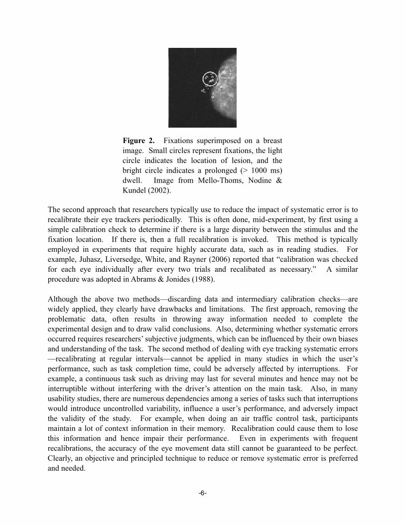
When researchers indeed find systematic error in their data, or realize that it is possible that such errors might occur in their experiments, they tend to address the errors in two ways. First, they exclude the eye tracking data from the trials in which they have found errors. Many studies adopt this approach. For instance, Mello-Thoms, Nodine & Kundel (2002) conducted an eye tracking experiment to examine how radiologists search breast cancer. They found in some trials, such as shown in Figure 2, the lesion did not attract any fixations, whereas the dark background was fixated for a fairly long time. The eye movement data of such trails were excluded from the analysis. Although Mello-Thoms et al. did not attribute these data to systematic error in the eye tracker, it is likely this is the source, because there are no stimuli on the dark background that could attract and maintain visual attention for such a long time. One might argue that the participants may have used covert attention here, but task constraints and human physiology would motivate fixations directly on the relevant visual objects (Findlay & Gilchrist, 2003).

-5-

The second approach that researchers typically use to reduce the impact of systematic error is to recalibrate their eye trackers periodically. This is often done, mid-experiment, by first using a simple calibration check to determine if there is a large disparity between the stimulus and the fixation location. If there is, then a full recalibration is invoked. This method is typically employed in experiments that require highly accurate data, such as in reading studies. For example, Juhasz, Liversedge, White, and Rayner (2006) reported that “calibration was checked for each eye individually after every two trials and recalibated as necessary.” A similar procedure was adopted in Abrams & Jonides (1988).

Although the above two methods—discarding data and intermediary calibration checks—are widely applied, they clearly have drawbacks and limitations. The first approach, removing the problematic data, often results in throwing away information needed to complete the experimental design and to draw valid conclusions. Also, determining whether systematic errors occurred requires researchers’ subjective judgments, which can be influenced by their own biases and understanding of the task. The second method of dealing with eye tracking systematic errors—recalibrating at regular intervals—cannot be applied in many studies in which the user’s performance, such as task completion time, could be adversely affected by interruptions. For example, a continuous task such as driving may last for several minutes and hence may not be interruptible without interfering with the driver’s attention on the main task. Also, in many usability studies, there are numerous dependencies among a series of tasks such that interruptions would introduce uncontrolled variability, influence a user’s performance, and adversely impact the validity of the study. For example, when doing an air traffic control task, participants maintain a lot of context information in their memory. Recalibration could cause them to lose this information and hence impair their performance. Even in experiments with frequent recalibrations, the accuracy of the eye movement data still cannot be guaranteed to be perfect. Clearly, an objective and principled technique to reduce or remove systematic error is preferred and needed.

Figure 2. Fixations superimposed on a breast image. Small circles represent fixations, the light circle indicates the location of lesion, and the bright circle indicates a prolonged (> 1000 ms) dwell. Image from Mello-Thoms, Nodine & Kundel (2002).

-6-

In this paper, we propose a post hoc method to reduce the systematic error in eye movement data. Because the error correction is done after collecting data, it would not interfere with task execution. This method also provides an objective measure of the accuracy of the raw data.

Eve Movement Data Analysis And Error CorrectionThis section introduces two previous methods that have been proposed to deal with error in eye movement data. The first method calculates a fixation’s true location using not only the fixation’s recorded location but also he fixation’s role in task execution (Salvucci & Anderson, 2001). The second method studies the nature of the systematic errors and reduces them accordingly (Hornof & Halverson, 2002). The error correction technique presented in this paper follows the general approach of the second.

Eye Movement Data Analysis Procedure

Before delving into the details of the two error correction methods, we shall first revisit the two basic stages of automated eye movement data analysis. This brief introduction provides a context that helps to show when the error correction should be carried out and how much should be done to rigorously analyze eye movement data.

Fixation Detection. The first stage of eye movement data analysis is to group the raw gaze samples into fixations. The raw data collected by eye trackers are sampled at a constant rate, often 60 Hz. In some experiments, researchers can work directly with the raw gaze samples. But generally, the samples are grouped into fixations. There are several algorithms for detecting fixations (Salvucci & Goldberg, 2000). The dispersion-based and velocity-based algorithm are the two main ones. The dispersion-based algorithm has two parameters: maximum dispersion size and minimum fixation duration. The velocity-based algorithm has one parameter: the velocity threshold. When analyzing data, it is wise to try a range of values for these parameters to determine the optimum settings for different tasks. Karsh & Breitenbach (1983) provide an excellent illustration of how different parameter settings of the dispersion-based algorithm can dramatically affect the fixation detection outcome.

Fixation Assignment. The second stage of automated eye movement analysis is to find each fixation’s target object, i.e. to assign fixations to their intended stimuli. The most commonly used fixation-assignment method is to map each fixation to its nearest object. The idea of this method is easy to understand: The closer a fixation is to an object, the better the object is perceived. However, when the eye movement data have systematic errors, this nearest-object assignment method could very likely make mistakes, because the fixations are not at their actual locations. For example, if this fixation assignment method is used for the eye movement data in Figure 1, both two fixations on the left would be assigned to the top-left corner of the rectangle,

-7-

and the two fixations on the right would be assigned to the top-right corner. Here, the systematic error has caused two wrong mappings.

Error Correction Based On Hidden Markov Models

Based on hidden Markov models, Salvucci and Anderson (2001) designed a fixation assignment method that is resistant to the effect of eye tracking error, but the method has a few drawbacks. In this method, the strategies that might be used to successfully complete the task, which can be obtained by task analysis, are formally coded into a hidden Markov model. Then the fixation sequences are compared with the hidden Markov model to obtain fixation assignments. Two factors determine a fixation’s assignment: (a) the fixation location and (b) the probability that the fixation would be on a stimulus at a point in time according to the model. Thus, even if a fixation is further from its intended stimulus than it is from another stimulus, perhaps due to the systematic error, it will still be assigned to the intended visual stimulus if this match yields a higher probability in the hidden Markov model. One of the important contributions of Salvucci and Anderson’s method is that it takes advantage of a powerful mathematic tool, hidden Markov modeling, to formally represent possible strategies. However, it is complex to implement a hidden Markov model and sometimes impossible to decide what transition probabilities should be used. There is little evidence in the literature that this approach is routinely used in any eye tracking studies, even for those subsequently conducted by the creators of the technique themselves. The error correction method presented here offers an easier-to-use alternative.

Error Correction Based On Required Fixation Locations

This section discusses Hornof & Halverson’s (2002) error correction method, including the concept of required fixation locations as well as some limitations of this method. The error correction method presented in this paper takes a similar approach, but offers substantial improvements. Similarities include: First, both methods reduce the systematic errors before the fixation assignment stage; this way, the nearest-object fixation assignment method would less likely make many wrong mappings. Second, both methods extract the size and direction of the systematic errors by studying the disparities between fixations and their intended locations. The difference is that Hornof & Halverson’s method chooses the fixations more conservatively and thus has some limitations as discussed later, whereas the technique presented here can estimate locations for most of the fixations.

In Hornof & Halverson (2002), the authors thoroughly studied the nature of systematic errors in a set of eye tracking data collected from a visual search experiment. They found that the systematic error tends to be constant within a region of the display for each participant. Specifically, the magnitude of the disparities between the target visual stimuli and the corresponding fixations were “somewhat evenly distributed around 40 pixels (about 1º of visual angle) and that most were between 15 and 65 pixels”. The variation in the magnitude of the disparity was even smaller if broken down by participant. Horizontal and vertical disparities remained somewhat constant for each participant. Thus, systematic error was not randomly

-8-

distributed across all directions or sizes but was, as the name implies, systematic. The error was illustrated with a vector plot that forms each participant’s error signature in which the vectors change gradually across the display area (Figure 3).

Because the systematic error is relatively constant within a region, it is possible to reduce the error for each region—and even each point—individually. The key idea of Hornof and Halverson (2002) is that researchers can determine how to offset each recorded fixation by calculating a weighted average of the error vectors that are closet to that recorded fixation, and by shifting that fixation based on the error signature calculated for that location. Consequently, the gaze points are shifted toward their true locations, and systematic error is reduced. For example, in Figure 3, the eye movement data that are close to each column would be corrected based on the vectors of the nearest column. Thus, the eye movement data for fixations near the left column should be shifted upward, and those near the middle and right column should be moved up and to the right.

To obtain an accurate estimate of the direction and size of the systematic error, the disparities used to generate the error signatures must capture the difference between recorded fixations and their true intended stimuli, rather than just the closet and potentially unrelated stimuli. These correct mappings are not easy to acquire considering that the uncorrected data may have large systematic errors. To solve this problem, Hornof and Halverson (2002) developed the concept of required fixation locations (RFLs), which are locations on the screen that the analyst can be relatively certain that a participant fixated at a specific point in time, provided that the participant completed the trial accurately. Some RFLs are easy to find. For example, an RFL can be a set of crosshairs that a participant is specifically instructed to fixate. However, not all tasks permit such explicit RFLs. Researchers need to conduct thoughtful and accurate task analyses to find opportunities in which participants are implicitly required to fixate an RFL. For instance, for a participant to correctly key-in a small number that is displayed on a visual target, the participant must fixate that target at some point in the trial. In Hornof and Halverson’s visual search experiment, the to-be-found target items served as implicit RFLs. It was reasonable to assume,

Figure 3. A screen shot of visual search targets with one participant’s error signatures (the vector plot). Notice that the error signature gradually changs for different display locations. Image from Hornof & Halverson (2002).

-9-

based on task design (such as monetary rewards for fast responses, and no time pressure between trials), that participants were looking at the target when they clicked on it with the mouse.

Hornof and Halverson’s RFL technique successfully reduc systematic error for a visual search experiment in which all visual stimuli are fixed on a grid. As shown in Figure 4, the eye movement data after error correction (in black) is more plausible than the raw data (in gray), given the assumption of active vision (that the point-of-gaze is directed to visually-attended objects) because all of the corrected fixations now land on the labels. Note that the eye movement data shown in Figure 4 were corrected only using the disparities in the final fixation of each trial (in Figure 4, the large fixation near the RUB label). Across the experiment, the mean uncorrected systematic error size was about 0.73º of visual angle. Considering that the labels in their experiment only subtend 1º of visual angle, and that there is no space between adjacent labels, reducing systematic error by 0.73º could have been critical for the subsequent data analysis.

Hornof and Halverson’s method could potentially be used in a wide range of eye tracking studies, but it has four limitations. First, it still relies on a researcher’s subjective judgement to determine the potential RFLs. In Hornof and Halverson’s visual search experiment, the RFLs are the targets that were being clicked by the mouse. This way of finding RFLs will not always be practical or possible because some tasks may not need a mouse at all. Second, the way that they chose RFLs is based on a reasonable task analysis—people tend to look at the objects that they select—but the method is a bit conservative in that it limits RFLs to items selected with a mouse while under time pressure. Other ways of choosing RFLs will be needed for different tasks, but a tradeoff exists—the more confident researchers want to be about the true locations of fixations, the fewer RFLs they can identify. Third, defining RFLs for moving visual stimuli is even harder because it requires knowing what objects participants may look at and at exactly what time would they look at them. Fourth, the existing RFL technique does not reliably correct eye movement data when the systematic error changes over time. Because of the above limitations,

Figure 4. Light gray circles indicate fixation data recorded by the eye tracker, and the black circles indicate the data after error correction. Circle diameter reparents fixation duration. Image from Hornof & Halverson (2002).

-10-

exploration is needed to find more opportunities not for required fixation locations but for probable fixation locations.

With regards to the problem of not reliably correcting errors that change over time, Hornof & Halverson (2002) stated: “An interesting question is whether we could take the analysis further and determine how a participant’s error signature changes over time—from calibration to calibration or even from trial to trial.” (p. 600) The assumption that error signatures stay constant may hold for short experiments, it is not clear how the systematic errors will change for long experiments. The fact that eye tracking accuracy deteriorates over time (such as implied in experiments that invoke recalibration at regular intervals) suggests that error signatures should also change over time. One reason that Hornof and Halverson did not address this issue is perhaps because detecting a change in an error signature across a period of time would require a substantial number of RFLs across the task display for numerous windows of time and, as discussed before, Hornof and Halverson chose their RFLs conservatively and hence somewhat sparsely.

Hornof and Halverson’s approach is appropriate for an initial exploration of the RFL technique, but the method needs to be extended to accommodate tasks in which visual objects can appear anywhere on the display (not just on a grid) and even move across the display during a task. The extensions to the RFL technique presented here are developed in the context of exactly such a task, the Naval Research Laboratory dual task, discussed next.

The Experiment With Moving Visual StimuliThis section describes the Naval Research Laboratory (NRL) dual task experiment, which was the context in which the new error correction technique was developed to address the four limitations of the existing RFL technique discussed in the previous section. The NRL dual task experiment has many moving visual stimuli, and hence it is very difficult to apply the existing RFL technique as-is to the eye tracking data from the experiment. However, good eye tracking data for the task could reveal important details and insights regarding fundamental human information processing.

The NRL dual task experiment consists of two subtasks performed in parallel: the classification task and the tracking task. Figure 5 shows an overview of the task display. In the classification task, the participants examine blips (the small icons on the left display in Figure 5) that move down the screen, and key-in the blip number (the digit displayed on the icon) followed by “H” or “N” for a hostile or neutral classification. The classification can be keyed-in after the blip changes from black to green, red or yellow, indicating that it is active and “ready to be classified.” The hostility can be determined by studying the blip’s color: Red indicates hostile and green indicates neutral; if the blip is yellow, the participant needs to study its shape, speed and direction to determine its hostility. Fifty-seven blips are grouped into 16 waves, in which 1,

-11-

2, 4, 6, or 8 blips are visible at the same time. In the tracking task (on the right display in Figure 5), the participant simply uses a joystick to keep the circle on the moving target.

Figure 5 shows how the two task displays are arranged on a single monitor, with the classification task displayed on the left and the tracking task displayed on the right. Other conditions such as the presence of sound and peripheral visibility are manipulated, but they are not terribly relevant to the development or evaluation of the eye movement data correction method. See Hornof, Zhang & Halverson (2010) for a more detailed description of the experiment.

Twelve participants from the University of Oregon and surrounding communities successfully completed the experiment. They completed four sessions of the experiment on each of three consecutive days. Participants were financially motivated to perform as quickly as possible while maintaing very high accuracy. Given the practice and motivation, participants’ performance by day three approach that of an expert.

The eye tracking instrumentation settings were kept as consistent and reliable as possible to reduce systematic error. The screen resolution was set to 1280x1024. A chinrest was used to maintain a constant eye position 610 mm from the display. One degree of visual angle extended to about 40 pixels on the display. The size of blip icons was 32x32 pixels, i.e. 0.8ºx0.8º of visual angle. Blip movements were designed to maintain a 2º separation. Eye movements were recorded using an LC Technologies dual camera eye tracker, which has a sampling rate of 120 Hz. Each session of the experiment took about 8 minutes on average to complete. Because the task is continuous across these 8 minutes, the eye tracker cannot be recalibated during a session. Despite all of these efforts to reduce systematic error, when collecting eye movement data for such a long duration without recalibration, systematic errors are still likely to occur.

Task-Constrained Interleaving of Perceptual and Motor Processes

in a Time-Critical Dual Task as Revealed Through Eye Tracking

Anthony J. Hornof ([email protected])Yunfeng Zhang ([email protected])

Computer and Information Science, University of OregonEugene, OR 97403 USA

Abstract

A multimodal dual task experiment that contributed to the original development and tuning of the EPIC cognitive architecture is revised and revisited with the collection of new high fidelity human performance data, most notably detailed eye movement data, that reveal the complex overlapping of perceptual and motor processes within and between the two competing tasks. The data permit a new detailed evaluation of assumptions made in previous models of the task, and contribute to the development of new models that explore opportunities for overlapping visual-perceptual, auditory-perceptual, ocular-motor, and manual-motor activities. Three models are presented: (a) A hierarchical, task-switching model in which each task locks out the other; the model explains reaction time but does not account for eye movement data. (b) A maximum-overlap perceptually-driven model that maximizes parallel processing and predicts the trends in the eye movement data, but performs too quickly. (c) A moderately-overlapped perceptually-driven model that introduces task-motivated constraints and predicts both reaction time and eye movement data. The best-fitting model demonstrates the complex task-constrained interleaving of perceptual and motor processes in a time-pressured dual task.

Keywords: Cognitive strategies, EPIC cognitive architecture, eye tracking, multimodal dual task, multitasking.

Introduction

A critical task domain for the research enterprise of cognitive modeling—the practice of building computer programs that account for aspects of human information processing—is that of multimodal (auditory and visual) multitasking. Psychologists and cognitive modelers puzzle over the question of how people engage in two or more time-pressured tasks that compete for perceptual, cognitive, and motor processes, such as for air-traffic control or in-car navigation (Byrne & Anderson, 2001; Howes, Lewis, & Vera, 2009; Meyer & Kieras, 1997; Salvucci & Taatgen, 2008). Gaining an understanding and ability to predict aspects of multimodal multitasking is of critical scientific and practical importance. This paper advances an understanding of such tasks by presenting cognitive models of time-critical multimodal multitasking and evaluates these models in great detail using eye tracking data.

The Time-Critical Multimodal Dual Task

An earlier version of the experiment that forms the basis of this theoretical exploration was conducted in the early 1990s at the Naval Research Laboratory (NRL) (Ballas, Heitmeyer, & Perez, 1992). The experiment produced

human speed and accuracy data that proved useful for developing detailed computational cognitive models of dual task performance (Kieras, Ballas, & Meyer, 2001). In the NRL dual task, participants use a joystick to track a moving target on one display and, in parallel, key-in responses to objects that appear on a secondary “radar” display. This paper presents an experiment that extends the original NRL dual task in numerous important ways, including that (a) eye movements are recorded, (b) eye tracking is used in some conditions to hide objects on the not-currently-looked-at display, (c) auditory cues relate more directly to required responses, and (d) participants are rigorously trained, financially motivated, and given extensive feedback so that performance approaches that of an expert.

Figure 1 shows an overview of the two displays used in the multimodal dual task modeled in this paper. Two tasks (or subtasks) were performed in parallel: a tracking task and a radar classification task. The tracking task consisted of keeping a small circle on a moving target using a joystick. When the circle was positioned as such, it turned green, and the participant was financially rewarded at a constant rate. The classification task consisted of monitoring groups of small icons or “blips” (fifty-seven blips across an nine-minute scenario) that moved down the screen, and keying-in the blip number and “hostile” or “neutral” as soon as the blip changed from black to red, green, or yellow, indicating that it was “ready to classify”. At the point a blip ready to classify, a financial bonus was awarded though it diminished at a constant rate until the blip was keyed-in, or classified. Red blips were hostile; green were neutral; yellow blips were classified based on their shape, speed, and direction, following practiced rules.

Submitted to ICCM 2010 – International Conference on Cognitive Modeling – Please do not cite or distribute.

1

Figure 1: An overview of the visual and auditory displays and input devices used in the multimodal dual task.

21 3

4 5 6

7 8 9

H

Nchproducts.com

Classification TaskTactical Radar Display

Tracking Task

Figure 5. An overview of the components and input devices of the dual task experiment. Image from Hornof & Zhang (2010, to appear).

-12-

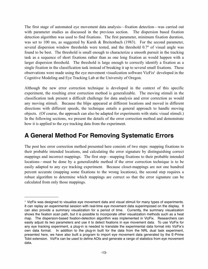
The first stage of automated eye movement data analysis—fixation detection—was carried out with parameter studies as discussed in the previous section. The dispersion based fixation detection algorithm was used to find fixations. The first parameter, minimum fixation duration, was set to 100 ms, as suggested by Karsh & Breitenbach (1983). For the second parameter, several dispersion window thresholds were tested, and the threshold 0.7º of visual angle was found to be best. The threshold is small enough to characterize a smooth pursuit in the tracking task as a sequence of short fixations rather than as one long fixation as would happen with a larger dispersion threshold. The threshold is large enough to correctly identify a fixation as a single fixation in the classification task instead of breaking it up to several small fixations. These observations were made using the eye movement visualization software VizFix1 developed in the Cognitive Modeling and Eye Tracking Lab at the University of Oregon.

Although the new error correction technique is developed in the context of this specific experiment, the resulting error correction method is generalizable. The moving stimuli in the classification task present a difficult challenge for data analysis and error correction as would any moving stimuli. Because the blips appeared at different locations and moved in different directions with different speeds, the technique entails a general approach to handle moving objects. (Of course, the approach can also be adapted for experiments with static visual stimuli.) In the following sections, we present the details of the error correction method and demonstrate how it is applied to the eye tracking data from the experiment.

A General Method For Removing Systematic ErrorsThe post hoc error correction method presented here consists of two steps: mapping fixations to their probable intended locations, and calculating the error signature by distinguishing correct mappings and incorrect mappings. The first step—mapping fixations to their probable intended locations—must be done by a generalizable method if the error correction technique is to be easily adapted to any eye tracking experiment. Because closet-mappings are not one hundred percent accurate (mapping some fixations to the wrong locations), the second step requires a robust algorithm to determine which mappings are correct so that the error signature can be calculated from only those mappings.

-13-

1 VizFix was designed to visualize eye movement data and visual stimuli for many types of experiments. It can replay an experimental session with real-time eye movement data superimposed on the display. It can also provide a summary visualization for a period of time. Currently, the summary visualization shows the fixation scan path, but it is possible to incorporate other visualization methods such as a heat map. The dispersion-based fixation-detection algorithm was implemented in VizFix. Researchers can easily adjust its two parameters and use it to detect fixations in eye movement data. To use VizFix for any eye tracking experiment, a plug-in is needed to translate the experimental data format into VizFixʼs own data format. In addition to the plug-in built for the data from the NRL dual task experiment, presented here, we have also built a program to import eye movement data generated by the E-Prime Tobii extension. VizFix can be used to define AOIs and generate a range of statistics from eye movement data.

Mapping Fixations To Their Probable Locations

A nearest-object fixation assignment method is developed to identify the probable location of each fixation. This method maps each fixation to its closet stimulus and uses the center of the stimulus as the probable intended location, provided that the distance between them does not exceed a threshold. The threshold parameter helps exclude rare situations in which a short fixation was not on any stimulus but just landed on the blank background. Another way to think about the threshold is that it is the longest distance from an object and the point of gaze such that the high resolution vision at the point of gaze can still encode the object. To estimate this distance, researchers should consider two factors—the theoretical longest distance from the point-of-gaze at which an object can be discerned, and the maximum size of the systematic errors. The first factor depends on the feature to be encoded and the size of the object. The second factor—the maximum size of the systematic errors—should be considered because in the uncorrected data, the distance between a fixation and its intended location is now extended by the systematic error. The sum of the two factors is the maximum possible distance between a fixation and its intended stimulus in the uncorrected data. In the NRL dual task experiment, the participant needs to study the small digit (less than 0.8º) on the blip. Because the small character is only easily discriminable in the fovea, the first factor—the theoretical longest distance between a fixation and a target object—is set to 1º (Kieras & Meyer, 1997). After examining the data visualization, the maximum systematic error was estimated to be 3º. Thus, the longest distance between a fixation and its target object is set to 4º in the NRL dual task experiment data.

There are two reasons to use the nearest-object fixation assignment method to find the probable locations of fixations. First, the method is applicable to virtually all experiments without the need of careful task analysis. Second, because nearly all fixations are assigned a mapping, the method can generate a substantial number of mappings which enable a more finely-tuned error correction for different screen regions and time periods. Also, a more reliable error signature can be acquired by incorporating more disparities from the mappings.

The downside of the nearest-object fixation assignment method is that it can assign many incorrect mappings due to systematic error—the very error that the technique is designed to reduce. However, it is exactly for this reason that the second step of the error correction procedure is introduced—to exclude the effect of the incorrect mappings. Note that at the error correction stage, fixations are not really assigned to visual objects. These mappings are merely used to determine the pattern of the systematic error. The actual fixation assignment will be carried out after reducing the error.

Visualizing Disparities To Find Their Pattern

Visualizing disparities is not a required step for applying the error correction method, but it helps to reveal the patterns of disparities and is thus useful for developing the method, especially for finding an appropriate algorithm to exclude the effect of incorrect mappings. Figure 6 shows a disparity graph for a session of the NRL dual task experiment in which the disparities are plotted

-14-

in terms of their x and y deviations. In this graph, the nearest-object fixation assignment method has found 233 disparities (black dots). Among them, there is a cluster of dots around (10, 35) which occupies only a small area of the graph. Note that if there were no systematic errors in this data, all the fixations should be very close to their targets and so the disparities should be around (0, 0). Although there is no clear boundary between the cluster and other dots, the cluster is apparently much denser than other area. The graph suggests that a large portion of the fixations in that session are off their targets by roughly 10 pixels horizontally and 35 pixels vertically.

The disparity graphs for other sessions of the experiment have a similar pattern—one small area is crowded with dots and other dots are sparsely scattered over the graph. This pattern emerges because the fixation assignment method finds many correct mappings and some incorrect mappings. For the correct mappings, the disparities tend to be similar, hence they form a cluster in the graph, and the vector from the origin to the center of the cluster is the error signature of the systematic error. For the incorrect mappings, the disparities would not follow any certain pattern. Thus they are randomly distributed over many directions. Understanding this particular pattern of disparities would help enormously with finding a suitable algorithm that would be robustly remove the effect of the wrong mappings.

-15-

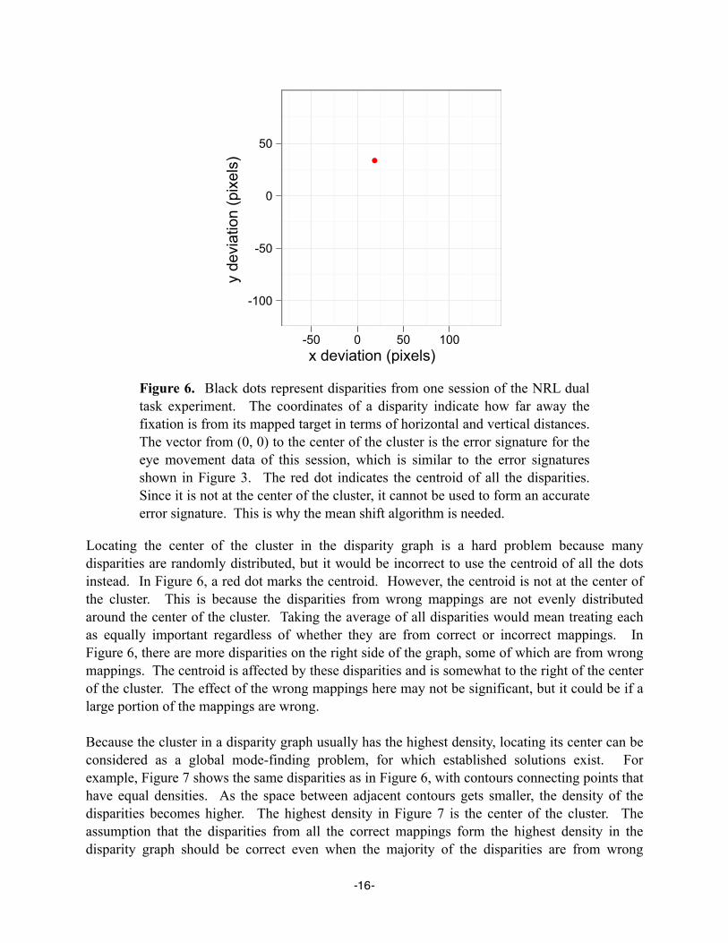
Locating the center of the cluster in the disparity graph is a hard problem because many disparities are randomly distributed, but it would be incorrect to use the centroid of all the dots instead. In Figure 6, a red dot marks the centroid. However, the centroid is not at the center of the cluster. This is because the disparities from wrong mappings are not evenly distributed around the center of the cluster. Taking the average of all disparities would mean treating each as equally important regardless of whether they are from correct or incorrect mappings. In Figure 6, there are more disparities on the right side of the graph, some of which are from wrong mappings. The centroid is affected by these disparities and is somewhat to the right of the center of the cluster. The effect of the wrong mappings here may not be significant, but it could be if a large portion of the mappings are wrong.

Because the cluster in a disparity graph usually has the highest density, locating its center can be considered as a global mode-finding problem, for which established solutions exist. For example, Figure 7 shows the same disparities as in Figure 6, with contours connecting points that have equal densities. As the space between adjacent contours gets smaller, the density of the disparities becomes higher. The highest density in Figure 7 is the center of the cluster. The assumption that the disparities from all the correct mappings form the highest density in the disparity graph should be correct even when the majority of the disparities are from wrong

Figure 6. Black dots represent disparities from one session of the NRL dual task experiment. The coordinates of a disparity indicate how far away the fixation is from its mapped target in terms of horizontal and vertical distances. The vector from (0, 0) to the center of the cluster is the error signature for the eye movement data of this session, which is similar to the error signatures shown in Figure 3. The red dot indicates the centroid of all the disparities. Since it is not at the center of the cluster, it cannot be used to form an accurate error signature. This is why the mean shift algorithm is needed.

x deviation (pixels)

y d

evia

tion (

pix

els

)

-100

-50

0

50

-50 0 50 100

-16-

mappings, because the wrong disparities tend to be scattered all over the graph and thus have lower densities.

The global mode-finding problem has already been studied in other areas, and the error correction method adopts one of the existing solutions—the annealed mean shift algorithm (Shen, Brooks & Hengel, 2007). The following section first presents the standard mean shift procedure, which is used to find the local modes, and then discusses how the annealed mean shift algorithm can reliably find the global mode.

Applying the Mean Shift Algorithm To Identify the Error Signature

A procedure called the mean shift algorithm which is used in computer vision for feature space analysis (Comaniciu & Meer, 2002) can be adapted to solve the problem of identifying the error signature. Although the disparities of the eye movement data do not follow a certain distribution, the mean shift algorithm can still work because it does not rely on a particular distribution. The mean shift method is derived from a nonparametric density estimator, specifically the kernel density estimator. Because nonparametric statistics can work with any distribution, it makes the error correction technique more robust as it now relies on fewer assumptions.

The kernel density estimation method works by estimating the density at a given location from its neighboring points. The size of the “neighborhood” is controlled by a bandwidth matrix H and the weights associated with the neighboring points are determined by the kernel function.

Figure 7. Densities of the disparities in Figure 6. Blue contours connect equal density points. The cluster center has the greatest density, and is likely to be the error signature from (0, 0).


y d

evia

tion (

pix

els

)

-100

-50

0

50

-50 0 50 100

-17-

With some simplification on the bandwidth matrix H, the following kernel density estimator is obtained:

where the xi terms are n data points in the d-dimensional space Rd, h is a scalar derived from the bandwidth matrix H, k(⋄) is the profile of the actual kernel function, and ck is a normalization constant. In practice, two kernel functions have been widely applied, the Epanechnikov kernel and the multivariate normal kernel. Given a d-dimensional point x, the above formula returns the density estimation at point x.

Once the density function is acquired through the kernel density estimation procedure, the local modes (local maximum points) can be found by setting the gradient equal to zero. This is equivalent to setting the following term to zero:

where g(x) = –k´(x), and mG(x) is the mean shift vector. Starting from any random location, the following scheme can be applied iteratively to stop at a local maximum point:

For a more detailed discussion of the standard mean shift procedure, see Comaniciu & Meer (2002).

The standard mean shift procedure has been proven to reliably find local mode points, but a better method is needed in order to find the global mode, as is required here to determine the error signature. In the context of eye movement error correction, a local mode point could potentially be the center of a small cluster formed by wrong disparities, and if the mean shift procedure stops at such a point instead of the global mode, it would generate a wrong error signature. To combat this, we use the annealed mean shift algorithm, presented by Shen, Brooks & Hengel (2007), which finds the global mode reliably.

The annealed mean shift procedure finds the global mode by applying multiple passes of the standard mean shift process with a sequence of decreasing bandwidths to gradually zoom in on the global mode. Initially a very large bandwidth hM is used, which can be selected to cover all the data points. Applying the standard mean shift procedure using this bandwidth would likely stop somewhere near the centroid because the large hM basically treats every point equally (or nearly equally if using the multivariate normal kernel). Then the mean shift procedure is applied

0 2000 4000 6000 8000 100000

0.1

0.2

0.3

0.4

0.5

0.6

0.7

0.8

0.9

1

Gaussian kernel, bandwidth:3800,3200,2600,2000,1300,800,450.

Den

sity

est

imat

e (a

rbitr

ary

units

)

x0 2000 4000 6000 8000 10000

0

0.1

0.2

0.3

0.4

0.5

0.6

0.7

0.8

0.9

1

Gaussian kernel, bandwidth:450 (h0)

Den

sity

est

imat

e (a

rbitr

ary

units

)

x

Figure 1: Multi-bandwidth density estimate on 1D galaxy velocity data.(left) Curves from outside to inside indicate the annealing process withsuccessively decreasing bandwidths. In this case, the optimal bandwidthis h0 = 450. The evolution of the modes is clearly shown: with a multi-bandwidth mean shift mode detection, it is possible to find the global max-imum without being distracted by local modes. (right) Convergence posi-tions at each bandwidth are marked with circles in the last curve. Note thatthe unit of the vertical axis is arbitrary.

where KH(x) = |H|− 12 K(H− 1

2 x). Here K(·) is a ker-nel function (or window) with a symmetric positive defi-nite bandwidth matrix H ∈ IRd×d. A kernel function isbounded with support satisfying the regularity constraintsas described in [8, 9]. For simplicity one usually assumesan isotropic bandwidth which is proportional to the identitymatrix, i.e. H = h2I. Employing the profile definition, thekernel density estimator becomes

f̂K(x) =ck

nhd

n∑

i=1

k

(∥∥∥∥x − xi

h

∥∥∥∥2)

, (2)

where k(·) is the profile of the kernel K(·) and ck is a nor-malisation constant. The optimisation problem of seekingthe local modes is solved by setting the gradient equal tozero. Thus we have

∇̂fK(x)def=∇f̂K(x) =2ck

h2cgf̂G(x) · mG(x) = 0, (3)

where

f̂G(x) =cg

nhd

n∑

i=1

g

(∥∥∥∥x − xi

h

∥∥∥∥2)

, (4)

mG(x) =

∑ni=1 xig

(∥∥x−xih

∥∥2)

∑ni=1 g

(∥∥x−xih

∥∥2) − x, (5)

and g(x) = −k′(x). Here k(·) is defined to be the shadowof the profile g(·) [10], and mG(x) is the mean shift vector.Clearly ∇̂fK(x) = 0 ! mG(x) = 0, and the incrementaliteration scheme is obtained immediately:

x ←

∑ni=1 xig

(∥∥x−xih

∥∥2)

∑ni=1 g

(∥∥x−xih

∥∥2) . (6)

1. Determine the set of values for hm, (m = M · · · 0)(a.k.a. the annealing schedule).

2. Randomly select an initial starting location for thefirst annealing run and get the convergence location off̂hM ,K(·), which is x̂(M), using mean shift.

3. for each m = M − 1,M − 2, · · · , 0, run mean shiftto get the convergence position x̂(m) with the initialposition x̂(m+1), i.e., the convergence position fromthe previous bandwidth. x̂(0) is then the final globalmode.

Figure 2: The ANNEALEDMS algorithm.

3. Annealed Mean Shift

Let hm(m = M,M − 1, · · · , 0) be a monotonically de-creasing sequence of bandwidths such that h0 is the op-timal bandwidth for the considered data set and usuallyhM % h0.4 A series of kernel density functions f̂hM ,K(·),f̂hM−1,K(·), · · · , f̂h0,K(·) are applied to the sample data,where the subscripts of f̂h,K(·) denote the bandwidth andkernel type respectively.

Figure 1 illustrates a 1D example5, where M = 6. Witha large bandwidth, the function f̂hM ,K(·) is uni-modal,merely representing the overall trend of the density func-tion. Thus the starting point of the first annealing run doesnot affect the mode detection.

The ANNEALEDMS algorithm is given in Figure 2.

3.1. Remarks

1. Apparently the annealing schedule is a trade off be-tween efficiency and efficacy: slow annealing is morelikely to find a global maximum, but could also be pro-hibitively expensive.

2. A justification of why ANNEALEDMS works is thatthe number of modes of a kernel density estimator witha Gaussian kernel is monotonically non-increasing[22]. In order to convey convergence information,the monotonicity of number of modes with respect tobandwidths is compulsory. Note that the monotonicityresult only applies to the Gaussian kernel: compactlysupported kernels such as the Epanechnikov kernelmay not have this property. However, as pointed outin [22], the lack of monotonicity happens only for rel-atively very small bandwidths. The notion of a crit-ical bandwidth6 for the popular kernels such as the

4There is a tremendous amount of literature on how to select the opti-mal bandwidth in order to produce a minimum AMISE estimate (see, e.g.,[20, 21].) In this work, we assume h0 can be obtained by existing tech-niques.

5The 1D galaxy velocity data set is also used in [10].6The smallest bandwidth above which the number of modes is mono-

tone.

0 2000 4000 6000 8000 100000

0.1

0.2

0.3

0.4

0.5

0.6

0.7

0.8

0.9

1


Den

sity

est

imat

e (a

rbitr

ary

units

)

x0 2000 4000 6000 8000 10000

0

0.1

0.2

0.3

0.4

0.5

0.6

0.7

0.8

0.9

1


Den

sity

est

imat

e (a

rbitr

ary

units

)

x


where KH(x) = |H|− 12 K(H− 1


f̂K(x) =ck

nhd

n∑

i=1

k

(∥∥∥∥x − xi

h

∥∥∥∥2)

, (2)



h2cgf̂G(x) · mG(x) = 0, (3)

where

f̂G(x) =cg

nhd

n∑

i=1

g

(∥∥∥∥x − xi

h

∥∥∥∥2)

, (4)

mG(x) =

∑ni=1 xig

(∥∥x−xih

∥∥2)

∑ni=1 g

(∥∥x−xih

∥∥2) − x, (5)


x ←

∑ni=1 xig

(∥∥x−xih

∥∥2)

∑ni=1 g

(∥∥x−xih

∥∥2) . (6)



3. for each m = M − 1, M − 2, · · · , 0, run mean shiftto get the convergence position x̂(m) with the initialposition x̂(m+1), i.e., the convergence position fromthe previous bandwidth. x̂(0) is then the final globalmode.






3.1. Remarks





tone.

0 2000 4000 6000 8000 100000

0.1

0.2

0.3

0.4

0.5

0.6

0.7

0.8

0.9

1


Den

sity

est

imat

e (a

rbitr

ary

units

)

x0 2000 4000 6000 8000 10000

0

0.1

0.2

0.3

0.4

0.5

0.6

0.7

0.8

0.9

1


Den

sity

est

imat

e (a

rbitr

ary

units

)

x


where KH(x) = |H|− 12 K(H− 1


f̂K(x) =ck

nhd

n∑

i=1

k

(∥∥∥∥x − xi

h

∥∥∥∥2)

, (2)



h2cgf̂G(x) · mG(x) = 0, (3)

where

f̂G(x) =cg

nhd

n∑

i=1

g

(∥∥∥∥x − xi

h

∥∥∥∥2)

, (4)

mG(x) =

∑ni=1 xig

(∥∥x−xih

∥∥2)

∑ni=1 g

(∥∥x−xih

∥∥2) − x, (5)


x ←

∑ni=1 xig

(∥∥x−xih

∥∥2)

∑ni=1 g

(∥∥x−xih

∥∥2) . (6)









3.1. Remarks





tone.

-18-

again but with a smaller bandwidth. This time, instead of starting from a random point, the procedure starts from the local mode point obtained from the last mean shift process. Because in many cases, the local mode point that is obtained by using a large bandwidth is very close to the global mode, starting from this local mode would allow the procedure to at least get closer to the global mode. By iterating the above procedure many times while decreasing the bandwidth, the method can generate an increasingly accurate estimate of the global mode. Shen, Brooks and Hengel have applied this algorithm to the problems of visual tracking and object localization. They empirically showed that the algorithm can reliably find the true global mode even when the starting position of mean shift is far from the global maximum. The formal process is defined in Table 1.

In order to apply the annealed mean shift algorithm to eye movement data error correction, the parameters need to be set appropriately. The first and hence the largest bandwidth hM should be set as the the maximum distance between any two disparities such that a circle with this bandwidth can cover all the disparities regardless of where the center of the circle is on the disparity graph. In this way, the initial pass of the mean shift procedure should stop somewhere near the centroid which would be close to the global mode. The smallest bandwidth should be set as the estimated variation in systematic errors (the radius of the cluster) because, in the final pass of the mean shift procedure, only good estimation of the cluster size would lead to correct estimation of the cluster center. For the NRL dual task eye tracking data, the smallest bandwidth is set to 1º of visual angle for all sessions. For the number of iterations M, it is certainly better to run more iterations so that the procedure can smoothly converge to the global mode. For the NRL dual task experiment, 10 iterations were run for each session.

To summarize, the error correction method has two steps: First, use the nearest-object fixation assignment method to generate a large number of mappings and disparities; second, use the annealed mean shift procedure to find the global mode from the disparities. The vector from the origin to the global mode is the signature of the systematic error. The eye movement data is then shifted toward their true locations by subtracting the error signature. The next section presents the validation of the technique in the context of NRL dual task experiment.

1. Determine the set of values for hm, (m = M ··· 0) (a.k.a. the annealing schedule).2. Randomly select an initial starting location for the first annealing run and get the convergence location of

0 2000 4000 6000 8000 100000

0.1

0.2

0.3

0.4

0.5

0.6

0.7

0.8

0.9

1


Den

sity

est

imat

e (a

rbitr

ary

units

)

x0 2000 4000 6000 8000 10000

0

0.1

0.2

0.3

0.4

0.5

0.6

0.7

0.8

0.9

1


Den

sity

est

imat

e (a

rbitr

ary

units

)

x


where KH(x) = |H|− 12 K(H− 1


f̂K(x) =ck

nhd

n∑

i=1

k

(∥∥∥∥x − xi

h

∥∥∥∥2)

, (2)



h2cgf̂G(x) · mG(x) = 0, (3)

where

f̂G(x) =cg

nhd

n∑

i=1

g

(∥∥∥∥x − xi

h

∥∥∥∥2)

, (4)

mG(x) =

∑ni=1 xig

(∥∥x−xih

∥∥2)

∑ni=1 g

(∥∥x−xih

∥∥2) − x, (5)


x ←

∑ni=1 xig

(∥∥x−xih

∥∥2)

∑ni=1 g

(∥∥x−xih

∥∥2) . (6)









3.1. Remarks





tone.

, which is

0 2000 4000 6000 8000 100000

0.1

0.2

0.3

0.4

0.5

0.6

0.7

0.8

0.9

1


Den

sity

est

imat

e (a

rbitr

ary

units

)

x0 2000 4000 6000 8000 10000

0

0.1

0.2

0.3

0.4

0.5

0.6

0.7

0.8

0.9

1


Den

sity

est

imat

e (a

rbitr

ary

units

)

x


where KH(x) = |H|− 12 K(H− 1


f̂K(x) =ck

nhd

n∑

i=1

k

(∥∥∥∥x − xi

h

∥∥∥∥2)

, (2)



h2cgf̂G(x) · mG(x) = 0, (3)

where

f̂G(x) =cg

nhd

n∑

i=1

g

(∥∥∥∥x − xi

h

∥∥∥∥2)

, (4)

mG(x) =

∑ni=1 xig

(∥∥x−xih

∥∥2)

∑ni=1 g

(∥∥x−xih

∥∥2) − x, (5)


x ←

∑ni=1 xig

(∥∥x−xih

∥∥2)

∑ni=1 g

(∥∥x−xih

∥∥2) . (6)









3.1. Remarks





tone.

, using mean shift.3. For each m = M−1, M−2, ···, 0, run mean shift to get the convergence position

0 2000 4000 6000 8000 100000

0.1

0.2

0.3

0.4

0.5

0.6

0.7

0.8

0.9

1


Den

sity

est

imat

e (a

rbitr

ary

units

)

x0 2000 4000 6000 8000 10000

0

0.1

0.2

0.3

0.4

0.5

0.6

0.7

0.8

0.9

1


Den

sity

est

imat

e (a

rbitr

ary

units

)

x


where KH(x) = |H|− 12 K(H− 1


f̂K(x) =ck

nhd

n∑

i=1

k

(∥∥∥∥x − xi

h

∥∥∥∥2)

, (2)



h2cgf̂G(x) · mG(x) = 0, (3)

where

f̂G(x) =cg

nhd

n∑

i=1

g

(∥∥∥∥x − xi

h

∥∥∥∥2)

, (4)

mG(x) =

∑ni=1 xig

(∥∥x−xih

∥∥2)

∑ni=1 g

(∥∥x−xih

∥∥2) − x, (5)


x ←

∑ni=1 xig

(∥∥x−xih

∥∥2)

∑ni=1 g

(∥∥x−xih

∥∥2) . (6)









3.1. Remarks





tone.

with the initial position 0 2000 4000 6000 8000 10000

0

0.1

0.2

0.3

0.4

0.5

0.6

0.7

0.8

0.9

1


Den

sity

est

imat

e (a

rbitr

ary

units

)

x0 2000 4000 6000 8000 10000

0

0.1

0.2

0.3

0.4

0.5

0.6

0.7

0.8

0.9

1


Den

sity

est

imat

e (a

rbitr

ary

units

)

x


where KH(x) = |H|− 12 K(H− 1


f̂K(x) =ck

nhd

n∑

i=1

k

(∥∥∥∥x − xi

h

∥∥∥∥2)

, (2)



h2cgf̂G(x) · mG(x) = 0, (3)

where

f̂G(x) =cg

nhd

n∑

i=1

g

(∥∥∥∥x − xi

h

∥∥∥∥2)

, (4)

mG(x) =

∑ni=1 xig

(∥∥x−xih

∥∥2)

∑ni=1 g

(∥∥x−xih

∥∥2) − x, (5)


x ←

∑ni=1 xig

(∥∥x−xih

∥∥2)

∑ni=1 g

(∥∥x−xih

∥∥2) . (6)









3.1. Remarks





tone.

, i.e., the convergence position from the previous bandwidth. 0 2000 4000 6000 8000 10000

0

0.1

0.2

0.3

0.4

0.5

0.6

0.7

0.8

0.9

1


Den

sity

est

imat

e (a

rbitr

ary

units

)

x0 2000 4000 6000 8000 10000

0

0.1

0.2

0.3

0.4

0.5

0.6

0.7

0.8

0.9

1


Den

sity

est

imat

e (a

rbitr

ary

units

)

x


where KH(x) = |H|− 12 K(H− 1


f̂K(x) =ck

nhd

n∑

i=1

k

(∥∥∥∥x − xi

h

∥∥∥∥2)

, (2)



h2cgf̂G(x) · mG(x) = 0, (3)

where

f̂G(x) =cg

nhd

n∑

i=1

g

(∥∥∥∥x − xi

h

∥∥∥∥2)

, (4)

mG(x) =

∑ni=1 xig

(∥∥x−xih

∥∥2)

∑ni=1 g

(∥∥x−xih

∥∥2) − x, (5)


x ←

∑ni=1 xig

(∥∥x−xih

∥∥2)

∑ni=1 g

(∥∥x−xih

∥∥2) . (6)









3.1. Remarks





tone.

is then the final global mode.

Table 1: The AnnealedMS algorithm. From Shen, Brooks & Hengel (2007).

-19-

Validation of The MethodThe error correction method discussed above was applied to the eye movement data on the classification task display of the NRL dual task experiment. Specifically, for each session, the global mode of the disparities was found using the annealed mean shift procedure, and the eye movement data across the whole classification task display were shifted based on the error signature—the vector from (0, 0) to the global mode. This section demonstrates the effectiveness of the error correction method, first directly and qualitatively with visualizations that illustrate the improvement, and second with quantitative and objective measures of the improvement.

Visualizations of Corrected Data

The visualizations of eye movement data are compared before and after error correction using VizFix. Figure 8 shows such an example. The screenshot is taken at a single point in time so that the moving blips are shown as still images. The small circles represent the fixation from the raw data (white) and the same fixation after error correction (purple). In this wave of the session, there are two blips to be classified—a black diamond and a red oval. (The digits on the blips are not shown here.) Since the oval-shaped blip just changed from black to red, it is ready to be classified, and the participant is motivated to look at it immediately. Thus, the fixation location is more believable after error correction than before. Further, without error correction, it is hard to tell on which blip the uncorrected fixation (white circle) landed because it is roughly equidistant from both blips.

The visualizations of the entire wave further suggests that the error correction method is effective. Figure 9 (top frame) shows the wave containing the blips shown in Figure 8. All of

Figure 8. The locations of a fixation before error correction (white circle) and after error correction (purple circle on the tip of the red blip). A gray circle with the radius of 1º of visual angle is drawn around each blip. The solid arrow shows the error signature applied for this session. The error correction procedure shifted the fixation horizontally by 0.64º, and vertically by 1.83º. The location of the purple circle is more believable because it is on an active blip.

-20-

the uncorrected fixations (white circles) are shifted to the new locations (purple circles) by the same error correction vector. Although the uncorrected fixations are close to the white blips, they are unlikely intended for them for two reasons: First, in the NRL dual task experiment, there is no benefit to look at the white blips because they have already been classified; second, at the time the fixations occurred, the blips have not yet changed to white. The summary visualization cannot show the temporal dimension of the wave, but after examining the playback of the wave, these uncorrected fixations were found to occur at the same time when the blips were red, yellow or green, but were just a little far from them. Hence, the locations of the corrected fixations are more likely. The same pattern occurred in Figure 9 (bottom frame), but the effect is more prominent: The uncorrected fixations are far from any blip location, whereas the corrected fixations are all near green or yellow icons. Thus, all fixations are shifted to more believable locations—the locations of the red, yellow, or green icons, which suggests that the post error correction worked effectively.

Figure 9. Summary visualizations of two waves for the eye movement data before (white circles) and after (purple circles) error correction. The top frame shows two blips classified by P11 (Participant 11, Day 3, Session 2, Wave 4). The bottom frame shows four blips classified by P20 (Day 3, Session 2, Wave 11). The locations of the moving

-21-

blips are shown as a series of icons. For each sampled location, a circle with the radius of 1º of visual angle is shown around it. As can be seen, each blip started as black; changed to yellow, red or green as it moving down; and then changed to white after it was classified. Based on task constraints, most of the fixations should be intended to the yellow, red or green sampled locations. The arrows represent error signatures. (The purple and white lines going off the right edge are eye movements to or from the tracking display.)

The visualizations of forty-seven of the forty-eight sessions confirmed the effectiveness of the error correction method. Figure 10, however, shows a wave from the odd forty-eighth session in which the error correction actually increased systematic error. The error correction reduced the error for Wave 11 (shown in Figure 9 bottom frame), but increased the error for Wave 1 (Figure 10) from the same session. In Figure 10, the uncorrected fixations are closer to the green, yellow and red icons, whereas the locations of the corrected fixations are clearly wrong. The fact that the error correction only works for the later part of the session suggests that systematic error patterns changed at some point in time during the session. The error signature is very small or nonexistent at the beginning of the session, but at some point increased to roughly 0.5º horizontal and 2.0º vertical. It is possible to extend the error correction method to error signatures that change over time; the solution is discussed later in Possible Extensions.

Figure 10. The summary visualization of Wave 1 of the same session as shown in Figure 9 (bottom frame). Given, task constraints, the raw fixations (white circles) are more probable than the corrected fixations (purple circles). The same error signature as in Figure 9 (bottom) is used for this wave. In this one out of the forty-eight sessions, the corrected data was worse than the raw data.

-22-

Objective Validation

The above visualizations help to show the effect of post hoc error correction intuitively, but quantitative and objective validation is needed. The effect of the error correction method is measured in two ways: (a) the mean distance between fixations and their intended targets and (b) the number of incorrect mappings. The validation that follows demonstrates that the error correction method is effective and robust in terms of both two measures.

Ground Truth Mappings

To acquire the above two measurements— the mean distance between fixations and their intended targets and the number of incorrect mappings—it is necessary to know which fixation-target mappings are truly correct. In other words, it would be useful to know the ground truth of exactly where people were looking. It turns out that, based on careful task analysis, it is possible to identify ground truth mappings for a subset of the fixations in this experiment. Several constraints are established regarding the temporal relation between a fixation and its target blip, the overall data quality and the circumstances when the blip is fixated, and these constraints (detailed in the Appendix) can be used to programmatically identify the mappings.

It might seem that, if ground truth mappings can be found directly, there is no need for the mean shift error correction technique. However, the way that the ground truth mappings are identified (a) requires a careful task analysis of this specific experiment, and (b) can only find the mappings for a small subset of all fixations (for some sessions of the NRL dual task experiment, the program did not find). Whereas the mean shift error correction method can correct the entire set of eye tracking data of any experiment. As will be seen below, a partial set of ground truth are sufficient to evaluate the error correction method.

Ground truth mappings were identified for 23% of the fixations on the classification task display. Specifically, 1237 ground truth mappings out of 5426 fixations have been found in 42 sessions. Only the data from Day 3 were used in the evaluation (see the Appendix for the reason of this restriction), and 6 out of 48 session were discarded because no ground truth mappings were found for them.

Comparison to Corrected Data

The error correction method can reduce systematic error down to nearly 0º. The decrease in the systematic error can be examined by comparing the disparities of the correct mappings in the uncorrected data with those in the corrected data. Because the disparities of different sessions may have different directions, taking their average directly would perhaps cancel out some disparities and is thus not an appropriate measure. A more effective measure is to only consider the magnitude of disparity. In other words, the absolute distance between a fixation and its mapped object. The average magnitude of the disparities across 42 sessions is 1º of visual angle for uncorrected data, and 0.5º of visual angle for corrected data. The 0.5º average magnitude of

-23-

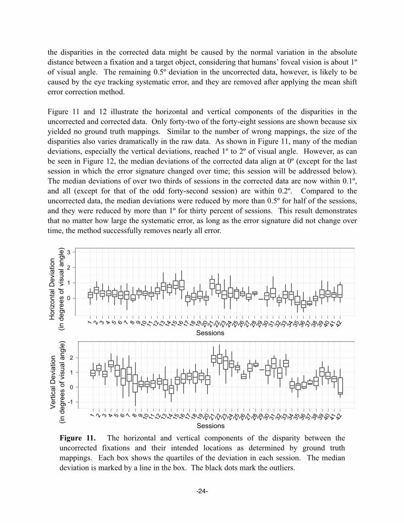
the disparities in the corrected data might be caused by the normal variation in the absolute distance between a fixation and a target object, considering that humans’ foveal vision is about 1º of visual angle. The remaining 0.5º deviation in the uncorrected data, however, is likely to be caused by the eye tracking systematic error, and they are removed after applying the mean shift error correction method.

Figure 11 and 12 illustrate the horizontal and vertical components of the disparities in the uncorrected and corrected data. Only forty-two of the forty-eight sessions are shown because six yielded no ground truth mappings. Similar to the number of wrong mappings, the size of the disparities also varies dramatically in the raw data. As shown in Figure 11, many of the median deviations, especially the vertical deviations, reached 1º to 2º of visual angle. However, as can be seen in Figure 12, the median deviations of the corrected data align at 0º (except for the last session in which the error signature changed over time; this session will be addressed below). The median deviations of over two thirds of sessions in the corrected data are now within 0.1º, and all (except for that of the odd forty-second session) are within 0.2º. Compared to the uncorrected data, the median deviations were reduced by more than 0.5º for half of the sessions, and they were reduced by more than 1º for thirty percent of sessions. This result demonstrates that no matter how large the systematic error, as long as the error signature did not change over time, the method successfully removes nearly all error.

Sessions

Ho

rizo

nta

l D

evia

tio

n

(in

de

gre

es o

f vis

ua

l a

ng

le)

0

1

2

3

1 2 3 4 5 6 7 8 9101112131415161718192021222324252627282930313233343536373839404142

Sessions

Vert

ical D

evia

tion

(in d

egre

es o

f vis

ual angle

)

-1

0

1

2

1 2 3 4 5 6 7 8 9101112131415161718192021222324252627282930313233343536373839404142

Figure 11. The horizontal and vertical components of the disparity between the uncorrected fixations and their intended locations as determined by ground truth mappings. Each box shows the quartiles of the deviation in each session. The median deviation is marked by a line in the box. The black dots mark the outliers.

-24-

Sessions

Horizonta

l D

evia

tion

(in d

egre

es o

f vis

ual angle

)

-1.0

-0.5

0.0

0.5

1.0

1.5

2.0

2.5

1 2 3 4 5 6 7 8 9101112131415161718192021222324252627282930313233343536373839404142

Sessions

Ve

rtic

al D

evia

tio

n

(in

de

gre

es o

f vis

ua

l a

ng

le)

-2

-1

0

1

1 2 3 4 5 6 7 8 9101112131415161718192021222324252627282930313233343536373839404142

Figure 12. The horizontal and vertical components of the disparity between the error-corrected fixations and their intended locations as determined by ground truth mappings.

The ground truth mappings are also compared against the mappings that were generated by applying the nearest-object fixation-assignment method to the uncorrected and corrected data set, and the result shows that the mappings from the corrected data set are more accurate. Specifically, for the uncorrected data, 97% of the fixations in the ground truth mappings were assigned to their intended targets. Whereas for the data after error correction, the percentage of correct mappings increased to 99.4%. Thus, for the fixations of the ground truth mappings, the error correction brought 2.4% accuracy improvement in terms of fixation assignments. Note that in this experiment, the accuracy of the uncorrected data seems already high. This is partly due to the effort in the instrument setup to keep the systematic error as small as possible. It is also because the distance between the visual stimuli was kept relatively large (2º in the blips’ start positions), which makes this experiment more resistant to small systematic error (less than 1º). Such design details might not be feasible in other studies, and hence the effect of the error correction method would be greater for them.

Although there are only a few wrong mappings in this experiment (3% in the uncorrected data), post error correction is still critical for the subsequent data analysis. This is because that the number of wrong mappings varied dramatically for different sessions; and for some sessions, they account for much more than 3%. For example, 15% of the mappings are wrong for the data of one participant. This high error rate is likely to influence the data analysis for this participant.

-25-

Moreover, the difference in the number of wrong mappings for different participants might create illusory individual difference in the analysis.

Both the eye movement visualizations and the quantitative measures confirm the effectiveness of the error correction method. When the error signature stay constant within a session, the method works effectively and reduces the systematic error down to nearly 0º. In the following section, we show how to extend the method to incorporate dynamic error signatures.

Possible ExtensionsThis section presents two possible ways to extend the error correction method to handle situations in which systematic error can change (a) over time and (b) across regions. Each extension is applied as follows: (1) Run the core error correction procedure for all fixations to remove the majority of the systematic error; (2) group fixations based on time or regions; and (3) apply the error correction method again for each group. It is necessary to first run the core method because it will remove a large part of the systematic error which will allow the extension to start with a better set of initial mappings.

Error Signatures Over Time

A key step for removing systematic error that changes over time is to identify at what point in time the error signature changed. One way is to go through eye movement visualizations such as shown in Figure 9 and 10 to check whether all corrected fixation locations are believable. For instance, we used VizFix to examine the problematic session (P20, Day 3, Session 2) and found that the distance between corrected fixations and possible targets increased for the first three waves of that session. Examining eye movement visualizations is an effective way for researchers to directly see the patterns of the data, but it can be time-consuming when the data set is very large. One challenge of analyzing eye movement data is to develop visualization and analysis techniques so that such trends can be found quickly and easily.

Figure 13(a) shows a variant of the disparity graph that can be used to identify the shifting of the error signature over time. The figure incorporates the temporal order of the disparities shown in the disparity plot alongside in Figure 13(b). As can be seen, after applying the initial error correction method for all fixations, most of the disparities are now centered at (0, 0). That is, most of the fixations are now within 1º to their intended targets. Some disparities are relatively far from the cluster, such as those below y = –100. From Figure 13(b), it is difficult to determine whether the disparities below y = –100 correspond to another error signature or they merely come from incorrect mappings. However, from Figure 13(a), we can see that these disparities are adjacent to each other not only in space, but also in time. If they are from incorrect mappings, they would occur randomly from time to time instead of all happening within a short time period. Thus, they are more likely to be caused by a different error signature for a short span of time.

-26-

After identifying the point in time at which systematic error changed, the fixations can be divided by the time-shift points, and the error correction procedure can be applied again for each group of fixations independently. For instance, from Figure 13(a), we found that the systematic error changed around 90 seconds after the session started. Thus, the fixations are divided into two groups at the 90 seconds mark. Figure 14 shows the disparities of the two groups, before adjusting based on time. For the first group (Figure 14, top panel), the mean shift algorithm found the error signature to be –0.95 pixels horizontal and –108.06 pixels vertical; for the second group, the error signature is 0.85 pixels horizontal and 5.77 pixels vertical. After applying the two error signatures, the median disparities of the ground truth mappings in that session changed from 5.71 to 6.66 pixels in horizontal direction, and from -106.39 to -1.95 pixels in vertical direction. This fixes the odd Session 42 box plot in Figure 12, and the error correction now works for all forty-eight sessions.


y d

evia

tio

n (

pix

els

)

-100

-50

0

50

-50 0 50 100


y d

evia

tio

n (

pix

els

)

-100

-50

0

50

-50 0 50 100

(a) (b)Figure 13. Horizontal and vertical disparity between each recorded fixation location and the closet target after applying the initial error correction for all fixations of P20, Day 3, Session 2. Graph (a) adds additional temporal orderings to the disparities shown in graph (b). Each line segment connects a pair of successive disparities. Color denotes the time the fixation occurred, with time moving from blue to red. Forty pixels is equal to 1º of visual angle.

-27-

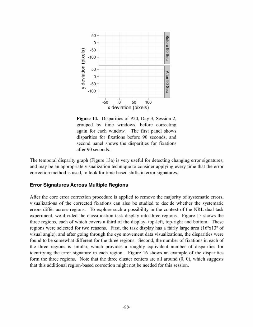
The temporal disparity graph (Figure 13a) is very useful for detecting changing error signatures, and may be an appropriate visualization technique to consider applying every time that the error correction method is used, to look for time-based shifts in error signatures.

Error Signatures Across Multiple Regions

After the core error correction procedure is applied to remove the majority of systematic errors, visualizations of the corrected fixations can also be studied to decide whether the systematic errors differ across regions. To explore such a possibility in the context of the NRL dual task experiment, we divided the classification task display into three regions. Figure 15 shows the three regions, each of which covers a third of the display: top-left, top-right and bottom. These regions were selected for two reasons. First, the task display has a fairly large area (16ºx13º of visual angle), and after going through the eye movement data visualizations, the disparities were found to be somewhat different for the three regions. Second, the number of fixations in each of the three regions is similar, which provides a roughly equivalent number of disparities for identifying the error signature in each region. Figure 16 shows an example of the disparities form the three regions. Note that the three cluster centers are all around (0, 0), which suggests that this additional region-based correction might not be needed for this session.

Figure 14. Disparities of P20, Day 3, Session 2, grouped by time windows, before correcting again for each window. The first panel shows disparities for fixations before 90 seconds, and second panel shows the disparities for fixations after 90 seconds.


y d

evia

tion (

pix

els

)

-100

-50

0

50

-100

-50

0

50

-50 0 50 100

Befo

re 9

0 S

ec

Afte

r 90 S

ec

-28-

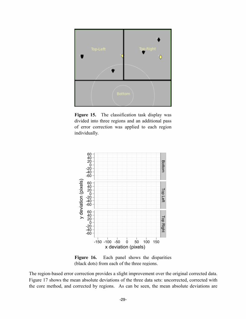
The region-based error correction provides a slight improvement over the original corrected data. Figure 17 shows the mean absolute deviations of the three data sets: uncorrected, corrected with the core method, and corrected by regions. As can be seen, the mean absolute deviations are

Figure 15. The classification task display was divided into three regions and an additional pass of error correction was applied to each region individually.

Figure 16. Each panel shows the disparities (black dots) from each of the three regions.


y d

evia

tio

n (

pix

els

)

-60

-40

-20

0

20

40

60

-60

-40

-20

0

20

40

60

-60

-40

-20

0

20

40

60

-150 -100 -50 0 50 100 150

Bottom

To

p L

eft

Top

Rig

ht

-29-

generally large in the uncorrected data. For the two corrected data sets, the mean absolute deviations and their variations are much smaller, but there is not much difference between them. The measure—the number of correct mappings—shows that the error correction by region provides no accuracy improvement; the additional correction identifies only one new correct mapping, and seven previously correct fixations were lost. The fixation loss happened because eye movement shifts across the region boundaries separated gaze points that initially comprised fixations at the region boundaries. Considering that the correction by regions did not provide much improvement in accuracy, for this experiment it is better to just use the initial error correction with the extension of error signatures that change over time.

In summary, the error correction method presented here can reliably identify the true error signature for experiments with or without moving objects, and it can also be extended to find the changing error signatures across different screen regions or different time windows. The core error correction method, in which only a single error signature was applied to the whole display, works sufficiently well. In order to clean up systematic error that changes over time, researchers can visually examine the temporal disparity graph to look for a shifting point of the error signature. For the NRL dual task experiment data, there seems to be little benefit by doing an additional pass of error correction for subregions, but it might be needed for larger displays.

Unlike Hornof and Halverson’s RFL technique, the core error correction method presented here applies a single error vector across the whole display. This single-vector approach might be less accurate considering that systematic error can vary across different areas. However, it is difficult to obtain multiple error vectors that cover many regions in an experiment with stimuli that appear at non-fixed locations. Also, the method presented here provides a way to the fixations to

Me

an

Ab

so

lute

De

via

tio

n

(de

gre

es o

f vis

ua

l a

ng

le)

0.5

1.0

1.5

2.0

uncorrected corrected corrected for

multiple regions

Figure 17. The range of mean absolution deviation for each session in different data sets.

-30-

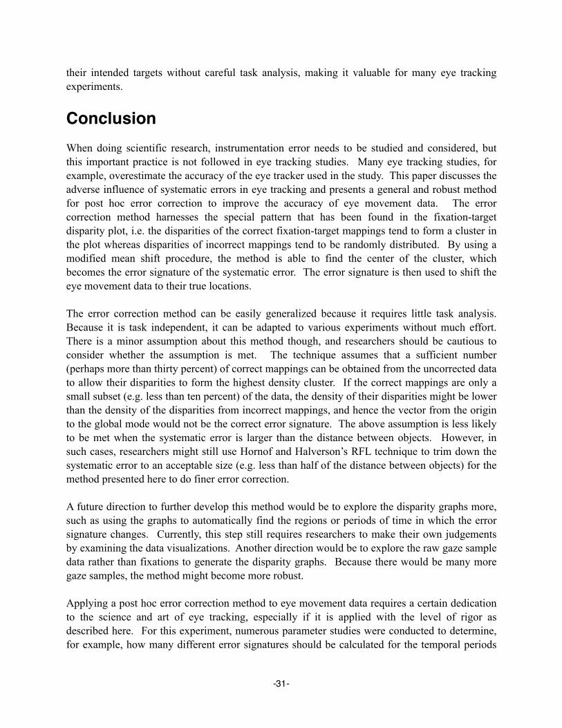
their intended targets without careful task analysis, making it valuable for many eye tracking experiments.

ConclusionWhen doing scientific research, instrumentation error needs to be studied and considered, but this important practice is not followed in eye tracking studies. Many eye tracking studies, for example, overestimate the accuracy of the eye tracker used in the study. This paper discusses the adverse influence of systematic errors in eye tracking and presents a general and robust method for post hoc error correction to improve the accuracy of eye movement data. The error correction method harnesses the special pattern that has been found in the fixation-target disparity plot, i.e. the disparities of the correct fixation-target mappings tend to form a cluster in the plot whereas disparities of incorrect mappings tend to be randomly distributed. By using a modified mean shift procedure, the method is able to find the center of the cluster, which becomes the error signature of the systematic error. The error signature is then used to shift the eye movement data to their true locations.

The error correction method can be easily generalized because it requires little task analysis. Because it is task independent, it can be adapted to various experiments without much effort. There is a minor assumption about this method though, and researchers should be cautious to consider whether the assumption is met. The technique assumes that a sufficient number (perhaps more than thirty percent) of correct mappings can be obtained from the uncorrected data to allow their disparities to form the highest density cluster. If the correct mappings are only a small subset (e.g. less than ten percent) of the data, the density of their disparities might be lower than the density of the disparities from incorrect mappings, and hence the vector from the origin to the global mode would not be the correct error signature. The above assumption is less likely to be met when the systematic error is larger than the distance between objects. However, in such cases, researchers might still use Hornof and Halverson’s RFL technique to trim down the systematic error to an acceptable size (e.g. less than half of the distance between objects) for the method presented here to do finer error correction.

A future direction to further develop this method would be to explore the disparity graphs more, such as using the graphs to automatically find the regions or periods of time in which the error signature changes. Currently, this step still requires researchers to make their own judgements by examining the data visualizations. Another direction would be to explore the raw gaze sample data rather than fixations to generate the disparity graphs. Because there would be many more gaze samples, the method might become more robust.

Applying a post hoc error correction method to eye movement data requires a certain dedication to the science and art of eye tracking, especially if it is applied with the level of rigor as described here. For this experiment, numerous parameter studies were conducted to determine, for example, how many different error signatures should be calculated for the temporal periods

-31-

of an eight-minute task and for different spatial regions of the display. It is much easier to simply report the eye tracker accuracy reported by the manufacturer, and from then on to ignore any possible error in the eye tracking data or, if error happens to be noticed in some trials, to just discard those trials. However, we believe that a bold, daring, and honest look at eye movement data and a commitment to attacking error is critical for the advancement of eye tracking research and application.

BibliographyAbrams, R. A. & Jonides, J. (1988). Programming saccadic eye movements. Journal of Experimental Psychology: Human Perception and Performance, 14(3), 428-443.

Blignaut, P. J., Beelders, T. R., & So, C. Y. (2008). The visual span of chess players. In Proceedings of the Eye Tracking Research and Applications Symposium (pp. 165-171). New York: ACM Press.

Burke, M., Hornof, A., Nilsen, E., & Gorman, N. (2005). High-cost banner blindness: Ads increase perceived workload, hinder visual search, and are forgotten. ACM Transactions on Computer-Human Interaction (TOCHI), 12(4), 445.

Comaniciu, D. & Meer, P. (2002). Mean shift: A robust approach toward feature space analysis. IEEE Transactions on Pattern Analysis and Machine Intelligence, 24(5), 603-619.

Ericcson, K. A. & Simon, H. A. (1980). Verbal reports as data. Psychological Review, 87(3), 215-251.

Findlay, J. M. & Gilchrist, I. D. (2003). Active Vision: The Psychology of Looking and Seeing. New York: Oxford University Press.

Goldberg, J. H., Stimson, M. J., Lewenstein, M., Scott, N., & Wichansky, A. M. (2002). Eye tracking in web search tasks: Design implications. In Eye Tracking Research and Applications Symposium (pp. 55-58).

Hornof, A. J. & Halverson, T. (2002). Cleaning up systematic error in eye-tracking data by using required fixation locations. Behavior Research Methods Instruments and Computers, 34(4), 592-604.

Hornof, A. J., Zhang, Y., & Halverson, T. (2010). Knowing where and when to look in a time-critical multimodal dual task. In Proceedings of CHI ’10: ACM Conference on Human Factors in Computing Systems. New York: ACM.

Hornof, A. J. & Zhang, Y. (2010, to appear). Task-constrained interleaving of perceptual and motor processes in a time-critical dual task as revealed through eye tracking. To appear in Proceedings of ICCM 2010: International Conference on Cognitive Modeling, 6 pages.

Jacob, R. J. & Karn, K. S. (2003). Eye tracking in human-computer interaction and usability research: Ready to deliver the promises. In The Mind's Eyes: Cognitive and Applied Aspects of Eye Movements. (pp. 573-605). North-Holland.

-32-

Juhasz, B. J., Liversedge, S. P., White, S. J., & Rayner, K. (2006). Binocular coordination of the eyes during reading: Word frequency and case alternation affect fixation duration but not fixation disparity. Quarterly Journal of Experimental Psychology, 59(9), 1614–1625.

Karsh, R. & Breitenbach, F. W. (1983). Looking at looking: The amorphous fixation measure. In R. Groner, C. Menz, D. F. Fisher, & R. A. Monty (Eds.), Eye Movements and Psychological Functions: International Views. (pp. 53-64). Hillsdale, NJ: Erlbaum.

Kieras, D. E., & Meyer, D. E. (1997). An overview of the EPIC architecture for cognition and performance with application to human-computer interaction. Human-Computer Interaction, 12(4), 391.

LC Technologies (2000). The Eyegaze Development System: A Tool For Eyetracking Applications.

Mello-Thoms, C., Nodine, C. F., & Kundel, H. L. (2002). What attracts the eye to the location of missed and reported breast cancers? In Proceedings of the Eye Tracking Research and Applications Symposium (pp. 111-117).

Li, D., Babcock, J., & Parkhurst, D. J. (2006). OpenEyes: A low-cost head-mounted eye-tracking solution. In Proceedings of the Eye Tracking Research and Applications Symposium (pp. 95-100).

Newell, A. & Simon, H. A. (1972). Human Problem Solving. Prentice-Hall Englewood Cliffs, NJ.

Newell, A. (1990). Unified theory of cognition. In Unified Theory of Cognition. Harvard University Press.

Salvucci, D. D. & Anderson, J. R. (2001). Automated eye-movement protocol analysis. Human-Computer Interaction, 16(1), 39-86.

Salvucci, D. D. & Goldberg, J. H. (2000). Identifying fixations and saccades in eye-tracking protocols. In Proceedings of the Eye Tracking Research and Applications Symposium (pp. 71-78).

Shen, C., Brooks, M. J., & Van Den Hengel, A. (2007). Fast global kernel density mode seeking: Applications to localization and tracking. IEEE Transactions on Image Processing, 16(5), 1457.

Smith, B. A., Ho, J., Ark, W., & Zhai, S. (2000). Hand eye coordination patterns in target selection. In Proceedings of the Eye Tracking Research and Applications Symposium (pp. 117-122).

-33-

AppendixGround Truth Mapping Rules

The following constraints were applied to identify the “ground truth” blips that participant directly fixated. These mappings were used to evaluate the eye movement data accuracy after error correction.1. Only eye movement data from the last day were used. Because on the last day, participants

acquired expert strategies for doing the dual task, the performance were more stable and predictable.

2. Only trials with more than 98% valid eye movement data rate were used. Losing more than 2% eye movement data would bring uncertainty to the process of finding ground truth mappings.

3. The associated blip must have been correctly classified. If a blip was correctly classified, there should be at least one fixation on the blip to get its ID number.

4. During the time of the fixation, there should be only one active blip (ready to be classified) on the classification task display. Two or more active blips might compete for visual attention, hence bringing uncertainty.

5. The fixation following the fixation should be on the tactical task display. This is a strategy that all participants adopted. Immediately after perceiving an active blip, they return back to the tracking task and then key in the classification. We use this rule to avoid undershoot and overshoot fixations because after such fixations, there is generally another fixation on the target blip as opposed to on the tracking task display.

6. The fixation should be the longest fixation on the classification display during its associated blip’s active time. This is because that the longest fixation was almost certainly perceiving a blip’s classification.

7. The distance between the fixation and its associated blip should be no more than 4º of visual angle.

-34-

Documents

Using the Mean Shift Algorithm to Make Post Hoc