Using the AHS to Explore Job Change, Commuting, and Salary

–An Investigative Extension

The Dean’s Research Seminar Series

March 16, 2007

General Discussion Outline

• Purpose

• Literature, Research

• The American Housing Survey

• Current Effort (Exploratory Extension)

• Analysis, Results

• Comments, Limitations

• Conclusions

The Initial Article

• Impact of Moving and Job Changes on Commuting Time– Econometrica, Inc. (Eggers & Moumen),

January 2005• “Published” at http://www.huduser.org/

– Contracted by HUD to study relationship between moving, job changes, and commuting time

– Question of what the AHS can be used for when specific questions are not asked

The Initial Article

• Had to distinguish between different household members and relationships– “Members commute, households do not”

• Problems– AHS is concerned with the housing unit; the

people are secondary– Data is not collected on location of

employment

Current Research Purpose

• Exploratory Effort– Intention is to inform current research on the

AHS national dataset– Examine how salary is related to job change,

distance, and time commuted– Use regression analysis to look at SES

and other factors– Evaluate if the Econometrica article had merit

(specifically, the proxy value)

Current Research Purpose

• Continues past and current work with the AHS– Chapman, et al (2003). Presentation at 2003

Urban Affairs Association Conference (Washington, DC).

– Chapman& Lombard (2006). Determinants of Neighborhood Satisfaction in Fee-Based Gated and Nongated Communities. Urban Affairs Review, 41(6), 769-799.

– Chapman, et al. Dissertation-in-progress (Defended and Defensible Neighborhoods).

Selected Literature

• White (1986) - Men tended to have longer commute lengths. Women had a significant positive result with the presence of young children in the house. Male homeowners tended to have longer commute lengths than renters, but there was no significant difference between female owners and renters. For both genders, blacks had a larger commuting length.

• Shen (2000) indicated that commute time is generally longer for central city low-income, lower educated minorities, primarily due to reliance on public transportation. Shen also found a gender factor, where females have a shorter commute.

• Dubin (1991) - commuting time is more important to workers than commuting distance, in relation to their decisions on employment decentralization

Selected Literature

• Clark, Huang, and Withers (2003) - households with large distances between employment location and home tend to make changes to decrease the time and distance. Males are less likely to minimize commuting after a move and females commute shorter distances.

• Ory, et al, (2004) were not persuaded that the traditional view of commuting was true for every individual, as some economic models may suggest. Two commuters who travel the same amount each week might view the amount differently. Some commuters may appreciate the private time in their vehicle, enjoy traveling, and/or find the drive somehow productive.

…thus, we have a mixed bag.

The Working Dataset

Let’s take a look at what the American Housing Survey is…

American Housing SurveyA Brief Introduction

• National and Metropolitan version• Collected biannually by U. S. Census

Bureau for the U.S. Department of Housing and Urban Development

• Housing Unit is the basis for all cases• Longitudinal components• More than 55,000 housing units surveyed

(many different types of housing units)• More than 100,000 individuals in

those housing units

American Housing SurveyA Brief Introduction

• Relational dataset (eight tables)• Over 800 variables (columns)• SAS data – can be converted to SPSS,

Stata, etc.• Contains “weight” variables for descriptive

analysis• Non-weighted dataset is “close” and

recommended by HUD for actual usage• Many different housing situations to

research

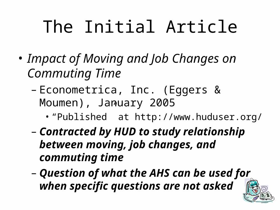
American Housing SurveyA Brief Introduction

American Housing SurveyA Brief Introduction

• How to make sense of it?– Newhouse file

• Housing unit• Respondent

– File flattening programs (SAS)

• Flattens relational structure

• Individuals 1-16• Downsides:

– No inherent or assumed order of individuals

– Huge dataset

Control # a …

Control # b …

… …

Control # xyzm …

Case 1 …

Case 2 …

… …

Case n …

Control # a … … …

Control # b … … …

… … … …

Control # xyzm … … …

Control # a …

Control # b …

… …

Control # xyzm …

Control # a …

Control # b …

… …

Control # xyzm …

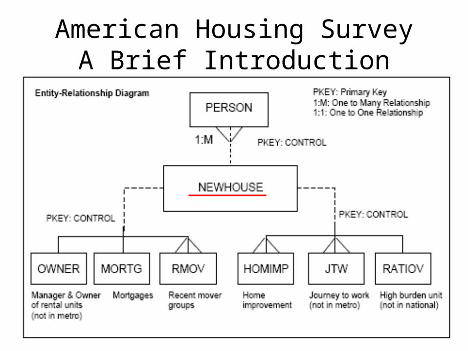
The Suggested Proxy

• How?– Econometrica used a

change in the reported distance (miles) to work as a proxy for job change

– Linked two years of data (1999 and 2001) by Control variable for housing unit

X

-X+X

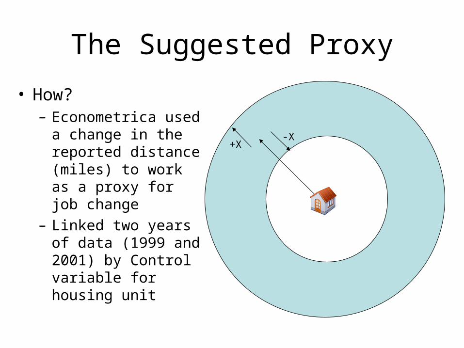
The Proxy

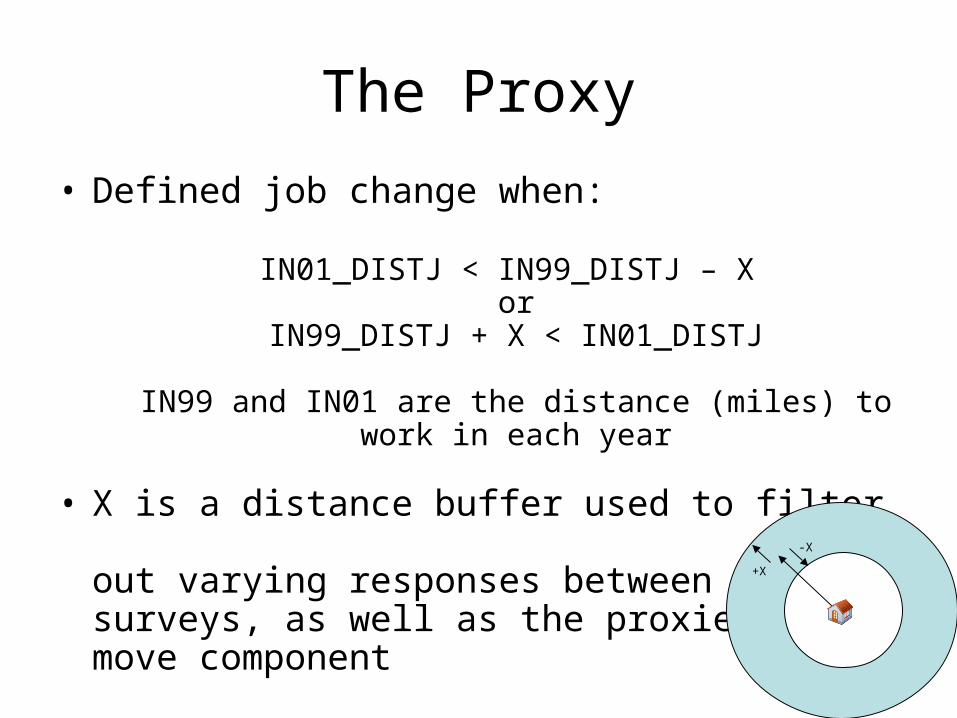
• Defined job change when:

IN01_DISTJ < IN99_DISTJ – X or

IN99_DISTJ + X < IN01_DISTJ

IN99 and IN01 are the distance (miles) to work in each year

• X is a distance buffer used to filter out varying responses betweensurveys, as well as the proxiedmove component

X

-X

+X

The Proxy

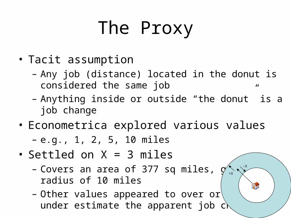
• Tacit assumption– Any job (distance) located in the donut is considered the

same job– Anything inside or outside “the donut” is a job change

• Econometrica explored various values– e.g., 1, 2, 5, 10 miles

• Settled on X = 3 miles– Covers an area of 377 sq miles, given a

radius of 10 miles– Other values appeared to over or

under estimate the apparent job change

X

-X

+X

Conclusions of Econometrica Study

• Type of household appears related to decision to move, change jobs, and commuting changes

• “Movers” have shortest current commuting distance

• “Stayers” who change jobs have the longest commute distances

• Relationship between job change and commuting time seems to depend on type of household

• Suggest that HUD and Census add a simple question about job change since last survey

Econometrica Study

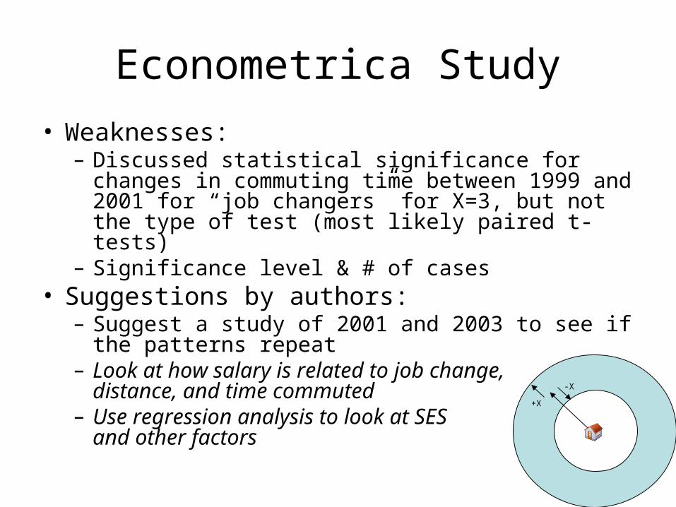
• Weaknesses:– Discussed statistical significance for changes in

commuting time between 1999 and 2001 for “job changers” for X=3, but not the type of test (most likely paired t-tests)

– Significance level & # of cases• Suggestions by authors:

– Suggest a study of 2001 and 2003 to see if the patterns repeat

– Look at how salary is related to job change, distance, and time commuted

– Use regression analysis to look at SES and other factors X

-X

+X

Extension of the Econometrica Study Using the AHS

• AHS (National)– 2005, 2003

• Look at housing units across the more current period• Merge data, order vertically/horizontally, and examine lagged

values

• Restrictions– Narrow the range of housing

unit types– Commuting time of day– Age Range (25-65 in 2005)– Salary Range ($20K-100K

in 2003 and 2005)

X

-X

+X

Extension of the Econometrica Study Using the AHS

• Restrictions– Households who worked for a salary and

commuted (distance > 0, time > 0)– Eliminate “super” commuters

(distance > 100 miles or time > 120 minutes )– Owners/renters– People who live in

“standard” housing

X

-X

+X

Note: cannot look at tenure and housing value simultaneously

Extension of the Econometrica Study Using the AHS

• Used suggested proxy of original study– Created nominal categories for year

groupings– Looked at two groups

• Single salary• Multi-salary (preliminary)

– Higher salary as primary

• Checked for inconsistencies– Year checks, cross checks– Anomalies, others…

X

-X

+X

Descriptives – One Salary Household

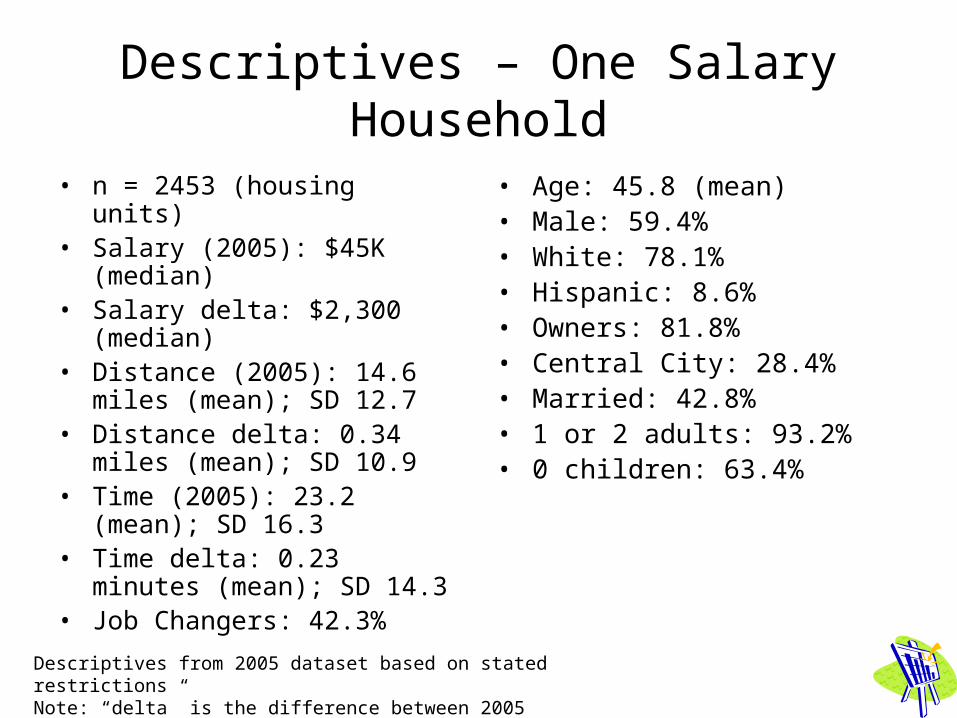
• n = 2453 (housing units)• Salary (2005): $45K (median)• Salary delta: $2,300 (median)• Distance (2005): 14.6 miles

(mean); SD 12.7• Distance delta: 0.34 miles

(mean); SD 10.9• Time (2005): 23.2 (mean); SD

16.3• Time delta: 0.23 minutes

(mean); SD 14.3• Job Changers: 42.3%

• Age: 45.8 (mean)• Male: 59.4%• White: 78.1%• Hispanic: 8.6%• Owners: 81.8%• Central City: 28.4%• Married: 42.8%• 1 or 2 adults: 93.2%• 0 children: 63.4%

Descriptives from 2005 dataset based on stated restrictionsNote: “delta” is the difference between 2005 and 2003 data

Let’s Look at Two Models

• Job Changer (y/n), using one survey year

• Job Changer (y/n) with commuting distance & time and salary deltas (2005-2003)

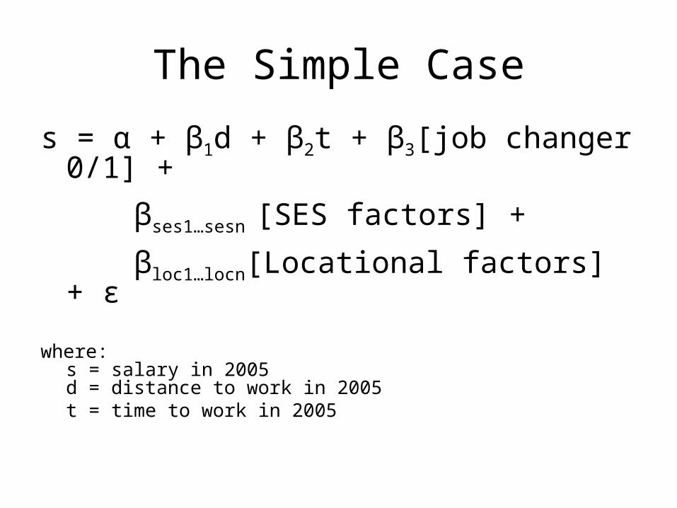
The Simple Case

s = α + β1d + β2t + β3[job changer 0/1] +

βses1…sesn [SES factors] +

βloc1…locn[Locational factors] + ε

where:s = salary in 2005d = distance to work in 2005 t = time to work in 2005

The Simple CaseResults – One Salary Household

• OLS– α < .01

• Significant results– Female (-)– Black or Hispanic (-)– Renter (-)– Not married (-)– Education (+)– 2+ adults (-)– Outside of MSA (urban

or rural) (-)

• Not significant– Job Change Construct– Commute Distance– Commute time– Others (age, presence

of children)

• Adjusted R2 = .253

The Delta Model

Δs = α + β1Δ d + β1Δ t +

β1 [job changer 0/1] +

βses1…sesn [SES factors] +

βloc1…locn [Locational factors] + ε

where:Δ s = difference in salary (2005-2003)Δ d = difference in distance (2005-2003)Δ t = difference in time (2005-2003)

The Delta ModelResults – One Salary Household

• OLS– α < .01

• Significant results– Age (-)– Female (-)– Education (grad

degree) (+)– 3+ adults (-)

• Not significant– Job Change Construct– Commute Time delta– Commute Distance

delta– Others (ethnicity,

home ownership, marital status, area)

• Adjusted R2 = .023 (!)

Multi-Salary Households

• Performed preliminary investigations• Problems with outliers and residuals• Many combinations of household types• No great improvements or hint of anything

there

Comments

• “So What?”– The significant results in the one-person case barely

look like a generalized study on salary and not much else

– The multi-person cases do not appear to be any better one-person cases

– The proxy value did not appear to add value (of any sort)

– Undoubtedly, other IVs could be explored

• May be a problem of cross-year comparisons within the AHS

• AHS may be “the wrong wine for the meal”

Limitations

• Original article was asking questions not directly answered by the AHS survey– Data derivation is daunting

• Original study was basically descriptive• Tremendous combinations of housing unit types• Censored cases• No clear order in the dataset of “importance” in the

household• Many additional exclusions and data checking are possible

– Clearly violates any sense of “Occam's razor”• Uncovered inconsistencies in the AHS

– Some were already known to us– May have discovered additional survey bias (e.g.,

non-sampled housing units between survey years could be SES driven)

Next Steps

• Investigate finer levels of the construct of job change (0, 1, 2, ...)

• Investigate further survey bias along SES dimensions

• Investigate commute distance and time deltas

Conclusions

• AHS has tremendous width/breadth, but…– The suggestion of a proxy distance to suggest job

change may be a stretch– Indirect answers are difficult and laborious to cull– The problem may be compounded when looking

across survey years– The information may be in the dataset, but may

require too many resources (or other tools) to dig out

• Use the right tool for the job