Using Solver PDF

12

Using SolverExcel has two tools, Goal Seek and Solver, that can save a greatdeal of time with complex mathematics. From a practical point ofview the simple tool Goal Seek is redundant. It has limited scopeand is far outpaced by Solver. So why is it there? Simply because,being easier to use, it is less intimidating for the mathematicallychallenged. So we shall spend a brief time on it.

Solver, which is leased by Microsoft from Frontline Systems Inc.,was developed primarily for solving optimization (maximum andminimum) problems. However, it can also be used to solveequations, and that is where we shall start. You may wish to visitwww.solver.com to learn more about this product and itsvariations. The site also has a tutorial for using the Excel Solver,but it concentrates on optimization problems; we will do morewith Solver.

In this chapter we will see examples where Solver is used (i) forequation solving, (ii) for curve fitting or regression analysis, and(iii) some simple optimization problems.

Solver needs to be installed on your computer and loaded intoExcel. It is likely this happened when Excel was installed. To check,open the Data tab and look in the Analysis group for a Solver icon.Ifyou do not see it, use the Excel Help with the search word solverto get instructions on loading it. The Excel Help has nothing moreabout Solver, as Solver has its own Help facility.

Exercise 1: Goal Seek Suppose you have an equation such as Exp(-x) - Sin(x) = aandyou know (perhaps from making a simple plot) that this has aroot such that a<=x <=1. You could set up a worksheet similarto Figure 12.1 (please ignore the Goal Seek dialogs for now),and by altering the value in AS and watching BSyou could findwhatvalue ofx makes the function zero. Think for a moment ofwhat strategy you would adopt. You could confirm that therewas a root within (0,1) by making AS first a then 1 andobserving that f(x) changes sign. Next, you might next try themidpoint O.S and then 0.6. As the sign and magnitude of BSchange, you would modify the direction and amount by which

212 A Guide to Microsoft Excel 2007for Scientists and Engineers

you altered AS until BS was nearly a-or you got tired of thegame ! Well, GoalSeek wo rks the same way. Let us see Goal Seekat work.

Figure 12.1(a) On Sheetl of a new workbook, enter what you see in Figure

12.1 without the text box. The formula in BS is =EXP(-A5)5IN(A5).

Note that the To Value mustbe a number; it cannot be acell reference. 50 if you wantD5 to equal D6, then you willneed a cell with =D5-D6, andthis will be your SetCellwithoas the To Value.

(b) Use the command Data / Data Tools / What-IfAnalysis to openthe Goal Seek dialog.

(c) Our formula is in B5, so this is the Set Cell. We want to makethis 0, so that is what we type in the To Value box, Thevariable is the value in A5, so this is the By Changing Cell.When these have been entered, click the OK button.

(d) GoalSeek now displays its Status dialog giving you the optionto either accept what it has found or cancel the operation.Click OK.

(e) Repeat steps (c) and (d) using different starting values (say0,1, and 0.5). Note howyouhave to reenter the problem eachtime you call up Goal Seek.

Note that the results vary slightly. Goal Seek quits when it hasmade a certain number of trials (iterations), when a certain timeperiod has passed, or when two answers are within a certainrange of each other (convergence limit). There is no way ofchanging these settings.

(f) If your starting value is 2, Goal Seek will find another root.Make a quick plot and see if you understand why.

(g) Save the workbook as Chap12.xlsx.

Exercise 2: Solver asRoot Finder

Using Solver 213

As an introduction to Solver, we will use it to solve the sameproblem as in Exercise 1.

Figure 12.2

(a) Open Sheetl of Chap12.xlsx. In AS enter the value 1.

(b) Use the command Data / Analysis / Solver to open the dialogshown in the top of Figure 12.2. You can see this is muchmore detailed than Goal Seek.

(c) For this problem: The Set Target is B5,with Value Ofselectedand set to 0, and By Changing Cells is A5. Click the Solvebutton in the top right corner.

(d) Solver finds an answer, and the Results dialog pops up. Notethat you can accept the answer or return to the originalvalues. The reports are relevant only for optimizationproblem, not for a Value Ofproblem. Click OK.

(e) SetAS to 0 and try again. Note (i) that Solver remembers theproblem and (ii) the results are more consistent.

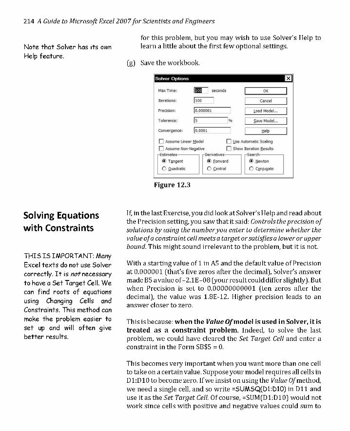
(f) Open Solver again butbefore you click Solve, open the Optionsdialog; see Figure 12.3. We shall not make any adjustments


Note that Solver has its ownHelp feature.

Solving Equationswith Constraints

THIS IS IMPORTANT: ManyExcel texts do not use Solvercorrectly. It is not necessaryto have a Set Target Cell. Wecan find roots of equationsusing Changing Cells andConstraints. This method canmake the problem easier toset up and will often givebetter results.

for this problem, but you may wish to use Solver's Help tolearn a little about the first few optional settings.

(g) Save the workbook.

Figure 12.3

If,in the last Exercise, you did look at Solver's Help and read aboutthe Precision setting, you saw that it said: Controls the precision ofsolutions by using the numberyou enter to determine whether thevalue ofa constraint cell meets a target or satisfies a lower or upperbound. This might sound irrelevant to the problem, but it is not.

With a starting value of 1 in AS and the default value of Precisionat 0.000001 (that's five zeros after the decimal), Solver's answermade B5 avalue of-2.1E-08 (your result could differ slightly). Butwhen Precision is set to 0.00000000001 (ten zeros after thedecimal), the value was 1.8E-12. Higher precision leads to ananswer closer to zero.

This is because: when the Value O[model is used in Solver, it istreated as a constraint problem. Indeed, to solve the lastproblem, we could have cleared the Set Target Cell and enter aconstraint in the Form $B$5 = O.

This becomes very important when you want more than one cellto take on a certain value. Suppose your model requires all cells inD1:D10 to become zero. Ifwe insist on using the Value afmethod,we need a single cell, and so write =SUMSQ(Dl:DlO) in Dll anduse it as the Set Target Cell. Ofcourse, =SUM(D1:D10) would notwork since cells with positive and negative values could sum to

Exercise 3: FindingMultiple Roots

Using Solver 215

zero. A far better way is to use the constraint setting ofD1:D10 =O. This is the method we use in the next exercise.

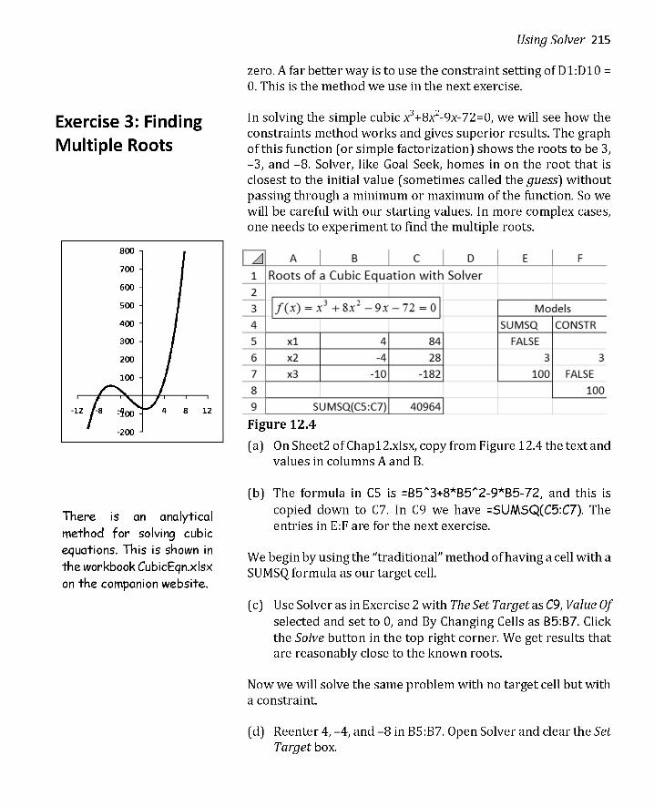
In solving the simple cubic x3+8x2-9x-72=O, we will see how theconstraints method works and gives superior results. The graphof this function (or simple factorization) shows the roots to be 3,-3, and -8. Solver, like Goal Seek, homes in on the root that isclosest to the initial value (sometimes called the guess) withoutpassing through a minimum or maximum of the function. So wewill be careful with our starting values. In more complex cases,one needs to experiment to find the multiple roots.

12

Figure 12.4

(a) On Sheet2 ofChap12.xlsx, copy from Figure 12.4 the text andvalues in columns A and B.

There is an analyticalmethod for solving cubicequations. This is shown in

the workbook CubicEqn.xlsxon the companion website.

(b) The formula in CS is =B5"'3+8*B5"'2-9*B5-72, and this iscopied down to C7. In C9 we have =SUMSQ(C5:C7). Theentries in E:F are for the next exercise.

We begin by using the "traditional" method of having a cell with aSUMSQ formula as our target cell.

(c) Use Solver as in Exercise 2 with The Set Target as C9,Value Ofselected and set to 0, and By Changing Cells as B5:B7. Clickthe Solve button in the top right corner. We get results thatare reasonably close to the known roots.

Now we will solve the same problem with no target cell but witha constraint.

(d) Reenter 4, -4, and -8 in BS:B7. Open Solver and clear the SetTarget box.

216 A Guide to Microsoft Exce/2007 for Scientists and Engineers

(e) In the Subject to Constraints area, click the Add button tobring up the Add Constraints dialog; see Figure 12.4. Enterthe constraint $C$5:$C$7 = O. You can type the rangereference with or without the $ symbols, or use the pointingmethod. Click the OKbutton. The Add button here is used toadd additional constraints.

(f) Use the Solve button to have Solver seek a solution.


The results are summarized in the table that follows.

Solver with SUMSQ cellInitial Final f(x)

4 3.0000015 9.67E-05-4 -3.0000044 0.000131

-10 -8.0000038 -0.00021

Solver with constraintsInitial Final f(x)

4 3.0000000 0-4 -3.0000000 0

-10 -8.0000000 1.73E-08

The first two Constraint results are integer values of 4 and -4; thethird value is -7.99999999968599. Clearly, the constraint methodgave superior results.

Exercise 4: SavingSolver Models

In Exercise 2 we sawthat Solver remembers the lastused settings.In Exercise 3 we had two Solver models so only the last one usedis stored. We can save information that allows us to reconstruct aSolver model.

(a) Return to Sheet2 of Chap12.xlsx and copy from Figure 12.4the text in E3:F4. The terms SUMSQ and CONSTR are usedto remind us of the features of the two models.

(b) Set Solver up to use C9as the target cell. With E5 as the activecell, open Solver's Option dialog and click on Save Model.Solver highlights a 3-by-1 range; click OK. To load the modelwe shall need to know that three cells were used to solve itSo mark these with borders/and color fills.

Exercise 5: Systems ofNonlinear Equations

Using Solver 217

(c) Set Solver up to use the constraint and no target cell. With FSas the active cell, open Solver's Option dialog and click onSave Model. Solver highlights a S-by-1 range; click OK. Markthese with borders/and color fills.

(d) Nowyou can switch from one model to the next using Options/ Load Model and selecting with appropriate block of cells.

(e) Save the workbook

In Chapter 4 we saw the use of Excel's matrix functions to solvesystems of linear equations. Figures 12.5 and 12.6 show aworksheet and Solver dialog used to solve a system of nonlinearequations. The starting values for x and y were both 1. Theanswers are not perfect; they should be integer 2 and 3, but theprecision of the method is generally acceptable for real-worldproblems.

Figure 12.5

Figure 12.6


Curve Fitting withSolver

In Chapter 7 we used various Excel functions (such as SLOPE,INTERCEPT, LINEST, and LOGEST) to fit experimental data tovarious mathematical models (linear, polynomial, exponential,etc.). We saw that the theory behind these fitting functions wasbased on the principle of minimizing the sum of the squares of theresiduals. Solver was designed to perform maximization andminimization operations, and so lends itself to curve-fittingproblems.

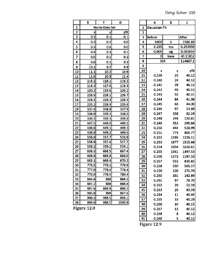
To demonstrate this method, we will do a simple linear fit withsome test data taken from the NISTwebsite (www.nist.gov). NISToffers many data sets, together with their fitting parameters toenable others to test their regression programs. We shall use theNorris data set. Figure 12.7 shows a worksheet used to fit theNorris data to y =mx + b. The Norris data set is shown in Figure12.8.

Figure 12.7

The heading s, y, and yfit in the data set were used to name thecolumns of data. Cells BS and CS were named as m and b,respectively. The formula in each cell inyfit is =mx+b. Note howExcel lets us use x to refer to just a single cell in this formula. Theformula In B3 is =SUMXMY2(y,yfit). This function convenientlygenerates the sum of the squares of the residuals. Cells B6:C6havethe formula =LINEST(y,x), while B7:C7 are copies of the valuesfrom the NISTwebsite.

With initial values of m and b as 1, the Solver model used The SetTarget is C5,with Min box selected and By Changing Cellsas B5:C5.While the LINEST results are much closer to the accepted NISTvalues, the Solver answers are quite acceptable.

E F G

1 Norris Data Set

2 x y yfit

3 0.2 0.1 -0.1

4 0.3 0.3 0.0

5 0.3 0.6 0.0

6 0.4 0.3 0.1

7 0.5 0.2 0.2

8 0.6 0.1 0.3

9 10.1 9.2 9.910 11.1 10.2 10.911 11.6 10.8 11.412 118.2 118.1 118.213 118.3 117.6 118.314 120.2 119.6 120.215 226.5 228.1 226.716 228.1 228.3 228.317 229.2 228.9 229.418 337.4 338.8 337.919 338.0 339.3 338.520 339.1 339.3 339.621 447.5 448.9 448.222 448.6 449.1 449.323 448.9 449.2 449.624 556.0 557.7 556.925 556.8 557.6 557.726 558.2 559.2 559.127 666.3 668.5 667.428 666.9 668.8 668.029 669.1 668.4 670.330 775.5 778.1 776.931 777.0 778.9 778.432 779.0 778.9 780.433 884.6 888 886.234 887.2 888 888.835 887.6 888.8 889.236 995.8 998 997.637 996.3 998.5 998.138 999.0 998.5 1000.9

Figure 12.8

Using Solver 219

A B C

1 Gaussian Fit-2

3 Before After

4 1600 h 1580.69

5 0.255 mu 0.253959

6 0.005 sig 0.003654

7 0 base 40.118528 SSR 114867.2

~10 x y yfit-11 0.239 25 40.12-12 0.240 24 40.12-13 0.241 39 40.12-14 0.242 49 40.15-15 0.243 56 40.31-16 0.244 84 41.06-17 0.245 66 44.00-18 0.246 97 53.89-19 0.247 158 82.19-

.12- 0.248 244 150.8121 0.249 353 290.84-22 0.250 444 528.99-23 0.251 773 860.77-24 0.252 1196 1226.11-25 0.253 1677 1515.68-26 0.254 1654 1620.61-27 0.255 1341 1497.53-28 0.256 1173 1197.10-29 0.257 933 830.85-

*0.258 550 505.370.259 220 275.79-

32 0.260 101 142.89-33 0.261 97 78.70-34 0.262 39 52.59-35 0.263 26 43.59-36 0.264 11 40.95-37 0.265 16 40.29-38 0.266 10 40.15-39 0.267 13 40.12-40 0.268 8 40.12-41 0.269 5 40.12

Figure 12.9


Exercise 6: GaussianCurve Fit

Having demonstrated that this is a viable method of performingregression analysis, we will use it in some more challengingexamples

Figure 12.9 shows, inA10:B41, some experimental data that is tobe fitted to a Gaussian curve. The function is given by:

( ( )2JXi - JLYi = hexp - -(J- -b

where:

Yi = the predicted valueh = the peak height above the baselineXi = the value of the independent variable

fl = the position of the maximuma = the standard deviation andb = the baseline offset

(a) On Sheet5 of Chap12.xlsx,start a worksheet similar to that inFigure 12.9. Begin by entering all the text and values exceptthe values in C4.

(b) In C4:C7 use the same values as inA4:A7. Use B4:B7 to namethe cells in C4:C7. We are going to vary the C4:C7 cells withSolver but will kept the A4:A7 values to remind us of ourstarting values.

(c) The formula in en is =h*EXP(-(((All-mu)/sig)"2))+base.There may appear to be an extra pair of parentheses in this,but that is not the case; we need to allow for the fact that thenegation operator has the highest priority.

(d) Construct a chart of the data in A10:C41. This will resemblethe chart in Figure 12.10 where the markers are they-valuesand the line the yfit-values .

You may have been wondering where the starting values for theh. tnu, and sig parameters came from. The chart will answer thisquestion. The height appears to be about 1600; the midpointseems to be in the range 0.25 and 0.26 so we use 0.255 for mu. Thestarting value for sig is found by experimentation. Try 1 in C6andsee the effect onyfit. Now try 0.5 and again see the effect onyfit.You will find that 0.005 gets yfit to more or less fitthe y-values.The tails of the curve are notfar from zero, so a starting value ofofor b would be appropriate. So now we have reasonable starting

Using Solver 221

parameters.

(e) To get ready for Solver we need a target cell holding the sumof the squares of the residuals. In C8 enter the formula=SUMXMY2(Bll:B41,Cll:C41).

(f) Use Solver to complete the task. The target cell is C8, whichwe wish to minimize by changing C4:C7. The resulting valuesare shown in Figure 12.9, while Figure 12.10 shows beforeand after fitting plots.


Before After1800

1600

1400

1200

1000

800

600

400

200

1800

1600

1400

1200

1000

800

600

400

200

0.230 0.240 0.250 0.260 0.270 0.280

Figure 12.10

0.230 0.240 0.250 0.260 0.270 0.280

Exercise 7: AMinimization Problem

Scenario: An open-top tank is to be made from a sheet of metal bybending and welding (Figure 12.11). The specifications are thatthe volume is to be 1.0 m' using the minimum sheet area. You areto find the dimensions a and b.

a

a

Figure 12.11

The worksheet to solve this problem, together with the Solverdialog, are shown in Figure 12.12.


Figure 12.12

(a) On Sheet 7 ofChap12.xlsx, enter the text shown in the figure.Enter the values in B4, BS,and HS.

(b) SelectA4:BS, then while holding! Ctrl] down, selectD4:E4 andG4:HS. Use Formula / Defined Names / Create from Selection toname the cells to the right of each text entry.

(c) Enter these formulas: in E4 =(0"'2) + (4*0*b) and in H4=0"'2*b. The parentheses in the first formula are just toimprove its readability.

(d) Set Solver up as shown in the figure and press the Solvebutton. The results should be 1.26 for a and 0.63 for b.

(e) Save the workbook.

Exercise 8: AnOptimization Problem

Sandbagger, Inc., processes sand to make semi-pure silica to sellto computer chip manufacturers at $SO/ton. The company hasPlantAand Plant B,in different locations. PlantAcan process 4S0tons/day atacostof$2S/ton, while PlantB does SSO tons/day for$20/ton.

There are three suppliers: Alpha, Beta, and Gamma. Today, Alphahas 200 tons of sand; they want $10/ton plus shipping of $2/tonto PlantAor $2.50/ton to Plant B,Beta's figures are 300 tons at$9

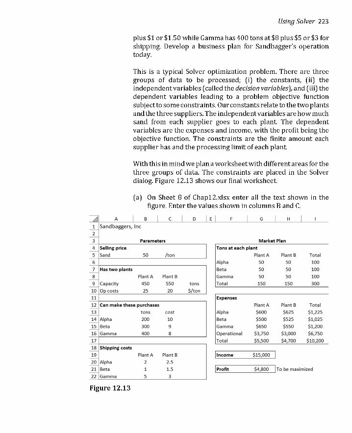
Figure 12.13

Using Solver 223

plus $1 or $1.50 while Gamma has 400 tons at $8 plus $5 or $3 forshipping. Develop a business plan for Sandbagger's operationtoday.

This is a typical Solver optimization problem. There are threegroups of data to be processed; (i) the constants, (ii) theindependentvariables (called the decision variables), and (iii) thedependent variables leading to a problem objective functionsubjectto some constraints. Our constants relate to the two plantsand the three suppliers. The independentvariables are how muchsand from each supplier goes to each plant The dependentvariables are the expenses and income, with the profit being theobjective function. The constraints are the finite amount eachsupplier has and the processing limit of each plant

With this in mind we plana worksheetwith different areas for thethree groups of data. The constraints are placed in the Solverdialog. Figure 12.13 shows our final worksheet

(a) On Sheet 8 of Chap12.xlsx enter all the text shown in thefigure. Enter the values shown in columns Band C.


(b) Enter the values of 50 into G6:H8 as our starting values forSolver to work with. These are summed in row 9 and columnI with formulas such as =5UM(G6:G8).

(c) In G13 enter =G6*($C14+B20) and copy this across and downto fill G13:H16. Sum these values in column I and row 16.Clearly, 117 gives the total of all expenses.

(d) Enter in G19 =I9*B5 (total income) and in G21 =G19-I17(profit). This last item is our objective function.

Figure 12.14

(e) All that remains is to run Solver; the settings are shown inFigure 12.14. The maximized profit comes out as $15,375using all available supplies. Save the workbook.

TK Solver" One way to test results from a computer program is to set up thesame problem in two applications. Some programmers use Excelto test results from a C# program. For the test to be valid, youmust totally rethink the problem. It is no good just programmingthe same algorithm into the second application. We want to testboth the algorithm and its implimentation in the computerapplication.

Anumber of the problems in this book have been reworked in TKSolver. For many problems, this can be a delightfully easyapplication to use: you enter rules on one sheet and variables onthe other. Then you tell TK Solver to find the unknown variable.Visitthe author's we bsite at people.stfx.cajbliengmejTKSolver tolocate the files and a link for a free trial of TK Solver. Thisapplication, which is used in many Engineering schools, can alsobe interfaced with Excel to expand its capabilities.

Problems

's. Carnahan and J. O.Wilkes, Digital Computingand Numerical Methods,Wiley, New York, 1973(page 435).

Using Solver 225

1. Download test data from www.nistgovforaGaussianfit Usethe method in Exercise 6 to fit the data. How do your valuescompare with the accepted values?

2. Redo Exercise 3 of Chapter 11 using Solver.

3. *The vapor pressure (pO in torr) ofa pure liquid as a functionof the absolute temperature can be expressed as:loglo(pO) = a - b / T. The total vapor pressure of a threecomponentmixture is given by: P = x1pt + X2P~ + X3P~ whereXi is the mole fraction of component i. Set up a worksheet touse with Solver to find the normal boiling point (thetemperature at which P = 760 torr) of a three componentmixture. For a working example, use the following data.

a b X

Benzene 7.84125 1750 0.5Toluene 8.08840 1985 0.3

Ethyl Benzene 8.11404 2129 0.2

4. *A chemical plane uses the following procedure: Avolume Vfe of solution of compound A having a concentration of 00 lbmoles/ft" is allowed to react for t, hours; the vat is thenemptied, cleaned and recharged for another cycle. It can beshown that the yield per unit time is given by:

. ld Vao(1 - exp( -ktr )yze = --"--------'--t, + t,

Make a worksheet using Solver to find the values of t, thatmaximize the yield in each simulation shown in the followingtable. Test the statement that the value of t, for maximumyield is the solution to the equation:

t, -In(trk + tk + 1) / k = 0

V 10 20 10 10 10ao 0.1 0.1 0.2 0.1 0.1k 1 1 1 0.5 1t c 0.5 0.5 0.5 0.5 1

S. *What will be the x, y-coordinates for the top right corner ofthe rectangle in the accompanying figure such that it touchesthe curve 3y = 18 - 2x 2 and the area of the rectangle ismaximized?


3y=18-2x2

Area A

0.5 1.5 2.5 3.5

2V. G. Jensen and G. V.Jeffreys, MathematicalMethods in ChemicalEngineering 2nd ed.,Academic Press, San Diego,1977, (page 570).

6. *Acompany has four sources of crude oil." Crude from eachsource can produce specific amounts of various products.Thus from column B in Figure 12.16 we see that crude Amakes 60% gasoline, 20% heating oil, and so on. Thecompany has a market for certain amounts of each product ina week (column G)and fixed supplies from each source (row10). The profit per barrel is given in row 11. How manybarrels of each type should be processed to maximize theprofit?

Figure 12.16

7. *For a change of pace, solve this magazine puzzle. Whichthree-digit number, when you divide it by the sum of itsdigits, gives you the sum of its digits plus one?

8. The Langmuir equation relates the amount of gas (5)absorbed on a surface to the pressure (p) of the gas.

S = KSrnax

l+KpFit the data in the following table to find K and Smax'

P

5

4.72

9.29

18.45

18.02

48.01

25.08

Using Solver 227

79.34 162.31 253.00

29.86 38.45 43.48

t (0e)

11 (expt)

9. InProblem 15 of Chapter 9, this equation was used to find thesurface area of a cylinder with a conical base.

2V 2( 2 )S = ---;:- + J[r esc e- "3 cot eWe can show by calculus that S is a minimum when the angleof the cone is given by 8 =cos·1(2/ 3). Use Solver to confirmthat we did the differentiation correctly. How close is Solver'svalue to the expected one? Can you improve on this?

10. Sutherland's equations can be used to derive the dynamicviscosity of an ideal gas as a function of temperature:

- Ta+C(~J%17 - 170 T +C Tawhere 11 is the viscosity (Pa-s) at temperature T, 110 is theviscosity, T is the input temperature in Kelvin, To is thereference temperature, and Cis Sutherland's constant for thespecified gas. The following table lists some measuredviscosity values for air. Given that for air, 110 = 18.27 X 10.6

Pa-s at 291.15K, find Cfor air.

10 20 30 40 50 60 70 80 90 100

17.87 18.37 18.86 19.34 19.82 20.29 20.75 21.21 21.66 22.10

11. Refer to Problem 9 in Chapter 2. Make a new worksheetbeginning with something similar Figure 12.17. Use Solver tofind the n values that maximize the profit

Figure 12.17

Do not use the UDF you may have coded in Problem 7 ofChapter 9 but compute the ml values with an Excel function.

Documents

Using Solver PDF