Using Semtex - User Web Pages - Monash University

Using Semtex

H.M. Blackburn

Monash University

October 6, 2017Semtex version 8.2

Contents

1 Introduction 31.1 Numerical method . . . . . . . . . . . . . . . . . . . . . . . . . . . . . . . . . . . . 31.2 Implementation . . . . . . . . . . . . . . . . . . . . . . . . . . . . . . . . . . . . . 41.3 Further reading . . . . . . . . . . . . . . . . . . . . . . . . . . . . . . . . . . . . . 5

2 Starting out 62.1 Testing . . . . . . . . . . . . . . . . . . . . . . . . . . . . . . . . . . . . . . . . . . 6

2.1.1 Troubleshooting installation problems . . . . . . . . . . . . . . . . . . . . . 62.2 Files . . . . . . . . . . . . . . . . . . . . . . . . . . . . . . . . . . . . . . . . . . . 72.3 Utilities . . . . . . . . . . . . . . . . . . . . . . . . . . . . . . . . . . . . . . . . . . 7

3 Examples and hints 93.1 2D Taylor flow . . . . . . . . . . . . . . . . . . . . . . . . . . . . . . . . . . . . . . 9

3.1.1 Session file . . . . . . . . . . . . . . . . . . . . . . . . . . . . . . . . . . . . 93.1.2 Running the codes . . . . . . . . . . . . . . . . . . . . . . . . . . . . . . . . 11

3.2 2D Laplace problem . . . . . . . . . . . . . . . . . . . . . . . . . . . . . . . . . . . 143.2.1 Curved element edges . . . . . . . . . . . . . . . . . . . . . . . . . . . . . . 163.2.2 Boundary conditions . . . . . . . . . . . . . . . . . . . . . . . . . . . . . . . 163.2.3 Running the codes . . . . . . . . . . . . . . . . . . . . . . . . . . . . . . . . 17

3.3 3D Kovasznay flow . . . . . . . . . . . . . . . . . . . . . . . . . . . . . . . . . . . 183.3.1 ‘High-order’ pressure boundary condition . . . . . . . . . . . . . . . . . . . . 193.3.2 Running the codes . . . . . . . . . . . . . . . . . . . . . . . . . . . . . . . . 19

3.4 Vortex breakdown—a cylindrical-coordinate problem . . . . . . . . . . . . . . . . . 203.4.1 BCs for cylindrical coordinates . . . . . . . . . . . . . . . . . . . . . . . . . 23

3.5 Boundary condition roundup . . . . . . . . . . . . . . . . . . . . . . . . . . . . . . 233.5.1 No-slip wall . . . . . . . . . . . . . . . . . . . . . . . . . . . . . . . . . . . 233.5.2 Inflow or prescribed-velocity boundary . . . . . . . . . . . . . . . . . . . . . 243.5.3 Slip (no-penetration) boundary . . . . . . . . . . . . . . . . . . . . . . . . . 243.5.4 ‘Stress-free’ outflow boundary . . . . . . . . . . . . . . . . . . . . . . . . . 243.5.5 ‘Robust’ outflow boundary . . . . . . . . . . . . . . . . . . . . . . . . . . . 243.5.6 Axis boundary . . . . . . . . . . . . . . . . . . . . . . . . . . . . . . . . . . 24

3.6 Fixing problems . . . . . . . . . . . . . . . . . . . . . . . . . . . . . . . . . . . . . 253.7 Execution speed . . . . . . . . . . . . . . . . . . . . . . . . . . . . . . . . . . . . . 25

4 Extra controls 274.1 Default values of flags and internal variables . . . . . . . . . . . . . . . . . . . . . . 274.2 Checkpointing . . . . . . . . . . . . . . . . . . . . . . . . . . . . . . . . . . . . . . 274.3 Iterative solution . . . . . . . . . . . . . . . . . . . . . . . . . . . . . . . . . . . . . 274.4 Wall fluxes . . . . . . . . . . . . . . . . . . . . . . . . . . . . . . . . . . . . . . . . 284.5 Wall tractions . . . . . . . . . . . . . . . . . . . . . . . . . . . . . . . . . . . . . . 284.6 Modal energies . . . . . . . . . . . . . . . . . . . . . . . . . . . . . . . . . . . . . . 28

1

4.7 History points . . . . . . . . . . . . . . . . . . . . . . . . . . . . . . . . . . . . . . 284.8 Averaging . . . . . . . . . . . . . . . . . . . . . . . . . . . . . . . . . . . . . . . . 294.9 Phase averaging . . . . . . . . . . . . . . . . . . . . . . . . . . . . . . . . . . . . . 294.10 Particle tracking . . . . . . . . . . . . . . . . . . . . . . . . . . . . . . . . . . . . . 294.11 Spectral vanishing viscosity . . . . . . . . . . . . . . . . . . . . . . . . . . . . . . . 304.12 General body forcing . . . . . . . . . . . . . . . . . . . . . . . . . . . . . . . . . . 30

4.12.1 Steady force . . . . . . . . . . . . . . . . . . . . . . . . . . . . . . . . . . . 314.12.2 Modulated force . . . . . . . . . . . . . . . . . . . . . . . . . . . . . . . . . 314.12.3 Sponge region . . . . . . . . . . . . . . . . . . . . . . . . . . . . . . . . . . 314.12.4 ’Drag’ force . . . . . . . . . . . . . . . . . . . . . . . . . . . . . . . . . . . 324.12.5 White noise force . . . . . . . . . . . . . . . . . . . . . . . . . . . . . . . . 324.12.6 Selective frequency damping (SFD) . . . . . . . . . . . . . . . . . . . . . . 324.12.7 Rotating frame of reference: Coriolis and centrifugal force . . . . . . . . . . 33

5 Specialised executables 345.1 Concurrent execution . . . . . . . . . . . . . . . . . . . . . . . . . . . . . . . . . . 345.2 Vector architectures . . . . . . . . . . . . . . . . . . . . . . . . . . . . . . . . . . . 34

6 Code design and the Semtex API 356.1 Useful things to know about . . . . . . . . . . . . . . . . . . . . . . . . . . . . . . 356.2 Altering the code . . . . . . . . . . . . . . . . . . . . . . . . . . . . . . . . . . . . 36

7 DNS 101 — Turbulent channel flow 387.1 Parameters . . . . . . . . . . . . . . . . . . . . . . . . . . . . . . . . . . . . . . . . 387.2 Mesh design . . . . . . . . . . . . . . . . . . . . . . . . . . . . . . . . . . . . . . . 397.3 Initiating and monitoring transition . . . . . . . . . . . . . . . . . . . . . . . . . . . 427.4 Flow statistics . . . . . . . . . . . . . . . . . . . . . . . . . . . . . . . . . . . . . . 43

2

Chapter 1

Introduction

Semtex is a family of spectral element simulation codes, most prominently a code for direct numer-ical simulation of incompressible flow. The spectral element method is a high-order finite elementtechnique that combines the geometric flexibility of finite elements with the high accuracy of spectralmethods. The method was pioneered in the mid 1980’s by Anthony Patera at MIT (Patera; 1984;Korczak and Patera; 1986). Semtex uses parametrically mapped quadrilateral elements, the classicGLL ‘nodal’ shape function basis, and continuous Galerkin projection. Algorithmically the code issimilar to Ron Henderson’s Prism (Henderson and Karniadakis; 1995; Karniadakis and Henderson;1998; Henderson; 1999), but with some differences in design, and lacks mortar element capability.A notable extension is that Semtex can solve problems in cylindrical as well as Cartesian coordinatesystems (Blackburn and Sherwin; 2004).

1.1 Numerical method

Some central features of the spectral element method are

Orthogonal polynomial-based shape functions Spectral accuracy is achieved by using tensor-product Lagrange interpolants within each element, where the nodes of these shape functionsare placed at the zeros of Legendre polynomials mapped from the canonical domain [-1, 1]×[-1, 1] to each element. In one spatial dimension, the resulting Gauss–Lobatto–Legendre La-grange interpolant which is unity at one of the N + 1 Gauss–Lobatto points xj in [-1, 1] andzero at the others is

ψj(x) =1

N(N + 1)LN (xj)

(1− x2)L′

N (x)

x− xj. (1.1)

For example, the family of sixth-order GLL Lagrange interpolants is shown in figure 1.1. Insmooth function spaces it can be shown that the resulting interpolants converge exponentially

Figure 1.1: The family of sixth-order one-dimensional GLL Lagrange shape functions on the masterdomain [−1,+1].

3

fast (faster than any negative integer power of N) as the order of the interpolant is increased.See Canuto et al. (1988), §§ 2.3.2 and 9.4.3.

Gauss–Lobatto quadrature Efficiency (particularly in iterative methods) is achieved by using Gauss–Lobatto quadrature for evaluating elemental integrals: the quadrature points reside at the nodalpoints, which enables fast tensor-product techniques to be used for iterative matrix solutionmethods. Gauss–Lobatto quadrature on the nodal points delivers diagonal mass matrices.

Static condensation Direct matrix solutions are sped up by using static condensation coupled withbandwidth reduction algorithms to reduce storage requirements for assembled system matrices.

While the numerical method is very accurate and efficient, it also has the advantage that complexgeometries can be accommodated by employing unstructured meshes. The vertices of spectralelements meshes can be produced using finite-element mesh generation procedures, or any othermethod (for Semtex, only meshes with quadrilateral elements are accepted).

Time integration employs a backwards-time differencing scheme described by Karniadakis et al.(1991), more recently classified as a velocity-correction method by Guermond and Shen (2003). Onecan select first, second, or third-order time integration, but second order is usually a reasonablecompromise, and is the default scheme. Equal-order interpolation is used for velocity and pressure(see Guermond et al.; 2006).

As of Semtex V8, the ‘alternating skew symmetric’ form (Zang; 1991) is the default for con-struction of nonlinear terms in the Navier–Stokes equations (faster and just as robust as full skewsymmetric, which is still an option), and no dealiasing of product terms is carried out for either serialor parallel operations. As an aid to robust operation at high Reynolds numbers, ‘spectral vanish-ing viscosity’ (Xu and Pasquetti; 2004) can easily be enabled by setting appropriate control tokens.A significant additional novelty of Semtex V8 is the option of robust outflow boundary conditions(Dong et al.; 2014), which alleviate much of the numerical stability problem associated with inflowsthat occur at the outflow boundary.

1.2 Implementation

The top level of the code is written in C++, with calls to C and FORTRAN library routines, e.g. BLASand LAPACK. The original implementation for two-dimensional Cartesian geometries was extendedto three dimensions using Fourier expansion functions for spatially-periodic directions in Cartesianand cylindrical spaces. Concurrent execution is supported, using MPI as the basis for interprocessorcommunications, and the code has been ported to DEC, NEC, Fujitsu, Compaq, SGI, Apple andLinux multiprocessor machines. Basically it ought to work with little trouble on any contemporaryUNIX system.

There are various code extensions that are not part of the base distribution. These include dy-namic and non-dynamic LES (Blackburn and Schmidt; 2003), simple power-law type non-Newtonianrheologies (Rudman and Blackburn; 2006), scalar transport (Blackburn; 2001, 2002a), buoyancy viathe Boussinesq approximation, accelerating frame of reference coupling for aeroelasticity (Blackburnand Henderson; 1996, 1999; Blackburn et al.; 2000; Blackburn; 2003), solution of steady-state flowsvia Newton–Raphson iteration (Blackburn; 2002b)

However, linear stability analysis (Blackburn; 2002b; Blackburn and Lopez; 2003a,b; Blackburnet al.; 2005; Sherwin and Blackburn; 2005; Elston et al.; 2006; Blackburn and Sherwin; 2007) andoptimal transient growth analysis (Blackburn et al.; 2008) are released as an additional code base(called Dog), see the accompanying user guide called ‘Working Dog ’.

4

1.3 Further reading

The most comprehensive references on spectral methods in general are Gottlieb and Orszag (1977),Canuto et al. (1988, 2006). The first papers by Patera (1984) and Korczak and Patera (1986)provide a good introduction to spectral elements, although some aspects have changed with timeand Maday and Patera (1989) is more up-to-date. The use of Fourier expansions to extend themethod to three spatial dimensions is discussed by Amon and Patera (1989), Karniadakis (1989) andKarniadakis (1990). The use of spectral element techniques in cylindrical coordinates is dealt with inBlackburn and Sherwin (2004). The book by Funaro (1997) provides useful information and furtherreferences. Recent overviews and some applications appear in Karniadakis and Henderson (1998);Henderson (1999). The definitive reference is now the book by Karniadakis and Sherwin (2005), butyou will also find the text by Deville, Fischer and Mund (2002) useful for alternative explanationsand views. More recently, the book by Canuto et al. (2007) provides both theory and applicationsof spectral as well as spectral element methods in fluid dynamics.

5

Chapter 2

Starting out

It is assumed you’re using some version of UNIX (which includes Mac OS X), and the current Semtexversions assume that your C++ compiler supports the standard libraries. Makefiles assume GNUmake(by now this is usually the standard supplied variant of make). SuperMongo and Tecplot would benice to have but are not essential to get up and running, and VTK-based post processors such as VisItor ParaView can alternatively be used for post-processing in place of Tecplot. All major executableshave a -h command line option which provides a usage prompt.

Application programs/Makefiles can be found in top and upper-level directories:

elliptic Solve elliptic (Laplace, Poisson, Helmholtz) problems.dns Solve time-varying incompressible Navier–Stokes problems, Cartesian/cylindrical.

2.1 Testing

Unpack the tar file, then run make test. This will copy header files to their correct places, compileand place the libraries, make two central utilities (compare and enumerate), then make the directnumerical simulation solver dns and run regression checks on its output for a number of test cases.If all goes well, this process will end with a number of tests reported as passed. In that case, go onand compile all the utilities, too (cd utility; make all).

2.1.1 Troubleshooting installation problems

If the above process didn’t work, there are a number of possible things lacking on your system, e.g.:

1. GNU’s make: it needs to be in your path somewhere. On most current UNIX systems, thesystem-supplied make is the GNU version. So now (as of 2010) this is assumed; you can easilycheck by running make --version and looking at the first line of output. If not, it may beinstalled as gmake. Otherwise you will need to get it installed. Alter the variable MAKE insemtex/Makefile so that it gets to the installed GNU make, if required.

2. The BLAS and LAPACK libraries— these may be in /usr/lib or /usr/local/lib: searchfor libblas and liblapack. On many systems, BLAS and LAPACK are vendor-supplied aspart of some ‘math kernel’ library. NB: since quite heavy use is made of BLAS routine dgemm,it can be worthwhile finding BLAS versions in which this is well optimised, see § 3.7.

3. A standard C++ compiler, a C compiler, and a FORTRAN compiler that can deal withFORTRAN-77. Note that F90, F95 compilers now often supplant F77 compilers, and thesecan (and should) be substituted if available. GNU’s standard FORTRAN compiler is now calledgfortran and is part of the standard gcc compiler suite.

4. Either yacc or bison.

6

If you have all these things but there are still compilation problems, you have some work to do.The first place to look is in the file src/Makefile which has the master set of compilation flags

and directives for various operating systems. You my find your system here, or one that is similar.Even if this is not the case, you should pick up some clues about how to set up for compilation ona new system. As well, check the README file in the top directory. Of course, it is possible that thecode is incompatible with some detail of your compilation system or has a bug, but it has had fairlyextensive exercise on a number of UNIX systems by now.

If you are having problems, it’s usually best to start small and work up. First try to make andinstall the veclib and femlib libraries, since they do not use C++ or the linker. Try make libs

at the top level, then if this is still problematic go to the veclib directory, do make clean; make;

make install. When that works, do the same in the femlib directory. Next move on and try asimple C++ compile and link, e.g. in the utility directory do make calc and try running calc

(which is a little like the UNIX calculator utility bc, but uses Semtex ’s function parser, and linkslibfem.a, the library produced in femlib): try say 1+1. Next you should try compiling somethingthat links to the BLAS and LAPACK, e.g. compare. Once this will compile, everything should.

2.2 Files

Semtex uses a base input file which describes the mesh, boundary conditions. We call this a sessionfile and typically it has no root extension. It is written in a format patterned on HTML, which wehave called FEML (for Finite Element Markup Language). There are a number of example sessionfiles in the mesh directory. Other files have standard extensions:

session.num Global node numbers, produced by enumerate utility.session.fld Solution/field file. Binary format by default.session.rst Restart file. Read in to initialize solution if present.session.avg Averaged results. Read back in for continuation (over-written).session.his History point data.session.flx Time series of pressure and viscous forces integrated over the wall boundary group.session.mdl Time series of kinetic energies in the Fourier modes.session.par Used to define initial particle locations.session.trk Integrated particle locations.

When writing a new session file it is best to run meshpr (and/or meshpr -c) on it before trying touse it for simulations. Meshpr will catch most of the easier-to-make errors. You can also plot up theresults using SuperMongo or other utility as a visual check.

2.3 Utilities

Source code for these is found in the utility directory. You will need to make most of these byhand (using the supplied Makefile, and make all). Here is a summary:

addfield Add vorticity vector components, divergence, etc., to a field file.calc A simple calculator that calls femlib’s function parser. The default functions

and TOKENS can be seen if you run calc -h.compare Generate restart files, compare solutions to a function.convert Convert field file formats (IEEE-big/little, ASCII).eneq Compute terms in the energy transport equation.enumerate Generate global node numbering, with RCM optimization.integral Obtain the 2D integral of fields over the domain area.interp Interpolate a field file onto a (2D) set of points.

7

meshpr Generate 2D mesh locations for plotting or checking.noiz Add a random perturbation to a field file.probe Probe a field file at a set of 2D/3D points. Different interfaces to probe

are obtained through the names probeline and probeplane:make these soft links by hand.

project Convert a field file to a different order interpolation.rectmesh Generate a template session file for a rectangular domain.resubmit Shell utility for automatic job resubmission.rstress Postprocess to compute Reynolds stresses from a file of time-averaged variables.save Shell utility for automatic job resubmission.sem2tec Convert field files to Amtec Tecplot format.

Note that by default, sem2tec interpolates the original GLL- mesh-based data ontoa (isoparametrically mapped) uniform mesh for improved visual appearance. Sometimesit is useful to see the original data (and mesh); for this use the -n 0 command-lineargument to sem2tec.

sem2vtk Convert field files to VTK format (VisIt, ParaView).transform Take Fourier, Legendre, modal basis transform of a field file. Invertible.wallmesh Extract the mesh nodes corresponding to surfaces with the wall group.

8

Chapter 3

Examples and hints

We will run through some examples to illustrate input files, utility routines, and the use of the solvers.

3.1 2D Taylor flow

Taylor flow is an analytical solution to the Navier–Stokes equations. In the x–y plane the solution is

u = − cos(πx) sin(πy) exp(−2π2νt), (3.1)

v = +sin(πx) cos(πy) exp(−2π2νt), (3.2)

p = −(cos(2πx) + cos(2πy)) exp(−4π2νt)/4. (3.3)

The solution is doubly periodic in space, with periodic length 2. As usual for Navier–Stokes solutions,the pressure can only be specified up to an arbitrary constant. An interesting feature of this solutionis that the nonlinear and pressure gradient terms balance one another, leaving a diffusive decay ofthe initial condition — this property is occasionally useful for checking codes.

3.1.1 Session file

Below is the complete input or session file we will use; it has four elements, each of the same size,with 11 nodes along each edge. We will call this session file taylor2 in the following.

##############################################################################

# 2D Taylor flow in the x--y plane has the exact solution

#

# u = -cos(PI*x)*sin(PI*y)*exp(-2.0*PI*PI*KINVIS*t)

# v = sin(PI*x)*cos(PI*y)*exp(-2.0*PI*PI*KINVIS*t)

# w = 0

# p = -0.25*(cos(2.0*PI*x)+cos(2.0*PI*y))*exp(-4.0*PI*PI*KINVIS*t)

#

# Use periodic boundaries (no BCs).

<USER>

u = -cos(PI*x)*sin(PI*y)*exp(-2.0*PI*PI*KINVIS*t)

v = sin(PI*x)*cos(PI*y)*exp(-2.0*PI*PI*KINVIS*t)

p = -0.25*(cos(TWOPI*x)+cos(TWOPI*y))*exp(-4.0*PI*PI*KINVIS*t)

</USER>

<FIELDS>

u v p

</FIELDS>

<TOKENS>

9

N_TIME = 2

N_P = 11

N_STEP = 20

D_T = 0.02

Re = 100.0

KINVIS = 1.0/Re

TOL_REL = 1e-12

</TOKENS>

<NODES NUMBER=9>

1 0.0 0.0 0.0

2 1.0 0.0 0.0

3 2.0 0.0 0.0

4 0.0 1.0 0.0

5 1.0 1.0 0.0

6 2.0 1.0 0.0

7 0.0 2.0 0.0

8 1.0 2.0 0.0

9 2.0 2.0 0.0

</NODES>

<ELEMENTS NUMBER=4>

1 <Q> 1 2 5 4 </Q>

2 <Q> 2 3 6 5 </Q>

3 <Q> 4 5 8 7 </Q>

4 <Q> 5 6 9 8 </Q>

</ELEMENTS>

<SURFACES NUMBER=4>

1 1 1 3 3 

2 2 1 4 3 

3 2 2 1 4 

4 4 2 3 4 

</SURFACES>

The first section of the file in this case contains comments; a line anywhere in the session filewhich starts with a # is considered to be a comment. Following that are a number of sections whichare opened and closed with matching keywords in HTML style (e.g. <USER>–<\USER>). Keywordsare not case sensitive. The complete list of keywords is: TOKENS, FIELDS, GROUPS, BCS, NODES,ELEMENTS, SURFACES, CURVES and USER. Depending on the problem being solved, some sectionsmay not be needed, but the minimal set is: FIELDS, NODES, ELEMENTS and SURFACES. Anywherethere is likely to be a long list of inputs within the sections, the NUMBER of inputs is also required; thiscurrently applies to GROUPS, BCS, NODES, ELEMENTS, SURFACES and CURVES. In each of these casesthe numeric tag appears first for each input, which is free-format. The order in which the sectionsappear in the session file is irrelevant.

The USER section is ignored by the solvers, and is used instead by utilities — in this case it willbe used by the compare utility both to generate the initial condition or restart file and to checkthe computed solution. This section declares the variables corresponding to the solution fields withthe corresponding analytical solutions. The variables x, y, z and t can be used to represent thethree spatial coordinates and time. Note that some constants such as PI and TWOPI are predefined,while others, like KINVIS, are set in the TOKENS section. Note also the use of predefined functions,accessed through an inbuilt function parser1.

The FIELDS section declares the one-character names of solution fields. The names are significant:u, v and w are the three velocity components (we only use u and v here for a 2D solution and the w

1The built-in functions and predefined constants can be found by running calc -h.

10

component is always the direction of Fourier expansions), p is the pressure field. The field name c

is also recognized as a scalar field for certain solvers, e.g. the elliptic solver.In the TOKENS section, second-order accurate time integration is selected (N_TIME = 2) and the

number of Lagrange knot points along the side of each element is set to 11 (N_P = 11), correspondingto the use of 10th-order polynomials, and giving two-dimensional elemental shape functions whichare tensor-products of 10th-order Lagrange polynomials.2 The code will integrate for 20 timesteps(N_STEP = 20) with a timestep of 0.02 (D_T = 0.002). The kinematic viscosity is set as the inverseof the Reynolds number (100): note the use of the function parser here. Finally the relative toleranceused as a stopping test in the PCG iteration used to solve the viscous substep on the first timestepis set as 1.0× 10−12.

The shape of the mesh is defined by the NODES and ELEMENTS sections. Here there are fourelements, each obtained by connecting the corner nodes in a counterclockwise traverse. The x, yand z locations of the nodes are given, and the four numbers given for the nodes of each elementare indices within the list of nodes.

In the final section (SURFACES), we describe how the edges of elements which define the boundaryof the solution domain are dealt with. In this example, the solution domain is periodic and there are noboundary conditions to be applied, so the SURFACES section describes only periodic (P) connectionsbetween elements. For example, on the first line, side 1 of element 1 is declared to be periodic withside 3 of element 3 — side 1 runs between the first and second nodes, while side 3 runs between thethird and fourth.

3.1.2 Running the codes

Assume we’re in the dns directory of the distribution, that the enumerate, compare, meshpr andsem2tec utilities have been compiled, as well as the dns simulation code.

karman[16] cp ../mesh/taylor2 .

First we’ll examine the mesh, using SuperMongo macros.

karman[17] meshpr taylor2 > taylor2.msh

karman[18] sm

Hello Hugh, please give me a command

: meshplot taylor2.msh 1

Read lines 1 to 1 from taylor2.msh

Read lines 2 to 485 from taylor2.msh

: meshnum

: meshbox

: quit

You should have seen a plot like that in figure 3.1. (Note: while you are building up the mesh partsof a session file, you can use meshpr -c to suppress some of the checking for matching elementedges and curved boundaries that meshpr does by default.)

Next we will generate the global numbering schemes for the solution using enumerate to producetaylor2.num. The solution code would run enumerate automatically to generate taylor2.num ifit were not present, but we will run it ‘by hand’ to highlight its existence and illustrate its use.

karman[19] enumerate taylor2 > taylor2.num

karman[20] head -20 taylor2.num

# FIELDS : uvp

# ---------------- ----------

# 1 NUMBER SETS : uvp

# NEL : 4

# NP_MAX : 11

2The minimum accepted value of N P = 2, corresponding to (bi)linear shape functions. The practicable upper valueis around 20.

11

1 2

3 4

0 0.5 1 1.5 2

0

0.5

1

1.5

2

Figure 3.1: The mesh corresponding to the taylor2 session file.

# NEXT_MAX : 40

# NINT_MAX : 81

# NTOTAL : 484

# NBOUNDARY : 160

# NGLOBAL : 76

# NSOLVE : 76

# OPTIMIZATION : 1

# BANDWIDTH : 67

# ---------------- ----------

# elmt side offst bmap mask

1 1 0 20 0

1 1 1 17 0

1 1 2 16 0

1 1 3 15 0

1 1 4 14 0

The compare utility is used to generate a file of initial conditions using information in the USERsection of a session file. This restart file contains binary data, but we’ll have a look at the start ofit by converting it to ASCII format. Also, the header of these files is always in ASCII format, and socan be examined directly using the Unix head command.

karman[21] compare taylor2 > taylor2.rst

karman[22] convert taylor2.rst | head -20

taylor2 Session

Wed Aug 13 21:39:47 1997 Created

11 11 1 4 Nr, Ns, Nz, Elements

0 Step

0 Time

0.02 Time step

0.01 Kinvis

1 Beta

uvp Fields written

ASCII Format

0.000000000 0.000000000 -0.5000000000

0.000000000 0.1034847104 -0.4946454574

12

0.000000000 0.3321033052 -0.4448536974

0.000000000 0.6310660897 -0.3008777952

0.000000000 0.8940117093 -0.1003715318

0.000000000 1.000000000 0.000000000

0.000000000 0.8940117093 -0.1003715318

0.000000000 0.6310660897 -0.3008777952

0.000000000 0.3321033052 -0.4448536974

0.000000000 0.1034847104 -0.4946454574

Then the dns solver is run to generate a solution or field file, taylor2.fld. This has the sameformat as the restart file.

karman[23] dns taylor2

-- Restarting from file: taylor2.rst

Start time : 0

Time step : 0.02

Number of steps : 20

End time : 0.4

Integration order: 2

-- Building matrices for Fields "uvp" [*]

-- Building matrices for Fields "uvp" [.]

-- Building matrices for Fields "uvp" [*]

Step: 1 Time: 0.02

Step: 2 Time: 0.04

Step: 3 Time: 0.06

Step: 4 Time: 0.08

Step: 5 Time: 0.1

Step: 6 Time: 0.12

Step: 7 Time: 0.14

Step: 8 Time: 0.16

Step: 9 Time: 0.18

Step: 10 Time: 0.2

Step: 11 Time: 0.22

Step: 12 Time: 0.24

Step: 13 Time: 0.26

Step: 14 Time: 0.28

Step: 15 Time: 0.3

Step: 16 Time: 0.32

Step: 17 Time: 0.34

Step: 18 Time: 0.36

Step: 19 Time: 0.38

Step: 20 Time: 0.4

We can use compare to examine how close the solution is to the analytical solution. The outputof compare in this case is a field file which contains the difference: since we’re only interested inseeing error norms here, we’ll discard this field file.

karman[24] compare taylor2 taylor2.fld > /dev/null

Field ’u’: norm_inf: 1.13019e-05

Field ’v’: norm_inf: 1.13019e-05

Field ’p’: norm_inf: 0.422391

The velocity error norms are small, as expected, but the pressure norm will always be arbitrary,corresponding to the fact that the pressure can only be specified to within an arbitrary constant.

Finally we will use sem2tec to generate a Tecplot input file. The Tecplot utility preplot mustalso be in your path.

karman[36] sem2tec -m taylor2.msh taylor2.fld

13

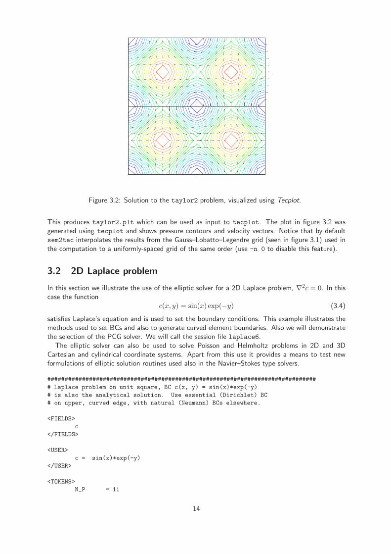
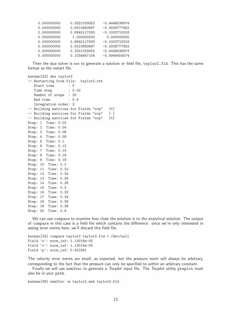
Figure 3.2: Solution to the taylor2 problem, visualized using Tecplot.

This produces taylor2.plt which can be used as input to tecplot. The plot in figure 3.2 wasgenerated using tecplot and shows pressure contours and velocity vectors. Notice that by defaultsem2tec interpolates the results from the Gauss–Lobatto–Legendre grid (seen in figure 3.1) used inthe computation to a uniformly-spaced grid of the same order (use -n 0 to disable this feature).

3.2 2D Laplace problem

In this section we illustrate the use of the elliptic solver for a 2D Laplace problem, ∇2c = 0. In thiscase the function

c(x, y) = sin(x) exp(−y) (3.4)

satisfies Laplace’s equation and is used to set the boundary conditions. This example illustrates themethods used to set BCs and also to generate curved element boundaries. Also we will demonstratethe selection of the PCG solver. We will call the session file laplace6.

The elliptic solver can also be used to solve Poisson and Helmholtz problems in 2D and 3DCartesian and cylindrical coordinate systems. Apart from this use it provides a means to test newformulations of elliptic solution routines used also in the Navier–Stokes type solvers.

##############################################################################

# Laplace problem on unit square, BC c(x, y) = sin(x)*exp(-y)

# is also the analytical solution. Use essential (Dirichlet) BC

# on upper, curved edge, with natural (Neumann) BCs elsewhere.

<FIELDS>

c

</FIELDS>

<USER>

c = sin(x)*exp(-y)

</USER>

<TOKENS>

N_P = 11

14

TOL_REL = 1e-12

STEP_MAX = 1000

</TOKENS>

<GROUPS NUMBER=4>

1 d value

2 a slope

3 b slope

4 c slope

</GROUPS>

<BCS NUMBER=4>

1 d 1

<D> c = sin(x)*exp(-y) </D>

2 a 1

<N> c = -cos(x)*exp(-y) </N>

3 b 1

<N> c = cos(x)*exp(-y) </N>

4 c 1

<N> c = sin(x)*exp(-y) </N>

</BCS>

<NODES NUMBER=9>

1 0.0 0.0 0.0

2 0.5 0.0 0.0

3 1.0 0.0 0.0

4 0.0 0.5 0.0

5 0.5 0.5 0.0

6 1.0 0.5 0.0

7 0.0 1.0 0.0

8 0.5 1.0 0.0

9 1.0 1.0 0.0

</NODES>

<ELEMENTS NUMBER=4>

1 <Q> 1 2 5 4 </Q>

2 <Q> 2 3 6 5 </Q>

3 <Q> 4 5 8 7 </Q>

4 <Q> 5 6 9 8 </Q>

</ELEMENTS>

<SURFACES NUMBER=8>

1 1 1 c 

2 2 1 c 

3 2 2 b 

4 4 2 b 

5 4 3 d 

6 3 3 d 

7 3 4 a 

8 1 4 a 

</SURFACES>

<CURVES NUMBER=1>

1 4 3 <ARC> 1.0 </ARC>

</CURVES>

15

0 0.2 0.4 0.6 0.8 1

0

0.2

0.4

0.6

0.8

1

1 2

3 4

Figure 3.3: The mesh corresponding to the laplace6 session file.

3.2.1 Curved element edges

The mesh is somewhat similar to that for the Taylor flow example, the only difference being in theuse of a curved edge for the 3rd edge of element 4, as specified in the CURVES section. Both ARC

and SPLINE type curves are currently implemented. For the ARC type, the parameter supplies theradius of the curve: a positive value implies that the curve makes the element convex on that side,while a negative value implies a concave side. Note that where elements mate along a curved side,the curve must be defined twice, once for each element, and with radii of different signs on eachside. The mesh for this problem can be seen in figure 3.3.

For the SPLINE type, the parameter supplies the name of an ASCII file which contains a list of(x, y) coordinate pairs (white-space delimited). Naturally, the list of points should be in arc-lengthorder. A single file can be used to supply the curved edges for a set of element edges. The vertices ofthe relevant elements do not have to lie exactly on the splined curve— if they do not, those verticesget shifted to the intersection of the projection of the straight line joining the original vertex positionand its neighbouring “curve-normal’ vertex, and the cubic spline joining the points in the file. Onthe other hand, it is good practise to ensure that the declared vertex locations lie close to the spline,and to check the mesh that is produced: use meshpr to do this.

3.2.2 Boundary conditions

The other new sections introduced in the session file for this example (GROUPS, BCS) are used toimpose boundary conditions on the problem. The GROUPS section associates a character group tag(e.g. d) with a string (e.g. value), but note that different groups can be associated with the samestring3. Groups a, b and c will be used to set natural (i.e. slope or Neumann), boundary conditions(∂c/∂n = value), while group a will be used to impose an essential or Dirichlet condition (c = value).

The BCS section is used to define the boundary conditions which will be applied for each group. Foreach group, after the numeric tag (ignored) appears the character for that group, then the numberof BCs that will be applied: this corresponds to the number of fields in the problem, in this case 1(c). BCs are typically of Dirichlet, Neumann, or mixed type (note that domain periodicity can be

3This allows actions to be taken over a set of BCs which share the same string.

16

employed but that this does not constitute a boundary condition). So in this case we will declarethe BC types to be D (Dirichlet) for group d and N (Neumann) for groups a, b and c. On Neumannboundaries, the value which must be supplied is the slope of the solution along the outward normalto the solution domain. Note the fact that the BCs can be set using the function parser, using thebuilt-in functions and variables, also any symbols defined in the TOKENS section, as well as the spatialvariables x, y and z. The BCs can also be functions of time, t, and for time-varying problems theboundary conditions are re-evaluated every time step.

The BC groups are associated with element edges in the SURFACES section, in a similar way tothe use of periodic boundaries for the taylor2 problem, although the edges are set to be B (BC)rather than P (periodic).

Periodic edges, Dirichlet, Neumann and mixed boundary conditions can be arbitrarily combined ina problem. Dirichlet conditions over-ride Neumann ones where they meet (say at the corner node ofan element). See further discussion on boundary conditions in § 3.5 below.


We will run the solver and compare the computed solution to the analytical solution. We will selectthe iterative (PCG) solver using the -i command-line option to elliptic, then check the resultusing compare.

karman[287] elliptic -i laplace6

-- Initializing solution with zero IC

Start time : 0

Time step : 0.01

Number of steps : 1

End time : 0.01


karman[288] compare laplace6 laplace6.fld > /dev/null

Field ’c’: norm_inf: 1.37112e-08

Next try the direct solver (default):



karman[289] elliptic laplace6

-- Initializing solution with zero IC

Start time : 0

Time step : 0.01

Number of steps : 1

End time : 0.01


-- Building matrices for Fields "c" [*]



In this case the direct solver is more accurate, but comparable accuracy with the iterative solvercould be obtained by decreasing TOL_REL in the TOKENS section (and further increasing STEP_MAX,which has a default value of 500).

17

3.3 3D Kovasznay flow

Here we will solve another viscous flow for which an analytical solution exists, the Kovasznay flow(we will call the session file kovas3). In the x–y plane, this flow is

u = 1− exp(λx) cos(2πy) (3.5)

v = λ/(2π) exp(λx) sin(2πy) (3.6)

w = 0 (3.7)

p = (1− exp(λx))/2 (3.8)

where λ = Re/2− (0.25Re2 + 4π2)1/2.Although the solution has only two velocity components, we will set up and solve the problem

in three dimensions, with a periodic length in the z direction of 1.0 and 8 z planes of data. Thelength in the z direction is set within the code by the variable BETA where β = 2π/Lz. The defaultvalue of BETA is 1, so we reset this in the TOKENS section using the function parser. The exactvelocity boundary conditions are supplied on at the left and right edges of the domain, and periodicboundaries are used on the upper and lower edges (the domain has −0.5 ≤ y ≤ 0.5). Since the flowevolves to a steady state, first order timestepping is employed (N_TIME = 1).

##############################################################################

# Kovasznay flow in the x--y plane has the exact solution

#

# u = 1 - exp(lambda*x)*cos(2*PI*y)

# v = lambda/(2*PI)*exp(lambda*x)*sin(2*PI*y)

# w = 0

# p = (1 - exp(lambda*x))/2

#

# where lambda = Re/2 - sqrt(0.25*Re*Re + 4*PI*PI).

#

# This 3D version uses symmetry planes on the upper and lower boundaries

# with flow in the x-y plane.

#

# Solution accuracy is independent of N_Z since all flow is in the x--y plane.

<USER>

u = 1.0-exp(LAMBDA*x)*cos(TWOPI*y)

v = LAMBDA/(TWOPI)*exp(LAMBDA*x)*sin(TWOPI*y)

w = 0.0

p = 0.5*(1.0-exp(LAMBDA*x))

</USER>

<FIELDS>

u v w p

</FIELDS>

<TOKENS>

N_Z = 8

N_TIME = 1

N_P = 8

N_STEP = 500

D_T = 0.008

Re = 40.0

KINVIS = 1.0/Re

LAMBDA = Re/2.0-sqrt(0.25*Re*Re+4.0*PI*PI)

Lz = 1.0

BETA = TWOPI/Lz

18

</TOKENS>

<GROUPS NUMBER=1>

1 v velocity

</GROUPS>

<BCS NUMBER=1>

1 v 4

<D> u = 1-exp(LAMBDA*x)*cos(2*PI*y) </D>

<D> v = LAMBDA/(2*PI)*exp(LAMBDA*x)*sin(2*PI*y) </D>

<D> w = 0.0 </D>

<H> p </H>

</BCS>

<NODES NUMBER=9>

1 -0.5 -0.5 0.0

2 0 -0.5 0.0

3 1 -0.5 0.0

4 -0.5 0 0.0

5 0 0 0.0

6 1 0 0.0

7 -0.5 0.5 0.0

8 0 0.5 0.0

9 1 0.5 0.0

</NODES>

<ELEMENTS NUMBER=4>

1 <Q> 1 2 5 4 </Q>

2 <Q> 2 3 6 5 </Q>

3 <Q> 4 5 8 7 </Q>

4 <Q> 5 6 9 8 </Q>

</ELEMENTS>

<SURFACES NUMBER=6>

1 1 1 3 3 

2 2 1 4 3 

3 2 2 v 

4 4 2 v 

5 3 4 v 

6 1 4 v 

</SURFACES>

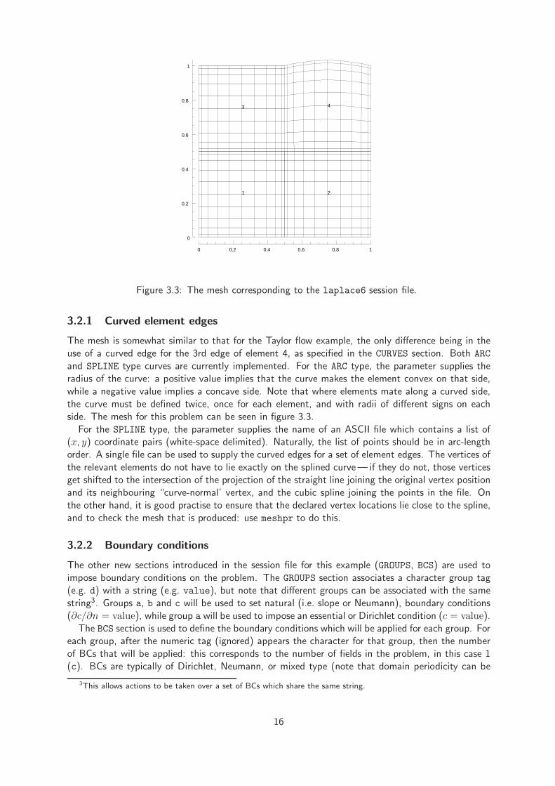
3.3.1 ‘High-order’ pressure boundary condition

Note that there is only one boundary group, and four boundary conditions must be set, correspondingto the four fields u, v, w and p. A new feature is a pressure BC of type H, which is an internally-computed Neumann boundary condition, (a High-order pressure BC) as described in Karniadakis et al.(1991). This is the kind of pressure BC that is supplied at all places except on outflow boundaries.The pressure BC is computed internally, so no value is required (if given, it will be ignored).


After running dns, we confirm there is only a single dump in the field file kovas3.fld, then runcompare in order to examine the error norms for the solution. Following that we prepare input forTecplot, projecting the interpolation to a 20× 20 grid in each element. A view of the result can beseen in figure 3.4.

karman[25] convert kovas3.fld | grep -i session

19

Figure 3.4: Solution to the kovas3 problem, visualized using Tecplot. The plot shows contours of vvelocity component and streamlines.

kovas3 Session

karman[26] compare kovas3 kovas3.fld > /dev/null

Field ’u’: norm_inf: 5.70744e-05

Field ’v’: norm_inf: 3.04095e-05

Field ’w’: norm_inf: 0

Field ’p’: norm_inf: 0.928545

karman[27] meshpr kovas3 | sem2tec -n20 kovas3.fld

3.4 Vortex breakdown—a cylindrical-coordinate problem

Here we will examine a problem which uses the cylindrical coordinate option of dns. The physicalsituation is a cylindrical cavity, H/R = 2.5 with the flow driven by a spinning lid at one end. At theReynolds number we’ll use, Re = ΩR2/ν = 2119, a vortex breakdown is known to occur. The flowin this case is invariant in the azimuthal direction, but has three velocity components (it is 2D/3C).In the cylindrical code, the order of spatial directions and velocity components is z, r, θ.

Note that for a full circle in the azimuthal direction, BETA = 1.0, (which is the default value).In fact, the value would not be used in the present solution, since all derivatives in the azimuthaldirection are implicitly zero when N_Z=1. (But see § 3.4.1 below.)

#############################################################################

# 15 element driven cavity flow.

<FIELDS>

u v w p

</FIELDS>

<TOKENS>

CYLINDRICAL = 1

N_Z = 1

BETA = 1.0

20

N_TIME = 2

N_P = 11

N_STEP = 100000

D_T = 0.01

Re = 2119

KINVIS = 1/Re

OMEGA = 1.0

TOL_REL = 1e-12

</TOKENS>

<GROUPS NUMBER=3>

1 v velocity

2 w wall

3 a axis

</GROUPS>

<BCS NUMBER=3>

1 v 4

<D> u = 0 </D>

<D> v = 0 </D>

<D> w = OMEGA*y </D>

<H> p </H>

2 w 4

<D> u = 0 </D>

<D> v = 0 </D>

<D> w = 0 </D>

<H> p </H>

3 a 4

<A> u </A>

<A> v </A>

<A> w </A>

<A> p </A>

</BCS>

<NODES NUMBER=24>

1 0 0 0

2 0.4 0 0

3 0.8 0 0

4 1.5 0 0

5 2.4 0 0

6 2.5 0 0

7 0 0.15 0

8 0.4 0.15 0

9 0.8 0.15 0

10 1.5 0.15 0

11 2.4 0.15 0

12 2.5 0.15 0

13 0 0.75 0

14 0.4 0.75 0

15 0.8 0.75 0

16 1.5 0.818 0

17 2.4 0.9 0

18 2.5 0.9 0

19 0 1 0

20 0.4 1 0

21 0.8 1 0

22 1.5 1 0

23 2.4 1 0

21

0 0.5 1 1.5 2 2.5

0

0.2

0.4

0.6

0.8

1

1 2 3 4 5

6 7 8 9 10

11 12 13 14 15

Figure 3.5: Mesh for the vortex breakdown problem. The spinning lid is at right.

24 2.5 1 0

</NODES>

<ELEMENTS NUMBER=15>

1 <Q> 1 2 8 7 </Q>

2 <Q> 2 3 9 8 </Q>

3 <Q> 3 4 10 9 </Q>

4 <Q> 4 5 11 10 </Q>

5 <Q> 5 6 12 11 </Q>

6 <Q> 7 8 14 13 </Q>

7 <Q> 8 9 15 14 </Q>

8 <Q> 9 10 16 15 </Q>

9 <Q> 10 11 17 16 </Q>

10 <Q> 11 12 18 17 </Q>

11 <Q> 13 14 20 19 </Q>

12 <Q> 14 15 21 20 </Q>

13 <Q> 15 16 22 21 </Q>

14 <Q> 16 17 23 22 </Q>

15 <Q> 17 18 24 23 </Q>

</ELEMENTS>

<SURFACES NUMBER=16>

1 1 1 a 

2 2 1 a 

3 3 1 a 

4 4 1 a 

5 5 1 a 

6 5 2 v 

7 10 2 v 

8 15 2 v 

9 15 3 w 

10 14 3 w 

11 13 3 w 

12 12 3 w 

13 11 3 w 

14 11 4 w 

15 6 4 w 

16 1 4 w 

</SURFACES>

The mesh for the problem is shown in figure 3.5, and the velocity field is shown compared to anexperimental streakline flow visualisation on the front cover of this document.

22

3.4.1 BCs for cylindrical coordinates

A new feature here is the use of BCs of type A on the axis of the flow. Internally, the code setsthe BC there either as zero essential or zero natural, depending on the physical variable and theFourier mode. Owing to the coupling scheme used in the code (Blackburn and Sherwin; 2004), theboundary conditions for the radial and azimuthal velocities v and w must be of the same type withineach group. A further restriction is that the group to which the axis belongs must have name axis.

Finally, say you wish to solve a cylindrical-coordinate problem where you know there is an n-foldazimuthal symmetry (say n = 3). In that case, it is much cheaper to solve with BETA=3, and useone-third the number of azimuthal planes that would be required for BETA=1.

3.5 Boundary condition roundup

The basic types of boundary conditions the code can deal with are Dirichlet type (value of variableis set, a.k.a. an essential boundary condition in the finite element community) and Neumann type(boundary-normal gradient of value is approximated, a.k.a. a natural type boundary condition in thefinite-element community). The code can also deal with boundary conditions of mixed type (a linearcombination of Dirichlet and Neumann). We note that periodic domain boundary surfaces () areallowed, but strictly speaking, periodicity does not constitute a boundary condition as such. Also weremark that for our code(s), boundary conditions may only be set for variables involved in ellipticsub-problems where, owing to the MWR treatment, Neumann boundary conditions are implementedas integral approximations (which converge to the given value pointwise as resolution is increased),while Dirichlet conditions are ‘lifted’ out of the problem and imposed exactly to the values which areset by the user.

Standard Dirichlet and Neumann boundary conditions may be supplied as a string that can beparsed by the solver to obtain a real value, based on predefined and user-declared TOKENS, and alsothe space/time variables x, y, z and t. These strings are re-parsed at each time step, so time-varyingboundary conditions are allowed. We have already seen examples of these BC declarations in §§ 3.2,3.3 and 3.4. Note that the strings involved should not contain white space.

We have not yet described mixed boundary conditions. These are of type ∂c/∂n+K(c−C) = 0where C and K are constants. Here, n signifies the unit outward normal direction: ∂c/∂n = n ·∇c.Mixed boundary conditions are specified in the form <M> field = mulval;refval </M> wheremulval is (a string that evaluates to) the real value K and refval is (a string that evaluates to)the real value C. At present for mixed BCs, unlike Dirichlet and Neumann boundary conditions, Cand K are fixed at the values they initially evaluate to (not time-varying).

In Navier–Stokes type problems, various of the above boundary conditions for the velocity andpressure variables are typically combined in set ways. In some cases, the user does not provide valuesor choose the combination since the boundary conditions are computed internally. Below we supplyas examples various typical boundary condition sets which would be located in the BCS section of asession file. As written, they are for two-component Navier–Stokes problems but the generalisationto three-component problems should be obvious.

See also § 3.2 of the Dog user guide for a discussion of sets of boundary condtions appropriate forsymmetry and anti-symmetry boundaries.

3.5.1 No-slip wall

<D> u = 0.0 </D>

<D> v = 0.0 </D>

<H> p </H>

The tag H for pressure (p) denotes an internally computed ’high-order’ Neumann condition, asoriginally described by Karniadakis et al. (1991). If the associated GROUP string is wall then tractions

23

will contribute to the integrated values found in session.flx file, see § 4.4.

3.5.2 Inflow or prescribed-velocity boundary

<D> u = 1.0 </D>

<D> v = 0.0 </D>

<H> p </H>

Note that either of the supplied values can be a string to be evaluated by the parser at each timestep.

3.5.3 Slip (no-penetration) boundary

<N> u = 0.0 </N>

<D> v = 0.0 </D>

<H> p </H>

Note that in this case, the boundary needs to be aligned with the x axis. At present there is no wayto set a slip boundary which is inclined or curved; it must be parallel to either the x or y axis.

3.5.4 ‘Stress-free’ outflow boundary

<N> u = 0.0 </N>

<N> v = 0.0 </N>

<D> p = 0.0 </D>

This is a restricted approximation to a true stress-free boundary where the tractions are zero. Thisboundary is also stress-free but achieves the condition by ensuring that the viscous and pressuretractions are individually zero, rather than their sum.

3.5.5 ‘Robust’ outflow boundary

<O> u </O>

<O> v </O>

<O> p </O>

This is a set of computed boundary conditions (computed Neumann for velocity and computedDirichlet for pressure). (In fact if w is included, its boundary condition is set as ∂w/∂n = 0 ratherthan being computed.) This boundary condition was originally described in Dong et al. (2014),and is based on maintaining boundedness of kinetic energy within the domain. It is excellent formaintaining stability for flows in short open domains, where the use of the ’stress-free’ conditiondescribed in § 3.5.4 can lead to catastrophe if significant inflow occurs over an outflow boundary.Type O boundaries must set the string outflow in their associated GROUP. In addition one must setthe token U0Delta (see eq. 4 of Dong et al.; 2014, this is Uoδ) which is typically of order 0.1 or less.

3.5.6 Axis boundary

<A> u </A>

<A> v </A>

<A> p </A>

This is a set of Fourier-mode dependent homogeneous Dirichlet and Neumann boundary conditions tobe used when the boundary coincides with the x axis of a cylindrical coordinate system as describedin Blackburn and Sherwin (2004). Type A boundaries must set the string axis in their associatedGROUP.

24

3.6 Fixing problems

You are liable to come up against a few generic problems when making and running your own cases.Here we will restrict discussion to Navier–Stokes problems and dns. The best diagnostic of troubleis the divergence of the solution. The code will output an estimate of the CFL-timestep everyIO_CFL timesteps (default 50), along with the average divergence of the solution (in the operator-splitting used, incompressibility is only ensured in the spatial-convergence limit). Unfortunately theCFL estimate is presently unreliable, but the divergence energy provides an excellent diagnostic oftrouble! If velocity and length scales are of order unity, the reported divergence energy should bemuch less than unity; if the divergence is large then either the solution is blowing up4, or the spatialresolution is inadequate, or both.

By far the most common problem is that the solution will have a CFL-type instability broughtabout by using too large a time-step; this instability is unavoidably associated with using explicit timeintegration for the advection terms in the Navier–Stokes equations. This problem is easily enoughfixed: try reducing D_T and increasing N_STEP to maintain the same integration interval. Obviouslyyou will typically want D_T as large as possible, so if the problem runs stably, increase the timestep asmuch as is reasonable. If the velocity and timescales are of order unity, then the maximum timestepwould typically be of order two orders of magnitude smaller (0.01). Note that CFL-stability willdecrease with increasing time-integration order (N_TIME).

If the solution persists in blowing up when the timestep is reduced, the next most common causeis that there is inflow across an outflow boundary (in which case the problem is ill-posed, however,in practice some inflow across an outflow boundary over restricted times may be present withoutcausing difficulty). To check if this is the cause, you could put some history points near the outflow(see § 4.7), but the best method of diagnosis is to run the solution up to a time when divergence startsto increase markedly, then use Tecplot or some other postprocessor to examine the solution near theoutflow. This problem has been largely circumvented in Semtex V8 using the robust outflow BC setdescribed by Dong et al. (2014), see § 3.5.5 above, though it cannot overcome all problems (e.g.an ‘outflow’ boundary with completely dominant inflow). In pathological cases of this sort, fixingthe problem will generally require the mesh to be altered: sometimes the mesh is badly structurednear the outflow (e.g. element sizes have been varied too rapidly); sometimes the problem can beovercome by extending the domain downstream; sometimes the domain needs to be reshaped (e.g. bycontracting it in the cross-flow direction) so that there will be no outflow over the inflow boundary. Ifall else fails, consider the methods of § 4.12.3 to force the velocity near the outflow to be somethingmore computationally tractable (if unphysical).

Any time you change the element polynomial order by changing N_P, or alter the structure of theboundary conditions, you should remake the numbering file session.num. It is especially importantto remember this if you have changed the structure of the boundary conditions without changingelement order, as no warning will be triggered; however, in this case you may no longer be actu-ally applying the boundary conditions you have set in the session file because the mask values insession.num (which are set to 1 along a Dirichlet-type boundary) may no longer match what isimplied by session.

3.7 Execution speed

Semtex relies heavily on the BLAS, so it can be worth seeking fast implementations. Especially,performance of matrix–matrix multiplication routine dgemm is critical. Consistently of late, KazushigeGoto’s implementation of the BLAS gives best performance and is worth seeking out, although Iunderstand his dgemm has also now been licenced to various vendors (Intel, AMD, Apple, . . . ) andis what you’ll get if you link their extended math libraries.

4One wag suggested the name Semtex was associated with this property of the solutions.

25

As Reynolds numbers increase (i.e. KINVIS decreases), the viscous Helmholtz matrices in theoperator splitting become more diagonally dominant and better conditioned. In this case, you mayfind that iterative (PCG) solution of the viscous step (obtained by setting ITERATIVE=1 or runningdns -i) is actually faster than the direct solution that is obtained by default. This is nice becauseadditionally, less memory is required. It is generally worth checking this if you plan an extended seriesof runs, and Reynolds numbers are large.

26

Chapter 4

Extra controls

This chapter describes some additional features that are implemented within the Navier–Stokes solverdns to control execution and output.

4.1 Default values of flags and internal variables

There are two simple ways to establish the default values of all the internal flags and variables usedby Semtex. The first is via the calc utility: run calc -h and check the output (this will also showyou all the functions available to the parser for calculating TOKEN variables, initial and boundaryconditions). The second is to examine the file femlib/defaults.h.

4.2 Checkpointing

By default, intermediate solutions are written out as checkpoint dumps in file session.chk everyIO_FLD steps (default value IO_FLD = 500), rotating this to session.chk.bak so there are usuallytwo checkpoint files available for restarting if execution stops prematurely (e.g. if terminated by aqueuing system or by a floating point error). Once the final time (N_STEP) is reached, the outcome(the termimal solution field) is written to session.fld.

Sometimes however, one wants a sequence of field dumps to be written to session.fld. Onecan toggle this behaviour on the command line using dns -chk, or alternatively set the TOKEN

CHKPOINT=0 (the default being CHKPOINT=1). Note that turning off checkpointing can result in thegeneration of extremely large session.fld files.

4.3 Iterative solution

Two matrix solution methods are implemented for Helmholtz problems associated with the viscoussubstep of the time splitting. By default, direct Schur-complement solutions are used. The associatedglobal matrices can consume quite large amounts of memory, typically much more than is requiredfor storage of the associated field variable. Iterative (PCG) solution can also be selected, and this hasthe advantage that since it is matrix-free, no global matrices are required, however, solution may beslower than for the direct solver (depending on the condition number of the global matrix problem).

The token that controls the selection of matrix solution method is ITERATIVE. For dns, PCGsolution can be selected for the viscous substep of the solution (ITERATIVE = 1). This can alsobe selected via a command-line option (dns -i), but note that this overridden by tokens set in thesession file (the default value is ITERATIVE = 0).

Iterative solution can be useful for the viscous substep, particularly when the Reynolds number ishigh, since this decreases the condition number of the associated global matrices. In fact, iterativesolutions for the viscous substep can execute faster than direct solutions at high Reynolds number,

27

although this is platform dependent. You should always consider trying ITERATIVE = 1 as an optionfor simulations where the Reynolds number is more than a few hundred.

4.4 Wall fluxes

A file called session.flx is used to store the integral over the wall group boundaries of viscous andpressure stresses (i.e. lift and drag forces). Output is done every IO_HIS steps. For each direction(x, y, z), the outputs are in turn the pressure, viscous, and total force per unit length. In 2D thez-components are always zero, while in 3D the z-component pressure force is always zero, owing tothe fact that the geometry is invariant in that direction. For cylindrical geometries, the output valuesare forces per radian (in the x and y directions) and torque per radian (in the z direction) ratherthan forces per unit length.

4.5 Wall tractions

If the token IO_WSS is set to a non-zero value then the normal and the single (2D) or two (3D)components of tangential boundary traction are computed on the wall group, and output everyIO_WSS steps in the file session.wss. This is a binary file with structure similar to a field dump.The utility wallmesh is used to extract the corresponding mesh points along the walls (and can beused with sem2tec to produce Tecplot input files). Note also that there is a stand-alone utility calledtraction which is a post-processor that takes a standard .fld file and produces a wall traction file.

4.6 Modal energies

For three-dimensional simulations (N_Z > 2), a file of modal energies, session.mdl, is produced.This provides valuable diagnostic information for turbulent flow simulations. For each active Fouriermode k in the simulation, the value output every IO_HIS steps is

Ek =1

2A

∫

Ω

u∗

k · uk dΩ,

where A is the area of the 2D domain Ω. (In cylindrical coordinate problems, the integrand ismultiplied by radius.) Each line of the file contains the time t, mode number k and Ek.

We note that the energies are output only for non-negative Fourier modes. To get the correctestimates for the one-sided spectrum (and to satisfy Parseval’s relation), the energies for non-zeromodes should be doubled.

4.7 History points

History points are used to record solution variables at fixed spatial locations as the simulation pro-ceeds. The locations need not correspond to grid points, as data are interpolated onto the givenspatial locations using the elemental basis functions. Locations of history points are declared in thesession file as follows:

<HISTORY NUMBER=1>

# tag x y z

1 0 0 0

</HISTORY>

A file called session.his is produced as output. Each line of the file contains the step number,the time, the history point tag number, followed by values for each of the solution variables. Thestep interval at which history point information is dumped to file is controlled by the IO_HIS token;the default value is IO_HIS = 10.

28

4.8 Averaging

Set AVERAGE = 1 in the tokens section to get averages of field variables left in files session.ave andsession.avg (which are analogous to session.chk and session.fld, but session.ave.bak isnot produced). Averages are updated every IO_HIS steps, and dumped every IO_FLD steps. Restartsare made by reading session.avg if it exists.

Setting AVERAGE = 2 will accumulate averages for Reynolds stresses as well, with reserved namesABCDEF, corresponding to products

uu uv uw A B D

vv vw = C E

ww F

The hierarchy is named this way to allow accumulation of products in 2D as well as 3D (for 2D youget only ABC). In order to actually compute the Reynolds stresses from the accumulated productsyou need to run the rstress utility, which subtracts the products of the means from the means ofthe products:

rstress session.avg > reynolds-stress.fld

An alternative function of rstress is to subtract one field file from another:

rstress good.fld test.fld | convert | diff

Setting AVERAGE = 3 will accumulate sums of additional products for computation of terms inthe energy transport equation. You will then need to use the eneq utility to actually compute theterms. Presently this part of the code is only written for Cartesian coordinates.

4.9 Phase averaging

Phase averaging is useful for turbulent flows with a dominant (and known) underlying temporalperiod. We can collect statistics (with AVERAGE=1, 2 or 3)—much as for the case without phaseaveraging enabled—conditional on phase in the cycle of the underlying period, see Reynolds andHussain (1972). Turning on phase averaging does not preclude or stop collection of standard statis-tics. The enabling token is N_PHASE, which must be a positive integer; in addition one needs tokenSTEPS_P (steps per period) which must be chosen such that STEPS_P modulo N_PHASE is zero, andalso N_STEP modulo N_PHASE must be zero and IO_FLD=STEPS_P/N_PHASE. Statistics are writtento files session.0.phs . . . session.X.phs where X=N_PHASE-1. The Reynolds stresses computedfrom these files will represent fluctuations around the conditional average flow at each phase point(the so-called ‘triple decomposition’).

The slight difficulty is that if the period is not very well-defined or we have a poor estimate ofit, our sampling phase will slowly drift unless we take corrective action. However if the underlyingperiod is very well defined (e.g. the flow is periodically forced) the method has great potential.

4.10 Particle tracking

The code allows for tracking of massless particles, but this only works correctly for non-concurrentexecution at present. Tracking is quite an expensive operation, since Newton–Raphson iteration isused to relocate particles within each element at every timestep.

The application looks for a file called session.par. Each line of this file is of form

# tag time ctime x y z

1 0.0 0.0 1.0 10.0 0.5.

29

The time value is the integration time, while ctime records the time at which integration wasinitialised.

Output is of the same form, and is called session.trk. The use of separate files, rather than bydeclaration in the session file, is intended so that session.trk files can be moved to session.par

files for restarting. Particles that aren’t in the domain at startup, or leave the domain duringexecution, are deleted.

Setting SPAWN = 1, re-initiates extra particles at the original positions every timestep. Withspawning, particle tracking can quickly grow to become the most time-consuming part of execution.

4.11 Spectral vanishing viscosity

Spectral vanishing viscosity (SVV) amounts to implementing larger viscosity at higher wavenumberseither in Fourier space or in spectral element polynomial space. The idea is that as resolution isincreased via p-refinement, the effect ‘vanishes’ (Tadmor; 1989; Maday et al.; 1993). One may regardSVV either as a type of implicit large-eddy simulation methodology (Pasquetti; 2006) or as a means ofstabilizing spectral element solutions especially at high Reynolds numbers (Xu and Pasquetti; 2004;Kirby and Sherwin; 2006). Neither of these ideas has firm theoretical underpinning at this stage,yet the method does appear quite effective in reducing resolution requirements for turbulent flowsimulations (Koal et al.; 2012; Chin et al.; 2015). Our implementation and nomenclature follows the‘standard method’ described in Koal et al. (2012). One can turn on SVV separately and with differentparameters for (x, y) spectral elements and in the Fourier (z) direction. These are all declared in theTOKENS section.

SVV MN Corresponds to cut-in mode Mzr in spectral elements. Must be less than N P.SVV MZ Corresponds to cut-in mode Mϕ in Fourier direction. Must be less than N Z/2.SVV EPSN Corresponds to εzr. Should be a value larger than KINVIS, e.g. 5*KINVIS.SVV EPSZ Corresponds to εϕ. A value larger than KINVIS.

The default polynomial transform in to place spectral element expansions into a discrete hierar-chical space is the discrete Legendre transform (see e.g. Blackburn and Schmidt; 2003). This canbe changed in src/svv.cpp.

4.12 General body forcing

This extension was developed by Thomas Albrecht.

If found, the FORCE section of the session file allows you to declare various types of body forcing,i.e. add a source term to the RHS of the Navier–Stokes equation. The currently implemented typesinclude (any combination allowed):

f = fconst constant force+ a1(x) steady, but spatially varying force+ a2(x)α(t) modulated force− m1(x) (u − u0) sponge region− m2(x) (u/|u|) |u(x, t)|

2 ‘drag’ force+ ǫG white noise− χ(u− u) selective frequency damping− 2 Ω× u− (dΩ/dt)× x−Ω×Ω× x Coriolis force.

For example, a force constant in time and space f = fconst is declared by:

30

<FORCE>

CONST_X = 4

CONST_Y = 0

CONST_Z = 0

</FORCE>

This type of forcing must not be time or space dependent. It is suitable for periodic channel flow,where you have a uniform and steady force driving the flow, see channel-FX for an example session.

Except for the constant force, all forcing terms are applied in physical space.Unless otherwise noted, any skipped keyword defaults to 0. Any line starting with a hash # is

ignored.

4.12.1 Steady force

A spatially varying, steady force f = a(x), computed (or read from a file) during pre-processing andapplied every time step. See box-steady for the complete example session. It suits applicationsrequiring localised, steady forcing.

<FORCE>

STEADY_X = cos(x)

STEADY_Y = -sin(z)

STEADY_Z = -cos(y)

# STEADY_FILE = box-steady.force.fld

</FORCE>

You may also point STEADY_FILE to a field file, in which case the force is taken from the uvw

fields of that file and STEADY_[XZY] is ignored.

4.12.2 Modulated force

A spatially varying force, which is modulated in time, f = a(x)α(t). The steady part a(x) iscomputed (or read from a file) during pre-processing, while α(t) is evaluated each time step.

<FORCE>

# -- spatially varying part

MOD_A_X = cos(x)

MOD_A_Y = -sin(z)

MOD_A_Z = -cos(y)

# MOD_A_FILE = box-mod.force.fld

# -- time varying part

MOD_ALPHA_X = step(t, 10)

MOD_ALPHA_Y = step(t, 10)

MOD_ALPHA_Z = step(t, 10)

</FORCE>

4.12.3 Sponge region

This implements a so-called ‘sponge region’ defined by the shape functionm(x) in which a (physicallymeaningless) penalty term f = m(x) (u − u0) forces the flow towards a given solution u0. It isespecially useful for inflow–outflow simulations of vortex shedding or turbulence: if the velocityfluctuations hit the outflow boundary condition, they cause unphysical reflections back into thedomain which distort the upstream flow. A sponge region placed just upstream the outflow boundaryhelps to reduce the velocity fluctuations to (near) zero and thereby prevents those reflections. The

31

following section would apply the penalty term for 20 ≤ x ≤ 24, and within that region forces thevelocity to approach (1, 0, 0). That given solution may be a function of space, but must be steady.

<FORCE>

SPONGE_M = 5. * step(x,20)*heav(24-x)

SPONGE_U = 1

SPONGE_V = 0

SPONGE_W = 0

</FORCE>

4.12.4 ’Drag’ force

An approximate drag force f = −m(x) (u/|u|) |u(x, t)|2. Be aware that we use the previous timestep’s velocity un here.

<FORCE>

DRAG_M = heav((x-2)^2 + y^2, 0.25)

</FORCE>

4.12.5 White noise force

Similar to the noiz tool, this continuously adds random perturbation f = (ǫx, ǫy, ǫz)T G in specified

direction, where G is a normal distributed random variable. Setting WHITE_MODE ≥ 0 perturbs thegiven mode only, i.e. WHITE_MODE = 2 will perturb mode 2 only. Omitting this keyword or settingWHITE_MODE < 0 will apply white noise to all modes.

The following example applies white noise in x−direction to mode 0:

<FORCE>

WHITE_MODE = 0

WHITE_EPS_X = 0.1

WHITE_EPS_Y = 0

WHITE_EPS_Z = 0

</FORCE>

Adding white noise in all three directions degrades performance by about 10%.

4.12.6 Selective frequency damping (SFD)

This is a means of obtaining an approximate steady state solution to the Navier–Stokes equationsusing an unsteady solver, originally described by Akervik et al. (2006). SFD applies a penalty term ofthe form −χ(u− u) to the right-hand side of the momentum equations, where u is an estimate ofthe time-mean solution that is updated as integration proceeds (and held in internal storage). SFDcan also be considered as applying an IIR low-pass digital filter to the discrete approximation of theNavier–Stokes equations.

The two parameters are SFD_CHI (i.e. penalization multiplier χ) and SFD_DELTA, which is the timeconstant ∆ used in updating a forwards-Euler approximation of the steady flow u (see reference).Both values are problem-specific and should be tuned to get acceptable results. Note that it isnot always possible to obtain a steady outcome with SFD, and that it is generally preferable to usestandard skew-symmetric form of the nonlinear terms for dns, rather than the now-default alternatingskew symmetric form: this can be achieved by setting token ADVECTION = 0 or by using command-line flag -S with dns.

<FORCE>

SFD_CHI = 0.2

32

SFD_DELTA = 0.75

</FORCE>

4.12.7 Rotating frame of reference: Coriolis and centrifugal force

If the flow is to be computed in a rotating frame of reference, additional acceleration terms appear,namely f = −2Ω×u− (dΩ/dt)×x−Ω× (Ω×x) (Batchelor; 1967). The vector of rotation Ω isalways given in Cartesian co-ordinates, even if CYLINDRICAL = 1. Its magnitude and/or orientationcan change with time. However, the axis of rotation it is always assumed to go through the origin.Depending on whether Ω is steady or not, usage slightly differs.

For unsteady Ω, set the flag CORIOLIS_UNSTEADY = 1 and give Ω and dΩ/dt. All terms arere-evaluated each time step.

<TOKENS>

f = 1.

omega = TWOPI * f

</TOKENS>

<FORCE>

CORIOLIS_UNSTEADY = 1

CORIOLIS_OMEGA_X = 0

CORIOLIS_OMEGA_Y = 0

CORIOLIS_OMEGA_Z = omega * sin(t)

CORIOLIS_DOMEGA_X_DT = 0

CORIOLIS_DOMEGA_Y_DT = 0

CORIOLIS_DOMEGA_Z_DT = omega * cos(t)

</FORCE>

For constant Ω 6= f(t), the term −(dΩ/dt)× x vanishes, and the centrifugal force −Ω× (Ω× x)can be computed during pre-processing. Set CORIOLIS_UNSTEADY = 0 and make sure to includethe centrifugal force manually using a steady force as it is no longer computed automatically1. Atemporal derivative dΩ/dt, if given, is ignored.

<FORCE>

CORIOLIS_UNSTEADY = 0

CORIOLIS_OMEGA_X = 0

CORIOLIS_OMEGA_Y = 0

CORIOLIS_OMEGA_Z = omega

# -- centrifugal term for Omega = (0, 0, omega)^T

# for a cylindrical problem

STEADY_X = x*omega^2

STEADY_Y = omega^2*y*(cos(z)^2)

STEADY_Z = -omega^2*y*cos(z)*sin(z)

</FORCE>

See Albrecht et al. (2015) for an example of DNS carried out in a rotating frame of reference.

1If you’re lazy, or for cross-checking, you could set CORIOLIS UNSTEADY = 1 and omit CORIOLIS DOMEGA [XYZ] DT

to have the centrifugal term computed automatically. Note, however, that this degrades performance as it is done eachtime step.

33

Chapter 5

Specialised executables

The special compilations below can be combined.

5.1 Concurrent execution

The code supports concurrent execution for 3D simulations, with MPI used as the message-passingkernel. Compile using make MPI=1 to produce dns_mp. (You will also need to compile in theappropriate message-passing routines in compiling femlib, for which change to the femlib directory,then do make clean; make MPI=1; make install MPI=1.) Nonlinear terms are not dealiasedwhen running in parallel, but are dealiased in the Fourier direction when running on one process, orrunning the serial code. To get a serial code that does not perform dealiasing on Fourier terms (e.g.for cross-checking), compile the serial code using make ALIAS=1 to produce dns_alias (in whichcase make sure you delete nonlinear.o first).

5.2 Vector architectures

The code has a fair amount of low-level optimisation built in for vector computer architectures, butit’s not compiled in by default. To get vector-optimised routines, add -D_VECTOR_ARCH to the sectionof src/Makefile appropriate to your machine. Also you may want to try altering the parameterLVR in src/temfftd.F if your job makes heavy use of FFTs.

34

Chapter 6

Code design and the Semtex API

This chapter is in development.

While the top level of the code is written in C++, the bulk of computational work is carried outusing 3rd-party libraries: BLAS and LAPACK (vendor- or distribution-supplied) for 2D operations,Temperton’s 2-3-5 prime factor FFT (incorporated into femlib) for 3D operations, and (open)MPIfor parallel operations. Depending on what your application hits the hardest, one or other of thesethings may be the speed-determining component. Optimizing compilers are liable to make a only asmall difference—most speed-up is now to be achieved by algorithm development.

Some fundamental design decisions:

1. Most real-type data arrays are flat, 1D, zero-indexed, i.e. the same as employed in FORTRAN,and this makes them easy to use with FORTRAN routines.

2. The layout of these flat arrays are typically taken as row-major, which is standard C/C++.However, FORTRAN uses column-major ordering. For this reason, any BLAS or LAPACKoperation may at first sight seem to be the transpose of what is intended.

3. Most low-level C++ methods in the code do not incorporate internal data storage but can beregarded as operator routines, and get handed addresses to appropriate parts of storage fromwithin the flat data arrays on which to work.

Coding conventions:

1. Class private or protected member data names start with an underscore, e.g. ntot.

6.1 Useful things to know about

1. Directory layout. The following directories are present in the distribution: include whichhas copies of header files; src which holds C++ source code for the classes shared by Sem-tex applications; veclib which holds routines for many standard loops over vectors, with amnemonic naming convention (the code here is almost exclusively written in C); femlib hasone-dimensional spectral polynomial routines (knot and quadrature point computations, dif-ferentiation matrix construction) and FFTs, all written in either C or FORTRAN77; utilityroutines for pre and post-processing; test which has code validity regression tests, with the‘right answers’ stored in regress; mesh holds a selection of session files. The two main appli-cation code directories are elliptic and dns which have been described in earlier chapters.The sm directory contains useful SuperMongo macros.

2. Hierarchy of main data storage: domain, fields, auxfields, elements. The key entity for mostapplications programming is the AuxField class, which contains scalar field variables and a

35

list of Element pointers. The Field class inherits from the AuxField class, adding a list ofboundary condition applicators and the ability to solve elliptic problems. The Domain classholds an array of Field pointers and most of its internal storage is publicly accessible.

3. Nodal elements: the shape functions used in the code correspond to the classical ‘nodal’,rather than the ‘modal’ scheme. This means that the shape functions are tensor products of1D Lagrange interpolants that have value unity at one mesh node and zero at the others.

4. Timestepping algorithm and the code loop The scheme is the ‘stiffly stable’ scheme, based onbackward differencing in time, and uses time-splitting, see Karniadakis et al. (1991). What isstored where, and when — see figure 6.1.

5. Boundary conditions, use of inheritance Distinction between the way BCs are dealt with.Periodicity not a boundary condition.

6. Support libraries and static member functions. BLAS-conformant increments.

7. The parser and what things can be parsed.

8. What is done in the driver routine and the basic idea of code layout.

9. Implications of Fourier transform in one direction For 3D computations, note that for all ofthe timestepping loop, other than during computation of the nonlinear terms, field variablesare help in the Fourier-transformed state.

10. Tensor-product derivative operations.

11. Direct versus iterative solves.

12. Static condensation.

13. Message passing and data exchange.

6.2 Altering the code

If you want to alter the supplied source code, the first thing you need to know is that make willseek to resolve source file names in the current directory first, before looking elsewhere (e.g. thesrc directory, the include directory). This means that the best strategy is to copy (if not alreadypresent) only the relevant files which you need to change into your current development directory,typically from the src directory, and alter these. This way your new version does not interfere withthe supplied code base, and it is also readily apparent exactly which files you have had to change.

For example, say you want to add some new functionality to the AuxField class, within the dnsapplication. Make a clean copy of the source files (Makefile, *.C, *.h) in dns to another directoryat the same level. In that directory, place copies of auxfield.C and (if required) auxfield.h from../src and then work on these.

Testing. Typically when adding code features you want to be sure that you haven’t broken existingfunctionality. The easy way to check is to use the testregress script in the test directory. It willtell you if the code passes or fails standard regression tests which exercise most code features.

36

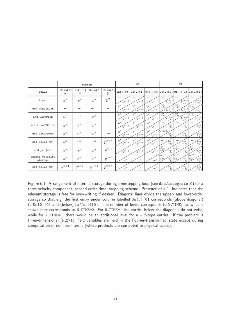
STAGE

Start

end nonLinear

end waveProp

start setPForce

end setPForce

end Solve (P)

end project

update velocity

storage

end solve (U)

Domain Us Uf

D->u[0] D->u[1] D->u[2] D->u[3]Us[.][0] Us[.][1] Us[.][2] Uf[.][2]Uf[.][1]Uf[.][0]

Figure 6.1: Arrangement of internal storage during timestepping loop (see dns/integrate.C) for athree-velocity-component, second-order-time, stepping scheme. Presence of a ’-’ indicates that therelevant storage is free for over-writing if desired. Diagonal lines divide the upper- and lower-orderstorage so that e.g. the first entry under column labelled Us[.][0] corresponds (above diagonal)to Us[0][0] and (below) to Us[1][0]. The number of levels corresponds to N TIME; i.e. what isshown here corresponds to N TIME=2. For N TIME=1 the entries below the diagonals do not exist,while for N TIME=3, there would be an additional level for n − 2-type entries. If the problem isthree-dimensional (N Z>1), field variables are held in the Fourier-transformed state except duringcomputation of nonlinear terms (where products are computed in physical space).

37

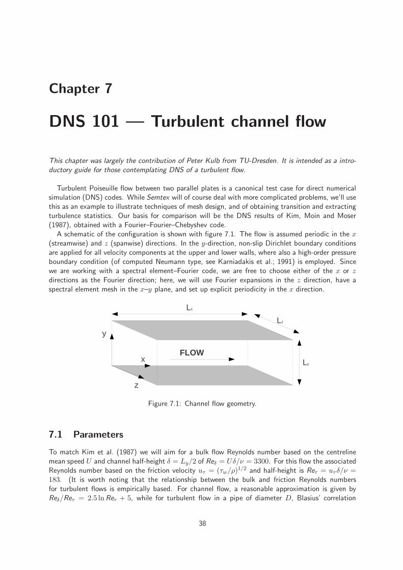
Chapter 7

DNS 101 — Turbulent channel flow

This chapter was largely the contribution of Peter Kulb from TU-Dresden. It is intended as a intro-ductory guide for those contemplating DNS of a turbulent flow.

Turbulent Poiseuille flow between two parallel plates is a canonical test case for direct numericalsimulation (DNS) codes. While Semtex will of course deal with more complicated problems, we’ll usethis as an example to illustrate techniques of mesh design, and of obtaining transition and extractingturbulence statistics. Our basis for comparison will be the DNS results of Kim, Moin and Moser(1987), obtained with a Fourier–Fourier–Chebyshev code.

A schematic of the configuration is shown with figure 7.1. The flow is assumed periodic in the x(streamwise) and z (spanwise) directions. In the y-direction, non-slip Dirichlet boundary conditionsare applied for all velocity components at the upper and lower walls, where also a high-order pressureboundary condition (of computed Neumann type, see Karniadakis et al.; 1991) is employed. Sincewe are working with a spectral element–Fourier code, we are free to choose either of the x or zdirections as the Fourier direction; here, we will use Fourier expansions in the z direction, have aspectral element mesh in the x–y plane, and set up explicit periodicity in the x direction.

Figure 7.1: Channel flow geometry.

7.1 Parameters

To match Kim et al. (1987) we will aim for a bulk flow Reynolds number based on the centrelinemean speed U and channel half-height δ = Ly/2 of Reδ = Uδ/ν = 3300. For this flow the associatedReynolds number based on the friction velocity uτ = (τw/ρ)

1/2 and half-height is Reτ = uτδ/ν =183. (It is worth noting that the relationship between the bulk and friction Reynolds numbersfor turbulent flows is empirically based. For channel flow, a reasonable approximation is given byReδ/Reτ = 2.5 lnReτ + 5, while for turbulent flow in a pipe of diameter D, Blasius’ correlation

38

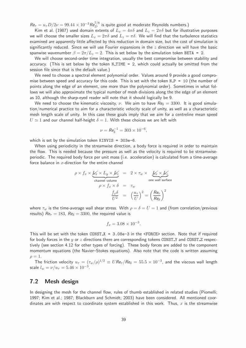
Reτ = uτD/2ν = 99.44 × 10−3Re7/8D is quite good at moderate Reynolds numbers.)

Kim et al. (1987) used domain extents of Lx = 4πδ and Lz = 2πδ but for illustrative purposeswe will choose the smaller sizes Lx = 2πδ and Lz = πδ. We will find that the turbulence statisticsexamined are apparently little affected by this reduction in domain size, but the cost of simulation issignificantly reduced. Since we will use Fourier expansions in the z direction we will have the basicspanwise wavenumber β = 2π/Lz = 2. This is set below by the simulation token BETA = 2.

We will choose second-order time integration, usually the best compromise between stability andaccuracy. (This is set below by the token N TIME = 2, which could actually be omitted from thesession file since that is the default value.)

We need to choose a spectral element polynomial order. Values around 9 provide a good compro-mise between speed and accuracy for this code. This is set with the token N P = 10 (the number ofpoints along the edge of an element, one more than the polynomial order). Sometimes in what fol-lows we will also approximate the typical number of mesh divisions along the the edge of an elementas 10, although the sharp-eyed reader will note that it should logically be 9.

We need to choose the kinematic viscosity, ν. We aim to have Reδ = 3300. It is good simula-tion/numerical practice to aim for a characteristic velocity scale of unity, as well as a characteristicmesh length scale of unity. In this case these goals imply that we aim for a centreline mean speedU ≃ 1 and our channel half-height δ = 1. With these choices we are left with

ν = Re−1

δ = 303 × 10−6,

which is set by the simulation token KINVIS = 303e-6.When using periodicity in the streamwise direction, a body force is required in order to maintain

the flow. This is needed because the pressure as well as the velocity is required to be streamwise-periodic. The required body force per unit mass (i.e. acceleration) is calculated from a time-averageforce balance in x-direction for the entire channel

ρ× fx ×Lx × Ly ×Lz︸︷︷︸

channel volume

= 2× τw × Lx ×Lz︸︷︷︸

one wall surface

ρ× fx × δ = τw

fxδ

U2=

(uτU

)2

=

(ReτReδ

)2

where τw is the time-average wall shear stress. With ρ = δ = U = 1 and (from correlation/previousresults) Reτ = 183, Reδ = 3300, the required value is

fx = 3.08 × 10−3.

This will be set with the token CONST X = 3.08e-3 in the <FORCE> section. Note that if requiredfor body forces in the y or z directions there are corresponding tokens CONST Y and CONST Z respec-tively (see section 4.12 for other types of forcing). These body forces are added to the componentmomentum equations (the Navier–Stokes equations). Also note that the code is written assumingρ = 1.

The friction velocity uτ = (τw/ρ)1/2 ≡ UReτ/Reδ = 55.5 × 10−3, and the viscous wall length

scale lw = ν/uτ = 5.46 × 10−3.

7.2 Mesh design

In designing the mesh for the channel flow, rules of thumb established in related studies (Piomelli;1997; Kim et al.; 1987; Blackburn and Schmidt; 2003) have been considered. All mentioned coor-dinates are with respect to coordinate system established in this work. Thus, x is the streamwise

39

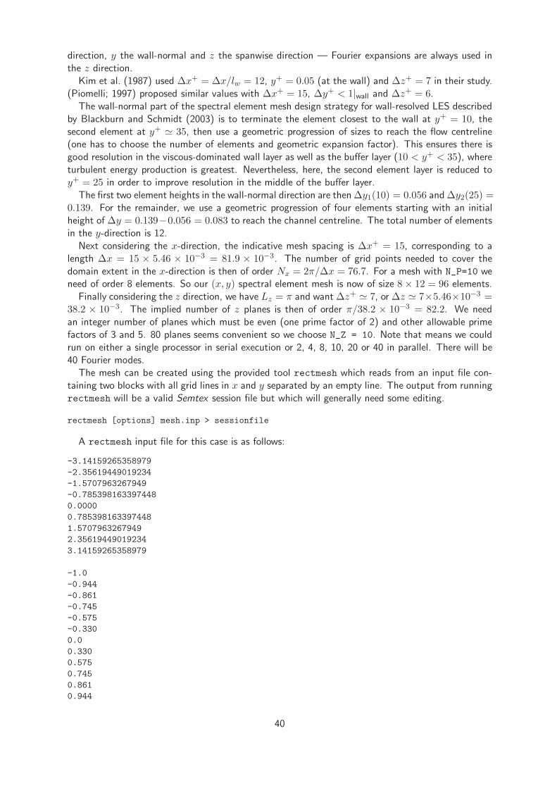
direction, y the wall-normal and z the spanwise direction — Fourier expansions are always used inthe z direction.

Kim et al. (1987) used ∆x+ = ∆x/lw = 12, y+ = 0.05 (at the wall) and ∆z+ = 7 in their study.(Piomelli; 1997) proposed similar values with ∆x+ = 15, ∆y+ < 1|wall and ∆z+ = 6.

The wall-normal part of the spectral element mesh design strategy for wall-resolved LES describedby Blackburn and Schmidt (2003) is to terminate the element closest to the wall at y+ = 10, thesecond element at y+ ≃ 35, then use a geometric progression of sizes to reach the flow centreline(one has to choose the number of elements and geometric expansion factor). This ensures there isgood resolution in the viscous-dominated wall layer as well as the buffer layer (10 < y+ < 35), whereturbulent energy production is greatest. Nevertheless, here, the second element layer is reduced toy+ = 25 in order to improve resolution in the middle of the buffer layer.

The first two element heights in the wall-normal direction are then∆y1(10) = 0.056 and∆y2(25) =0.139. For the remainder, we use a geometric progression of four elements starting with an initialheight of ∆y = 0.139−0.056 = 0.083 to reach the channel centreline. The total number of elementsin the y-direction is 12.

Next considering the x-direction, the indicative mesh spacing is ∆x+ = 15, corresponding to alength ∆x = 15 × 5.46 × 10−3 = 81.9 × 10−3. The number of grid points needed to cover thedomain extent in the x-direction is then of order Nx = 2π/∆x = 76.7. For a mesh with N_P=10 weneed of order 8 elements. So our (x, y) spectral element mesh is now of size 8× 12 = 96 elements.

Finally considering the z direction, we have Lz = π and want ∆z+ ≃ 7, or ∆z ≃ 7×5.46×10−3 =38.2 × 10−3. The implied number of z planes is then of order π/38.2 × 10−3 = 82.2. We needan integer number of planes which must be even (one prime factor of 2) and other allowable primefactors of 3 and 5. 80 planes seems convenient so we choose N_Z = 10. Note that means we couldrun on either a single processor in serial execution or 2, 4, 8, 10, 20 or 40 in parallel. There will be40 Fourier modes.

The mesh can be created using the provided tool rectmesh which reads from an input file con-taining two blocks with all grid lines in x and y separated by an empty line. The output from runningrectmesh will be a valid Semtex session file but which will generally need some editing.

rectmesh [options] mesh.inp > sessionfile

A rectmesh input file for this case is as follows:

-3.14159265358979

-2.35619449019234

-1.5707963267949

-0.785398163397448

0.0000

0.785398163397448

1.5707963267949

2.35619449019234

3.14159265358979

-1.0

-0.944

-0.861

-0.745

-0.575

-0.330

0.0

0.330

0.575

0.745

0.861

0.944

40

1.0

Once this file is built, all the above mentioned parameters can be changed to their desired value.Also, the boundary conditions have to be named and set into place. We use wall boundary conditionson the upper and lower edges of the domain, and edit the <SURFACES> section to obtain periodicityin the streamwise direction. Here the example input file for this particular case:

################################################################

# 96 element channel flow, for Re_bulk = 3300, Re_tau = 183

<FIELDS>

u v w p

</FIELDS>

<USER>

u = 1.0-y*y

v = 0.0

w = 0.0

p = 0.0

</USER>

<TOKENS>

N_TIME = 2

N_P = 10

N_Z = 80

BETA = 2.0

N_STEP = 60000

D_T = 0.002

KINVIS = 303e-6

IO_CFL = 100

IO_HIS = 100

AVERAGE = 2

</TOKENS>

<FORCE>

CONST_X = 3.08e-3

</FORCE>

<GROUPS NUMBER=1>

1 w wall

</GROUPS>

<BCS NUMBER=1>

1 w 4

<D> u = 0.0 </D>

<D> v = 0.0 </D>

<D> w = 0.0 </D>

<H> p </H>

</BCS>

<NODES NUMBER=117>

1 -3.14159 -1 0

...

117 3.14159 1 0

</NODES>

<ELEMENTS NUMBER=96>

1 <Q> 1 2 11 10 </Q>

41

...

96 <Q> 107 108 117 116 </Q>

</ELEMENTS>

<SURFACES NUMBER=28>

1 1 1 w 

2 2 1 w 

3 3 1 w 

4 4 1 w 

5 5 1 w 

6 6 1 w 

7 7 1 w 

8 8 1 w 

9 89 3 w 

10 90 3 w 

11 91 3 w 

12 92 3 w 

13 93 3 w 

14 94 3 w 

15 95 3 w 

16 96 3 w 

17 8 2 1 4 

18 16 2 9 4 

19 24 2 17 4 

20 32 2 25 4 

21 40 2 33 4 

22 48 2 41 4 

23 56 2 49 4 

24 64 2 57 4 

25 72 2 65 4 

26 80 2 73 4 

27 88 2 81 4 

28 96 2 89 4 

</SURFACES>

<HISTORY NUMBER=1>

1 0.0 0.0 0.0

</HISTORY>

7.3 Initiating and monitoring transition

The critical bulk Reynolds number for linear instability of channel flow is Rec = 5772 but turbulencecan typically be maintained down to lower values (and here we are aiming at Reδ = 3300) if transitionis obtained. Our strategy here will be to start from a laminar flow profile and add some white noiseto obtain transition. This is done using the following single line to generate an initial condition:

compare chan | noiz -p 0.1 chan.fld > chan.rst

Here, the command-line value 0.1 represents the standard deviation of the normal/Gaussian dis-tribution from which the noise is derived using a pseudorandom number generator and is thereforequite large compared to an average velocity of U = 1. It is necessary, since our Reynolds numberis here below the critical value, to assure a sufficient amount of disturbance to initiate transitionto a turbulent state. If the Reynolds number were above the critical value, any perturbation levelabove machine noise level should eventually produce transition — it just depends on how long youare prepared to wait. We note that channel flow is a case for which it is relatively easy to obtaintransition to turbulence without carefully manipulating the noise level, or restricting the time step.

42

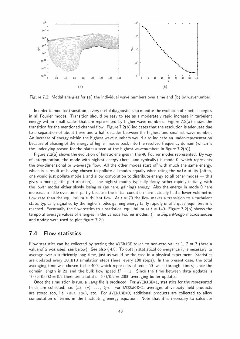
10-14

10-12

10-10

10-8

10-6

10-4

10-2

100

0 20 40 60 80 100 120 140 160

E(k

)

t

(a)

10-7

10-6

10-5

10-4

10-3

0 5 10 15 20 25 30 35 40

E(k

)

k

(b)

Figure 7.2: Modal energies for (a) the individual wave numbers over time and (b) by wavenumber.

In order to monitor transition, a very useful diagnostic is to monitor the evolution of kinetic energiesin all Fourier modes. Transition should be easy to see as a moderately rapid increase in turbulentenergy within small scales that are represented by higher wave numbers. Figure 7.2(a) shows thetransition for the mentioned channel flow. Figure 7.2(b) indicates that the resolution is adequate dueto a separation of about three and a half decades between the highest and smallest wave number.An increase of energy within the highest wave numbers would also indicate an under-representationbecause of aliasing of the energy of higher modes back into the resolved frequency domain (which isthe underlying reason for the plateau seen at the highest wavenumbers in figure 7.2(b)).

Figure 7.2(a) shows the evolution of kinetic energies in the 40 Fourier modes represented. By wayof interpretation, the mode with highest energy (here, and typically) is mode 0, which representsthe two-dimensional or z-average flow. All the other modes start off with much the same energy,which is a result of having chosen to pollute all modes equally when using the noiz utility (often,one would just pollute mode 1 and allow convolution to distribute energy to all other modes — thisgives a more gentle perturbation). The highest modes typically decay rather rapidly initially, withthe lower modes either slowly losing or (as here, gaining) energy. Also the energy in mode 0 hereincreases a little over time, partly because the initial condition here actually had a lower volumetricflow rate than the equilibrium turbulent flow. At t ≈ 70 the flow makes a transition to a turbulentstate, typically signalled by the higher modes gaining energy fairly rapidly until a quasi-equilibrium isreached. Eventually the flow settles to a statistical equilibrium at t ≈ 140. Figure 7.2(b) shows thetemporal average values of energies in the various Fourier modes. (The SuperMongo macros modenand modav were used to plot figure 7.2.)

7.4 Flow statistics

Flow statistics can be collected by setting the AVERAGE token to non-zero values 1, 2 or 3 (here avalue of 2 was used, see below). See also § 4.8. To obtain statistical convergence it is necessary toaverage over a sufficiently long time, just as would be the case in a physical experiment. Statisticsare updated every IO_HIS simulation steps (here, every 100 steps). In the present case, the totalaveraging time was chosen to be 400, which represents of order 60 ‘wash-through’ times, since thedomain length is 2π and the bulk flow speed U = 1. Since the time between data updates is100 × 0.002 = 0.2 there are a total of 400/0.2 = 2000 averaging buffer updates.

Once the simulation is run, a .avg file is produced. For AVERAGE=1, statistics for the representedfields are collected, i.e. 〈u〉, 〈v〉, . . . , 〈p〉. For AVERAGE=2, averages of velocity field productsare stored too, i.e. 〈uu〉, 〈uv〉, etc. For AVERAGE=3, additional products are collected to allowcomputation of terms in the fluctuating energy equation. Note that it is necessary to calculate

43

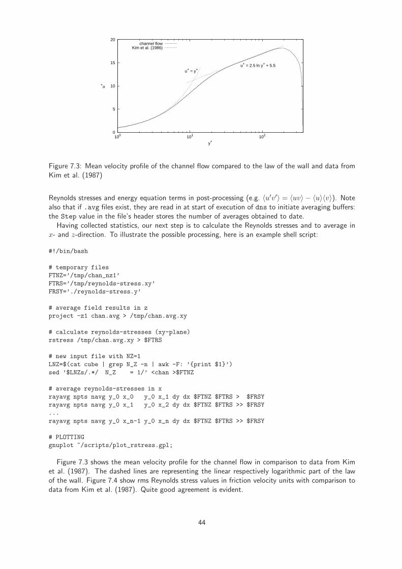
0

5

10

15

20

100 101 102

u+

y+

u+ = y+u+ = 2.5 ln y+ + 5.5

channel flowKim et al. (1986)

Figure 7.3: Mean velocity profile of the channel flow compared to the law of the wall and data fromKim et al. (1987)

Reynolds stresses and energy equation terms in post-processing (e.g. 〈u′v′〉 = 〈uv〉 − 〈u〉〈v〉). Notealso that if .avg files exist, they are read in at start of execution of dns to initiate averaging buffers:the Step value in the file’s header stores the number of averages obtained to date.

Having collected statistics, our next step is to calculate the Reynolds stresses and to average inx- and z-direction. To illustrate the possible processing, here is an example shell script:

#!/bin/bash

# temporary files

FTNZ=’/tmp/chan_nz1’

FTRS=’/tmp/reynolds-stress.xy’

FRSY=’./reynolds-stress.y’

# average field results in z

project -z1 chan.avg > /tmp/chan.avg.xy

# calculate reynolds-stresses (xy-plane)

rstress /tmp/chan.avg.xy > $FTRS

# new input file with NZ=1

LNZ=$(cat cube | grep N_Z -n | awk -F: ’print $1’)

sed ’$LNZs/.*/ N_Z = 1/’ <chan >$FTNZ

# average reynolds-stresses in x

rayavg npts navg y_0 x_0 y_0 x_1 dy dx $FTNZ $FTRS > $FRSY

rayavg npts navg y_0 x_1 y_0 x_2 dy dx $FTNZ $FTRS >> $FRSY

...

rayavg npts navg y_0 x_n-1 y_0 x_n dy dx $FTNZ $FTRS >> $FRSY

# PLOTTING

gnuplot ~/scripts/plot_rstress.gpl;

Figure 7.3 shows the mean velocity profile for the channel flow in comparison to data from Kimet al. (1987). The dashed lines are representing the linear respectively logarithmic part of the lawof the wall. Figure 7.4 show rms Reynolds stress values in friction velocity units with comparison todata from Kim et al. (1987). Quite good agreement is evident.

44

0.0

0.5

1.0

1.5

2.0

2.5

3.0

-1.0 -0.5 0.0 0.5 1.0

u rm

s , v

rms

, wrm

s

y/δ

urms

vrms

wrms


0.0

0.5

1.0

1.5

2.0

2.5

3.0

0 10 20 30 40 50 60 70 80

u rm

s , v

rms

, wrm

s

y+

urms

vrms

wrms


Figure 7.4: Root-mean-squares velocity fluctuations in global coordinates normalized by the wallshear velocity uτ . Comparison to data from Kim et al. (1987).

45

Bibliography

Akervik, E., Brandt, L., Henningson, D. S., Hœpfner, J., Marxen, O. and Schlatter, P. (2006).Steady solutions to the Navier–Stokes equations by selective frequency damping, Phys. Fluids18: 068102–1–4.

Albrecht, T., Blackburn, H. M., Lopez, J. M., Manasseh, R. and Meunier, P. (2015). Triadicresonances in precessing rapidly rotating cylinder flows, J. Fluid Mech. 778: R–1–11.

Amon, C. H. and Patera, A. T. (1989). Numerical calculation of stable three-dimensional tertiarystates in grooved-channel flow, Phys. FluidsA 1(2): 2005–2009.

Batchelor, G. K. (1967). An Introduction to Fluid Dynamics, Cambridge University Press.Blackburn, H. M. (2001). Dispersion and diffusion in coated tubes of arbitrary cross-section, Com-

puters and Chem. Eng. 25(2/3): 313–322.Blackburn, H. M. (2002a). Mass and momemtum transport from a sphere in steady and oscillatory

flows, Phys. Fluids 14(11): 3997–4011.Blackburn, H. M. (2002b). Three-dimensional instability and state selection in an oscillatory axisym-

metric swirling flow, Phys. Fluids 14(11): 3983–3996.Blackburn, H. M. (2003). Computational bluff body fluid dynamics and aeroelasticity, in N. G.

Barton and J. Periaux (eds), Coupling of Fluids, Structures and Waves Problems in Aeronautics,Notes in Numerical Fluid Mechanics, Springer, pp. 10–23.

Blackburn, H. M., Barkley, D. and Sherwin, S. J. (2008). Convective instability and transient growthin flow over a backward-facing step, J. Fluid Mech. 603: 271–304.

Blackburn, H. M., Govardhan, R. N. and Williamson, C. H. K. (2000). A complementary numericaland physical investigation of vortex-induced vibration, J. Fluids & Struct. 15(3/4): 481–488.

Blackburn, H. M. and Henderson, R. D. (1996). Lock-in behaviour in simulated vortex-inducedvibration, Exptl Thermal & Fluid Sci. 12(2): 184–189.

Blackburn, H. M. and Henderson, R. D. (1999). A study of two-dimensional flow past an oscillatingcylinder, J. Fluid Mech. 385: 255–286.

Blackburn, H. M. and Lopez, J. M. (2003a). On three-dimensional quasi-periodic Floquet instabilitiesof two-dimensional bluff body wakes, Phys. Fluids 15(8): L57–60.

Blackburn, H. M. and Lopez, J. M. (2003b). The onset of three-dimensional standing and modulatedtravelling waves in a periodically driven cavity flow, J. Fluid Mech. 497: 289–317.

Blackburn, H. M., Marques, F. and Lopez, J. M. (2005). Symmetry breaking of two-dimensionaltime-periodic wakes, J. Fluid Mech. 522: 395–411.

Blackburn, H. M. and Schmidt, S. (2003). Spectral element filtering techniques for large eddysimulation with dynamic estimation, J. Comput. Phys. 186(2): 610–629.

Blackburn, H. M. and Sherwin, S. J. (2004). Formulation of a Galerkin spectral element–Fouriermethod for three-dimensional incompressible flows in cylindrical geometries, J. Comput. Phys.197(2): 759–778.

Blackburn, H. M. and Sherwin, S. J. (2007). Instability modes and transition of pulsatile stenoticflow: Pulse-period dependence, J. Fluid Mech. 573: 57–88.

Canuto, C., Hussaini, M. Y., Quarteroni, A. and Zang, T. A. (1988). Spectral Methods in FluidDynamics, Springer, Berlin.

46

Canuto, C., Hussaini, M. Y., Quarteroni, A. and Zang, T. A. (2006). Spectral Methods: Fundamen-tals in Single Domains, Springer.

Canuto, C., Hussaini, M. Y., Quarteroni, A. and Zang, T. A. (2007). Spectral Methods: Evolutionto Complex Geometries and Applications in Fluid Dynamics, Springer.

Chin, C., Ng, H. C. N., Blackburn, H. M., Monty, J. and Ooi, A. S. H. (2015). Turbulent pipe flowat Reτ = 1000: a comparison of wall-resolved large-eddy simulation, direct numerical simulationand hot-wire experiment, Computers and Fluids . to appear.

Deville, M. O., Fischer, P. F. and Mund, E. H. (2002). High-Order Methods for Incompressible FluidFlow, Cambridge University Press.

Dong, S., Karniadakis, G. E. and Chryssostomidis, C. (2014). A robust and accurate outflowboundary condition for incompressible flow simulations on severely-truncated unbounded domains,J. Comput. Phys. 261: 83–105.

Elston, J. R., Blackburn, H. M. and Sheridan, J. (2006). The primary and secondary instabilities offlow generated by an oscillating circular cylinder, J. Fluid Mech. 550: 359–389.

Funaro, D. (1997). Spectral Elements for Transport-Dominated Equations, Vol. 1 of Lecture Notesin Computational Science and Engineering, Springer, Berlin.

Gottlieb, D. and Orszag, S. A. (1977). Numerical Analysis of Spectral Methods: Theory and Appli-cations, SIAM.

Guermond, J. L., Minev, P. and Shen, J. (2006). An overview of projection methods for incompressibleflows, Comp. Meth. Appl. Mech. & Engng 195: 6011–6045.

Guermond, J. L. and Shen, J. (2003). Velocity-correction projection methods for incompressibleflows, SIAM J. Numer. Anal. 41(1): 112–134.

Henderson, R. D. (1999). Adaptive spectral element methods for turbulence and transition, inT. J. Barth and H. Deconinck (eds), High-Order Methods for Computational Physics, Springer,chapter 3, pp. 225–324.

Henderson, R. D. and Karniadakis, G. E. (1995). Unstructured spectral element methods for simu-lation of turbulent flows, J. Comput. Phys. 122: 191–217.

Karniadakis, G. E. (1989). Spectral element simulations of laminar and turbulent flows in complexgeometries, Appl. Num. Math. 6: 85–105.

Karniadakis, G. E. (1990). Spectral element–Fourier methods for incompressible turbulent flows,Comp. Meth. Appl. Mech. & Engng 80: 367–380.

Karniadakis, G. E. and Henderson, R. D. (1998). Spectral element methods for incompressible flows,in R. W. Johnson (ed.), Handbook of Fluid Dynamics, CRC Press, Boca Raton, chapter 29,pp. 29–1–29–41.

Karniadakis, G. E., Israeli, M. and Orszag, S. A. (1991). High-order splitting methods for theincompressible Navier–Stokes equations, J. Comput. Phys. 97(2): 414–443.

Karniadakis, G. E. and Sherwin, S. J. (2005). Spectral/hp Element Methods for Computational FluidDynamics, 2nd edn, Oxford University Press.

Kim, J., Moin, P. and Moser, R. (1987). Turbulence statistics in fully developed channel flow at lowReynolds number, J. Fluid Mech. 177: 133–166.

Kirby, R. M. and Sherwin, S. J. (2006). Stabilisation of spectral/hp element method through spectralvanishing viscosity: application to fluid mechanics modelling, Comp. Meth. Appl. Mech. & Engng195: 3128–3144.

Koal, K., Stiller, J. and Blackburn, H. M. (2012). Adapting the spectral vanishing viscosity methodfor large-eddy simulations in cylindrical configurations, J. Comput. Phys. 231: 3389–3405.

Korczak, K. Z. and Patera, A. T. (1986). An isoparametric spectral element method for solution ofthe Navier–Stokes equations in complex geometry, J. Comput. Phys. 62: 361–382.

Maday, Y., Kaber, S. M. O. and Tadmor, E. (1993). Legendre pseudospectral viscosity method fornonlinear conservation laws, SIAM J. Num. Anal. 30: 321–342.

Maday, Y. and Patera, A. T. (1989). Spectral Element Methods for the Incompressible Navier–StokesEquations, State-of-the-Art Surveys on Computational Mechanics, ASME, chapter 3, pp. 71–143.

47

Pasquetti, R. (2006). Spectral vanishing viscosity methods for large-eddy simulation of turbulentflows, J. Sci. Comp. 27(1–3): 365–375.

Patera, A. T. (1984). A spectral element method for fluid dynamics: Laminar flow in a channelexpansion, J. Comput. Phys. 54: 468–488.

Piomelli, U. (1997). Large-eddy simulations: Where we stand, in C. Liu and Z. Liu (eds), Advancesin DNS/LES, AFOSR, Louisiana, pp. 93–104.

Reynolds, W. C. and Hussain, A. K. M. F. (1972). The mechanics of an organized wave in tur-bulent shear flow. Part 3. Theoretical models and comparisons with experiments, J. Fluid Mech.41(2): 263–288.

Rudman, M. and Blackburn, H. M. (2006). Direct numerical simulation of turbulent non-Newtonianflow using a spectral element method, Appl. Math. Mod. 30(11): 1229–1248.

Sherwin, S. J. and Blackburn, H. M. (2005). Three-dimensional instabilities and transition of steadyand pulsatile flows in an axisymmetric stenotic tube, J. Fluid Mech. 533: 297–327.

Tadmor, E. (1989). Convergence of spectral methods for nonlinear conservation laws, SIAM J. Num.Anal. 26(1): 30–44.

Xu, C. and Pasquetti, R. (2004). Stabilized spectral element computations of high Reynolds numberincompressible flows, J. Comput. Phys. 196: 680–704.

Zang, T. A. (1991). On the rotation and skew-symmetric forms for incompressible flow simulations,Appl. Num. Math. 7: 27–40.

48

Documents

Using Semtex - User Web Pages - Monash University