Embed Size (px)
Citation preview

Using Securities Market Information for BankSupervisory Monitoring∗
John Krainer and Jose A. LopezEconomic Research Department, Federal Reserve Bank of San Francisco
U.S. bank supervisors conduct comprehensive inspectionsof bank holding companies and assign them a supervisory rat-ing, known as a BOPEC rating prior to 2005, meant to summa-rize their overall condition. We develop an empirical model ofthese BOPEC ratings that combines supervisory and securitiesmarket information. Securities market variables, such as stockreturns and bond yield spreads, improve the model’s in-samplefit. Debt market variables provide more information on super-visory ratings for banks closer to default, while equity marketvariables provide useful information on ratings for banks fur-ther from default. The out-of-sample accuracy of the modelwith securities market variables is little different from thatof a model based on supervisory variables alone. However,the model with securities market information identifies addi-tional ratings downgrades, which are of particular importanceto bank supervisors who are concerned with systemic risk andcontagion.
JEL Codes: G14, G21.
∗The views expressed here are those of the authors and not necessarily thoseof the Federal Reserve Bank of San Francisco or the Federal Reserve System.We thank Rob Bliss for generously sharing his bank holding company debt data-base with us. We thank Hyun Song Shin (the editor), an anonymous referee,Fred Furlong, Reint Gropp, and seminar participants at the Bank of England,the Basel Committee’s Research Task Force on Banking Supervision, and theChicago Conference on Bank Competition and Structure for helpful sugges-tions. We thank Judy Peng Feria, Ryan Stever, and Chishen Wei for researchassistance. E-mails: Krainer: [email protected]; Lopez: [email protected].
125
126 International Journal of Central Banking March 2008
1. Introduction
The most comprehensive tool for banking supervision in the UnitedStates is the on-site inspection, where a team of supervisors visits aninstitution and analyzes its operations in detail. For bank holdingcompanies (BHCs), Federal Reserve examiners assign the institu-tion a rating, known as a BOPEC rating up through 2004, at theconclusion of an inspection. The rating summarizes the examiners’opinion of the BHC’s overall financial condition. On-site inspectionsare conducted on roughly an annual basis. Between BHC on-siteinspections, examiners engage in off-site monitoring, which largelyconsists of analyzing quarterly reports from the institutions in ques-tion. However, BHCs that have outstanding public securities arealso being monitored by their equity shareholders and debtholders.Since their assessments of BHCs have been found to be timely andaccurate in previous studies, the aim of this paper is to investi-gate the effectiveness of BHC securities market data, both from theequity and debt markets, in off-site monitoring models of BOPECratings.1
Securities market prices should, in an ideal world, tell supervisorsall they need to know about a BHC’s condition and its likelihood offailure. In practice, however, there are various frictions that makeour questions worthy of empirical research. First, perceptions of pos-sible government support for a struggling BHC, and the depositorysafety net in general, might reduce investor incentives to monitor.This would potentially decrease the sensitivity of security prices tochanges in BHC conditions. Second, since banks specialize in solvingproblems of asymmetric information, the loans they hold as assetsmay be difficult for outside investors to value. This problem, likethe first, might make security prices less sensitive to changes in assetvalue. Finally, supervisors have access to information that BHCs arenot normally required to disclose to investors, raising questions ofwhether securities prices can tell supervisors anything they do notalready know.
1Note that in this paper we focus on supervisory ratings and not defaults,another key supervisory concern. There exists an extensive literature on bankdefault dating back to Meyer and Pifer (1970), Sinkey (1975), and Pettway andSinkey (1980).

Vol. 4 No. 1 Using Securities Market Information 127
In this paper, we seek to accomplish three main objectives. First,we investigate the potential contributions of both equity and debtmarket information to the supervisory monitoring of BHCs using anoff-site monitoring model for BOPEC ratings. We measure the con-tributions of these variables relative to a model based on supervisorydata alone.2
The second objective of our study is to investigate the cases wheninformation from the equity or debt markets is relatively more useful.We find an asymmetric contribution from these variables for predict-ing BOPEC rating changes that depends on how close a BHC’s assetsare to its default point. That is, in a model of BOPEC changes, themagnitude of the coefficients on equity variables is larger for BHCsfurther from default, while the coefficients on the debt variables arelarger for BHCs close to default.
Finally, our third objective is to conduct a set of realistic fore-casting exercises aimed at assessing the value of securities marketdata to bank supervisors over the last banking cycle. We find littleevidence of improved forecast performance after incorporating secu-rities market information into the off-site monitoring model. Theperformance of BOPEC forecasts based on supervisory data aloneis not statistically different from that of BOPEC forecasts gener-ated by the model augmented with securities market data. However,we find that while the forecasts are not different in a statisticalsense, they are different in an economic sense. The forecasts basedon the model incorporating securities market information identifyadditional BOPEC rating changes, especially downgrades, of pub-licly traded BHCs that were not identified by a benchmark modelbased just on supervisory data. Given a supervisory objective func-tion that values early warnings of potential downgrades, this iden-tification of additional correct BOPEC changes could outweigh thecost of additional false signals.
An extensive academic literature regarding the complementar-ity of supervisory and financial market monitoring of BHCs andtheir subsidiary banks already exists; see Flannery (1998) for asurvey. The majority of the recent studies in the literature have
2Throughout the paper, we use the term “supervisory data” to mean datagenerated by supervisors as part of the BHC quarterly reporting process or aspart of the supervisory process.
128 International Journal of Central Banking March 2008
focused on the various uses of bond market data for monitoring. Forexample, Flannery and Sorescu (1996) and Covitz, Hancock, andKwast (2004a, 2004b) study how the sensitivity of bank bond priceschanged with the passage of the FDIC Improvement Act, an eventthat arguably lessened the probability that bondholders would bebailed out in case of a bank failure. DeYoung et al. (2001) find thatbank subordinated debt prices do not immediately reflect informa-tion generated by supervisors, but that this information does enterprices over several quarters. Evanoff and Wall (2002) find that sub-ordinated debt spreads do as well or better than standard capitalratios at explaining supervisory ratings.
Relatively less attention has been paid to the value of equitymarket data for supervisory monitoring; for surveys of this work,see Krainer and Lopez (2003, 2004). Even less research has focusedon combining equity and debt market data, although there are twonotable exceptions. Berger, Davies, and Flannery (2000) examinethe timeliness and accuracy of supervisory and market assessmentsof the condition of large BHCs. They find that, after accountingfor market assessments, balance sheet variables do not contributesubstantially to the modeling of future indicators of BHC perfor-mance, such as changes in nonperforming loans, book equity cap-ital, and return on assets. Their findings suggest that supervisors,bond market participants, and equity market participants producecomplementary but different information on BHC performance.
Gropp, Vesala, and Vulpes (2004, 2006) examine the ability ofequity market variables and subordinated bond spreads for Euro-pean banks to signal changes in their agency ratings.3 Using orderedlogit models at several horizons and a proportional hazard model,they find that both equity-based measures of distance to defaultand subordinated debt spreads are useful for detecting changes inbank ratings. Interestingly, they find that the distance-to-defaultmeasure performs less well closer to default and that subordinateddebt spreads seem to have signal value only close to default. Theauthors argue that their empirical results provide support for theuse of securities market information in supervisors’ early-warningmodels.
3See also Gropp and Richards (2001).
Vol. 4 No. 1 Using Securities Market Information 129
Our paper differs from the prior studies in several importantways. As in Berger, Davies, and Flannery (2000), we use data on U.S.bank holding company condition, but our analysis focuses squarelyon supervisory ratings as the key measure of BHC condition. Thus,our analysis addresses the benefits of using market information topredict variables that supervisors care most about. Additionally,we extend their in-sample analysis to an out-of-sample forecastingframework that mimics the way supervisors might actually use secu-rities market data as a supervisory tool. Finally, though we find alimited use of securities market information for forecasting BHC con-dition, we establish the conditions at the BHC under which equityand debt market signals can be useful. Our results provide clearempirical reasoning for the Berger, Davies, and Flannery (2000)finding that supervisory and debt-related assessments of BHCs arerelated. Thus, our results are a refinement of their finding that super-visory and equity market indicators are not interrelated; i.e., we findthat abnormal BHC stock returns do provide useful information withrespect to changes in supervisory assessments when BHCs are farfrom their default points.
The paper proceeds as follows. In section 2, we provide a briefoverview of the supervisory process for BHCs in the United States.In section 3, we estimate our proposed BOPEC off-site monitor-ing model (BOM) using both supervisory and securities marketvariables. We also examine the differential impact of the securitiesmarket variables based on the BHCs’ relative distances from theirdefault points. In section 4, we examine the model’s out-of-sampleperformance using a statistical and a supervisory objective function.Section 5 concludes.
2. The U.S. Supervisory Process
The Federal Reserve is the supervisor of bank holding companiesin the United States. Full-scope, on-site inspections of BHCs are akey element of this supervisory process. These inspections are gener-ally conducted on an annual basis, particularly for the case of largeand complex BHCs.4 Limited and targeted inspections that may or
4A complex BHC is defined as one with material credit-extending nonbanksubsidiaries or debt outstanding to the general public. See DeFerrari and Palmer

130 International Journal of Central Banking March 2008
may not be conducted on-site are also carried out. In this paper, wefocus on full-scope, on-site inspections since they provide the mostcomprehensive supervisory assessments of BHCs.
At the conclusion of an inspection, supervisors assign the BHC anumerical rating, which prior to 2005 was called a composite BOPECrating, that summarizes their opinion of the BHC’s overall healthand financial condition.5 The BOPEC acronym stands for the fivekey areas of supervisory concern: the condition of the BHC’s Banksubsidiaries, Other nonbank subsidiaries, Parent company, Earnings,and Capital adequacy. A BOPEC rating of 1 is the best rating, witha rating of 5 being the worst rating short of closure. A rating of 1or 2 indicates that the BHC is not considered to be of supervisoryconcern. Note that BOPEC ratings, as well as all other inspectionmaterials, are confidential and are not made publicly available.
Between on-site inspections, when private supervisory informa-tion cannot be gathered as readily, supervisors monitor BHCs usingquarterly regulatory reports filed by BHCs and their subsidiarybanks. In addition, the supervisory CAMELS ratings assigned tobanks within the holding company are used for monitoring the par-ent BHCs. As with BOPEC ratings, CAMELS ratings are confiden-tial ratings that are assigned after a bank examination. The acronymrefers to the six key areas of concern: the bank’s Capital adequacy,Asset quality, Management, Earnings, Liquidity, and Sensitivity torisk. The composite CAMELS rating also ranges in integer valuefrom 1 to 5 in decreasing order (i.e., banks that perform best areassigned a rating of 1). Since the condition of a BHC is closelyrelated to the condition of its subsidiary banks, the off-site BHC sur-veillance program includes monitoring recently assigned CAMELSratings.
As with on-site BHC inspections, on-site bank examinationsoccur at approximately a yearly frequency, which is long enoughfor the gathered supervisory information to decay and become less
(2001) for an overview of the supervisory process for large, complex bankingorganizations.
5Note that in January 2005, the BOPEC rating system was replaced by theRFI/C(D) rating system; see Board of Governors of the Federal Reserve Sys-tem (2004). For an international survey of supervisory bank rating systems, seeSahajwala and van den Bergh (2000).
Vol. 4 No. 1 Using Securities Market Information 131
representative of the bank’s condition.6 To address this issue, theFederal Reserve instituted an off-site monitoring system for banks,known as the System for Estimating Examiner Ratings (SEER),in 1993. The SEER system actually consists of two separate mod-els that forecast bank failures over a two-year horizon as well asbank CAMELS ratings for the next quarter. The model that weare most interested in here is the latter, which is an ordered logitmodel with five categories corresponding to the five possible valuesof the CAMELS rating. The model is estimated every quarter inorder to reflect the most recent relationship between the selectedfinancial ratios and the two most recent quarters of CAMELSratings. Significant changes in a bank’s CAMELS rating as fore-casted by the SEER model could be sufficient to warrant closermonitoring of the bank. The off-site BHC surveillance programalso explicitly monitors the SEER model’s forecasted CAMELSratings.
2.1 The BOPEC Ratings Sample
The core database for our analysis is the set of supervisory BOPECratings assigned after on-site, full-scope inspections between the firstquarter of 1990 and the second quarter of 1998. The sample endpointis dictated by the availability of the bond data set.7 Our sampleof BOPEC ratings is further refined to include only those inspec-tions of top-tier BHCs with identifiable lead banks, four quarters ofprior supervisory data, and at least one prior BOPEC rating. Wefocus on top-tier BHCs since they are typically the legal entitieswithin the banking group that issues publicly traded equity. Thelead-bank designation is often provided by banks in their regula-tory filings. When such self-reporting is not available, we assign thelead-bank designation to the largest bank within the group. We needthe BHCs in our sample to have identifiable lead banks in order todirectly link their BOPEC ratings to their lead bank’s CAMELS
6See Cole and Gunther (1998) as well as Hirtle and Lopez (1999) for furtherdiscussion of this issue.
7We are grateful to Rob Bliss for sharing his BHC bond database with us. Acomplete description of the database is presented in Bliss and Flannery (2001).The last quarter of bond data is the first quarter of 1998, which aligns with thesecond quarter of 1998 in our modeling framework.
132 International Journal of Central Banking March 2008
ratings.8 Finally, we require each BHC to have at least four quar-ters of supervisory data and a lagged BOPEC rating in order toavoid issues regarding de novo BHCs and new BHCs arising frommergers. In addition, four quarters of supervisory data are requiredto calculate certain explanatory variables for the model describedbelow.
Table 1 summarizes our sample of 3,010 BOPEC ratings assignedto 1,034 unique entities. Almost 65 percent of the BHCs in the sam-ple are relatively small, with less than $1 billion in total assets.Slightly more inspections occurred in the first half of the sam-ple than in the second half, reflecting consolidation in the U.S.banking sector. For publicly traded BHCs, there are 1,291 BOPECassignments corresponding to 363 unique entities. Note that pub-lic BHCs are generally larger than privately held BHCs, with agreater percentage having total assets ranging between $1 billionand $100 billion. Of the 41 BOPECs assigned to the largest BHCs,39 are of public BHCs. With respect to BHCs with public debtoutstanding, this subsample contains 309 BOPEC ratings corre-sponding to 63 unique BHCs. Again, these BHCs are typicallylarger than those in the full sample, with almost all BHCs hav-ing between $1 billion and $100 billion in assets. Finally, there are283 BOPEC ratings corresponding to 58 unique BHCs that haveboth publicly traded equity and debt outstanding during the sampleperiod.
Tables 2A and 2B present the distribution of BOPEC ratingsassigned in each year for all BHCs, as well as for BHCs with bothpublicly traded equity and publicly traded bonds. The distributionsin the two tables share many common features. The majority of theratings fall in the upper two categories, indicating that a BHC’sfinancial condition and risk profile are of little supervisory concern.For the full sample, while the distribution of ratings fluctuates overtime, the percentage of ratings in the top two categories never fallsbelow 63 percent. The maximum value is 96 percent in 1998. Incontrast, for larger BHCs with both public equity and debt, thepercentage of ratings in the upper two categories ranges from 47
8Note that this restriction does not imply that we limited the sample to single-bank BHCs. We simply focus on the CAMELS rating for a BHC’s lead bank,whether self-identified or identified by asset size.

Vol. 4 No. 1 Using Securities Market Information 133
Table 1. Asset Size Characteristics of the BHCsin the BOPEC Sample
1990–98 1990–94 1995–98
Total # Ratings 3,010 1,735 1,275Asset Size:
Assets > $100b 41 13 28$1b < Assets < $100b 1,019 594 425Assets < $1b 1,950 1,128 822
Total # Ratings, Public BHCs 1,291 741 550Asset Size:
Assets > $100b 39 13 26$1b < Assets < $100b 807 487 320Assets < $1b 445 241 204
Total # Ratings, BHCs 309 174 135with Public Debt
Asset Size:Assets > $100b 37 11 26$1b < Assets < $100b 270 163 107Assets < $1b 2 0 2
Total # Ratings, Public BHCs 283 163 120with Public DebtAsset Size:
Assets > $100b 36 11 25$1b < Assets < $100b 247 152 95Assets < $1b 0 0 0
Note: The data sample spans the period from the first quarter of 1990 to the sec-ond quarter of 1998. The definition of a bank holding company (BHC) used in thistable is the definition used in constructing our data set; i.e., a top-tier BHC withan identifiable lead bank, four quarters of available regulatory reporting data, and alagged BOPEC rating. Public debt here refers to publicly traded bonds as listed inthe Warga/Lehmann data set and used by Bliss and Flannery (2001).
percent in 1991 to 100 percent from 1996 onward. Note that thereare relatively few inspections culminating in a BOPEC rating of 4 orworse, with the exception of the early 1990s. This likely reflects thefact that both supervisors and bankers actively try to prevent this

134 International Journal of Central Banking March 2008
Table 2A. All BOPEC Ratings in the Sample
BOPEC Rating % of Total
1 2 3 4–5
1990 16% 52% 21% 10%1991 16% 47% 25% 12%1992 15% 52% 20% 14%1993 24% 55% 14% 7%1994 34% 53% 8% 5%1995 36% 52% 8% 5%1996 47% 47% 5% 1%1997 47% 48% 4% 0%1998 47% 49% 3% 0%
Total 31% 51% 12% 6%
Note: The data sample spans the period from the first quarter of 1990 to the secondquarter of 1998.
Table 2B. All BOPEC Ratings for BHCs with PublicEquity and Bonds in the Sample
BOPEC Rating % of Total
1 2 3 4–5
1990 21% 55% 17% 7%1991 12% 35% 31% 23%1992 18% 41% 26% 15%1993 24% 68% 3% 6%1994 45% 50% 5% 0%1995 44% 56% 0% 0%1996 60% 40% 0% 0%1997 58% 42% 0% 0%1998 68% 32% 0% 0%
Total 38% 48% 9% 5%
Note: The data sample spans the period from the first quarter of 1990 to the secondquarter of 1998.

Vol. 4 No. 1 Using Securities Market Information 135
outcome, as well as the general good health of the banking sector inthe mid and late 1990s.
3. Multivariate Analysis Using the Ordered Logit Model
Our proposed BOPEC off-site monitoring (BOM) model is anordered logit model and is similar in structure to the SEER modelfor CAMELS ratings; see Krainer and Lopez (2003, 2004) for furtherdetails.9 The model assumes that the supervisory rating assigned toBHC i in quarter t is a continuous variable, denoted BP∗
it , for whichonly discrete values, denoted BPit , are observed. Recall that lowervalues of BP∗
it and BPit correspond to better supervisory ratings.We model the continuous variable as
BP∗it = βxit−2 + εit . (1)
In this specification, xit−2 is a (k×1) vector of supervisory variablesunique to BHC i observed two quarters prior to the BOPEC assign-ment. We chose to lag the supervisory variables by two quartersbecause, in real time, these are often the most recent data availableat the time of inspection.10
For firms with publicly traded securities, we augment equation(1) with securities market data, which is denoted as zit−1; i.e.,
BP∗it = βxit−2 + πzit−1 + εit . (2)
The vector zit−1 contains securities market variables—equity marketvariables, debt market variables, or both depending on the model—corresponding to BHC i at time t − 1, one quarter prior to theBOPEC assignment. The supervisory variables and the securitiesmarket variables enter into the model with different lags becausesecurities market data are available on a more timely basis thanare the supervisory variables that we use. The error term εit hasa standard logistic distribution. Note that we estimate four BOM
9Recall that Gropp, Vesala, and Vulpes (2004, 2006) used logit and propor-tional hazard models, which are better suited for examination of the timing anddeterminants of banks’ Fitch/IBCA ratings changes.
10See Gunther and Moore (2003) for further discussion.

136 International Journal of Central Banking March 2008
models corresponding to the four alternative zit−1 vectors usingBOPEC samples based on the availability of securities market vari-ables. For example, we estimate the core model without securi-ties market variables (i.e., zit−1 = 0) on all BOPEC ratings, butwe estimate the BOM model using both sets of market variablesonly on the BOPEC sample for which both sets of variables areavailable.
3.1 Supervisory Variables
The choice of which supervisory variables to include in xit−2 is chal-lenging. No simple behavioral models exist of how supervisors assignBOPEC ratings. As mentioned, there are more than 800 variables atthe supervisors’ disposal for this purpose. For this study, we selectednine explanatory variables that were judged to be reasonable prox-ies for the five components of the BOPEC rating. In addition, weincluded lagged BOPEC ratings in the specification to control forratings persistence. As in Krainer and Lopez (2003, 2004), we chosea parsimonious specification in the hopes of generating reasonableout-of-sample forecasts.
Our supervisory variables are summarized in table 3. The firstvariable is the natural log of total BHC assets, which is our controlvariable for BHC size. The next four variables are used to capturethe supervisory concerns regarding the BHC’s bank subsidiaries, assummarized in the “B” component of the rating. The second variableis the CAMELS rating of the BHC’s lead bank. The third variableis the ratio of the BHC’s nonperforming loans, nonaccrual loans,and other real estate owned to its total assets. This variable proxiesfor the health and performance of the BHC’s loan portfolio. Thefourth variable is the ratio of the BHC’s allowances for losses onloans and leases to its total loans, another proxy for the health andperformance of the BHC’s loan portfolio.
The fifth variable is an indicator of whether the BHC has asection 20 subsidiary, which is a subsidiary that can engage in securi-ties activities that commercial banks were generally not permitted toengage in before the passage of the Gramm-Leach-Bliley Act of 1999.This variable is a proxy for the scale of the BHC’s nonbank activitiesand thus speaks to the “O” component of the BOPEC rating. Wealso include as the sixth variable the ratio of a BHC’s trading assets

Vol. 4 No. 1 Using Securities Market Information 137
Table 3. Summary Statistics for Financial Statementand Supervisory Variables
25th 75thMean Std. Dev. Pctile. Median Pctile.
Assets ($m) $6,336 $23,700 $250 $493 $2,068CAMELS Rating 1.94 0.80 1 2 3Nonperforming 1.97% 1.87% 0.87% 1.47% 2.41%
Loans/AssetsAllowances for 0.41% 0.69% 0.09% 0.21% 0.44%
Loan Losses/Assets
Section 20 0.04 0.19 0.00 0.00 0.00Subsidiary
Trading Assets/ 1.10% 42.27% 0.0% 0.0% 0.0%Assets
Double Leverage 55.24% 108.34% 7.29% 43.27% 98.21%Return on 0.82% 0.97% 0.66% 0.98% 1.22%
Average AssetsEquity 8.18% 2.47% 6.71% 7.88% 9.26%
Capital/Assets
to its total assets as a proxy of its nonbanking activities, whetherconducted in banking or nonbanking subsidiaries.11
The seventh variable is the so-called “double leverage” ratiobetween the BHC and its lead bank, which is the ratio of the leadbank’s equity capital to that of the parent’s equity capital. Thisvariable provides a measure of the soundness of the parent BHC,indicating the extent to which the parent’s equity capital can beused to buffer against damage to the lead bank’s equity capital. Weuse this variable as a proxy for the condition of the parent BHC assummarized in the “P” component of the BOPEC rating. The eighthvariable is the BHC’s return on average assets (ROAA), defined asthe ratio of the four-quarter average of the BHC’s net income to thefour-quarter average of its assets. This variable is used to proxy for
11Note that the trading assets variable as currently reported first became avail-able in the first quarter of 1995. Before then, we proxy for BHC trading assetsusing the sum of the self-reported replacement cost of interest rate and foreignexchange derivative contracts.
138 International Journal of Central Banking March 2008
the “E” component of the BOPEC rating. The ninth variable is theBHC’s ratio of equity capital to its total assets. This variable is usedto proxy for the “C” component of the BOPEC rating.12
3.1.1 Equity Market Variables
The two equity market variables used in this study are based onBHC stock returns over the quarter prior to a BOPEC assignment.The motivation behind using equity market data lies in the con-jecture that there is some agreement between BHC stock marketinvestors and supervisors on what determines healthy financial con-dition. Stock market investors clearly are not trying to forecastBOPEC ratings. However, if the same financial developments thatlead to supervisory rating changes also lead to changes in expectedstock returns, it is possible that supervisors could use stock marketsignals as an additional off-site monitoring signal.
As per Campbell, Lo, and Mackinlay (1997), we decomposemonthly BHC stock returns, denoted as Rit , before a BOPEC assign-ment into a systematic return, denoted SRit , and an idiosyncratic,or abnormal, return, denoted ARit . The decomposition is based ona two-factor market model; i.e.,
Rit = α + β1Rmt + β2ft + νit , (3)
where Rmt is the monthly return on the CRSP value-weighted index,ft is the monthly change in the federal funds rate, and νit is anormally distributed error term. For each BOPEC assignment inour sample, the model’s parameters are estimated using monthlydata over a period of at least two years leading up to one yearprior to the assignment of the BOPEC rating. When available,we used up to five years of monthly data for the estimation win-dow. In the twelve-month event window leading up to the assign-ment, the systematic portion of the return, SRit , is calculated asSRit = α̂+ β̂1Rmt + β̂2ft. The corresponding abnormal return, ARit ,is simply the difference between the realized return and the sys-tematic return, ARit = Rit − SRit . The stock market variables
12A variety of capital measures have been used in previous studies, such asEstrella, Park, and Peristiani (2000) and Evanoff and Wall (2001). We chose asimple measure to facilitate comparison over the entire period.
Vol. 4 No. 1 Using Securities Market Information 139
are constructed to detect changes in BHC condition that occurbetween inspections and are relevant to an eventual BOPEC assign-ment but are not yet embedded in the available supervisory data.Thus, the stock market variables are used in event-study fashion,where we cumulate systematic and abnormal returns over the three-month window between quarter t − 2, when the latest supervi-sory data are available, and quarter t − 1, the quarter before theassignment.
In the empirical work to follow, the quarterly cumulative returnat time t − 1, CRit−1, is the actual return between month t − 6and month t − 3. As an example, consider a BOPEC assignment inthe last quarter of the year. The cumulative return is the sum ofthe three monthly returns from July to September. The systematicand idiosyncratic returns are formed in the same way. To permitcomparison across BHCs and across time, we standardize the cumu-lative returns using the estimated standard errors for CARit−1. Thestandardized form of these variables is
CRit−1√var(CARit−1)
=CSRit−1√
var(CARit−1)+
CARit−1√var(CARit−1)
, (4)
or equivalently, SCRit−1 = SCSRit−1 + SCARit−1.BHC stock price changes that are large in magnitude with respect
to general market activity may signal changes in condition thatwill eventually lead to a ratings change. The SCAR variable isdesigned specifically for identifying which stock price changes arelarge based on our normality assumption. However, relying exclu-sively on SCARs for market signals may cause us to miss importantinformation available from the broader stock market. For example,an economy-wide shock that lowers returns for all stocks might nottranslate into abnormally negative returns for any particular BHCbut could very well be an early indicator of changes in all supervi-sory ratings. To address this concern, we include the SCSR variablein our regressions. Hence, zEit = [SCSRit , SCARit ].
It is important to note that there are circumstances where stockreturn data, especially if not normalized in some way, could be mis-leading from a supervisory perspective. For example, a BHC closeto default has incentive to increase its risk profile, and the calloption feature of the equity claim should cause the stock price torise. In this scenario, supervisors could potentially mistake the stock

140 International Journal of Central Banking March 2008
market signal of greater risk for a signal of improved condition. Toaddress this concern, Gropp, Vesala, and Vulpes (2004) advocateusing an equity-based distance-to-default measure that accounts forthis increased risk. In contrast, we focus on the cumulative returnmeasures described above, because these variables are more appro-priate for forecasting exercises, where market signals are assessed notjust by their size but by their relative precision (i.e., their standarderrors).
3.1.2 Debt Market Variables
The debt market variable used in this study is adjusted bond yieldsfrom the Warga/Lehmann Brothers Corporate Bond Database, asused by Bliss and Flannery (2001) (henceforth, BF). Note that thisdatabase includes both subordinated and nonsubordinated BHCdebt.13 There are two issues that need to be confronted before usingthe bond data. First, in cases where a BHC has multiple outstandingbonds, it is necessary to compress their market signals into a sin-gle observation. Following BF, we use weighted-average BHC bondyields, where the weights correspond to the size of the issue rela-tive to the BHC’s total amount of bonds outstanding in the quar-ter. Second, as with the equity market variables, we would like tohave some measure of what constitutes an abnormal change in bondyield. Here, we follow the BF procedure of computing debt spreadsfrom bond price indices based on eleven Moody’s ratings categoriesand three term-to-maturity categories.14 The BF indices allow us tostudy debt yields relative to an index of similar bonds drawn fromall industries. We also adjusted the BHC yield spreads to accountfor their last assigned BOPEC ratings.
To summarize, for BHC i with BOPEC rating j at time t, wedefine the yield on a bond (or a weighted average of several bonds)with terms k (i.e., maturity and Moody’s rating) as yijkt . We then
13For a discussion of the market for BHC subordinated debt in the UnitedStates, see Board of Governors of the Federal Reserve System (1999), Hancockand Kwast (2001), Basel Committee on Banking Supervision (2003), and Goyal(2005).
14The “+” or “−” qualifiers attached to the basic rating definitions are sup-pressed. The maturity buckets are less than five years, five to ten years, andgreater than ten years.
Vol. 4 No. 1 Using Securities Market Information 141
constructed the yield spread sijkt relative to the corresponding BFbased on terms k; i.e.,
sijkt = yijkt − ykt , (5)
where ykt is the yield on an index of like-termed bonds. We then fur-ther adjusted the yield spread to account for the BHC’s last assignedBOPEC rating j; i.e.,
dijkt = sijkt − sjt , (6)
where sjt is the median yield spread for all BHCs with BOPEC rat-ing j at time t and publicly traded debt. In our empirical work, wefound that these adjusted yield spreads appear to have more pre-dictive power than the yield spreads based just on the BF indices;hence, zDit−1 = dijkt−1.
3.2 Empirical Results
We estimate the BOM model over the four samples of BOPEC rat-ings. These four samples are the sample consisting of BOPEC rat-ings, the sample of ratings assigned to BHCs with publicly tradedequity, the sample of ratings assigned to BHCs with publicly tradeddebt, and the sample of ratings assigned with both types of securi-ties. The sample sizes are 3,010; 1,291; 309; and 283 observations,respectively. Note that the sample size decreases by more than afactor of ten from the largest to the smallest samples. The resultsare presented in tables 4A and 4B.
The basic results for the core model containing just supervisoryvariables are similar to those reported in Krainer and Lopez (2004).The lagged BOPEC rating and the current bank CAMELS ratingare important drivers of the rating process; higher (or worse) val-ues of these ratings lead to higher BOPEC ratings. Higher totalassets are correlated with lower (i.e., better) ratings. High levels ofproblem loans and allowances tend to lead to worse BOPEC rat-ings. High levels of ROA and capital tend to lead to better BOPECratings.15
15We conducted two important robustness checks for this sample. First, regard-ing parameter stability across the sample period, we split the sample period in

142 International Journal of Central Banking March 2008
Table 4A. BOM Model Estimation Results
Full Sample Equity Sample
Coefficients p-value Coefficients p-value
Lagged BOPEC 1.292∗ 0.00 1.551∗ 0.00CAMELS 1.223∗ 0.00 0.685∗ 0.00Total Assets −0.247∗ 0.00 −0.182∗ 0.00Problem Loans 48.050∗ 0.00 50.208∗ 0.00Allowances 56.676∗ 0.00 59.315∗ 0.01Trading Assets 0.004 0.49 −1.502 0.42Section 20 Sub. 1.819∗ 0.00 0.272 0.36Double Leverage 0.054 0.25 −0.282 0.16ROA −1.015∗ 0.00 −0.567 0.06Equity Capital −22.103∗ 0.00 −45.280∗ 0.00SCSR – – −0.831∗ 0.00SCAR – – −0.523∗ 0.00Adj. Yield Spread – – – –
Observations 3,010 1,291Pseudo R2 0.47 0.48
Note: The model estimated here across the four subsamples is summarized in equa-tion (1). The results for the interacted supervisory variables and fixed effects are notreported, in order to conserve space. The models contained fixed effects for BHCs withpublic equity, BHCs with public equity for which SCAR and SCSR variables couldnot be properly calculated, and BHCs with public debt. The sample period rangeis 1990:Q1 to 1998:Q2. The model was estimated using robust standard errors andadjusting for clustered observations based on unique BHCs. A ∗ denotes significanceat the 5 percent level.
half into a “banking crisis” subsample (1990:Q1 to 1994:Q4) and a “bankingrecovery” subsample (1994:Q2 to 1998:Q2). The estimated coefficients in thecore and extended models did not change much over the two subsamples. Allcoefficient estimates that were significantly different from zero in the full sam-ple remained so and with the same sign in the subsamples. Second, to accountfor possible BHC merger effects during the period, we dropped all observa-tions where the BHC had been involved in a merger, either as an acquireror as an acquired institution, one year prior to its BOPEC assignment. Thisresulted in a loss of 771 observations, or about 26 percent of our sample. Thecoefficient estimates are very similar to those reported in tables 4A and 4B.Detailed results from these robustness checks are available from the authors uponrequest.
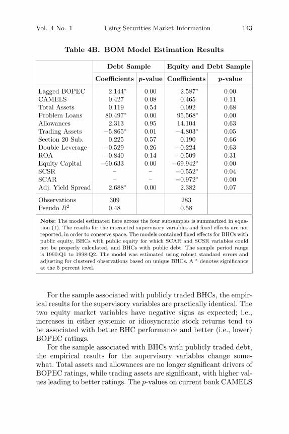
Vol. 4 No. 1 Using Securities Market Information 143
Table 4B. BOM Model Estimation Results
Debt Sample Equity and Debt Sample
Coefficients p-value Coefficients p-value
Lagged BOPEC 2.144∗ 0.00 2.587∗ 0.00CAMELS 0.427 0.08 0.465 0.11Total Assets 0.119 0.54 0.092 0.68Problem Loans 80.497∗ 0.00 95.568∗ 0.00Allowances 2.313 0.95 14.104 0.63Trading Assets −5.865∗ 0.01 −4.803∗ 0.05Section 20 Sub. 0.225 0.57 0.190 0.66Double Leverage −0.529 0.26 −0.224 0.63ROA −0.840 0.14 −0.509 0.31Equity Capital −60.633 0.00 −69.942∗ 0.00SCSR – – −0.552∗ 0.04SCAR – – −0.972∗ 0.00Adj. Yield Spread 2.688∗ 0.00 2.382 0.07
Observations 309 283Pseudo R2 0.48 0.58
Note: The model estimated here across the four subsamples is summarized in equa-tion (1). The results for the interacted supervisory variables and fixed effects are notreported, in order to conserve space. The models contained fixed effects for BHCs withpublic equity, BHCs with public equity for which SCAR and SCSR variables couldnot be properly calculated, and BHCs with public debt. The sample period rangeis 1990:Q1 to 1998:Q2. The model was estimated using robust standard errors andadjusting for clustered observations based on unique BHCs. A ∗ denotes significanceat the 5 percent level.
For the sample associated with publicly traded BHCs, the empir-ical results for the supervisory variables are practically identical. Thetwo equity market variables have negative signs as expected; i.e.,increases in either systemic or idiosyncratic stock returns tend tobe associated with better BHC performance and better (i.e., lower)BOPEC ratings.
For the sample associated with BHCs with publicly traded debt,the empirical results for the supervisory variables change some-what. Total assets and allowances are no longer significant drivers ofBOPEC ratings, while trading assets are significant, with higher val-ues leading to better ratings. The p-values on current bank CAMELS

144 International Journal of Central Banking March 2008
ratings and ROA increase beyond the 5 percent significance level.However, lagged BOPEC ratings, problem loans, and equity capi-tal remain important explanatory variables. For the adjusted yieldspread variable, the positive sign is also in line with expectations;i.e., higher yield spreads relative to the corresponding yield indexare associated with worse BHC performance and worse (i.e., higher)BOPEC ratings.16 The empirical results of the sample for BHCswith both types of publicly traded securities are quite similar tothose of the debt sample. Notably, the adjusted yield spread has apositive coefficient with a p-value of 7 percent, just outside of ourdefined significance level.
These in-sample results clearly suggest that securities marketsprovide information complementary to that generated by supervi-sors. Interestingly, the results for BHCs with both public equity anddebt seem to suggest that equity market variables may be more use-ful than debt market variables. In the next subsection, we examinemore directly the relative importance of these two sources of marketinformation.
3.3 The Relative Importance of Equity and DebtMarket Information
As noted in the introduction, a primary motivation for using bothequity and debt market data in a supervisory monitoring model isthat no single information source is likely to dominate the other inall states of the world. How, then, might these two types of secu-rities market information differ? In which states of the world arethe different sources of information most useful? We might expectthat the residual claim feature of equity implies that equity mar-ket investors would be good at predicting BOPEC rating changeswhen BHC asset values are relatively far from the default point. For
16We estimated versions of the models above that allowed the coefficients onsecurities market variables to differ according to whether the market might per-ceive the institution to be “too big to fail.” For this analysis, we classified a BHCas possibly being too big to fail if it was one of the five largest BHCs by assets in agiven year. We found that equity market prices have the same explanatory valuefor BOPEC ratings for this class of BHCs as for the rest of the sample. Debtprices for the largest BHCs were considerably less useful for signaling changesin condition, although this effect was not measured precisely. Results from thisrobustness check are available from the authors upon request.

Vol. 4 No. 1 Using Securities Market Information 145
such total asset values, changes in value correspond one-to-one withchanges in equity value. Debt market investors, by contrast, mightbe more likely to predict BOPEC rating changes when asset val-ues are relatively close to or below the default point, as that rangefor asset values is where bondholders are most at risk for takinglosses.
To examine the relationship between securities market signalsand how close a BHC might be to default, we explicitly calculate adefault point for each public BHC at each point in time and examinehow its interaction with the securities market variables affects thesupervisory ratings. For this exercise, we use the Ronn-Verma (1986)model for estimating the value of a firm’s assets. Given assumptionson the stochastic process describing changes in asset value, the firm’sequity is modeled as a call option on those assets. This frameworkgives rise to a distance-to-default (DTD) measure, which is the dif-ference between the estimated market value of the assets and theequity, scaled by estimated standard deviation of the rate of returnon the assets. Note that the construction of this measure restrictsour sample to public BHCs.
Working again with ordered logit models within the BOM frame-work, we create indicator variables for whether a BHC’s DTD meas-ure is within a certain percentile of the overall sample distribution ofDTD measures. We constructed nine indicator variables correspond-ing to the first nine deciles of the DTD measure’s unconditionaldistribution. We then interact each indicator variable with the secu-rities market variables to generate nine sets of regression results. Tofocus the analysis, we use a more parsimonious model that has thelagged BOPEC rating as the only supervisory variable; i.e.,
BP∗it = βBPit−2 + (π + αnInit−1)zit−1 + εit , (7)
where zit−1 is the securities market variable in question and Init−1is equal to one if BHC i’s DTD measure is in the nth percentileat time t − 1, and zero otherwise. Our main object of interest iswhether the coefficients on the securities market variables are differ-ent in magnitude depending on how close the BHC is to its defaultpoint.
The estimation results for the 1,291 BOPEC ratings for BHCswith publicly traded equity are presented in table 5A. For the SCAR

146 International Journal of Central Banking March 2008
Table 5A. Estimation Results for the Simplified RatingModel Using DTD Interactions with SCARs
αn
π for InteractionDTD SCAR with DTDPctile. Variable p-value Measure p-value π + αn p-value Pseudo R2
10th Pctile. −0.421 0.00 0.137 0.48 −0.284 0.14 0.3120th Pctile. −0.406 0.00 0.022 0.89 −0.384 0.01 0.3130th Pctile. −0.423 0.00 0.054 0.71 −0.369 0.00 0.3140th Pctile. −0.431 0.00 0.058 0.67 −0.373 0.00 0.3150th Pctile. −0.418 0.00 0.030 0.84 −0.388 0.00 0.3160th Pctile. −0.313 0.00 −0.114 0.42 −0.427 0.00 0.3170th Pctile. −0.271 0.04 −0.155 0.32 −0.426 0.00 0.3180th Pctile. −0.286 0.09 −0.126 0.49 −0.412 0.00 0.3190th Pctile. −0.197 0.41 −0.214 0.40 −0.411 0.00 0.31
Note: The coefficient estimates presented here are for the regression in equation (9). Thesecurities market variable of interest is the BHC SCAR as used previously. The interactedindicator variable is equal to one if the BHC’s distance-to-default (DTD) measure is in thenth percentile of its unconditional distribution. All models are estimated with a sampleof 1,291 observations.
variable described previously, we expect its aggregate coefficientto be negative, suggesting that an increased SCAR that reflectsimproved BHC condition should lead to a better BOPEC rating. Weexpect the disaggregated π coefficient to be negative across all nineregressions. We expect the αn coefficient to have its largest impactfor the lowest DTD percentiles; i.e., the stock market signals forBHCs relatively closer to their default point should be less clear forsupervisory purposes. As shown in the table, the estimated π coeffi-cients are invariably negative and statistically significant for all butthe ninetieth DTD percentile. The αn coefficients are estimated tobe positive for closer-to-default deciles and become negative as thedefault decile is increased, but they are not significantly differentfrom zero. Taken as a whole, the equity market impact measured asthe π + αn values is negative, statistically significant for all but thetenth percentile specification, and in a relatively narrow range. Thus,as expected, equity market signals are weakest for BHCs relativelyclose to the default point.
In table 5B, the zit−1 variable is the adjusted BHC yield spread.The regressions are based on 283 BOPEC ratings assigned to BHCs

Vol. 4 No. 1 Using Securities Market Information 147
Table 5B. Estimation Results for the Simplified RatingModel Using DTD Interactions with the Adjusted
Yield Spreads
π for αn
Adj. InteractionDTD Yield with DTDPctile. Spread p-value Measure p-value π + αn p-value Pseudo R2
10th Pctile. 0.626 0.56 8.906 0.00 9.532 0.00 0.3920th Pctile. 0.245 0.86 1.445 0.56 1.690 0.42 0.3930th Pctile. 1.180 0.55 −0.651 0.77 0.529 0.61 0.3940th Pctile. 1.956 0.22 −1.726 0.36 0.230 0.82 0.3950th Pctile. 2.894 0.01 −3.099 0.05 −0.205 0.85 0.4060th Pctile. 1.646 0.16 −1.095 0.54 0.551 0.66 0.3970th Pctile. 1.859 0.21 −1.315 0.52 0.544 0.66 0.3980th Pctile. 0.116 0.06 0.733 0.76 0.849 0.46 0.3990th Pctile. −1.631 0.50 2.499 0.33 0.868 0.43 0.39
Note: The coefficient estimates presented here are for the regression in equation (9). Thesecurities market variable of interest is the BHC adjusted yield spread as used previously.The interacted indicator variable is equal to one if the BHC’s distance-to-default (DTD)measure is in the nth percentile of its unconditional distribution. All models are estimatedwith a sample of 283 observations.
with both public equity and debt. For this variable, we expect theπ coefficients to be positive, such that an increase in adjusted yieldspreads suggests a worsening of BHC condition and probably a wors-ening of the BOPEC rating. We expect the αn coefficients to bedecreasing and diminishing the overall impact of the market signalas the DTD measure increases; i.e., the debt market signal shouldbe strongest for BHCs closer to their default points. In the table, weshow that, in fact, the coefficient of the estimated (π + α1) coeffi-cient for the percentile closest to the default point is more than fourtimes larger than the coefficients on the other percentiles. Further-more, that first coefficient is the only one that is statistically sig-nificant, due to the statistical significance of the α1 coefficient. Theαn coefficients for the higher DTD percentiles are not statisticallysignificant.
In summary, our simplified ordered logit models suggest an asym-metric contribution of equity and debt market signals to explain-ing BOPEC ratings, and the asymmetry depends on how close theBHC is to its default point. The impact of the equity market signals

148 International Journal of Central Banking March 2008
(π + αn) is largest in magnitude for the BHCs further from default,while the impact of the adjusted yield spreads is much larger inmagnitude for BHCs very close to default.17 These results are inline with theoretical expectations as well as prior empirical research.In particular, they provide further empirical insight into the findingby Berger, Davies, and Flannery (2000) that supervisory and debt-related assessments of BHCs are related. Furthermore, the resultsprovide a refinement of their finding that supervisory and equitymarket assessments are not interrelated; that is, abnormal stockreturns provide useful information with respect to changes in super-visory assessments only for BHCs further from default.
4. Out-of-Sample Forecast Performance
While the BOM model’s in-sample fit and inference is interestingand important, a stricter test of its usefulness for supervisory pur-poses is its out-of-sample forecast accuracy. As in Krainer and Lopez(2003, 2004), we propose to estimate our model over rolling, four-quarter sample periods and evaluate their out-of-sample forecastperformance. Clearly, the number of BOPEC ratings assigned withthese rolling subsamples will be small relative to the full sample, butwe accept the smaller estimation samples in order to simulate howsecurities market data might be used in practice by supervisors.18
However, a major difficulty in applying this forecasting approachto the four BOM models discussed in section 3 is that the numberof observations in any given rolling subsample could be too smallfor the models with securities market data. That is, the numberof BHCs with publicly traded securities within a given forecasting
17This result regarding adjusted BHC yield spreads seems to be consistent withHanweck and Spellman (2002), who found that BHC subordinated debt yieldswere sensitive to solvency concerns if investors’ forbearance expectations (i.e.,time to closure or default) were less than one year.
18The need for four quarters of prior data also causes us to lose some ofthe early BOPEC assignments, mainly because we do not have bond marketdata prior to 1990. The sample used in the forecasting exercise consists of 2,878BOPEC assignments. In this sample there were 638 upgrades, 331 downgrades,and 1,909 no-change inspections corresponding to 509, 290, and 866 unique BHCs,respectively.
Vol. 4 No. 1 Using Securities Market Information 149
window may be too small to permit model estimation. This is par-ticularly true for the two samples of BHCs with publicly tradeddebt. To address this issue, we propose to pool the data and esti-mate a single model using a technique outlined in Griliches (1986).The underlying assumption to justify this pooling is that all rat-ings are generated by the same underlying process. In other words,for the equity sample, publicly traded BHCs are allowed to be dif-ferent from private BHCs, but these differences are assumed to beobservable. Thus, the relationship between a variable—say, the capi-tal ratio—and the BOPEC rating is the same across publicly tradedand private BHCs, holding the other covariates in the model fixed.If this assumption is satisfied, then we can treat the absence of avariable—say, stock market returns for BHCs that are not publiclytraded—as though it were simply a case of missing data. We can thenreplace the missing values with the in-sample mean of the stock mar-ket return variable and estimate the model in equation (2) on thepooled sample, including fixed effects for the observations whereverwe make this data adjustment. Formally, the estimation equationbecomes
BP∗it = βxit−2 + πzit−1 + IEit−1 + IDit−1 + εit , (8)
where the indicator variables IE and ID take on the value of 1 ifBHC i has publicly traded equity and debt, respectively.
This estimation approach has two advantages. First, the coef-ficient estimates on the securities market variables should not beaffected, since we are simply replacing the missing values with thevariables’ mean. Second, the pooling should allow us to get moreefficient estimates of the coefficients on the supervisory variablesbecause we can use all available observations.
To confirm that this procedure does not impact the empiri-cal results, we conducted two robustness tests. First, we checkedwhether the distribution of BOPEC ratings for publicly tradedBHCs differed from that of private BHCs. On average, we foundno statistical differences, suggesting that the subsamples based onpublic equity and/or debt are not markedly different from the wholesample with respect to assigned BOPEC ratings. Second, we com-pared the in-sample estimation results in tables 4A and 4B withthose corresponding to the appropriate specification of equation (8)
150 International Journal of Central Banking March 2008
using the Griliches adjustment. For example, for the case of theequity BOM model, we compare the in-sample estimation resultsbased on the sample of 1,291 inspections of BHCs with publiclytraded equity to the results where we use the full sample of inspec-tions and plug in the mean abnormal return values for BHCs with nostock return data. Table 6 shows that the estimates for the securitiesmarket variables are very similar. The largest difference is observedfor the sample based on BHCs with both public equity and debt,as expected, since it has the smallest sample size. However, evenhere, the coefficients’ signs and significance are similar across theestimation methods. Given that the Griliches adjustment does notalter our results markedly and permits us to conduct our forecastingexercise for all four ratings samples, our forecasting results presentedbelow are based on estimating equation (8) across our rolling datasubsamples using the Griliches adjustment.19
4.1 Forecasting Results
Our measure of whether a model forecasts well is to ask how often itsdirectional forecasts are correct. For example, if the model generatesa signal suggesting a BOPEC upgrade, what percentage of the timedoes an upgrade actually take place? For our purposes, we generatea forecasted BOPEC rating B̂Pit as follows:
B̂Pit =5∑
j=1
j ∗ P̂r(BPit = j), (9)
where P̂r(BPit = j) is the ordered logit model’s forecasted probabil-ity based on information at time t − 1 that BHC i will be assigneda rating of j at time t. We then compare these forecasted ratingsto BPit−1, the ratings as of time t − 1. An upgrade (or downgrade)signal is generated when the forecasted rating is a full rating bet-ter (or worse) than the existing rating. That is, an upgrade sig-nal is given when BPit−1 − B̂Pit ≥ 1, and a downgrade signal is
19In addition, we performed a third robustness check by conducting the out-of-sample exercise for the equity BOM model based on both adjusted and unadjusteddata. Comparisons of these two sets of forecasts are both qualitatively and quan-titatively similar. The results from these robustness checks are available from theauthors upon request.

Vol. 4 No. 1 Using Securities Market Information 151
Tab
le6.
Coeffi
cien
tEst
imat
eson
the
Sec
uri
ties
Mar
ket
Var
iable
sfo
rth
eSubsa
mple
and
Gri
lich
esA
dju
stm
ent
Est
imat
ion
Tec
hniq
ues
Equity
Only
Deb
tO
nly
Equity
and
Deb
t
Subsa
mple
Gri
lich
esSubsa
mple
Gri
lich
esSubsa
mple
Gri
lich
esEst
imat
ion
Adju
stm
ent
Est
imat
ion
Adju
stm
ent
Est
imat
ion
Adju
stm
ent
SCSR
−0.
831∗
−0.
828∗
––
−0.
972∗
−0.
804∗
SCA
R−
0.52
3∗−
0.52
9∗–
–−
0.55
2∗−
0.52
2∗
Adj
.Y
ield
Spre
ad–
–+
2.68
6∗+
2.38
7∗+
2.38
2+
2.23
4∗
Sam
ple
Size
1,29
13,
010
309
3,01
028
33,
010
Note
:A
∗re
pres
ents
sign
ifica
nce
atth
e5
per
cent
leve
l.
152 International Journal of Central Banking March 2008
given when BPit−1 − B̂Pit ≤ −1. A “no change” signal occurs when|BPit−1 − B̂Pit | < 1. Note that we only generate one-quarter-aheadforecasts, even though we evaluate them at various horizons.
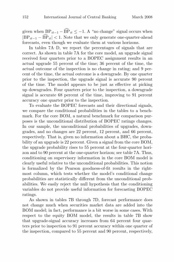
In tables 7A–D, we report the percentages of signals that arecorrect. As shown in table 7A for the core model, an upgrade signalreceived four quarters prior to a BOPEC assignment results in anactual upgrade 55 percent of the time; 36 percent of the time, theactual outcome of the inspection is no change in rating; and 9 per-cent of the time, the actual outcome is a downgrade. By one quarterprior to the inspection, the upgrade signal is accurate 90 percentof the time. The model appears to be just as effective at pickingup downgrades. Four quarters prior to the inspection, a downgradesignal is accurate 68 percent of the time, improving to 91 percentaccuracy one quarter prior to the inspection.
To evaluate the BOPEC forecasts and their directional signals,we compare the conditional probabilities in the tables to a bench-mark. For the core BOM, a natural benchmark for comparison pur-poses is the unconditional distribution of BOPEC ratings changes.In our sample, the unconditional probabilities of upgrades, down-grades, and no changes are 22 percent, 12 percent, and 66 percent,respectively. That is, given no information about a BHC, the proba-bility of an upgrade is 22 percent. Given a signal from the core BOM,the upgrade probability rises to 55 percent at the four-quarter hori-zon and to 90 percent at the one-quarter horizon; see table 7A. Thus,conditioning on supervisory information in the core BOM model isclearly useful relative to the unconditional probabilities. This notionis formalized by the Pearson goodness-of-fit results in the right-most column, which tests whether the model’s conditional changeprobabilities are statistically different from the unconditional prob-abilities. We easily reject the null hypothesis that the conditioningvariables do not provide useful information for forecasting BOPECratings.
As shown in tables 7B through 7D, forecast performance doesnot change much when securities market data are added into theBOM model; in fact, performance is a bit worse in some cases. Withrespect to the equity BOM model, the results in table 7B showthat upgrade-signal accuracy increases from 64 percent four quar-ters prior to inspection to 91 percent accuracy within one quarter ofthe inspection, compared to 55 percent and 90 percent, respectively,

Vol. 4 No. 1 Using Securities Market Information 153
Table 7A. Out-of-Sample Forecast Performanceof the Core BOM Model
Actual Inspection Outcome
Pearson# Signals Upgrade % No Change % Downgrade % Statistic
Signal at −4 Quarters
Upgrade 22 55% 36% 9%
No change 2,825 22% 67% 11%
Downgrade 31 3% 29% 68% 145.0∗
Signal at −3 Quarters
Upgrade 28 68% 21% 11%
No change 2,820 22% 67% 11%
Downgrade 30 0% 17% 83% 254.3∗
Signal at −2 Quarters
Upgrade 45 80% 13% 7%
No change 2,793 22% 68% 10%
Downgrade 40 0% 10% 90% 460.1∗
Signal at −1 Quarter
Upgrade 60 90% 8% 2%
No Change 2,773 21% 69% 10%
Downgrade 45 0% 9% 91% 624.6∗
Note: This table presents the forecast performance results based on the 2,878 BOPECchange signals from the core BOM model at different horizons. A forecast signal is thedifference between the forecasted BOPEC rating and the previously assigned BOPECrating. Signals greater than one (less than one) are forecasts of upgrades (downgrades),respectively. The figures in bold indicate the outcome expected, conditional on the signal.Percentages in rows may not sum to 100 percent due to rounding. The Pearson goodness-of-fit statistic tests the null hypothesis that the distribution of BOPEC change outcomesconditional on the core model forecasts is not different from the unconditional probabilitiesof BOPEC upgrades (22 percent), no changes (66 percent), and downgrades (12 percent).The statistic is distributed χ2(10). A ∗ denotes significance at the 5 percent level.
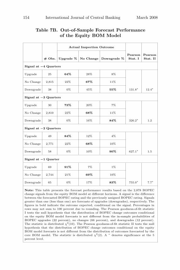
154 International Journal of Central Banking March 2008
Table 7B. Out-of-Sample Forecast Performanceof the Equity BOM Model
Actual Inspection Outcome
Pearson Pearson# Obs. Upgrade % No Change Downgrade % Stat. I Stat. II
Signal at −4 Quarters
Upgrade 25 64% 28% 8%
No Change 2,815 22% 67% 11%
Downgrade 38 0% 45% 55% 131.8∗ 12.4∗
Signal at −3 Quarters
Upgrade 30 73% 20% 7%
No Change 2,810 22% 68% 11%
Downgrade 38 0% 16% 84% 326.2∗ 1.2
Signal at −2 Quarters
Upgrade 49 84% 12% 4%
No Change 2,771 22% 68% 10%
Downgrade 58 0% 10% 90% 627.1∗ 1.5
Signal at −1 Quarter
Upgrade 69 91% 7% 1%
No Change 2,744 21% 69% 10%
Downgrade 65 0% 17% 83% 755.0∗ 7.7∗
Note: This table presents the forecast performance results based on the 2,878 BOPECchange signals from the equity BOM model at different horizons. A signal is the differencebetween the forecasted BOPEC rating and the previously assigned BOPEC rating. Signalsgreater than one (less than one) are forecasts of upgrades (downgrades), respectively. Thefigures in bold indicate the outcome expected, conditional on the signal. Percentages inrows may not sum to 100 percent due to rounding. The Pearson goodness-of-fit statisticI tests the null hypothesis that the distribution of BOPEC change outcomes conditionalon the equity BOM model forecasts is not different from the in-sample probabilities ofBOPEC upgrades (22 percent), no changes (66 percent), and downgrades (12 percent).The statistic is distributed χ2(10). The Pearson goodness-of-fit statistic II tests the nullhypothesis that the distribution of BOPEC change outcomes conditional on the equityBOM model forecasts is not different from the distribution of outcomes forecasted by thecore BOM model. The statistic is distributed χ2(2). A ∗ denotes significance at the 5percent level.

Vol. 4 No. 1 Using Securities Market Information 155
Table 7C. Out-of-Sample Forecast Performanceof the Debt BOM Model
Actual Inspection Outcome
Pearson Pearson# Obs. Upgrade % No Change Downgrade % Stat. I Stat. II
Signal at −4 Quarters
Upgrade 25 52% 40% 8%
No Change 2,818 22% 67% 11%
Downgrade 35 3% 37% 60% 123.1∗ 3.5
Signal at −3 Quarters
Upgrade 27 67% 22% 11%
No Change 2,818 22% 67% 11%
Downgrade 33 0% 21% 79% 246.0∗ 0.9
Signal at −2 Quarters
Upgrade 43 81% 12% 7%
No Change 2,792 22% 68% 10%
Downgrade 43 0% 12% 88% 470.8∗ 1.5
Signal at −1 Quarter
Upgrade 60 88% 8% 3%
No Change 2,765 21% 69% 10%
Downgrade 53 0% 11% 89% 657.2∗ 1.9
Note: This table presents the forecast performance results based on the 2,878 BOPECchange signals from the debt BOM model at different horizons. A forecast signal is thedifference between the forecasted BOPEC rating and the previously assigned BOPECrating. Signals greater than one (less than one) are forecasts of upgrades (downgrades),respectively. The figures in bold indicate the outcome expected, conditional on the signal.Percentages in rows may not sum to 100 percent due to rounding. The Pearson goodness-of-fit statistic I tests the null hypothesis that the distribution of BOPEC change outcomesconditional on the debt BOM model forecasts is not different from the in-sample proba-bilities of BOPEC upgrades (22 percent), no changes (66 percent), and downgrades (12percent). The statistic is distributed χ2(10). The Pearson goodness-of-fit statistic II teststhe null hypothesis that the distribution of BOPEC change outcomes conditional on thedebt BOM model forecasts is not different from the distribution of outcomes forecasted bythe core BOM model. The statistic is distributed χ2(2). A ∗ denotes significance at the 5percent level.

156 International Journal of Central Banking March 2008
Table 7D. Out-of-Sample Forecast Performanceof the Extended BOM Model
Actual Inspection Outcome
Pearson Pearson# Obs. Upgrade % No Change Downgrade % Stat. I Stat. II
Signal at −4 Quarters
Upgrade 28 57% 36% 7%
No Change 2,813 22% 67% 11%
Downgrade 37 0% 43% 57% 126.7∗ 6.4∗
Signal at −3 Quarters
Upgrade 31 68% 267% 6%
No Change 2,808 22% 67% 11%
Downgrade 39 0% 23% 77% 270.5∗ 3.3
Signal at −2 Quarters
Upgrade 48 83% 13% 4%
No Change 2,767 22% 68% 10%
Downgrade 63 0% 13% 87% 633.1∗ 3.1
Signal at −1 Quarter
Upgrade 67 90% 7% 3%
No Change 2,746 21% 69% 10%
Downgrade 65 2% 17% 83% 715.5∗ 11.9∗
Note: This table presents the forecast performance results based on the 2,878 BOPECchange signals from the extended BOM model at different horizons. A forecast signal isthe difference between the forecasted BOPEC rating and the previously assigned BOPECrating. Signals greater than one (less than one) are forecasts of upgrades (downgrades),respectively. The figures in bold indicate the outcome expected, conditional on the signal.Percentages in rows may not sum to 100 percent due to rounding. The Pearson goodness-of-fit statistic I tests the null hypothesis that the distribution of BOPEC change outcomesconditional on the extended BOM model forecasts is not different from the in-sample prob-abilities of BOPEC upgrades (22 percent), no changes (66 percent), and downgrades (12percent). The statistic is distributed χ2(10). The Pearson goodness-of-fit statistic II teststhe null hypothesis that the distribution of BOPEC change outcomes conditional on theextended BOM model forecasts is not different from the distribution of outcomes fore-casted by the core BOM model. The statistic is distributed χ2(2). A ∗ denotes significanceat the 5 percent level.
Vol. 4 No. 1 Using Securities Market Information 157
for the core model. For downgrades, however, forecast performanceimproves from 55 percent to 83 percent as the inspection approaches,which is not quite as large an improvement as for the core model.Overall, the Pearson test results in the last column suggest thatthe addition of the equity market variables does not improve fore-cast performance relative to the core model. In fact, at four quar-ters and one quarter prior, these variables reduce forecast perfor-mance.
In table 7C, the debt BOM model’s forecasting performance isactually a bit worse than that of the core model with only super-visory variables. For example, an upgrade signal four quarters priorto the inspection is correct 52 percent of the time, while a down-grade signal at four quarters prior results in an actual downgrade60 percent of the time. When compared to the core model’s forecastsignals using the Pearson test, we cannot reject the null hypothe-sis that the debt market variables do not improve forecast perfor-mance. Finally, as shown in table 7D, the forecast performance of theextended model with both equity and debt market variables is againmarginally worse than that of the core model. In summary, the intro-duction of securities market variables to the core BOM model failsto improve overall BOPEC forecast performance for rating changesat conventional levels of significance.
4.2 Information in the Forecasts
Although BOPEC change forecasts do not appear to be appreciablydifferent across the core and the extended BOM models presentedin tables 7A–D, the set of BOPEC rating changes correctly sig-naled by these models are not identical. This outcome suggests theneed to think carefully about the cost of forecast errors to supervi-sors. The forecasting literature has shown that combining forecastsfrom different models can improve certain aspects of forecast per-formance; see Granger and Newbold (1986) as well as Diebold andLopez (1996) for further discussion. Hence, another way to gauge thecontribution of securities market information is to examine the addi-tional forecast signals for BHCs with public securities as generatedby the extended models relative to the core model’s signals. Seenin this light, the marginal benefit of monitoring securities marketinformation is notable.

158 International Journal of Central Banking March 2008
Table 8A. Improvements in BOPEC Downgrade Signals
Equity BOM Debt BOM ExtendedModel Model BOM Model
4 Quarters Prior 24% 14% 22%3 Quarters Prior 28% 10% 31%2 Quarters Prior 28% 9% 29%1 Quarter Prior 24% 5% 25%
Note: This table presents the percentage improvement in correct BOPEC down-grade signals when combining the downgrade signals from the core BOM model withthose from the models incorporating securities market data. Downgrade signal isdefined as forecasted rating − current rating > 1. The table reports the number ofdowngrades correctly signaled by the alternative models and not identified by thecore model, expressed as a percentage of downgrades correctly identified by the coremodel. Sample contains 2,878 inspections, with 331 downgrades.
Comparing BOPEC change signals generated by the core andthe three extended BOM models, we ask what is the percentageincrease in the number of correct downgrade signals when securi-ties market data are incorporated into the core BOM model?20 Wefocus on downgrades because these are the events of most interestto supervisors. As reported in table 8A, the extended model withadjusted bond yields and stock return data produces an additional22 percent more correct signals at the four-quarter horizon over andabove those produced by the core model. At the one-quarter hori-zon, the improvement is 25 percent more correct signals. Anotherinteresting point is the similarity between the marginal contribu-tions of the equity BOM model and the extended BOM model withboth equity and debt market variables. Evidently, in this particularframework, most of the additional downgrade signals a supervisorcan extract from securities market data come from the equity mar-ket. This result contrasts with the in-sample results and may be dueto the relatively small number of BHCs with publicly traded debtin any given subsample period.
Of course, these three BOM models also produce incorrect signalsover and above those produced by the core model. Since table 8A
20Note that all of these additional correct forecasts are for ratings changes atBHCs with publicly traded securities.

Vol. 4 No. 1 Using Securities Market Information 159
Table 8B. Trade-Off between Correct and IncorrectDowngrade Signals
Equity BOM Debt BOM ExtendedModel Model BOM Model
4 Quarters Prior 1/2 7/11 11/253 Quarters Prior 17/12 6/7 19/172 Quarters Prior 23/17 7/4 6/51 Quarter Prior 3/2 5/1 5/3
Note: This table presents the trade-off between additional correct and additionalincorrect BOPEC downgrade signals provided by the alternative BOM models rel-ative to the core BOM model. A cell entry of x/y suggests that the alternativeBOM model identifies x additional correct downgrades signals beyond those of thecore model, at the rate of y additional incorrect downgrade signals. Sample contains2,878 inspections, with 331 downgrades.
shows that these models identify additional BOPEC downgrades,their mistakes may be responsible for our earlier result that theiroverall forecast performance was almost the same as the core model.We examine this trade-off more closely in table 8B, where we expressthe models’ ratios of correct downgrade signals to incorrect signals,which are also known as false positives or type 2 errors. For theextended BOM model at the four-quarter horizon, the model pro-duces eleven additional correct signals at the cost of twenty-fiveincorrect downgrade signals. By the one-quarter horizon, however,the performance improves dramatically to five additional correct sig-nals at the cost of only three additional incorrect signals. The modelsextended by equity variables and debt variables alone behave simi-larly.21 Interestingly, this signal trade-off for the debt BOM modelis quite good; by one quarter out, it produces five correct signalsfor every incorrect signal. However, as indicated in table 8A, the
21Gropp, Vesala, and Vulpes (2004, 2006) conduct a similar analysis, but theyfocus on in-sample model fit. In their analysis, incorporating securities marketvariables into their model reduces false positive errors (i.e., type 2 errors). Ourresults align well with this result in that the combination of BOPEC downgradesignals from the core BOM model with the three expanded models adds morecorrect than incorrect signals, especially nearer to the BOPEC assignment; i.e.,the combined set of signals has a reduced type 2 error rate than the set basedjust on the core model.

160 International Journal of Central Banking March 2008
drawback to this model is that it produces relatively fewer signalsbeyond those from the core model.
In summary, our analysis of combined BOPEC downgrade signalsindicates that models using securities market data can generate areasonably large number of additional correct downgrade signals rel-ative to the core BOM model. Given the emphasis placed by super-visors on BOPEC downgrades, we believe that these forecastingresults argue for closer monitoring of securities market informationfor off-site supervisory monitoring.
5. Conclusion
Our empirical results indicate that both equity and debt marketinformation are useful in improving the in-sample fit of our pro-posed BOM model for BOPEC ratings. Both types of securitiesmarket information also appear to be useful in explaining BOPECupgrades and downgrades. Moreover, for our data set, we detect non-linearities in the impact of securities market variables on BOPECratings. For BHCs closer to their estimated default points, the effectof our adjusted BHC bond yield spreads on BOPEC ratings islarger in magnitude than it is for BHCs further from their defaultpoints, and vice versa for equity market data. These results pro-vide further empirical support for the finding by Berger, Davies,and Flannery (2000) that supervisory and debt-related assessmentsof BHCs are correlated and a refinement of their finding thatsupervisory and equity market assessments are not related; i.e.,abnormal BHC stock returns provide useful information regardingsupervisory assessments for BHCs that are far from their defaultpoints.
When we turn to out-of-sample forecasting, however, evidencefor the usefulness of market information is disappointingly weak.For our analysis, we estimate our four BOM model specifications ona rolling subsample of data and then forecast BOPEC ratings out ofsample. We find the forecast performance of the three BOM modelsthat include securities market data is not much different than theperformance of the core model based on supervisory data alone.
While the overall forecasting performance of the four BOM mod-els is similar, the sets of forecasted rating changes are not identical.That is, the core model correctly identifies one set of BOPEC rating

Vol. 4 No. 1 Using Securities Market Information 161
changes, particularly downgrades, while the extended models cor-rectly identify other sets of downgrades. The extended BOM modelscorrectly identify additional BOPEC downgrades for publicly tradedBHCs over and above the correct forecasts from the core model.These additional correct forecasts can be achieved at a relativelymodest cost of additional incorrect signals. Hence, supervisory useof securities market information within the context of an off-sitemonitoring model, such as our proposed BOM model, appears to bereasonable.
References
Basel Committee on Banking Supervision. 2003. “Markets for BankSubordinated Debt and Equity in Basel Committee MemberCountries.” Working Paper No. 12, Bank for InternationalSettlements.
Berger, A. N., S. M. Davies, and M. J. Flannery. 2000. “ComparingMarket and Supervisory Assessments of Bank Performance: WhoKnows What When?” Journal of Money, Credit, and Banking32 (3): 641–67.
Bliss, R., and M. Flannery. 2001. “Market Discipline in the Gov-ernance of U.S. Bank Holding Companies: Monitoring ver-sus Influencing.” In Prudential Supervision: What Works andWhat Doesn’t, ed. F. S. Mishkin, 107–43. Chicago: University ofChicago Press.
Board of Governors of the Federal Reserve System. 1999. “UsingSubordinated Debt as an Instrument of Market Discipline.”Report of the Study Group on Subordinated Notes and Deben-tures. Federal Reserve System Staff Study No. 172.
———. 2004. “Bank Holding Company Rating System.” Supervisionand Regulation Letter No. 04-18, Division of Banking Supervi-sion and Regulation.
Campbell, J. Y., A. W. Lo, and A. C. MacKinlay. 1997. The Econo-metrics of Financial Markets. Princeton, NJ: Princeton Univer-sity Press.
Cole, R. A., and J. W. Gunther. 1998. “Predicting Bank Failures: AComparison of On- and Off-Site Monitoring Systems.” Journalof Financial Services Research 13 (2): 103–17.

162 International Journal of Central Banking March 2008
Covitz, D. M., D. Hancock, and M. L. Kwast. 2004a. “A Reconsider-ation of the Risk Sensitivity of U.S. Banking Organization Subor-dinated Debt Spreads: A Sample Selection Approach.” EconomicPolicy Review (Federal Reserve Bank of New York) 10 (2): 73–92.
———. 2004b. “Market Discipline in Banking Reconsidered:The Roles Funding Manager Decisions and Deposit InsuranceReform.” Finance and Economics Discussion Series No. 2004-53,Board of Governors of the Federal Reserve System.
DeFerrari, L. M., and D. E. Palmer. 2001. “Supervision of LargeComplex Banking Organizations.” Federal Reserve Bulletin(February): 47–57.
DeYoung, R., M. J. Flannery, W. W. Lang, and S. M. Sorescu. 2001.“The Information Content of Bank Exam Ratings and Subor-dinated Debt Prices.” Journal of Money, Credit, and Banking33 (4): 900–25.
Diebold, F. X., and J. A. Lopez. 1996. “Forecast Evaluation andCombination.” In Handbook of Statistics 14: Statistical Methodsin Finance, ed. G. S. Maddala and C. R. Rao, 241–68. Amster-dam: North-Holland.
Estrella, A., S. Park, and S. Peristiani. 2000. “Capital Ratios asPredictors of Bank Failure.” Economic Policy Review (FederalReserve Bank of New York) 6 (2): 33–52.
Evanoff, D., and L. Wall, L. 2001. “Sub-debt Yield Spreads as BankRisk Measures.” Journal of Financial Services Research 20 (2):121–46.
———. 2002. “Measures of the Riskiness of Banking Organizations:Subordinated Debt Yields, Risk-Based Capital and ExaminationRatings.” Journal of Banking and Finance 26 (5): 989–1009.
Flannery, M. J. 1998. “Using Market Information in Prudential BankSupervision: A Review of the U.S. Empirical Evidence.” Journalof Money, Credit, and Banking 30 (3): 273–305.
Flannery, M. J., and S. U. Sorescu. 1996. “Evidence of Bank Mar-ket Discipline in Subordinated Debenture Yields: 1983–1991.”Journal of Finance 51 (4): 1347–77.
Goyal, V. K. 2005. “Market Discipline of Bank Risk: Evidence fromSubordinated Debt Contracts.” Journal of Financial Intermedi-ation 14 (3): 318–50.
Granger, C. W. J., and Newbold, P. 1986. Forecasting EconomicTime Series. 2nd ed. San Diego: Academic Press.
Vol. 4 No. 1 Using Securities Market Information 163
Griliches, Z. 1986. “Economic Data Issues.” In Handbook of Econo-metrics, Vol. III, ed. Z. Griliches and M. D. Intriligator. Amster-dam: Elsevier Science Publishers BV.
Gropp, R., and A. J. Richards. 2001. “Rating Agency Actions andthe Pricing of Debt and Equity of European Banks: What CanWe Infer About Private Sector Monitoring of Bank Soundness?”Economic Notes 30 (3): 373–98.
Gropp, R., J. Vesala, and G. Vulpes. 2004. “Market Indicators, BankFragility, and Indirect Market Discipline.” Economic Review(Federal Reserve Bank of New York) 10 (2): 53–62.
———. 2006. “Equity and Bond Market Signals as Leading Indica-tors of Bank Fragility.” Journal of Money, Credit, and Banking,38 (2): 399–428.
Gunther, J. W., and R. R. Moore. 2003. “Early Warning Models inReal Time.” Journal of Banking and Finance 27 (10): 1979–2002.
Hancock, D., and M. Kwast. 2001. “Using Subordinated Debt toMonitor Bank Holding Companies: Is It Feasible?” Journal ofFinancial Services Research 20 (2): 147–87.
Hanweck, G. A., and L. J. Spellman. 2002. “Forbearance Expec-tations and the Subordinated Debt Signal of Bank Insolvency.”Manuscript, School of Management, George Mason University.
Hirtle, B. J., and J. A. Lopez. 1999. “Supervisory Information andthe Frequency of Bank Examinations.” Economic Policy Review(Federal Reserve Bank of New York) 5 (1): 1–20.
Krainer, J., and J. A. Lopez. 2003. “How Might Financial Mar-ket Information Be Used for Supervisory Purposes?” EconomicReview (Federal Reserve Bank of San Francisco), 29–45.
———. 2004. “Incorporating Equity Market Information into Super-visory Monitoring Models.” Journal of Money, Credit, and Bank-ing 36 (6): 1043–67.
Meyer, P. A., and H. W. Pifer. 1970. “Prediction of Bank Failures.”Journal of Finance 25 (4): 853–68.
Pettway, R. H., and J. F. Sinkey. 1980. “Establishing On-SiteBank Examination Priorities: An Early-Warning System UsingAccounting and Market Information.” Journal of Finance 35 (1):137–50.
Ronn, E. I., and A. K. Verma. 1986. “Pricing Risk-Adjusted DepositInsurance: An Option-Based Model.” Journal of Finance 41 (4):871–95.

164 International Journal of Central Banking March 2008
Sahajwala, R., and van den Bergh, P. 2000. “Supervisory RiskAssessment and Early Warning Systems.” Basel Committee onBanking Supervision Working Paper No. 4, Bank for Interna-tional Settlements.
Sinkey, J. F. 1975. “A Multivariate Statistical Analysis of the Char-acteristics of Problem Banks.” Journal of Finance 30 (1): 21–36.


![Securities Market [Finance]](https://img.pdfslide.us/doc/110x75/577d20ee1a28ab4e1e941055/securities-market-finance.jpg)