1

USING SCATS DATA TO PREDICT BUS TRAVEL TIME

Ehsan Mazloumi, Graham Currie, Geoff Rose, and Majid Sarvi Institute of Transport Studies, Monash University, Melbourne, Australia

ABSTRACT

The provision of accurate travel time information of public transport vehicles is valuable for both operators and passengers. It helps operators effectively implement their management strategies. It also allows passengers to schedule their departure to minimize waiting times. Public transport travel time is affected by several factors such as traffic flow, passenger demand, etc, which have to be considered to make precise predictions. However, previous studies have not explicitly considered real world traffic flow variables in their prediction models.

This paper aims at using traffic flow data to predict bus travel time, and at examining the value which traffic flow data could make to the accuracy of predictions. It uses travel time values obtained from GPS recorded data from a bus route in Melbourne, Australia, to develop three models. The first model is an artificial neural network that uses saturation degree data collected by the Sydney Coordinated Adaptive Traffic System (SCATS) at intermediate signalized intersections along with schedule adherence to predict bus travel time. A historical data based neural network that uses temporal variables (time of day, day of week and month of year) and schedule adherence as well as a model that traditionally utilizes scheduled travel times for future travel time predictions are also developed. The results show that the first model outperforms other models.

1 INTRODUCTION

The provision of accurate arrival time predictions of on-road public transport vehicles (e.g. buses) is valuable for both operators and passengers. With this information, in the short term, operators can effectively mitigate disruptions in scheduled arrival times or headways by applying real time management strategies such as holding and stop skipping (Osuna and Newell 1972; Fu and Yang 2002; Fu et al. 2003). The long term benefit would be to use arrival time prediction models for off-line planning and design purposes including fleet size planning, schedule design, and passenger travel time performance assessment (Ceder 2007; Mishalani et al. 2008).

Arrival time information also benefits passengers by helping them efficiently schedule their departure times, and successfully make transfers at transit stations. These will enhance service quality by reducing passengers‟ waiting times and their anxiety, and will attract more ridership.

Bus travel time is affected by several factors such as traffic flows at intersections, passenger demand at stops, and weather conditions (Chen et al. 2004), which have to be taken into account to make precise predictions. However, existing studies have not explicitly considered real world traffic flow measures in predicting travel times. Therefore, they may not be able to effectively consider the effect of varying traffic states in their predictions.

This paper aims at using the Sydney Coordinated Adaptive Traffic System (SCATS) data to predict bus travel time, and at examining the value which traffic flow data would make to the accuracy of predictions. Six month travel time values obtained from a bus route in Melbourne, Australia, were used to develop three models. The “traffic flow data based” model uses saturation degree data collected by the SCATS at intermediate signalized intersections to predict bus travel time. Since collecting traffic flow data is not always an easy task, the other developed models have input values that are easier to collect. A “historical data based” model that uses temporal variables (time of day, day of week and month of year) as well as a “traditional model” that utilizes scheduled travel times for future travel time

2

predictions are developed. Other variables including weather conditions and schedule adherence are also examined for their inclusions in the models.

The paper first reviews the existing approaches to predict bus arrival time. The data used in this paper are then explained, followed by steps to develop the study models, and a comparison of different model performances. A closing summary, conclusions, and suggestions for future research are included in the final section of the paper.

2 LITERATURE REVIEW

With the emergence of Advanced Public Transportation Systems (APTS) such as Global Position Systems (GPS), Automatic Vehicle Location (AVL) and Automatic Passenger Counting (APC) systems, using these systems to predict transit arrival/travel time has been a challenging problem. While several studies have been directed to address this problem, adopted methodologies may be generally grouped into four categories: (a) regression models, (b) Artificial Neural Network (ANN) models, (c) Kalman filter models, and (d) analytical approaches.

Regression models establish a mathematical relationship between a dependent variable, i.e. bus arrival/travel time, and independent variables such as section length, number of intermediate bus stops, number of signalized intersections, weather conditions, etc. Abdelfattah and Khan (1998) used simulation data to develop several linear and non-linear regression models to predict bus delay in normal conditions as well as when one traffic lane is blocked. Patnaik et al. (2004) also developed a set of regression models to estimate bus arrival times to downstream stops with data collected by APC systems. The main disadvantage of regression models is their requirement to a set of uncorrelated independent variables. However, in many applications, independent variables are correlated to each other, and the provision of such these variable sets is not an easy task.

ANN models can explain complex and non-linear relationships between a variable and a set of explanatory variables through adjusting their parameters (Hagan et al. 1995). ANN input values (explanatory variables) do not need to be uncorrelated. In addition, ANNs do not need the mathematical form of relationships as needed by regression models. The complex relationship between bus arrival/travel time and its determinants have been determined by ANNs adopted by several studies. Kalaputapu and Demetsky (1995) used AVL data to explore the ability of ANNs to predict bus schedule deviation at each stop. Jeong and Rilett (2004) used AVL data to develop ANNs to predict bus travel times from each particular bus stop to downstream bus stops. Their ANN outperformed historical and regression models. Other examples of studies adopted ANNs include (Park et al. 2004) and (Chen et al. 2007).

The Kalman filter is a linear recursive predictive algorithm used to estimate the parameters of a process model. It starts with a primary estimate and allows parameters to be adjusted with each new measurement (Kalman 1960). Unlike regression and ANN models that are calibrated based on historical data, the Kalman filter can respond to dynamic conditions of a modelled process, which is why it has been used for dynamic travel time prediction models. Chien et al. (2002) worked with simulation data to enhance the performance of ANN models in dynamic applications. The arrival time to each bus stop was predicted by an ANN as a function of simulation data such as link speed, link traffic flow, link density, etc. A Kalman filter then modified the arrival time of each bus by considering the arrival time prediction error of the previous bus to that bus stop. Shalaby and Farhan (2004) used five weekdays of data from AVL and APC systems to predict bus arrival time by integrating two Kalman filters. The first filter predicted travel time between each two consecutive timing points from historical travel times, whereas the other filter predicted passenger arrival rate at a timing point based on historical passenger rates. The dwell time was then calculated based on the predicted passenger arrival rate and headway. Chen et al. (2004) used Kalman filter to improve the prediction error of ANN models. Prior to the start of each trip, the ANN models predicted travel times between an origin and all downstream bus stops. Then, when the bus reached a bus stop, the arrival time recorded by an APC system

3

was used by a Kalman filter to update arrival time predictions to downstream bus stops. Kalman filter was also used by Dailey et al. (2001) to predict arrival time from historical trajectory data, and by Chen et al. (2005) to predict arrival time with taking into account the effect of schedule recovery impact.

Several studies used APTS data to implement analytical approaches to predict transit vehicle travel/arrival time. However, these approaches were developed based on specific available data or special conditions of each study. Lin and Zeng (1999) used GPS data to develop a mathematical algorithm to provide real time arrival time information for a rural bus service. Bus location data, schedule information, the difference between scheduled and actual arrival time, and waiting time at time-check stops were used as the main model variables. The algorithm was primarily developed for rural areas where traffic congestion is minimal or does not exist. Sun et al. (2007) proposed an algorithm, which consisted of two parts, for using GPS data for bus arrival time prediction. The first component was to track the bus to obtain the distance to each bus stop, whereas the second component predicted bus arrival time using average travel speed in different temporal and spatial segmentations. Other examples may include (Lin and Bertini 2004) that formulated a Markov chain to pursue schedule recovery effect on bus travel time, and (Mishalani et al. 2008) that considered the effect of different characteristics of driver-bus pairs on arrival time prediction.

Table 1 summarizes different studies adopted different methodologies. This Table also presents the variables used to predict bus arrival/travel time in addition to the data source used. As seen, none of the existing studies has used the real world traffic flow data to predict bus travel time.

Table 1: The explanatory variables used in different studies to predict bus arrival/travel time.

Adopted methodology

Study Variables used in prediction Data

source

Regression

Abdelfattah and Khan (1998)

route characteristics, no. of buses per link, traffic density, no. of passengers boarding

Simulation

Patnaik et al. (2004)* length, no. of stops, cumulative dwell time, time

of day variables APC

Neural network

Kalaputabo and Demetsky (1995)

schedule arrival time, schedule deviation AVL

Jeong and Rilett (2004) arrival time, dwell time, schedule adherence AVL

Park et al. (2004)* GPS bus location data GPS

Chen et al. (2007) weather, dwell time, day of week, time of day,

trip pattern APC

Kalman filter

Chien et al. (2002) traffic measures, historical passenger arrival

rate, bus arrival time Simulation

Shalaby and Farhan (2004)

historical travel times, historical passenger arrival rate

AVL - APC

Chen et al. (2004) day of week, time of day, weather, route

section, arrival time at previous stops APC

Dailey et al. (2001) historical trajectory of buses AVL

Chen et al. (2005) schedule travel time, last section travel time AVL - APC

Analytical approach

Lin and Zeng (1999) GPS bus location data, time table, delay GPS

Lin and Bertini (2004) historical trajectory of buses GPS

Sun et al. (2007) GPS bus location, historical average speed GPS

Mishalani et al. (2008) historical arrival/travel times, GPS

* The study developed a bus arrival/travel time estimation model.

4

3 DATA

The test bed for this study is a part of bus route 246 in Melbourne, Australia, starting from Clifton Hill ending at St Kilda junction. Figure 1 is a schematic presentation of this test bed. This site is about eight kilometres in length, which comprises four sections demarcated by five timing point stops including Clifton Hill, Johnston St., Bridge Rd., Toorak Rd., and St Kilda junction. The sections are relatively equal in length, and are located in the inner parts of Melbourne, and they experience a high level of passenger demand and traffic flow especially in peak hours. Bus headways vary from ten minutes in the peak to about half an hour in the off peak hours. In addition, buses operate in mixed traffic without a dedicated bus lane.

Figure 1: A schematic representation of the study test bed.

A selection of buses were equipped with GPS devices, and their arrival/departure times

corresponding to timing points were recorded. A six month travel time dataset of 2007 (starting from February) derived from the GPS recorded dataset was available for the research. This includes about 2,050 travel time observations corresponding to each section between two consecutive timing points. Figure 2 shows the typical distributions of travel time values over two of the sections: Johnston St. to Bridge Rd, and Bridge Rd. to Toorak Rd. Accordingly, over either of the sections, the travel times present a distinct morning peak, whereas in a comparative sense, the afternoon peaks are relatively flatter. As seen in this Figure, the travel time values of each section vary considerably over different days at each time. For example, the travel times at the section Johnston St. to Bridge Rd. at 2:00pm vary over different days from about 200 seconds to about 600 seconds. This might have resulted from a range of factors such as variations in passenger demand and traffic flow over different days as well as various signal delays experienced by different buses, and dissimilar driving behaviour of bus drivers.

Traffic counts and Degree of Saturation (DS) values were recorded by the SCATS loop detectors installed at signalized intersection stop lines. For each section, when a bus started its travel from a timing point towards downstream timing points, for each signalized intersection along the section under study, the average traffic counts and DS values over the previous signal cycles are derived.

Weather conditions can affect bus travel time by influencing drivers‟ performance and vehicle headways (Hofman and Mahony 2005). To explore the effect of weather conditions, the amount of rain (in millimetres) that fell over the corresponding hour is also used in the analysis.

Schedule adherence can affect bus travel time (Mazloumi et al. 2008), so this variable is also examined for inclusion in the prediction. Schedule adherence is quantified by subtracting observed arrival time from scheduled arrival time

5

(a) Johnston St. to Bridge Rd.

(b) Bridge Rd. to Toorak Rd.

Figure 2: Typical distributions of travel times across the day.

4 MODEL DEVELOPMENT

In this study, three models are developed to predict bus travel time corresponding to different sections between each two consecutive timing point stops. The first model, traffic flow data based model uses the SCATS data to predict bus travel time. The historical data based model predicts travel times as a function of temporal variables and the traditional model uses scheduled travel times to predict future travel times. However, when developing the first two models, other variables are also examined for their inclusions in the models.

Following the general approach to examine a model prediction performance, the travel time dataset of each section was divided into two randomly selected datasets: a training dataset (80 percent of data: 1,700 records of input-output values), and a testing dataset (20 percent of data: 350 records of input-output values). Different models corresponding to each section are then trained on the training dataset, and are tested based on the testing dataset.

4.1 Traffic flow data based model

The ANalysis Of VAriance (ANOVA) technique is used to select the model input variables. This technique identifies the variables that best explain the variability in a dependent variable. The dependent variable is bus travel time, and variables whose effects on bus travel times are explored are the SCATS data, weather conditions, and schedule adherence.

6

First, the selection procedure examines the effect of different time window lengths to collect the SCATS data (t1) on the level of variability explained by the different SCATS data. When t1 equals to 15 minutes, the SCATS data of the signal cycles within the previous 15 minutes are taken into account for prediction. The ANOVA examines the SCATS data including traffic counts and DS in different t1. These data are separately taken into account in the ANOVA process to investigate how they explain the variability in the dependent variable, bus travel time. Table 2 reports the portion of the variability explained by each variable in terms of adjusted R2.

Table 2: ANOVA results with traffic counts and DS in different prediction horizons (adjusted R

2).

Section t1

(minute)

Selected explanatory variable**

Traffic count Degree of Saturation

(DS) Traffic count &

DS

With no interaction

With interaction*

With no interaction

With interaction*

With no interaction

With interaction*

Clifton Hill to

Johnston

2 0.47 0.49 0.47 0.50 0.49 0.50

15 0.49 0.51 0.49 0.52 0.50 0.52

30 0.40 0.44 0.41 0.45 0.41 0.46

60 0.30 0.35 0.29 0.35 0.30 0.34

Johnston to

Bridge

2 0.23 0.26 0.29 0.38 0.30 0.38

15 0.25 0.28 0.31 0.39 0.32 0.40

30 0.20 0.23 0.25 0.32 0.26 0.32

60 0.17 0.19 0.21 0.28 0.21 0.29

Bridge to

Toorak

2 0.44 0.47 0.45 0.49 0.46 0.50

15 0.46 0.54 0.47 0.55 0.49 0.55

30 0.43 0.50 0.45 0.51 0.46 0.52

60 0.38 0.45 0.39 0.45 0.40 0.46

Toorak to

St Kilda

2 0.18 0.21 0.19 0.21 0.21 0.22

15 0.20 0.22 0.20 0.22 0.23 0.24

30 0.17 0.18 0.18 0.18 0.18 0.18

60 0.15 0.17 0.16 0.17 0.16 0.17

* Two and three way interaction terms are considered

** The optimal t1 where the SCATS data give the highest adjusted R2 are underlined

The conclusions that could be drawn from Table 2 include:

The analysis uses the DS values to predict bus travel time. This is because considering DS leads to relatively higher values of adjusted R2 than those obtained when traffic count is considered. When DS is used together with traffic count, a minor improvement can be seen in the adjusted R2. In addition, while traffic count describes the fluctuations in demand, using DS ensures capturing variations caused by changes in supply (signal cycle/green time) as well as those in demand.

When predicting travel time, it is important to consider the interaction of input variables as they also contribute in the variation of travel time values.

The highest portion of variability is explained by the SCATS data when t1 is equal to 15 minutes. This suggests that the most accurate predictions can be made when traffic flow data are obtained from the last 15 minute interval prior to the departure of bus from the upstream timing point. In larger intervals, travel time values are less related to the selected variables. Meanwhile, increasing the interval length necessitates recording and storing more data, which do not improve the model

7

performance. In shorter intervals, say 2 minutes, sometimes two signal cycles fall into the interval, while in some other occasions only one signal cycle corresponds to the interval. This causes non-smooth average traffic flow in successive intervals.

The results in this table show that a considerable extent of variability in travel times can not be explained by the selected explanatory variables. For example, for the “Clifton Hill to Johnston” section, only half of the variability is explained when degree of saturation is considered. The un-explained part of the variability might be related to different signal delays and dwell times at stops.

The next step is to examine the effect of schedule adherence and weather condition on

travel time variability. Table 3 reports the results of this investigation through an ANOVA analysis. As seen, when only weather variable is considered, the adjusted R2 is zero, which implies that the weather variable does not contribute to the variability of travel time values in either of the sections. Unlike, schedule adherence associates with positive adjusted R2, which shows the importance of this variable in the variations of dependent variable. Accordingly, the model will use the average DS values over signal cycles embedded in the last 15 minute interval prior to the bus departure from the upstream timing point along with schedule adherence to predict bus travel time.

Table 3: Level of variation in travel time values explained by different variables (adjusted R

2).

Section

Model variables*

Saturation degree**

Weather (rainfall)

Schedule adherence

Saturation degree & schedule adherence

Clifton Hill to Johnston 0.52 0.00 0.02 0.53

Johnston to Bridge 0.40 0.00 0.02 0.42

Bridge to Toorak 0.55 0.00 0.03 0.57

Toorak to St Kilda 0.24 0.00 0.02 0.25

* All two and three way interaction terms are considered ** In the last 15 minute interval prior to the departure of the bus

4.1.1 Model structure

To predict bus travel time of each bus route section, a feed-forward back-propagation neural network is used, whose structure is shown in Figure 3. The inputs are schedule adherence and DS values at different signalized intersections. Each network has one hidden layer neuron since it suffices to closely map any relationship (Jain & Nag 1997). The link weights and biases are the model parameters calibrated though the training process.

The analysis uses sigmoid function in hidden layer neurons, which has shown good convergence properties through it differentiability (Palacharla & Nelson 1999). This function takes the inputs, which may take any value, and map them into the range of 0 and 1. The increasing behaviour of this function to some extents agrees with the obvious relation that travel time increases with traffic flow/saturation degree.

4.1.2 Training method

A batch (or off-line) training approach is used, where parameters are optimized with respect to the entire training dataset. To improve the model generalization over the testing dataset, Bayesian Regularization is used (Bishop 1995). It minimizes a combination of prediction error and weights, and determines the correct combination so that the model generalizes well.

8

4.1.3 Initial parameters

Different initial model parameters may lead to different network outcomes, so initial weights are very important to obtain the optimal solution. To increase the likelihood of obtaining the optimum answer, each neural network is run for 100 times to find the best initial point that leads to the most accurate prediction outcomes.

Figure 3: The study adopted neural network (the Model 1).

4.1.4 Data pre-processing

Input and output values are linearly rescaled before training the network to ensure that all inputs are treated equally in the regularization process (Hastie et al. 2001).

4.1.5 The number of hidden neurons

Determining the number of hidden layer neurons is a trade-off between the model complexity and its generalizing ability. More hidden neurons may empower the model to better describe the relationship between input and output values, which may make the model more prone to over fit the data and hence have poor generalization. On the other hand, a simple model may not have an adequate power to describe all the complexity in the problem under study.

As a conventional approach, this paper adopts a trial and error procedure using different numbers of hidden neurons for each neural network. Table 4 shows how the model outcomes vary when the number of hidden neurons increases from one to ten. For each model with a different hidden layer neuron, the Mean Absolute Relative Error (MARE) is reported, which can be calculated from Equation (1):

M

O oY

oYoY

MMARE

1 )(

)()(1 (1)

where M is the total number of input-output pairs in the testing dataset, )(oY is the observed

travel time value, and )(oY is the corresponding predicted travel time.

Interestingly, for each route section, the model outcomes are not considerably different, and they are not too much sensitive to the number of hidden neurons. For each section under study, the best model results are underlined.

9

Table 4: MARE of testing the neural networks in terms of different number of hidden neurons

Section Number of hidden neurons

1 2 3 4 5 6 7 8 9 10

Clifton Hill to Johnston 21.7 21.8 20.1 22.1 21.0 23.2 20.6 24.2 20.9 20.5

Johnston to Bridge 23.3 19.4 19.6 19.5 19.8 20.2 20.0 19.7 20.1 20.0

Bridge to Toorak 19.2 16.8 17.3 17.2 18.5 19.0 20.0 20.8 19.1 19.0

Toorak to St Kilda 19.0 19.1 18.4 18.5 18.5 18.7 20.6 20.2 18.5 18.4

Note: The nest model results are underlined for each section.

4.2 Historical data based model

The ANOVA technique is also used to determine the input variables of the historical data based model. The dependent variable is bus travel time, and the independent variables are temporal variables and schedule adherence. The weather variable is not considered as its effect on bus travel time was found insignificant during the Model 1 development.

Temporal variables used in the ANOVA analysis are time of day that indicates different 15 minute interval during the day, day-of-week that shows five different weekdays, and month of year that indicates different months of a year. Table 5 reports the contribution of different variables in the variability of different section travel times. Accordingly, time of day variable has the highest impact on the variability of travel time values. The interaction terms also explain a part of variation in travel time values as their inclusion improves the adjusted R2.

Table 5: Level of variation in travel time values explained by different variables (adjusted R

2).

Section Time

Of Day (TOD)

Day Of Week (DOW)

Month Of Year (MOY)

Schedule adherence

TOD, DOW, MOY, and schedule adherence

With out interaction

With interaction*

Clifton Hill to Johnston 0.45 0.02 0.01 0.02 0.50 0.52

Johnston to Bridge 0.35 0.02 0.01 0.02 0.39 0.42

Bridge to Toorak 0.43 0.01 0.01 0.03 0.50 0.52

Toorak to St Kilda 0.18 0.03 0.02 0.02 0.24 0.26

* two and three way interaction terms are considered

For each route section, we adopt an ANN with input values being temporal variables

and schedule adherence. The ANNs are calibrated through the steps explained in the previous section. The optimal structures of the networks are reported in Table 6. For each section, the number of hidden neurons is higher compared to when the DS values are used. This suggests the higher complexity level of the problem when temporal variables are used. This is because temporal variables do not have a direct relationship with travel times, and the model has to understand how the varying variables such as DS values affect travel times in different temporal scales. However, when the DS values are used, the variation in the DS values will be directly presented to the model.

10

Table 6: The number of hidden neurons in different ANNs (Historical data based model).

Route section

Clifton Hill to Johnston

Johnston to Bridge

Bridge to Toorak

Toorak to St Kilda

7 5 7 7

Note: Inputs are temporal variables and schedule adherence

4.3 Traditional model

A traditional approach to predict future travel time is to refer to the timetables and use the scheduled travel times. To predict travel time for each section, the traditional model uses scheduled travel times, which are available from the information given on timetables.

5 RESULTS

The comparison results presented in Table 7 suggest that using the DS values instead of temporal variables will lead to minor improvements in the MARE (except with the “Bridge to Toorak” section). This is because the time to time variation (the variation over a day) of DS is similar over different days, so DS can be relatively well represented by temporal variables. However, when DS values are used, the model can take into account some unexpected variations in DS (which are irrespective to the time of day), which leads to the predictions being more accurate.

Using scheduled travel times to predict future travel time will lead to relatively poor results compared to those obtained from other models. This is because for each time of day, scheduled travel times are almost constant over different days/months. Therefore, they are not able to capture the travel time variations caused by a range of factors. However, at the Johnston to Bridge section, where the deviation of observed travel times from their corresponding scheduled travel times is little relative to the scheduled travel times, Traditional models give rise to a MARE value very close to those obtained from the other two models. This does not necessarily reflect the similarity of the different model performances since even a very little difference in MARE values may mean a considerable difference.

Table 7: MARE of different models to predict different section travel times.

Section

Prediction model*

Traffic flow data based model

Historical data based model

Traditional model

Clifton Hill to Johnston 20.1 21.2 23.5

Johnston to Bridge 19.4 20.1 21.9

Bridge to Toorak 16.8 19.8 35.4

Toorak to St Kilda 18.4 18.0 29.8

* Traffic flow data based model uses DS values and schedule adherence Historical data based model uses temporal variables and schedule adherence Traditional model uses scheduled travel times

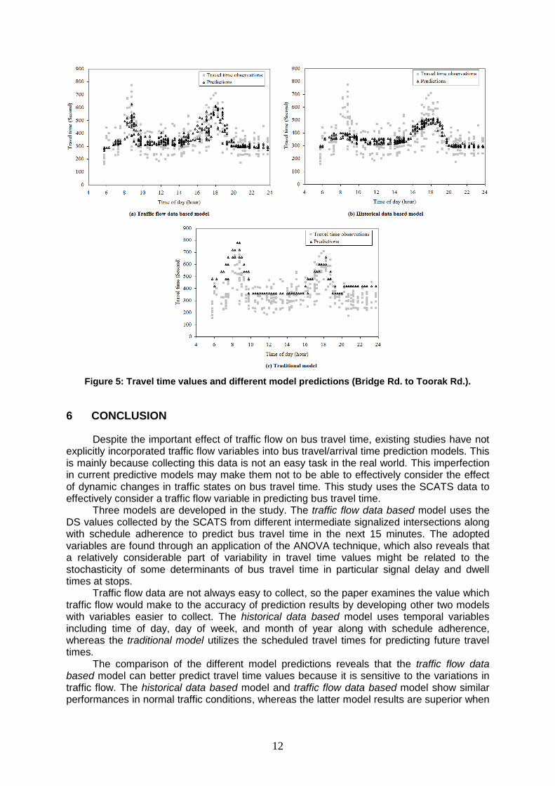
To obtain further insights into different model performances, Figure 4 and 5 depict the

distribution of observed travel times along with different model predictions for two sections over the day. As seen, the models with DS values can relatively present peak travel times,

11

whereas the models with temporal variables are sometimes not able to explain these peaks (e.g. morning peak in Figure 5).

The superiority of the traffic flow data based becomes dominant when there is an abnormal surge in traffic flow. In Figure 4(a), there are two points that are located away from other data points (one around mid-day, and the other one around 7:00pm). These two are fairly well located on their corresponding observed travel times. The inspection of traffic flow data revealed that the high observed travel times are due to high traffic volume, which the model could predict effectively.

As an operational policy, scheduled travel times are normally higher than actual travel times (e.g. morning peak in Figure 5(c)). This helps buses arrive on time relative to scheduled arrival times. However, they sometimes do not follow the overall travel time pattern over the day. For example, in Figure 4(c), while morning and evening peaks are observed in the travel time distribution, the scheduled travel times are constant over the day. This suggests possible improvements in timetable development.

The interesting conclusion drawn from this figure is that the DS variable only captures a part of day-to-day travel time variability at each time. For example, in Figure 4, at 12:00pm, travel time observations range from 250 to 550 seconds. When DS values are used to predict travel time (Figure 4(a)), the prediction values vary from about 300 to 400 seconds. The rest of the observed variation could be attributable to other factors such as variations in passenger demand, and variations in signal delay experienced by different buses. This conclusion is consistent with the results of Table 2.

Figure 4: Travel time values and different model predictions (Johnston St. to Bridge Rd.).

12

Figure 5: Travel time values and different model predictions (Bridge Rd. to Toorak Rd.).

6 CONCLUSION

Despite the important effect of traffic flow on bus travel time, existing studies have not explicitly incorporated traffic flow variables into bus travel/arrival time prediction models. This is mainly because collecting this data is not an easy task in the real world. This imperfection in current predictive models may make them not to be able to effectively consider the effect of dynamic changes in traffic states on bus travel time. This study uses the SCATS data to effectively consider a traffic flow variable in predicting bus travel time.

Three models are developed in the study. The traffic flow data based model uses the DS values collected by the SCATS from different intermediate signalized intersections along with schedule adherence to predict bus travel time in the next 15 minutes. The adopted variables are found through an application of the ANOVA technique, which also reveals that a relatively considerable part of variability in travel time values might be related to the stochasticity of some determinants of bus travel time in particular signal delay and dwell times at stops.

Traffic flow data are not always easy to collect, so the paper examines the value which traffic flow would make to the accuracy of prediction results by developing other two models with variables easier to collect. The historical data based model uses temporal variables including time of day, day of week, and month of year along with schedule adherence, whereas the traditional model utilizes the scheduled travel times for predicting future travel times.

The comparison of the different model predictions reveals that the traffic flow data based model can better predict travel time values because it is sensitive to the variations in traffic flow. The historical data based model and traffic flow data based model show similar performances in normal traffic conditions, whereas the latter model results are superior when

13

there is an abnormal surge in traffic flow. In a comparative sense, the traditional model shows the worst performance since it is not able to capture the variations in travel times.

The traffic flow data based model developed in this study can be regarded as a promising means for the use in advanced traveller information systems where collecting traffic flow is feasible. However, where collecting this data is not an easy task, the historical data based models can be used as a fairly „cheap‟ proxy to predict future travel times.

Among many factors affecting bus travel time, this study uses traffic flow data and schedule adherence to predict bus travel time. The inclusion of other variables such as passenger demand to predict bus travel time might improve the accuracy of the results. This is a promising direction for future studies.

7 Acknowledgement

The Ventura Bus Company, VicRoads, and Bureau of Meteorology are appreciated for supplying the GPS data, SCATS data and weather data respectively.

8 REFERENCES

Abdelfattah A. M. and Khan A. M., 1998, “Models for predicting bus delays”, Transportation Research Record, No. 1623, 8-15.

Bishop, C.M., 1995, “Neural networks for pattern recognition”, Clarendon Press, Oxford. Ceder, A., 2007, “Public transit planning and operation, theory, modelling and practice”,

Elsevier, Oxford, UK. Chien S. I., Ding Y. & Wei C., 2002, “Dynamic bus arrival prediction with artificial neural

networks”, Journal of Transportation Engineering, Vol. 128, No. 5, p.p. 429-438. Chen M., Liu X., Xia J. and Chien S. I., 2004, “A dynamic bus arrival time prediction model

based on APC data”, Computer Aided Civil and Infrastructure Engineering, Vol. 19, p.p. 364-376.

Chen M., Liu X., and Xia J., 2005, “Dynamic prediction method with schedule recovery impact for bus arrival time”, Transportation Research Record, 1923, pp. 208 – 217.

Chen M., Yaw J., Chien S.I., and Liu X., 2007, “Using automatic passenger counter data in bus arrival time prediction”, Journal of Advanced Transportation, Vol. 41, No. 3, pp. 267-283.

Dailey D. J., Maclean S. D., Cathey F. W. and Wall Z. R., 2001, “Transit vehicle arrival prediction; algorithm and large-scale implementation”, Transportation Research Record, No. 1771, p.p. 46-51.

Fu L., and Yang X., 2002, “Design and implementation of bus holding control strategies with real time information”, Transportation Research Record, No. 1791, p.p. 6-12.

Fu L., Lio Q., and Calamai P., 2003, “Real-time optimization model for dynamic scheduling of transit operations”, Transportation Research Record, No. 1857, p.p. 48-55.

Hagan M. T., Demuth H. B. and Beale M., 1995, “Neural Network Design”, PWS, Boston. Hastie, T., Tibshirani, R. and Friedman, J., 2001, “The elements of statistical learning, data

mining, inference, and prediction”, Springer-Verlag, New York. Hofman M. & Mahony M., 2005, “The impact of adverse weather conditions on urban bus

performance measures”, Proceedings of the 8th international IEEE conference on intelligent transportation systems, Vienna, Austria.

Jain, B.A. and Nag, B.N., 1997, “A performance evaluation of neural network decision models”, Journal of Management Information Systems, Vol. 14, pp. 201-216.

Jeong R. and Rilett L. R., 2004, “Bus arrival time prediction using artificial neural network model”, IEEE Intelligent Transportation System Conference, Washington, USA.

Kalman R. E., 1960, “A new approach to linear filtering and prediction problems”, Transactions of the ASME-Journal of Basic Engineering, Vol 82D, p.p. 35-45.

14

Kalaputapu R. and Demetsky M. J., 1995, “Modelling schedule deviations of buses using automatic vehicle location data and artificial neural networks”, Transportation Research Record, 1497, pp. 44 – 52.

Lin W.H. and Zeng J., 1999, “Experimental study of real-time bus arrival time prediction with GPS data, Transportation Research Record, No. 1666, p.p. 101-109.

Lin W.H., and Bertini R.L., 2004, Modelling schedule recovery processes in transit operations for bus arrival time prediction”, Journal of Advanced Transportation, Vol. 38, No. 3, pp. 347-365.

Mazloumi E., Currie G., and Ross G., 2008, “Causes of Travel Time Unreliability: a Melbourne Case Study", 31st Australian Transport Research Forum (ATRF), Gold Coast, Australia.

Mishalani R.G., McCord M.R., and Forman S., 2008, “Schedule-based and autoregressive bus running time modelling in the presence of driver-bus heterogeneity”, Lecture Notes in Economics and Mathematical Systems, Springer Series, pp. 301-317.

Osuna E.E., and Newell G.F., 1972, “Control strategies for an idealized public transportation system”, Transportation Science, Vol. 6, No. 1, pp. 52-71.

Palacharla, P.V. and Nelson, P.C., 1999, “Application of fuzzy logic and neural networks for dynamic travel time estimation”, International Transactions in Operational Research, Vol. 6, 1, pp. 145-160.

Patnaik J., Chien S. and Bladikas A., 2004, “Estimation of bus arrival times using APC data”, Journal of Public Transportation, Vol. 7, No. 1, p.p. 1-20.

Park T., Lee S., and Moon Y.J., 2004, “Real time estimation of bus arrival time under mobile environment”, Proceedings of International Conference on Computational Science and its Applications, pp. 1088–1096.

Shalaby A. & Farhan A., 2004, “Prediction Model of Bus Arrival and Departure Times Using AVL and APC Data”, Journal of Public Transportation, Vol. 7, No. 1.

Sun D., Luo H., Fu L., Liu W., Liao X., and Zhao M., 2007, “Predicting bus arrival time on the basis of global positioning system data”, Transportation Research Record, No. 2034, p.p. 62-72.