Embed Size (px)
Citation preview

Using satellite tagging and molecular techniques to improve the ecologically
sustainable fisheries management of shortfin makos (Isurus oxyrinchus) in the
Australasian region
Tactical Research Fund
Rogers, P.Ja., Corriganb, S. and Lowtherc. A.
July 2015
FRDC Project No. 2011/077
aSARDI Aquatic Sciences, West Beach, South Australia.
bHollings Marine Laboratory, 331 Fort Johnson, Charleston, USA.
cNorwegian Polar Institute, Hjalmar Johansensgata, Tromsø 9296, Norway
ii
© 2015 Fisheries Research and Development Corporation and South Australian Research and Development Institute. All rights reserved. ISBN: 978-1-921563-81-2
Using satellite tagging and molecular techniques to improve the ecologically sustainable fisheries management of shortfin makos (Isurus oxyrinchus) in the Australasian region. Tactical Research Fund.
2011/077
2015
Ownership of Intellectual property rights Unless otherwise noted, copyright (and any other intellectual property rights, if any) in this publication is owned by the Fisheries Research and Development Corporation and the South Australian Research and Development Institute. This work is copyright. Apart from any use as permitted under the Copyright Act 1968 (Cth), no part may be reproduced by any process, electronic or otherwise, without the specific written permission of the copyright owner. Neither may information be stored electronically in any form whatsoever without such permission.
This publication (and any information sourced from it) should be attributed to Rogers, P. J., Corrigan, S., and Lowther, A. South Australian Research and Development Institute (Aquatic Sciences) 2015, Using satellite tagging and molecular techniques to improve the ecologically sustainable fisheries management of shortfin makos (Isurus oxyrinchus) in the Australasian region. Tactical Research Fund. Adelaide, July.
Creative Commons licence All material in this publication is licensed under a Creative Commons Attribution 3.0 Australia Licence, save for content supplied by third parties, logos and the Commonwealth Coat of Arms.
Creative Commons Attribution 3.0 Australia Licence is a standard form licence agreement that allows you to copy, distribute, transmit and adapt this publication provided you attribute the work. A summary of the licence terms is available from creativecommons.org/licenses/by/3.0/au/deed.en. The full licence terms are available from creativecommons.org/licenses/by/3.0/au/legalcode.
Inquiries regarding the licence and any use of this document should be sent to: [email protected].
Disclaimer The authors warrant that they have taken all reasonable care in producing this report. The report has been through the SARDI internal review process, and has been formally approved for release by the Research Chief, Aquatic Sciences. Although all reasonable efforts have been made to ensure quality, SARDI does not warrant that the information in this report is free from errors or omissions. SARDI does not accept any liability for the contents of this report or for any consequences arising from its use or any reliance placed upon it. Material presented in these Administrative Reports may later be published in formal peer-reviewed scientific literature.
The information, opinions and advice contained in this document may not relate, or be relevant, to a reader’s particular circumstances. Opinions expressed by the authors are the individual opinions expressed by those persons and are not necessarily those of the publisher, research provider or the FRDC.
The Fisheries Research and Development Corporation plans, invests in and manages fisheries research and development throughout Australia. It is a statutory authority within the portfolio of the federal Minister for Agriculture, Fisheries and Forestry, jointly funded by the Australian Government and the fishing industry.
Researcher Contact Details FRDC Contact Details
Name:
Address:
Fax:
Phone:
Email:
SARDI Aquatic Sciences
2 Hamra Avenue
West Beach
08 8207 5481
0882075344
Address:
Phone:
Fax:
Email: Web:
25 Geils Court
Deakin ACT 2600
02 6285 0400
02 6285 0499
www.frdc.com.au
In submitting this report, the researcher has agreed to FRDC publishing this material in its edited form.

iii
Contents
ACKNOWLEDGMENTS ............................................................................................................................................ VI
ABBREVIATIONS ................................................................................................................................................... VII
EXECUTIVE SUMMARY ............................................................................................................................................ 1
INTRODUCTION ...................................................................................................................................................... 4
BACKGROUND ................................................................................................................................................................ 4 NEED ............................................................................................................................................................................ 6
OBJECTIVES ............................................................................................................................................................ 8
METHODOLOGY ...................................................................................................................................................... 9
RESULTS ............................................................................................................................................................... 23
DISCUSSION .......................................................................................................................................................... 55
CONCLUSIONS ...................................................................................................................................................... 66
IMPLICATIONS ...................................................................................................................................................... 68
RECOMMENDATIONS ........................................................................................................................................... 68
EXTENSION AND ADOPTION ................................................................................................................................. 70
REFERENCES ......................................................................................................................................................... 71
APPENDICES ......................................................................................................................................................... 81

iv
Tables
Table 1. Tag deployment statistics for satellite tracked shortfin makos between 2008 and 2013 .............. 13 Table 2. Details of mean bearing of the track per individual from the tagging location to each CRAWL
filtered position, mean swim speed, mean rate of movement distance travelled and distal displacement distance. ........................................................................................................................ 28
Table 3. Genetic diversity at mitochondrial DNA and nuclear microsatellite markers ................................. 38 Table 4. Pairwise measures of population differentiation based on mitochondrial DNA. ............................ 42 Table 5. Pairwise measures of population differentiation based on nuclear microsatellite data ................. 45 Table 6. Comparisons of pairwise measures of population differentiation for females and males based on
ΦST values for mitochondrial DNA (a) and GST’’ values for nuclear microsatellite
data……………………………………………………………………………………………………………..550
Table 7. F-statistics, relatedness, mean assignment and variance assignment for each sex .................... 51 Table 8. Tests of spatial autocorrelation and among sex correlogram heterogeneity ................................ 52 Table 9. Estimates of effective population size and associated upper and lower bounds of the 95%
confidence interval ............................................................................................................................... 54
Figures
Figure 1. Tagging locations of shortfin makos in Australia and New Zealand .............................................. 9 Figure 2. Locations, bathymetric and oceanographic features mentioned in the text of the report ............ 11 Figure 3. Cradle used to handle shortfin makos during deployment of satellite tags. ................................ 12 Figure 4. Regions and locations where tissue samples of shortfin makos were collected for genetic
analyses in the Southern and Northern Hemispheres. Locations sampled within regions are represented by the yellow square symbols. Regions include the Northern Atlantic, South Africa, Northern Indian, Western Australia, Indo Pacific, southern and eastern Australia and New Zealand. Western and southern Australia were grouped to comprise southwestern Australasia and the Indo-Pacific and eastern Australia were grouped to comprise eastern Australia for some analyses. ......... 16
Figure 5. Map showing tagging and recapture locations for shortfin makos............................................... 24 Figure 6. A. Wind-rose percentage frequency plots showing bearing of movement of shortfin mako from
their tagging location based on conventional tag-recapture data. B. Movement bearings for sharks tagged in NSW. C. Movement bearings for sharks tagged off Victoria ............................................... 25
Figure 7. CRAWL model fits to ARGOS data showed the spatial range occupied by shortfin makos, M1 and M2 in the GAB and Indian Ocean ................................................................................................. 29
Figure 8. CRAWL model fits to ARGOS data showing the spatial scale occupied by shortfin makos, M3 and M4 in the GAB, Bonney Upwelling Region, Subtropical Front, Indian Ocean and Bass Strait ..... 30
Figure 9. CRAWL model fits to ARGOS data showing the spatial scale occupied by shortfin makos, M5 and M6 in the GAB, Bonney Upwelling Region, and Bass Strait ......................................................... 31
Figure 10. CRAWL model fits to ARGOS data showing the spatial scale occupied by shortfin makos, M7 and M8 in the GAB, Bonney Upwelling Region, Subtropical Front, and Indian Ocean ........................ 32
Figure 11. CRAWL model fits to ARGOS data showing the spatial scale occupied by shortfin makos, M9 and M10 in the GAB, Bonney Upwelling Region, Subtropical Front, Tasman Sea, Coral Sea, SW Pacific and Indian Ocean ..................................................................................................................... 33
Figure 12. CRAWL model fits to ARGOS data showing the spatial scale occupied by shortfin makos, M11 and M12 in the Bonney Upwelling Region, Tasman Sea, Coral Sea, SW Pacific, New Zealand shelf waters and New Caledonia .................................................................................................................. 34
Figure 13. CRAWL model fit to ARGOS data showing the spatial scale occupied by shortfin mako M13 from the Bonney Upwelling Region across the GAB and during a trans-Indian Ocean migration ....... 35
Figure 14. CRAWL model fit to ARGOS data showing the spatial scale occupied by all shortfin makos M1–13 combined between 2008 and 2014. ................................................................................................ 36
Figure 15. Median joining network of 10 equally parsimonious trees ......................................................... 39 Figure 16. Statistical power of microsatellite data to detect various levels of true population differentiation
(FST) .................................................................................................................................................... 44 Figure 17. Plot of the estimated membership coefficients for each individual in each of two genetic clusters
............................................................................................................................................................. 46

v
Figure 18. Distribution of the randomized test statistics for detecting sex biased dispersal and frequency distribution of assignment indices for males and females. Assignment Indices were calculated and used to assess sex differences in assignment. ................................................................................... 48
Figure 19. Correlogram plots of the spatial autocorrelation coefficient, r as a function of geographical distance for males (in blue) and females (in red). Upper and lower bounds for the 95% confidence interval for the null hypothesis of no spatial structure (r = 0) based on 10, 000 random permutations of the data among distance classes are depicted as black dotted lines. 95% confidence intervals about r were determined using 10, 000 bootstrap replicates. Geographic distances presented are the maximum distance of each class......................................................................................................... 49
Figure. 20. Conceptual connectivity plots showing linkages determined from the four different data-sets in the Australasian and central Indo Pacific and South Africa, and the two ‘out-groups’, Northern Indian Ocean (Oman), and the North Atlantic (Portugal)................................................................................ 67

vi
Acknowledgments
This study was supported by funding provided by the Fisheries Research and Development
Corporation Tactical Research Fund (Shark Futures). Additional support was provided by Nature
Foundation SA Inc., Department for Environment and Natural Resources (DEWNR), Australian
Geographic Society, Victorian DEPI Recreational Fishing Trust, SARDI Aquatic Sciences, and
Flinders University. Procedures were undertaken under SARDI/PIRSA Ministerial exemptions
(Section 115; 9902094, and S59; 9902064), DEWNR Permit U25570, Environment Australia,
EPBC Act 1999 Permit E20120068 and Flinders University’s Animal Welfare Committee
approval (Project 309). Drs Simon Goldsworthy and Bradley Page assisted with funding support
for the tag deployments in 2008/09 and the ARGOS satellite network coverage. Conventional
game fish tagging data used in this report were provided by the NSW DPI Game Fish Tagging
Program funded by the NSW recreational Fishing Saltwater Trust as per the terms of the data
licence agreement between SARDI and NSW DPI (22 January 2014). We thank Phil Bolton and
Adam Welfare from NSW DPI for their assistance with our queries regarding the conventional
tagging data. Flinders University provided use of laboratory facilities to analyse tissue samples
during a related preliminary project funded by Seaworld. We thank the International participants
and Barry Bruce, the primary investigator of the FRDC funded workshop, Shark futures - a
synthesis of available data on mako and porbeagle sharks in Australasian waters: Current
status and future directions for constructive input and support of this project. Drs Andrew Oxley,
Nicole Patten and an FRDC assigned reviewer provided valuable comments and suggestions to
assist the improvement of the final version of this report. We also thank the following people for
their invaluable assistance during satellite tag deployments: John Collinson, Anton Blass, Callan
Henley, Shane Gill (FV Rahi Aroha), Dennis and Kerry Heineke, Adam Todd (FV Shaka-Zura),
Paul Irvine, Steve Toranto, Phil Stroker, Clinton Adlington (FV Home Strait), Shane Sanders and
Brodie Carter (FV Baitwaster), Charlie Huveneers, Matt Heard, Mick Drew, Crystal Beckmann
(SARDI), Slavko Kolega, Chris Meletti (Sekol, MV Lucky-S), Mark Lewis and Bruce Barker
(CSIRO). Four sharks were tagged with support from an aligned project funded by the Victorian
Department of Primary Industries Recreational Fishing Licence Trust Account Large Grants
Program. Tissue samples for genetic analyses were provided by: Malcolm Francis, Clinton
Duffy, Nuno Queiroz, Gonzalo Mucientes, Geremy Cliff, William White, Charlie Huveneers,
Lindsay Marshall, Matias Braccini, Rory McAuley, Julian Peperrell, Rima Jabado, Alan Foulis,
Gavin Naylor, John Collinson, Paul Irvine, Steve Toranto, Shane Sanders, Brodie Carter, Adam
Todd, Dennis and Kerry Heineke, Ashley and Neville Dance, and Greg Barea. Luciano
Beheregaray and Gavin Naylor provided funding and infrastructure support for the genetic
analyses. Dovi Kacev and John Hyde (NOAA/NMFS) developed the microsatellite markers and
we thank them for sharing primer sequences.

vii
Abbreviations
Australian Fisheries Management Authority (AFMA)
Commission for the Conservation of Southern Bluefin Tuna (CCSBT)
Commonwealth Scientific and Industrial Research Organisation (CSIRO)
Convention on International Trade in Endangered Species of Wild Flora and Fauna (CITES)
Convention on Migratory Species (CMS)
Department for Environment and Natural Resources (DEWNR)
Exclusive Economic Zone (EEZ)
Ecologically Related Species Working Group (ERSWG)
Environmental Protection Biodiversity and Conservation Act 1999 (EPBC Act 1999)
Game Fishing Association of Australia (GFAA)
Great Australian Bight (GAB)
Fisheries Research and Development Corporation (FRDC)
Highly Migratory Species (HMS)
International Game Fishing Association (IGFA)
International Union of Conservation of Nature (IUCN)
Indian Ocean Tuna Commission (IOTC)
International Commission for the Conservation of Atlantic Tunas (ICCAT)
National Oceanic and Atmospheric Administration (NOAA)
Regional Fisheries Management Organisation (RFMO)
South Australian Research and Development Institute (SARDI)
Secretariat of Pacific Community (SPC)
Species Survival Commission (SSC)

viii
Sub-Tropical Front (STF)
Threatened Endangered and Protected Species (TEPS)
Western Central Pacific Fisheries Commission (WCPFC)
1
Executive Summary
This study used a multi-disciplinary approach to investigate the patterns of population
structure, spatial connectivity, and contemporary effective population size of the
shortfin mako (Isurus oxyrinchus). It represents the first comprehensive study of the
connectivity of this Highly Migratory Species (HMS) species in the Southern
Hemisphere.
Listing of the shortfin mako under the Environmental Protection Biodiversity and
Conservation Act (EPBC Act, 1999) in 2010 was debated by recreational/game
fishers. This was followed by an amendment to allow that sector to continue to target
shortfin makos. Points of contention included a perception that there was: 1) limited
information available to assess links between shortfin mako populations in Australian
waters and those in the Northern Hemisphere, and 2) limited information on the
movement and mixing of shortfin makos that support Australian fisheries.
The Fisheries Research and Development Corporation funded an Australasian Mako
Shark Workshop in 2012. Information on the population structure of the shortfin
mako was identified as a research gap and this provided part of the impetus for this
project.
The shortfin mako represents a significant recreational and game fish target and
bycatch species of pelagic fisheries that target tuna and billfish.
Methodologies used included spatial analyses of long-term satellite telemetry and
conventional tagging data from southern and eastern Australia, and analyses of DNA
data from the mitochondrial (DNA sequence) and nuclear (microsatellite) genomes
from samples collected between New Zealand, Australasia and Indo-Pacific, western
Indian Ocean and North Atlantic Ocean.
We used ARGOS tracking data and a (C)orrelated (RA)ndom (W)alk (L)ibrary
(CRAWL) model and state-space framework to establish spatial parameters,
including mean rate of movement per day (ROM), minimum cumulative distance
travelled, and distal displacement distances for each tagged individual.
A total of 7,328 shortfin makos were conventionally tagged and released in
Australian waters by recreational and game fishing anglers (NSW DPI Game Fish
Tagging Program) between 1973 and 2014. Of these, 158 (2.2% of 7,328) were
recaptured between 1977 and 2013. Displacement distances from the tagging sites
ranged between 0 and 5,940 km (mean = 532 ± 62.04 km).

2
The maximal extents of migrations by satellite tagged shortfin makos were north to -
12.13°S, south to -46.00°S, east to 174.69°E and west to 49° E. The spatial scales of
movements over periods up to 1.8 years ranged between 8,776–24,213 linear km in
the Great Australian Bight, Indian Ocean and Coral Sea, and up to 10,838 km in a ~1
year period between the eastern Bass Strait, New Zealand, and New Caledonia
regions.
Analyses of mitochondrial DNA suggested there was limited population structure
within Australian management jurisdictions, although southern Australia and New
Zealand may be connected via patterns of step-wise mitochondrial gene flow.
Cross-equatorial mitochondrial gene flow was limited. Both Northern Hemisphere
sampling sites showed significant differentiation from those in the Southern
Hemisphere. There was some evidence of reduced mitochondrial gene flow across
the Indian Ocean between Australasia and South Africa, however this requires
further investigation.
In contrast to the results based on mitochondrial DNA, microsatellite data indicated
high connectivity between all sampling locations within Australian management
jurisdictions, and with neighbouring sampling sites in South Africa and the Northern
Hemisphere. However, given the results from the mitochondrial DNA, we caution
against interpreting this to mean that shortfin mako be managed as a single
panmictic stock since the migration rate necessary to eradicate a signal of stock
structure is less than would be required to replenish overharvested populations by
migration.
Contrasting levels of mitochondrial and microsatellite structure at the ocean basin
level may indicate that sex-biased dispersal is occurring at this geographic scale.
There was a trend toward male-biased dispersal evident in analyses based on
smaller spatial scales, however this was not statistically supported. Several caveats
to the statistical power of this analysis are discussed. It was recommended that sex-
biased dispersal is reassessed based on a larger sample size of both tracking and
genetic data derived from mature individuals of known sex.
Estimates of contemporary effective population size mostly ranged between the
orders of 100s to 1,000s. Estimated effective population size for the Australasian
region (Indo-Pacific, eastern, southern, Western Australia and New Zealand) was
2,550.6 (95% CI = 831 – ∞). Difficulties associated with estimating effective
population size in large populations, including some unavoidable violations of
3
analysis assumptions, are discussed.
In summary, based on the 36 year conventional tagging data-set, a 7-year satellite
tracking dataset, and microsatellite and mitochondrial DNA analyses from 365
samples collected in six key regions, the most appropriate ecological scale at which
to manage the population fished in Australian State and Commonwealth waters are
the boundaries of the Australian and Central Indo Pacific Region (New Zealand –
south west Pacific – Australasian/Indo Pacific Region). This will need to be refined as
further satellite tracking data are collected and as we collect genetic data from the
north and south east Pacific Ocean, and southern Indian Ocean.
Future research should seek to improve satellite tracking and genetic datasets for
adult shortfin makos, identify regions in the Australasian and Central Indo-Pacific
Region used for nursery, pupping and parturition, and to improve information on the
size of breeding populations.
Keywords: Shortfin mako, Isurus oxyrinchus, stock structure, connectivity, movement, migration.
4
Introduction
Background
There is a growing awareness of the important functional roles of top predators, including
pelagic sharks (Dulvy et al. 2008; Ferretti et al. 2010), in maintaining marine ecosystem
health. Consequently, there is an increasing expectation that fisheries impacts be managed
appropriately. Highly migratory species (HMS) of pelagic sharks represent an ecologically,
commercially and socially important, but challenging group to manage due to their cryptic
nature, ongoing uncertainties regarding their distributions and abundance, and high mobility
with a propensity to move across multi-jurisdictional management boundaries (Heithaus et al.
2008; Baum and Worm 2009). Incorporating information regarding the distributions,
movement patterns, genetic structure and sizes of pelagic shark populations is therefore
crucial to the development of effective management strategies.
Australia is a major fishing nation in the Southern Hemisphere, contributing substantially to
pelagic shark target catch and bycatch in this region. Australia is a signatory to multiple
international treaties and assessment entities. These include the Convention on Migratory
Species (CMS), the Convention on International Trade in Endangered Species of Wild Flora
and Fauna (CITES) and the International Union of the Conservation of Nature (IUCN)
Species Survival Commission (SSC); all of which call for the integration of modern
investigations into the ecological and demographic attributes of HMS, to guide conservation
and management options. Nevertheless these areas represent existing knowledge gaps for
the majority of pelagic shark species with ranges that extend into this region.
The shortfin mako (Family: Lamnidae, Isurus oxyrinchus) is a globally iconic, oceanic pelagic
shark species with an extensive temperate and tropical distribution (Compagno et al. 2005),
ranging across multiple international and high seas management jurisdictions. It is thus an
excellent example of a species that presents substantial challenges in terms of sustainable
fisheries and bycatch management in high seas of Australasia and the Indo-Pacific. Bycatch
in commercial pelagic long-line fisheries targeting tunas, broadbill swordfish and billfish
represent a key source of mortality of shortfin makos in Australian Commonwealth and
neighbouring jurisdictions (Stevens 1992; Bruce 2014). Between 1998 and 2011, there were
~852 t (trunk wt) of shortfin makos recorded in Australian Commonwealth managed
fisheries, with the majority (757 and ~17.7 t) taken in the Eastern and Western Tuna and
Billfish Fisheries (ETBF and WTBF; Bruce 2014). In the early 2000s the Australian Fisheries

5
Management Authority (AFMA) banned at-sea finning of sharks, which has had important
implications for the sustainable management of Australasian stocks. Landing and retaining
of live shortfin makos is currently not permitted in State and Commonwealth fisheries,
however dead individuals can still be retained under trip limits of 20 shark for all species
combined. These sharks can be finned legally once they have been landed on shore.
Previous genetic studies of the shortfin mako showed significant mitochondrial structuring
between the Pacific and Atlantic Ocean basins, as well as cross-equatorial sub structure
within ocean basins, and between the southeast and southwest Pacific Ocean (Heist et al.
1996; Schrey and Heist 2003). However, the null hypothesis of a single globally panmictic
genetic stock could not be rejected based on data from nuclear microsatellite markers
(Schrey and Heist 2003). Together these patterns indicate that gene flow at a global scale is
male mediated in shortfin mako, while females exhibit greater philopatry to ocean basins
(Schrey and Heist 2003). Philopatry in coastal and offshore oceanic areas has also been
suggested to occur in white sharks (Carcharodon carcharias) that migrate between these
areas in the Pacific Ocean (Jorgensen et al. 2010). Tagging data for shortfin makos also
indicate differentiation between Northern and Southern Hemisphere populations. Following
more than 21,000 standard and satellite tag deployments globally, only one individual has
been reported to cross the equator (Holts 1988; Holts and Bedford 1993; Francis et al. 2001;
Klimley et al. 2002; Kohler et al. 2002; Sepulveda et al. 2004; Loefer et al. 2005; Holdsworth
and Saul 2010; Stevens et al. 2010; Wraith and Kohin 2010; Abascal et al. 2011; Block et al.
2011). Additionally, satellite tracking studies have shown that while shortfin makos exhibit
both broad-scale movements and periods of fidelity in the Southern and Indian Oceans
(Rogers et al. 2015), they also exhibit similar patterns in the northwest Atlantic Ocean, the
southeast, central and northeast Pacific Ocean (Vetter et al. 2008; Abascal et al. 2011; Block
et al. 2011; Loefer et al. 2005; Musyl et al. 2011), and the southwest Pacific Ocean off
eastern Australia (Stevens et al. 2010).
High mobility does not imply high gene flow (Palumbi 2003). Animals may move for reasons
that are unrelated to reproductive activity [for example, in response to prey distribution or
habitat preferences], which doesn’t translate into genetic connectivity between regions. Other
factors, such as sex-biased dispersal, geographical and ecological barriers to movement,
recent evolutionary history or an historical demographic event may also promote genetic
structure in HMS (Avise 2004). Although studies to date have provided critical insights into
the movement ecology of shortfin mako, more information is needed to determine the
appropriate spatial scale at which to manage this species in Australasian waters.
Specifically, the extent of connectivity between locations within the Southern Hemisphere is

6
poorly understood, as this region has previously received only low geographic sampling
coverage. Tagged animals have mostly been tracked in the Northern Hemisphere while DNA
sampling has been conducted only at the ocean basin level. Developing sound management
strategies for shortfin makos in Australasian waters requires determining whether any
unrecognised local substructure exists throughout the region and between neighbouring
jurisdictions.
An understanding of movement ecology for management purposes therefore requires that
movement be directly quantified in order to identify critical habitats, but also that the genetic
consequences of movement are understood (i.e. gene flow), as these are intimately related
to population persistence (Nams 2006; Dingle and Drake 2007). Tracking methods are
useful for obtaining direct estimates of dispersal and fine-scale movement of individuals.
Molecular methods allow assessments of genetic connectivity over broader spatial scales.
We therefore employed the multi-disciplinary approach of combining satellite tracking,
conventional tagging, and DNA datasets to investigate the spatial scales of movements and
population structure of shortfin makos sampled around Australia and those in neighbouring
regions (e.g. Indian Ocean and New Zealand waters).
Genetic data may be used to estimate the contemporary effective population size (CNe). For
fisheries management purposes, CNe can be thought to approximate the recent average
number of breeding individuals that have contributed to the observed genetic diversity within
a population (Luikart et al. 2010; Hare et al. 2011). Reductions in population size can be
associated with loss of genetic diversity and adaptive variation, increased inbreeding and the
accumulation of deleterious alleles, all of which have negative consequences for long term
population survival and evolutionary potential (Frankham et al. 2010). Estimating CNe
therefore, indicates not only the breeding population size, but can also provide a measure of
population genetic health. Genetic monitoring and CNe estimation has featured heavily in
conservation plans for terrestrial organisms but has only been a focus in marine
conservation planning in recent years. To date, CNe has been estimated for few
elasmobranch species (Ahonen et al. 2009; Portnoy et al. 2009; Chapman et al. 2011;
Nance et al. 2011; Blower et al. 2012). There is scope for more widespread estimation of
CNe as an evaluation tool for marine populations, complementing existing stock assessment
methods (Luikart 1998; Hare et al. 2011).
Need
Concern for shortfin mako populations in the Northern Hemisphere led to the listing of this
species as ‘Critically Endangered’ in the Mediterranean and ‘Vulnerable’ in other regions,

7
including the North Atlantic by the International Union for Conservation of Nature Species
Survival Commission on 22 February 2007. Shortfin mako was subsequently CMS listed
(Appendix II: Migratory) which led to nomination under the Australian Commonwealth
Environment Protection Biodiversity and Conservation Act (EPBC Act, 1999). In November
2009, the Australian Commonwealth Government Department of the Environment released
information online stating that from 29 January 2010, shortfin mako, longfin mako (I.
paucus), and porbeagle (Lamna nasus) were to be listed under the EPBC Act, making it an
offence to kill, injure, take, trade, keep or move shortfin mako in Commonwealth waters.
EPBC Act provisions also afforded protection measures for each species in State (out to 3
nm), and Commonwealth waters.
The EBPC listing was debated and petitioned against by recreational, game and charter
fishers. Most of the conjecture was raised in Victoria, Tasmania and New South Wales,
where recreational fishers target shortfin makos. This led to an amendment to the EPBC Act
that allowed recreational fishers to continue to target shortfin makos. Points of contention
included that there was: 1) limited information available to assess connectivity between
Australian shortfin mako populations and those in the Northern Hemisphere, and 2) limited
information regarding the movements of the shortfin makos that support the Victorian
recreational fishery, and their connectivity with populations in other regions of Australia. In
early February 2012, the Australasian Mako Shark Workshop, which was run by CSIRO in
Hobart and funded by the Fisheries Research and Development Corporation (FRDC), aimed
to identify key research priorities for shortfin makos. Participants included scientists from the
CSIRO, Fisheries Departments of Tasmania, Victoria, New South Wales, Queensland, South
Australia and Western Australia, and overseas experts from New Zealand, USA, and
Secretariat of Pacific Community (SPC). Government officials from AFMA and the
Department of Environment also attended, as did representatives from the World Wide Fund
for Nature, Humane Society International and the game fishing sector (GFAA). AFMA
representatives indicated that information on the abundance of shortfin makos was a key
priority for management of tuna and billfish fisheries. This process highlighted that in
Australian jurisdictions, commercial fisheries catches of shortfin makos have predominantly
occurred in eastern Australian waters, with 1,257–3,288 (mean = 2,009) individual sharks
being landed per year, with 87% retained and 13% discarded (Bruce 2014). Collecting
further information about the genetic population structure of shortfin makos in the region was
also identified as a key research priority.

8
Objectives
This study aimed to assess population connectivity of shortfin makos within Australasian and
neighbouring waters by combining empirical satellite-tracking and conventional tagging data
with DNA data from mitochondrial and nuclear genomes. The resultant information will be
used to inform management strategies for shortfin makos in Australian and neighbouring
high seas jurisdictions, where this species ranges across multiple State, Commonwealth and
international boundaries. A multi-disciplinary approach to assessing connectivity in this
pelagic shark species is considered more powerful for detecting and defining management
boundaries when compared to single-discipline approaches because it allows consideration
of movements that may not be related to reproductive activity, but may reveal critical habitat,
while also indicating the extent of genetic connectivity between locations.
The specific aims of this study were:
1. To use new genetic data to assess the patterns of population genetic structure of
shortfin makos in the Australasian and neighbouring regions;
2. To compare the geographic scale of genetic connectivity with movement patterns
determined from conventional and satellite tagging;
3. To use the data to determine the contemporary effective population size of identified
spatially discrete stocks;
4. To integrate the genetic and movement data with that generated during a larger
global population structure study with special reference to elucidating the degree of
cross-equatorial dispersal.

9
Methodology
Conventional tag-recapture
Conventional tag-recapture data were collected for 158 shortfin makos (Isurus oxyrinchus)
by recreational, game and commercial fishers in State and Commonwealth managed waters
of South Australia, Victoria, New South Wales, Queensland, and Western Australia during
the New South Wales Department of Primary Industries (DPI) Game Fish Tagging Program.
This tagging program began in 1973 and provides recreational and game fishers with
independently numbered stainless steel head plastic identification tags and tag cards to
record capture and release information, including the method of capture, condition on
release, species identification, date and location of capture (lat-long), and an estimate of size
and weight. Conventional tagging data were returned by anglers and fishing clubs and stored
in the NSW DPI Game Fish Tagging Program database. Figure 1 shows tagging locations
for recaptured shortfin makos between 1973 and 2014. Appendix 1 provides summary
details of all tag-recapture events.
Figure 1. Tagging locations of recaptured shortfin makos in Australia and New Zealand between 1973 and 2014 (indicated by yellow symbols) (Bathymetry source: NOAA ETOPO1 Global relief bathymetry layer (Amante and Eakins 2009).

10
Capture and tagging techniques
Conventional tagging of sharks occurs via the following steps: a shark is hooked on game
fishing equipment and brought along-side the vessel by an angler; the leader is held while a
designated tagger uses a tag pole with a stainless steel applicator needle to apply the tag
into the musculature near the first dorsal fin; the shark is released by removing the hook(s)
using a purpose built de-hooking device, or the leader is cut as close to the shark’s
mouth/hook(s) as possible. Following a recapture, the fishers record the tag ID number,
species, date, location (lat-long), estimated or actual size (if landed and retained), and
physical condition upon release (if applicable).
Data analyses
The spatial scale of movement of each tagged shark was estimated by plotting the tag-
recapture locations over the NOAA ETOPO1 Global relief bathymetry layer (Amante and
Eakins 2009) using MapInfo Ver. 11.5 (Mapinfo Corporation, New York) geographical
information systems (GIS) software, removing erroneous locations (i.e. locations on land).
Minimum displacement distances (mean, standard error and 5–95th percentiles) travelled
between the tagging and recapture locations were measured along with the number of days
at liberty. We calculated the individual bearings (direction) between the tagging and
recapture locations. Percentage frequencies based on bearing estimates (40° bins) were
examined using wind-rose plots in OriginPro 9.1 software (OriginLab, Northampton, USA).
Satellite tagging
A total of 13 satellite tags were deployed in the Great Australian Bight (GAB), southeastern
South Australia, western and eastern Victoria between 2008 and 2013 (Fig. 2). Satellite tags
were deployed at locations in continental shelf and shelf slope waters of the GAB and the
south-east coast of South Australia in 2008 and 2009, and in shelf waters of southwestern
Victoria and Bass Strait in 2012 and 2013. Tag deployment sites, locations and bathymetric
and oceanographic features mentioned in this report are shown in Figure 2. In Bass Strait,
two tags were deployed at a single location. Deployment summary details, including shark
size, sex and tagging locations are provided in Table 1. Tags deployed included five different
dorsal fin mounted configurations, including Sirtrack™ KiwiSat 202, Sirtrack K2F161A,
Wildlife Computers™ (WC) Smart Position or Temperature (SPOT), and data collecting
11
Argos tags (SPLASH) and Mk10A. Sirtrack 202 tags and SPOTs were programmed to
transmit daily, whereas the SPLASH and Sirtrack K2F161A tags were duty-cycled to transmit
at a 2-day frequency to maximise battery life.
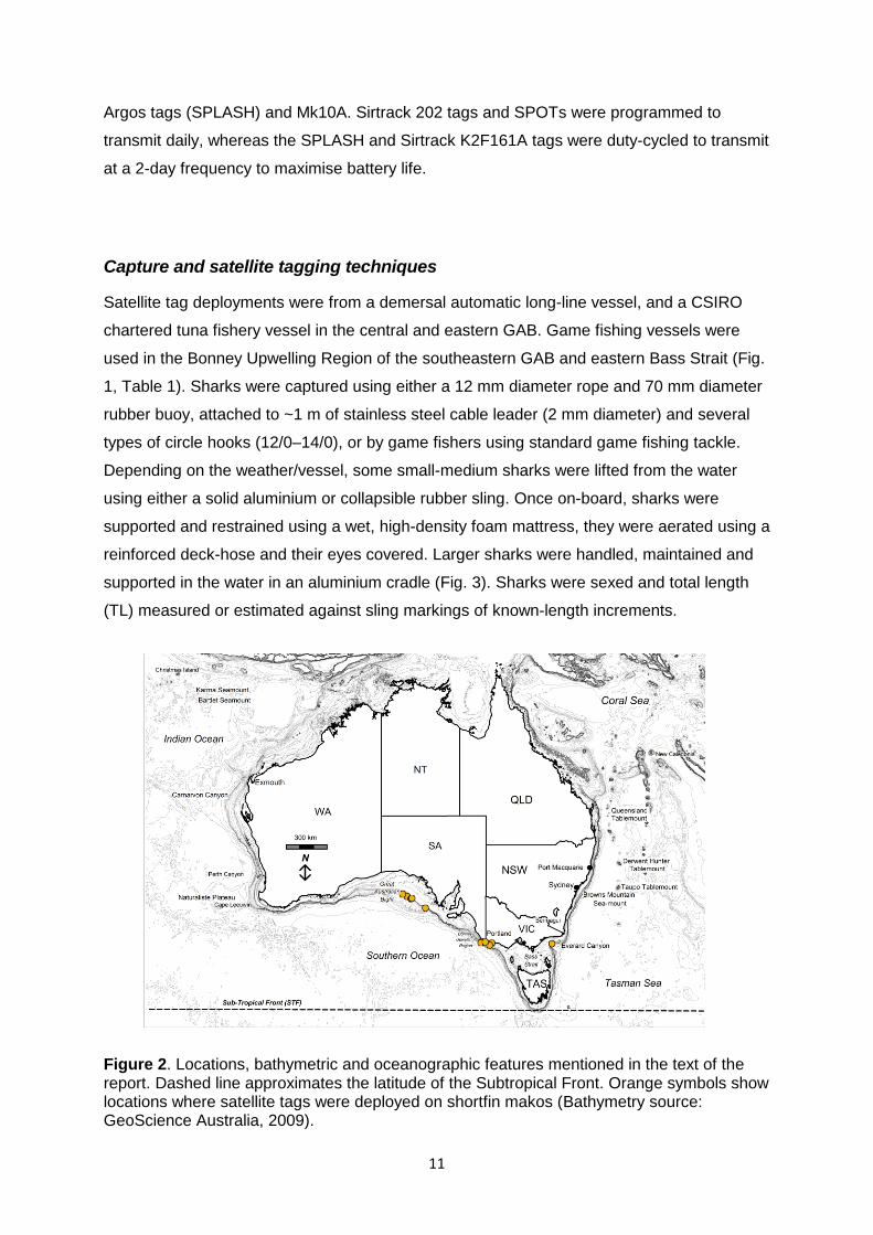
Capture and satellite tagging techniques
Satellite tag deployments were from a demersal automatic long-line vessel, and a CSIRO
chartered tuna fishery vessel in the central and eastern GAB. Game fishing vessels were
used in the Bonney Upwelling Region of the southeastern GAB and eastern Bass Strait (Fig.
1, Table 1). Sharks were captured using either a 12 mm diameter rope and 70 mm diameter
rubber buoy, attached to ~1 m of stainless steel cable leader (2 mm diameter) and several
types of circle hooks (12/0–14/0), or by game fishers using standard game fishing tackle.
Depending on the weather/vessel, some small-medium sharks were lifted from the water
using either a solid aluminium or collapsible rubber sling. Once on-board, sharks were
supported and restrained using a wet, high-density foam mattress, they were aerated using a
reinforced deck-hose and their eyes covered. Larger sharks were handled, maintained and
supported in the water in an aluminium cradle (Fig. 3). Sharks were sexed and total length
(TL) measured or estimated against sling markings of known-length increments.
Figure 2. Locations, bathymetric and oceanographic features mentioned in the text of the report. Dashed line approximates the latitude of the Subtropical Front. Orange symbols show locations where satellite tags were deployed on shortfin makos (Bathymetry source: GeoScience Australia, 2009).

12
Figure 3. Cradle used to handle shortfin makos during deployment of satellite tags.

13
Table 1. Tag deployment statistics for satellite tracked shortfin makos between 2008 and 2013. **denotes tag still reporting at the time of report preparation.
Shark #
ARGOS ID
Tag type and
manufacturer Location
Deployment
date Sex
TL
(cm)
Time at liberty
(days)
ARGOS
position
estimates
cls 3–B
M1 55947 Sirtrack 202 -34.15, 132.42 11-03-08 M 170 672 1589
M2 55951 WC SPLASH -33.96, 131.95 01-06-08 F 180 496 702
M3 52465 WC SPOT -33.75, 131.45 30-03-09 F 180 458 1255
M4 52471 WC SPOT -38.17, 140.55 09-05-09 M 215 262 803
M5 115559 WC Mk10A -38.50, 141.68 17-12-12 F 260 320 1671
M6 115562 WC Mk10A -38.49, 141.43 28-6-12 F 270 249 1372
M7 52466 WC SPLASH -34.18, 132.41 04-06-08 F 200 469 594
M8 52478 WC SPOT -35.07, 134.07 22-11-09 M 170 324 1279
M9 115561 WC Mk10A -38.28, 140.43 05-05-12 M 220 320 1522
M10 55952 WC SPLASH -34.13, 132.52 31-03-09 F 240 482 528
M11 115162** Sirtrack 161A -38.36, 148.57 10-7-13 F 180 311 383
M12 115159** Sirtrack 161A -38.36, 148.57 11-7-13 F 190 318 452
M13 52481 WC SPLASH -38.21, 140.94 07-05-09 M 170 551 1221

14
Sexual maturity was assessed rapidly based on physical characteristics and size at maturity
for each sex following Francis and Duffy (2005). Steps were taken to minimise handling time
and mitigate associated stress during the tagging procedure. Specifically, the stainless steel
tag bolts were pre-glued into each tag using Araldite™ epoxy; a modified Stanley™ bench-
clamp attached to a tag shape template was used to enable holes to be drilled in the dorsal
fin that accurately matched the spacing of the tag bolts. Satellite tags were attached to the
first dorsal fin of each shark using only two or 3.5 mm diameter stainless steel bolts, nylex
lock-nuts and washers. Lock-nuts were fastened using a cordless drill and deep socket and
the total length of each animal was estimated (± 10 cm) from increments marked on the
cradle. Prior to the release of each shark, bolt cutters were used to remove the hook or cut it
in half in a manner that would allow loss of the hook remnant from the jaw.
Data analyses
Satellite tags transmitted signals to the low polar orbiting environmental satellite network
receiver stations, which were forwarded to ARGOS centres in France and the USA (ARGOS,
2008). ARGOS position estimates were accessed using Telnet and Tera Term Pro software.
Position data were downloaded in seven location classes (cls) ranging from highest to lowest
between 3, 2, 1, 0, A, B and Z (no positions) with manufacturer predicted accuracies of 3 =
<250 m, 2 = 250–500 m, 1 = 500–1500 m and 0–B = >1500 m, Z = no position (www.argos-
system.org). ARGOS position estimation error has also been directly compared to GPS
positions and the 68th percentile errors were 3 = 0.49 km, 2 = 1.01 km, 1 = 1.2 km, 0 = 4.18
km, A = 6.19 km, and B = 10.28 km (Costa et al. 2010). Positions of all classes were
mapped using circular symbols in the GIS software package, MapInfo Ver. 11.5 (Mapinfo
Corporation, New York) on the NOAA ETOPO1 Global relief bathymetry layer (Amante and
Eakins 2009) and the Australian bathymetry and topography grid at 250 m resolution
(GeoScience Australia 2009). Raw ARGOS data were pre-processed to remove extreme
outliers, positions on land and those with unclassified error estimates (cls-Z). Filtering of
ARGOS data were undertaken by estimating locations using a Kalman filter under a
continuous-time state-space framework using the (C)orrelated (RA)andom (W)alk (L)ibrary
‘CRAWL’ package in R Ver. 2.15.2 (Johnson et al. 2008; R core team 2013). Locations were
interpolated along each filtered track to reduce sampling bias due to irregular transmission of
ARGOS location data. We calculated the mean and frequency of individual bearings from
the tagging locations to each CRAWL filtered position. To establish a set of spatial scale-
based movement parameters, we estimated mean rate of movement per day (ROM),
minimum cumulative distance travelled based on the individual CRAWL filtered tracks and
15
distal displacement distances for each individual (difference between tagging location and
most distant location). Statistical results were reported as mean ± standard error with 5th
and 95th percentiles, unless otherwise stated.
Population genetics
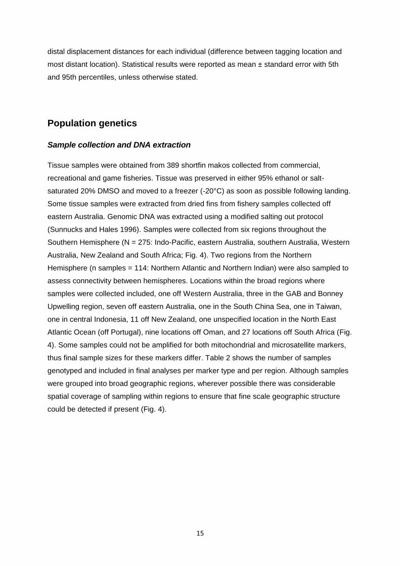
Sample collection and DNA extraction
Tissue samples were obtained from 389 shortfin makos collected from commercial,
recreational and game fisheries. Tissue was preserved in either 95% ethanol or salt-
saturated 20% DMSO and moved to a freezer (-20°C) as soon as possible following landing.
Some tissue samples were extracted from dried fins from fishery samples collected off
eastern Australia. Genomic DNA was extracted using a modified salting out protocol
(Sunnucks and Hales 1996). Samples were collected from six regions throughout the
Southern Hemisphere (N = 275: Indo-Pacific, eastern Australia, southern Australia, Western
Australia, New Zealand and South Africa; Fig. 4). Two regions from the Northern
Hemisphere (n samples = 114: Northern Atlantic and Northern Indian) were also sampled to
assess connectivity between hemispheres. Locations within the broad regions where
samples were collected included, one off Western Australia, three in the GAB and Bonney
Upwelling region, seven off eastern Australia, one in the South China Sea, one in Taiwan,
one in central Indonesia, 11 off New Zealand, one unspecified location in the North East
Atlantic Ocean (off Portugal), nine locations off Oman, and 27 locations off South Africa (Fig.
4). Some samples could not be amplified for both mitochondrial and microsatellite markers,
thus final sample sizes for these markers differ. Table 2 shows the number of samples
genotyped and included in final analyses per marker type and per region. Although samples
were grouped into broad geographic regions, wherever possible there was considerable
spatial coverage of sampling within regions to ensure that fine scale geographic structure
could be detected if present (Fig. 4).

16
Figure 4. Regions and locations where tissue samples of shortfin makos were collected for genetic analyses in the Southern and Northern Hemispheres. Locations sampled within regions are represented by the yellow square symbols. Regions include the Northern Atlantic, South Africa, Northern Indian, Western Australia, Indo Pacific, southern and eastern Australia and New Zealand. Western and southern Australia were grouped to comprise southwestern Australasia and the Indo-Pacific and eastern Australia were grouped to comprise eastern Australia for some analyses.

17
Genotyping
A total of 791 base pairs of the mitochondrial DNA control region was amplified by
Polymerase Chain Reaction (PCR) (Michaud et al. 2011). Purified DNA was bi-directionally
sequenced using BigDye® Terminator chemistry on an ABI 3730xl genetic analyzer (Applied
Biosystems®, Life Technologies, Grand Island USA) at Retrogen Inc. Custom DNA
Sequencing Facility (San Diego, USA).
Ten microsatellite loci were amplified using PCR primers described in Schrey and Heist
(2002) (Iox-12, Iox-30) and Kacev et al. (unpublished data) (Iox-B3, Iox-M1, Iox-M36, Iox-
M115, Iox-D123, Iox-M59, Iox-M110, Iox-M192). The forward primer of each pair was tailed
with an M13 tag that was incorporated with an M13 labelled fluorescent dye during PCR
cycling (Schuelke 2000). Reactions were conducted in 5 L volumes comprising 15–30 ng
template DNA, 3 mM MgCl2, 1× MangoTaq reaction buffer, 0.1 mM each dNTP, 0.1 pmol
M13 tailed forward primer, 0.3 pmol reverse primer, 0.1 pmol M13 fluorescently labeled
primer, 0.5 µg bovine serum albumin and 0.25 U MangoTaq™ DNA polymerase (Bioline,
Taunton USA). PCR cycling consisted of initial denaturation at 94°C followed by ‘touchdown’
cycling of 30 s denaturation at 94° C, 45 s annealing, and 1 min extension at 72° C.
Annealing temperature began at 65° C and decreased by 2° C at each touchdown,
stabilising at 57° C for 30 cycles. Products were separated on an ABI 3730xl genetic
analyzer (Applied Biosystems®, Life Technologies, Grand Island USA). Reference samples
for each locus were included in all PCR programs and during capillary separation of
fragments so as to ensure consistency in genotype calling. Any reactions that failed to
amplify initially, or that returned ambiguous genotypes, were re-amplified in order to minimise
both missing data and scoring error.
Mitochondrial DNA sequence data
DNA sequences were edited and aligned using Geneious® Pro v. 6.1.7 (Biomatters Ltd
Auckland, New Zealand. Available at http://www.geneious.com). Maximum-likelihood values
for different models of sequence evolution were obtained using jModelTest v. 0.1.1 (Posada
2008). According to the Corrected Akaike Information Criterion (Sugiura 1978), the Jukes
and Cantor model (Jukes and Cantor 1969), without among site rate variation or invariant
sites, was the most likely model of DNA substitution. Assuming this model, Arlequin v.
3.5.1.2 (Excoffier and Lischer 2010) was used to assess sequence variation through
calculation of the number of observed haplotypes, as well as haplotypic and nucleotide
18
diversities (Nei 1987). The extent of population differentiation was explored in Arlequin using
both haplotype frequency differences and genetic distance, by calculating the parameters
FST and ΦST. To avoid biases associated with restricted sampling, samples from Western
Australia were pooled with those from southern Australia, and samples from the Indo-Pacific
were pooled with those from eastern Australia for all frequency-based analyses. An analysis
of molecular variance (AMOVA) did not indicate any significant difference between these
sampling locations (Western Australia vs. southern Australia: P = 0.4 and Indo-Pacific vs.
eastern Australia: P = 0.7) confirming the validity of this pooling scheme. Fixation indices
were tested for significance using 100,000 permutations. The null hypothesis that haplotypes
are randomly distributed among sampling locations was also tested using an exact test of
population differentiation (Raymond and Rousset (1995). Significance of all Pairwise
comparisons was interpreted following non-parametric Bonferroni correction for inflated type
1 error that can arise when performing multiple simultaneous tests (Rice 1989). Hierarchical
AMOVA was also conducted in Arlequin using both FST and ΦST, with total variance
partitioned into within population, among population and among regional covariance
components (Cockerham 1973). Significance was tested with 10,100 permutations. Network
v. 4.6.1.1 (Fluxus Technology Ltd) was used to reconstruct genealogical relationships among
haplotypes using a median-joining network (Bandelt et al. 1999) of all possible maximum
parsimony trees. Epsilon was set to 0 and hyper-variable sites were down weighted. The
resulting network was illustrated in Network Publisher v. 2.0.0.1 (Fluxus Technology Ltd).
Nuclear microsatellite data
Microsatellite alleles were visually inspected, binned and sized according to the GeneScanTM
500 LIZTM
size standard (Applied Biosystems®, Life Technologies, Grand Island USA) using
the Third Order Least Squares algorithm in the microsatellite plugin for Geneious® Pro
v6.1.7 (Biomatters Ltd Auckland, New Zealand http://www.geneious.com). Genotypes were
checked for signatures of possible scoring errors due to null alleles, short allele dominance,
scoring of stutter peaks and typographic error using Microchecker v. 2.2.3 (Van Oosterhout
et al. 2004).
Genepop v. 4.2 (Raymond and Rousset 1995) was used to assess whether microsatellite
allele frequencies conformed to expectations under models of both Hardy-Weinberg and
linkage equilibrium. Again, Bonferroni corrections for multiple comparisons were applied prior
to interpretation. Samples from Western Australia were again pooled with those from
southern Australia, and samples from the Indo-Pacific were pooled with those from eastern

19
Australia for frequency-based analyses after confirming it was appropriate to do so using an
AMOVA (P = 0.08 and 0.1, respectively). Genetic diversity was characterised by calculating
allele frequencies, number of alleles, effective number of alleles and observed, expected and
unbiased expected heterozygosities per population averaged over loci in GenAlEx v. 6.5
(Peakall and Smouse 2012). Allelic richness was calculated in FSTAT v. 2.9.3.2 (Goudet
2001) and interpreted as a standardized measure of genetic diversity that is independent of
sample size.
Population differentiation based on microsatellite data was investigated in GenAlEx by
calculating Nei’s GST, a multiallelic expansion of Wright’s FST. Hedrick’s GST”, which is
standardized by the observed within population diversity and includes correction for bias due
to sampling a small number of populations, was also calculated following Meirmans and
Hedrick (2011). AMOVA was also conducted in Arlequin for microsatellite data based on
both allelic (FST) and genotypic (RST) data, with total variance again being partitioned into
within population, among population and among regional covariance components.
Significance was assessed with 10,100 permutations.
The program Powsim 4.1 (Ryman and Palm 2006) was used to determine the alpha error
and statistical power with which significant genetic differentiation could be determined using
our data set. We simulated data with the characteristics of our observed data set by
sampling alleles, at the average observed allele frequency across populations, from the
same number of observed loci, into subpopulations of the same number and size as our
observed. Subpopulations were then allowed to drift apart for a user-specified number of
generations in order to attain a pre-defined level of differentiation. Statistical power was
determined as the proportion of simulations for which Fisher’s exact and Chi-square tests
showed a significant deviation from a null hypothesis (H0) of identical allele frequencies in all
subpopulations (i.e. significant genetic differentiation). Simulations were carried out using a
series of FST values ranging from 0.0005 to 0.05, and 500 replicates for each value.
Statistical α (type I) error was assessed in a similar way by sampling alleles into
subpopulations but omitting the drift steps (i.e. FST = 0) and calculating the probability of
rejecting H0 when it is true.
Population structure was further investigated by implementing model-based clustering of
genotypic data using the program Structure v.2.3.4 (Pritchard et al. 2000). The model
assumes K populations, each characterised by a set of allele frequencies at each locus.
Individuals are probabilistically assigned to one or more populations based on their
multilocus genotypes, assuming both Hardy-Weinberg and linkage equilibrium. Since vagility

20
is high in shortfin makos, allele frequencies were assumed to be similar across populations
(Falush et al. 2003) and individuals were assigned using the admixture model of ancestry in
which each individual may draw a fraction of its genome from each of the K populations.
Prior information regarding sampling location was allowed to inform ancestry in order to
assist clustering (Hubisz et al. 2009). Inference was conducted over 1,000,000 iterations with
a burn-in phase of 100,000 iterations. Five independent runs were performed, varying K (the
number of assumed populations) from one to the number of sampled localities. Priors for the
average and standard deviation of F (drift within populations) were set to set 0.01 and 0.05
respectively, following Falush et al. (2003). A uniform prior (0, 10) on α (the parameter
shaping the distribution of admixture proportion) was assumed. Following Evanno et al.
(2005), ∆K (the second order rate of change of the log probability of the data given K (Ln
P(X|K) was calculated using Structure Harvester v.0.6.93 (Earl and vonHoldt 2012) and used
to guide inference regarding the number of populations represented in the data. Replicate
clustering analyses were aligned using CLUMPP v. 1.1.2 (Jakobsson and Rosenberg 2007
and visualized using distruct v. 1.1 (Rosenberg 2004).
Sex-biased dispersal
We used several approaches to investigate the possibility of differential dispersal patterns
among sexes. Firstly, we compared measures of population differentiation as indicated by
genetic markers with different modes of inheritance (Prugnolle and de Meeus 2002).
Specifically, we compared the magnitude of genetic structure as estimated by FST (calculated
as detailed above) based on maternally inherited mitochondrial DNA with that based on bi-
parentally inherited nuclear microsatellite data. Since the magnitude of inferred genetic
structure can differ between markers with different modes of inheritance due to differences in
mutation rate and/or effective population size (Chesser and Baker 1996), we also calculated
FST for both marker types for two separate data sets that were separated by sex.
Additionally, several analyses were conducted that are based on bi-parentally inherited
markers alone. The likelihood of local assignment for each individual (i.e. the likelihood that
an individual originates from its sampled location) was calculated as described in Paetkau et
al. (1995) using GeneClass2 v.2.0 (Piry et al. 2004). Log transformed likelihood values were
then corrected for population effects following Favre et al. (1997) resulting in corrected
Assignment Indices (AIc) averaging zero per population and with negative values that
indicate lower than average probability of being born locally (migrants). AIc values were
compared for males and females with the expectation that the more dispersive sex would
show a more negative frequency distribution (Favre et al. 1997; Mossman and Waser 1999).
Various test statistics described by Goudet et al. (2002) were calculated to compare the
21
parameters FST, relatedness and the mean and variance of AIc among males and females.
Any bias was tested for significance using a randomisation approach (10,000 permutations)
under the null hypothesis that males and females disperse equally, rendering these statistics
independent of sex.
The probability that dispersal is unbiased by sex was estimated as the proportion of times
the randomized test statistic was larger than, or equal to, the observed statistic (Goudet et al.
2002). Both one- (males assumed to be dispersive sex a priori) and two-tailed tests (no a-
priori knowledge regarding dispersive sex) were conducted. All calculations and
randomization tests were performed using the program FSTAT v. 2.9.3.2.
Following Banks & Peakall (2012), we compared multivariate spatial autocorrelation analyses
(Smouse & Peakall 1999; Peakall et al. 2003) across sexes to look for any sex-bias in fine-
scale spatial patterns of genetic structure. Pairwise genetic distances were calculated
following Peakall et al. (1995) and Smouse and Peakall (1999). Autocorrelation coefficients
(r, Smouse and Peakall 1999) were calculated across a range of distance classes that varied
so as to incorporate comparisons within sampling localities, among adjacent localities and
more distant comparisons. 95% confidence intervals (CIs) about r were calculated by
bootstrapping (Peakall et al. 2003) and the null hypothesis of no sex-biased dispersal was
accepted if there was overlap in the CI’s between the sexes. The alternative hypothesis
predicts that r values are significantly greater in the more philopatric sex. Heterogeneous
autocorrelation across sexes was also assessed using single- (t2) and multi-distance (ω)
class criteria as implemented in the non-parametric heterogeneity tests described by
Smouse et al. (2008). These analyses were conducted in GenAlEx and assessed for
significance using 10,000 permutations and 10,000 bootstrap replicates. Analyses of sex-
biased dispersal were conducted on a slightly reduced data set consisting only of individuals
for whom sex data was available (85% of all individuals sampled). This data set consisted of
152 females (F) and 150 males (M) with the following breakdown across sampling locations:
North Pacific 41 F: 40M, South Africa 34 F: 57 M, eastern Australia 28 F: 20 M, southern
Australia 21 F: 22 M, and New Zealand 28 F: 12 M.
Contemporary effective population size
NeEstimator v. 2.0 (Do et al. 2014) was used to estimate contemporary effective population
size (CNe) based on linkage disequilibrium due to drift (Hill 1981). Linkage disequilibrium was
calculated using the composite Burrows method (Weir 1979, 1996) and adjusted for bias that

22
may arise when sample size is small relative to true effective size (Waples 2006) and due to
sampling a finite number of individuals (Waples and Do 2010). Low frequency alleles can
upwardly bias CNe estimates, while removing alleles from the analysis reduces precision.
Waples and Do 2010 recommended that this bias-precision trade-off is most balanced when
using allele frequency exclusion criterions (Pcrit) within the range 0.02 to 0.05 if sample sizes
are greater than 25. We therefore estimated CNe excluding alleles with frequencies < 0.02. If
a finite point estimate was not obtained, the Pcrit value was raised by 0.01 and re-estimated.
The finite point estimate that was obtained with the lowest Pcrit value, ideally within the range
of least bias-precision trade-off, was accepted as a best estimate. CNe was estimated
separately for each sampling location. Ideally however, CNe should be estimated for
genetically discrete subpopulations since population sub-structure is known to influence
linkage disequilibrium and hence estimates of CNe (Waples and England 2011). Since we
detected some substructure in mtDNA for the northern Atlantic, northern Indian and possibly
the South Africa sampling locations CNe was estimated for these independently. Since there
was no detectable sub-structure within the Australasian region however, samples from
eastern Australia, southern Australia and New Zealand were pooled in order to estimate CNe
for the region as whole.

23
Results
Conventional tag-recapture
Movements patterns and time at liberty
A total of 7,328 shortfin makos were tagged and released in Australian waters between 1973
and February 2014. Of the tagged individuals, 158 (2.2% of 7,328) were recaptured between
October 1977 and March 2013 (Appendix 1 shows summary statistics for recaptured
individuals). Of the recaptures, 132 (83.5%) were tagged in New South Wales (NSW), 19
(12%) in Victoria, 3 (1.9%) in Tasmania, 2 (1.3%) in South Australia and 2 (1.3%) in New
Zealand (Fig. 1).
A total of 72% (95/132) shortfin makos tagged off NSW were recaptured in waters adjacent
to that State and 8.3% (11/132) were recaptured off Victoria (Fig. 1). Of the 19 sharks
tagged off Victoria, 78.9% (15/19) were subsequently recaptured in waters adjacent to that
State. There were several instances of sharks being recaptured at the tagging site. Eighteen
sharks were tagged off Bermagui (NSW) and five of those were recaptured in the same
location (following 41–313 days at liberty). Similarly, eight sharks were tagged at the Browns
Mountain Seamount off Sydney (NSW) and five (63%) were recaptured at the same location
(following 0 to 21 days at liberty).
A total of 56% of recaptures occurred following <6 months at liberty; 12% after 1–2 years,
and 9.5% after 2–5 years. Notably, one shark released from Port Macquarie, NSW was
recaptured off Port Hacking (NSW) following 11.98 years at liberty. Six sharks were
recaptured following long-distance migrations from Australia across the: southwest Pacific
Ocean to New Caledonia (n = 2), Tasman Sea to New Zealand (n = 1), Coral Sea (n = 2) to
Papua New Guinea and the Solomon Islands. One individual traversed the equator to the
Philippines (n = 1) (Fig. 5). Two individuals tagged off New Zealand were recaptured off
NSW and two sharks tagged off eastern Tasmania were recaptured off Queensland (Fig. 5).
Only one shark tagged off NSW was recaptured off Western Australia (Fig. 5)

24
Figure 5. Map showing tagging (grey circles) and recapture locations (orange triangles) for shortfin makos. Black vectors showing minimal distances travelled. The yellow line shows the location of the equator.

25
Displacement distance and bearing of movements
Displacement distances between capture and release locations ranged between 0 and 5,940
km (mean = 532 ± 62.04 km, median 232.13 km, 5th percentile = 2.33 and 95
th percentile =
2,050.60 km). We separated the two main tagging regions. For sharks tagged off NSW (n =
132) the displacement distances ranged between 0 and 5,940 km (mean = 513 ± 67.65 km;
5th percentile = 2.33; 95
th percentile = 1,992.91 km). For sharks tagged off Victoria (n=19)
the displacement distances ranged between 0.71 and 2,070.95 km (mean = 347.49 ± 139.39
km; 5th percentile = 0.71; 95
th percentile = 2,070.95 km). Bearing of travel from the tagging
location is shown for all sharks in Fig 6A.The mean bearing of travel by shortfin makos from
the tagging locations was 150 ± 8.18°. Two directions of movement were dominant for
sharks tagged off NSW (Fig. 6B). These included SSW along the east Australian shelf area
of the southwest Pacific Ocean, from eastern Australia into Bass Strait, and NNE to the
Coral Sea and offshore areas of the southwest Pacific Ocean. While the number of
recaptures was substantially smaller for sharks tagged in Victoria (c.f. NSW), these
individuals exhibited both westward and eastward movements (Fig. 6C).
Figure 6. A. Wind-rose percentage frequency plots showing bearing of movement of shortfin mako from their tagging location based on conventional tag-recapture data (n = 158). B. Movement bearings for sharks tagged in NSW (n = 132). C. Movement bearings for sharks tagged off Victoria (n = 19).

26
Satellite tracking
Movement patterns and time at liberty
Satellite tags were deployed on 13 shortfin makos at locations in the GAB, Bonney Upwelling
Region, south-east South Australia (SE SA) and Portland (Victoria), as well as the shelf
slope submarine canyon complex in eastern Bass Strait between March 2008 and July 2013
(Fig. 2). Deployment summary statistics are provided in Table 1.
Sharks ranged in size (total length; TL) between 170 and 270 cm and comprised five males
(170–220 cm) and eight females (180–270 cm). Satellite tags provided 13,371 position
estimates (mean per individual = 1,028 ± 129) of ARGOS classes 3–B, over durations
ranging between 249 and 672 days (mean = 418 ± 37 d), for a total of 4,603 days. Six tags
provided tracks with durations >1 yr (mean = 1.1 ± 0.1 yr).
Movement summary statistics for individual shortfin makos (M1–M13) are shown in Table 2
and CRAWL model fits to the ARGOS data showing the spatial scale occupied by all
individuals (M1–M13) are shown in Figure 14. Shortfin makos tagged in the GAB and
Bonney Upwelling Region occupied a spatial range that extended into tropical oceanic
waters (13.66° S, 155.99° E) of the southwest Pacific Ocean, to the southeast Indian
(Southern Ocean) and the Indian Ocean (Figs. 7–14). Shortfin makos exhibited fidelity to the
GAB from longitudes of 125–135 ˚E, near the northern extents of the Bonney Upwelling
Region, in Bass Strait, shelf waters off the south coast of WA, the Subtropical Front (North-
South orientated SST frontal zone at latitudes of 40–44 ˚S) (M1–M10,Figs. 7–11).
The area off SW WA between Cape Leeuwin, Naturaliste Plateau and Perth Canyon, WA
demarked a point where five shortfin makos including M3, M7–9, and M13, left continental
shelf waters to commence oceanic movement phases in the Indian Ocean (Figs 8, 10, 11
and 13). Four sharks including M4 (Fig. 8), M8 (Fig. 10), M10 (Fig. 11) and M13 (Fig. 13)
travelled southward to the Subtropical Front. Three shortfin makos that were tagged in the
GAB (M7–M9) also travelled northward via the Perth and Carnarvon Canyons to the Bartlett
and Karma Sea-mounts in the NE Indian Ocean (Figs. 10 and 11). These seamounts are
located ~1,260 km NW of Exmouth and ~200 km SSE of Christmas Island, Indian Ocean.
These movements included the northern-most migration by a tracked shark (M9) (Fig. 11),
which was 12.13 °S, 106.35 °E. One shortfin mako (M11) was tagged in the Bass Strait
canyons, travelled to the Coral Sea, via the Queensland Tablemount, and returned to the
tagging region via the Everard Canyon (Bass Strait) (Fig. 12). Another individual (M12) (Fig.
12) spent time in eastern Australia shelf and slope waters and then crossed the Tasman Sea
to New Zealand shelf waters (37.80 °S, 174.69 °E) via a series of mid-oceanic seamounts
27
and rises. This was followed by movements into shelf waters and a northward migration of
~2,370 km to tropical waters located 335 km to the east of New Caledonia. This migration
extended from shelf waters off Auckland and included the area ~190 km east of Norfolk
Island. This individual crossed the New Hebrides Trench to the east of New Caledonia. The
northern-most point of travel was 165.59 °E, 19.28 °S, located between New Caledonia and
Port Villa. One shark (M13) that was tagged in the Bonney Upwelling Region off Port
MacDonnell, South Australia, undertook an extensive west-ward oceanic migration across
the central Indian Ocean. It sporadically moved along the Subtropical Front region (-61.08
°E, 43.96 °S) to a position (49.16 °E, 40.11 °S) ~ 200 km from the African continent and
5,800 km west of Cape Leeuwin, WA. This represented the western-most extent of
movements by shortfin makos tracked in the GAB.
Estimated minimum distance travelled
A total of 195,685 km of tracking data were collected for the 13 tracked individuals. This
represented an average of 15,053 ± 1,326 km per individual over an average period of 402 ±
35 days. Aggregation of the CRAWL model filtered ARGOS data showed minimal horizontal
distances travelled ranged from 8,776 km in 262 days to 24,213 km in 551 days (Table 2).
Minimum horizontal distances estimated using the CRAWL model did not differ significantly
(Two sample t- test, t stat = 0.38, df = 14, P = 0.71) from those estimated previously using
state-space models (Rogers et al. 2015).
Displacement distance and bearing of movements
Distal displacement distances from the tagging locations in the GAB, Bonney Upwelling
Region, and eastern Bass Strait ranged from 1,500 to 7,520 km (mean = 3,356 ± 509.40
km). A total of 69% (9/13) of the individuals showed distal displacements of >2,000 km and
38% (5/13) of the tracks extended to areas that were >4,000 km from the tagging locations.
Shortfin makos tagged in the GAB and Bonney Upwelling Region travelled within an arc from
the GAB to W and NW into the Indian Ocean (mean bearing from tagging location = 228 ±
13.8°) (Table 3). Shortfin makos tagged in the eastern Bass Strait (M11 and M12) travelled
within an arc to the east across the Tasman Sea and NNE to the Coral Sea (mean bearings
from tagging location 173 ± 5.40°and 66 ± 1.26°, respectively) (Table 2). Mean bearing of
CRAWL filtered locations from tagging locations for each individual are shown in Table 2.

28
Table 2. Details of mean bearing of the track per individual from the tagging location to each CRAWL filtered position, mean rate of movement (ROM), minimum distance travelled and distal displacement distance.
Shark #
ARGOS ID Frequency
Mean bearing Mean rate of movement (ROM, km. d
-1)
Minimum distance travelled (km)
Distal displacement distance (km)
M1 55947 281 ± 1.22 23 15,672 1,834
M2 55951 252 ± 4.70 23 11,299 1,854
M3 52465 175 ± 2.53 38 17,545 2,560
M4 52471 243 ± 1.00 34 8,776 1,500
M5 115559 290 ± 0.30 39 12,541 2,074
M6 115562 287 ± 1.57 45 11,148 1,297
M7 52466 248 ± 3.02 46 21,586 4,256
M8 52478 210 ± 2.17 50 14,693 4,280
M9 115561 288 ± 1.05 53 16,899 4,942
M10 55952 153 ± 3.47 41 19,964 5,130
M11 115162 173 ± 5.40 34 10,511 2,346
M12 115159 66 ± 1.26 34 10,838 2,730
M13 52481 275 ± 0.28 44 24,213 7,520

29
Figure 7. CRAWL model fits to ARGOS data showed the spatial range occupied by shortfin makos, M1 and M2 in the GAB and Indian Ocean. The orange symbol indicates the deployment location.
M2 – 2008
180 cm, F
M1 – 2008
170 cm, M

30
Figure 8. CRAWL model fits to ARGOS data showing the spatial scale occupied by shortfin makos, M3 and M4 in the GAB, Bonney Upwelling Region, Subtropical Front, Indian Ocean and Bass Strait. The orange symbol indicates the deployment location.
M4 –2009
215 cm, M
M3 – 2009
180 cm, F

31
Figure 9. CRAWL model fits to ARGOS data showing the spatial scale occupied by shortfin makos, M5 and M6 in the GAB, Bonney Upwelling Region, and Bass Strait. The orange symbol indicates the deployment location.
M6 – 2012
268 cm, F
M5 - 2012
260 cm, F
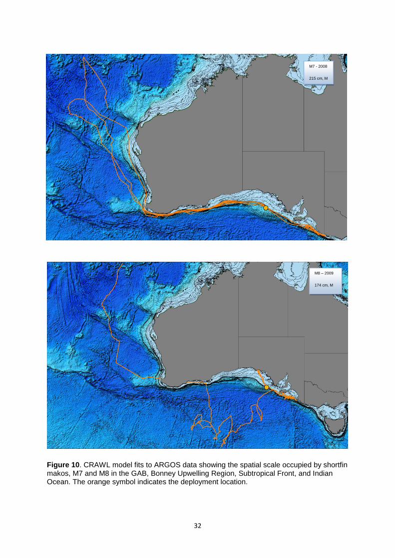
32
Figure 10. CRAWL model fits to ARGOS data showing the spatial scale occupied by shortfin makos, M7 and M8 in the GAB, Bonney Upwelling Region, Subtropical Front, and Indian Ocean. The orange symbol indicates the deployment location.
M7 - 2008
215 cm, M
M8 – 2009
174 cm, M
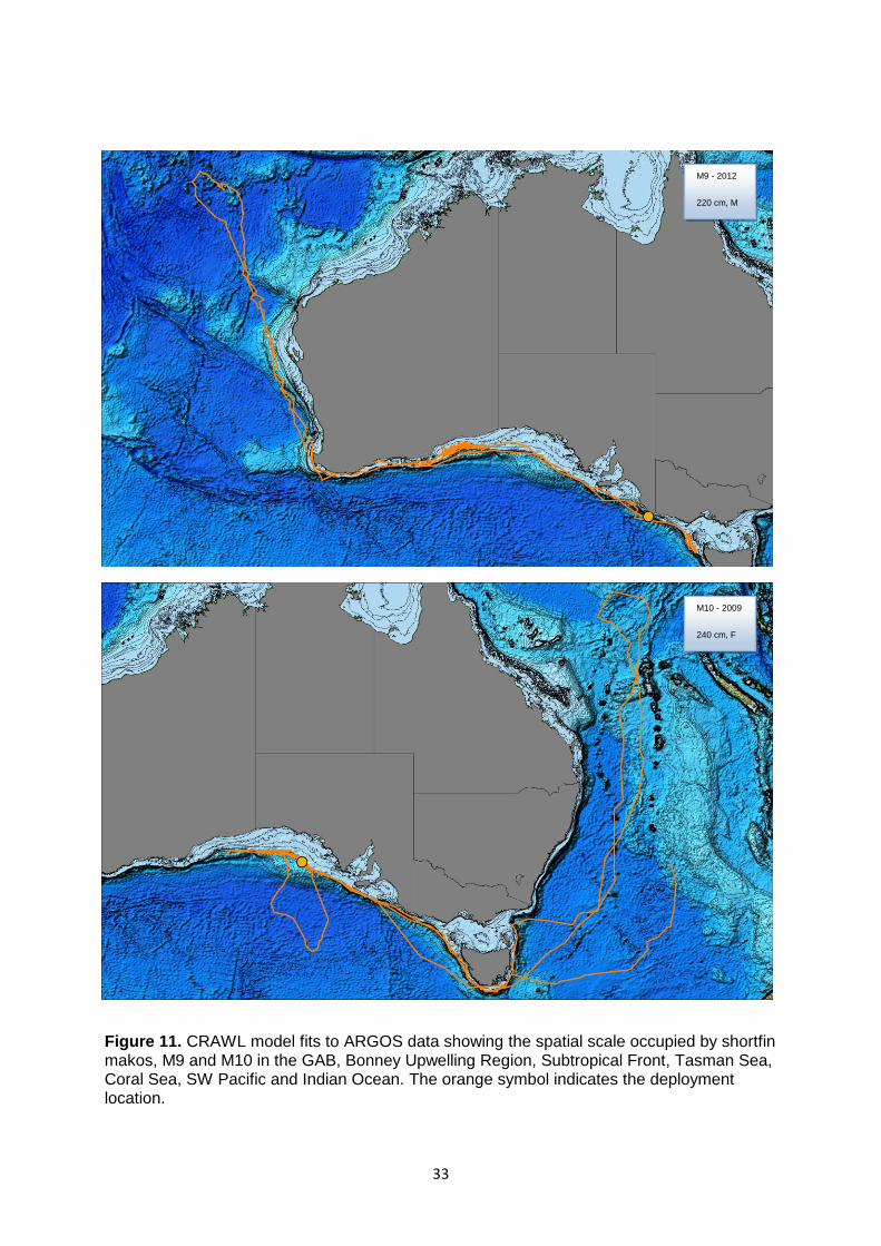
33
Figure 11. CRAWL model fits to ARGOS data showing the spatial scale occupied by shortfin makos, M9 and M10 in the GAB, Bonney Upwelling Region, Subtropical Front, Tasman Sea, Coral Sea, SW Pacific and Indian Ocean. The orange symbol indicates the deployment location.
M9 - 2012
220 cm, M
M10 - 2009
240 cm, F

34
Figure 12. CRAWL model fits to ARGOS data showing the spatial scale occupied by shortfin makos, M11 and M12 in the Bonney Upwelling Region, Tasman Sea, Coral Sea, SW Pacific, New Zealand shelf waters and New Caledonia. The orange symbol indicates the deployment location.
M11 - 2013
180 cm, F
M12 - 2013
187 cm, F

35
Figure 13. CRAWL model fit to ARGOS data showing the spatial scale occupied by shortfin mako M13 from the Bonney Upwelling Region across the GAB and during a trans-Indian Ocean migration. The orange symbol indicates the deployment location.
M13 - 2009
170 cm, M

36
Figure 14. CRAWL model fit to ARGOS data showing the spatial scale occupied by all shortfin makos M1–13 combined between 2008 and 2014.
37
Population genetics
Mitochondrial DNA sequence data - summary statistics and genetic diversity
The mitochondrial control region was sequenced for 365 shortfin makos resulting in 48
unique haplotypes, defined by 31 polymorphic sites (Table 3), which were sampled across
eight broad geographic regions encompassing 62 individual locations (Fig. 4).
Overall, haplotypic diversity was 0.894 ± 0.013 while nucleotide diversity was low at 0.004 ±
0.003. Population level measures of diversity, including sample size, number of haplotypes,
haplotypic and nucleotide diversity are shown in Table 3. Haplotypic and nucleotide
diversities per population ranged from 0.574 ± 0.067 to 0.940 ± 0.020 and 0.002 ± 0.001 to
0.005 ± 0.003, respectively, with averages of 0.875 ± 0.040 and 0.004 ± 0.002, respectively.
Mitochondrial DNA sequence data - Genealogical relationships
The haplotype network (Fig. 15) is dominated by a single, abundant haplotype that was
sampled in ~30% (108/365) of individuals, and from all locations. The network is diverse and
characterised by closely related haplotypes with most separated by only a single substitution.
Three substitutions was the maximum that was required to link any two haplotypes
parsimoniously. Although haplotype frequencies differ across sampling sites, the network
does not indicate any strong geographic partitioning of haplotypes. One third of haplotypes
(16/48) were unique to a single location, 13 of which were singletons (were only sampled
once), however most haplotypes are found at several, often geographically disparate
locations.
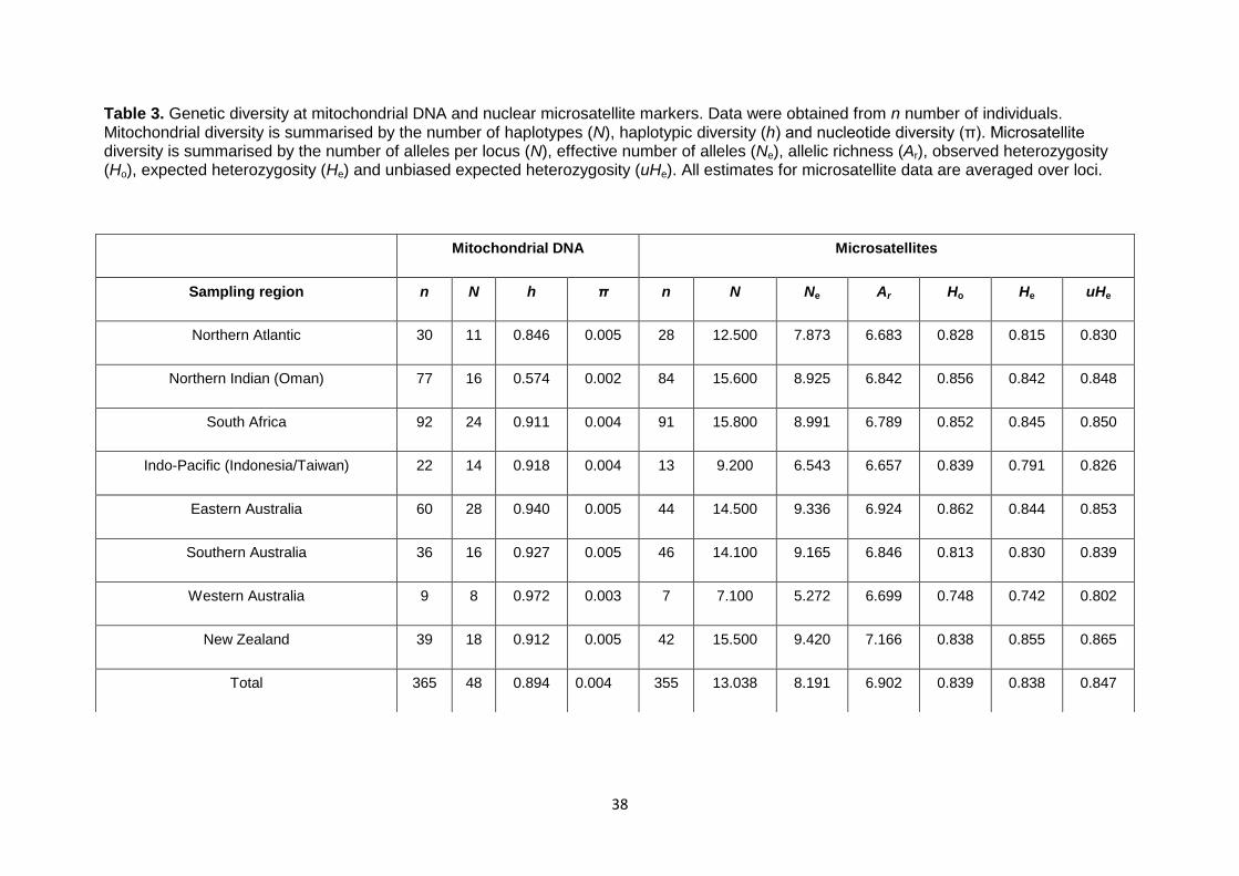
38
Table 3. Genetic diversity at mitochondrial DNA and nuclear microsatellite markers. Data were obtained from n number of individuals. Mitochondrial diversity is summarised by the number of haplotypes (N), haplotypic diversity (h) and nucleotide diversity (π). Microsatellite diversity is summarised by the number of alleles per locus (N), effective number of alleles (Ne), allelic richness (Ar), observed heterozygosity (Ho), expected heterozygosity (He) and unbiased expected heterozygosity (uHe). All estimates for microsatellite data are averaged over loci.
Mitochondrial DNA Microsatellites
Sampling region n N h π n N Ne Ar Ho He uHe
Northern Atlantic 30 11 0.846 0.005 28 12.500 7.873 6.683 0.828 0.815 0.830
Northern Indian (Oman) 77 16 0.574 0.002 84 15.600 8.925 6.842 0.856 0.842 0.848
South Africa 92 24 0.911 0.004 91 15.800 8.991 6.789 0.852 0.845 0.850
Indo-Pacific (Indonesia/Taiwan) 22 14 0.918 0.004 13 9.200 6.543 6.657 0.839 0.791 0.826
Eastern Australia 60 28 0.940 0.005 44 14.500 9.336 6.924 0.862 0.844 0.853
Southern Australia 36 16 0.927 0.005 46 14.100 9.165 6.846 0.813 0.830 0.839
Western Australia 9 8 0.972 0.003 7 7.100 5.272 6.699 0.748 0.742 0.802
New Zealand 39 18 0.912 0.005 42 15.500 9.420 7.166 0.838 0.855 0.865
Total 365 48 0.894 0.004 355 13.038 8.191 6.902 0.839 0.838 0.847
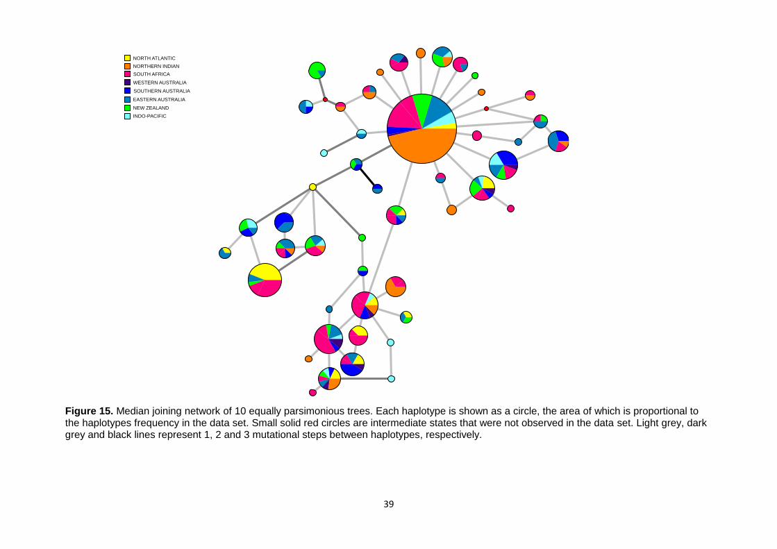
39
Figure 15. Median joining network of 10 equally parsimonious trees. Each haplotype is shown as a circle, the area of which is proportional to the haplotypes frequency in the data set. Small solid red circles are intermediate states that were not observed in the data set. Light grey, dark grey and black lines represent 1, 2 and 3 mutational steps between haplotypes, respectively.
NORTH ATLANTIC
SOUTHERN AUSTRALIA
SOUTH AFRICA
WESTERN AUSTRALIA
INDO-PACIFIC
EASTERN AUSTRALIA
NEW ZEALAND
NORTHERN INDIAN

40
Mitochondrial DNA sequence data – population differentiation
Pairwise fixation indices provide an indication of population differentiation, with an upper
ceiling of one that indicates complete differentiation (fixation for different alleles). Measures
of population differentiation may be based solely on differences in haplotype frequencies
among locations (FST). Alternatively, they may also incorporate additional information about
nucleotide diversity as an indication of haplotype similarity (ΦST). Both measures may be
susceptible to different biases depending on the proportion and patterns of shared diversity
among populations. It has thus become common practice to report both metrics (Bird et al.
2011, Holsinger et al. 2009). Values of FST and ΦST were low to moderate. Both Northern
Hemisphere locations (Northern Atlantic and Northern Indian Ocean) were significantly
differentiated from all Southern Hemisphere localities based on FST, ΦST and exact tests of
population differentiation (Table 4). Weak but significant differentiation was detected
between South Africa and southern Australia based on FST, but not between South Africa
and any other Australasian location (eastern Australia or New Zealand.). This result was not
corroborated by ΦST estimates in which South Africa was not significantly differentiated from
any of the Australasian locations (southern Australia, eastern Australia or New Zealand.).
Conversely, South Africa was significantly differentiated from all other locations based on
exact tests of population differentiation (Table 4). Within Australasia, significant
differentiation was detected between southern Australia and New Zealand based on FST, ΦST
and exact tests of population differentiation (Table 4).
Population differentiation was also assessed using Analysis of Molecular Variance (AMOVA).
Interpretations presented herein are based on ΦST, but results from AMOVA based on FST
were qualitatively similar. The global ΦST estimate was low (ΦST = 0.080), but significant (P =
0.000). Total variation in the data set could be separated into five major regions: the northern
Atlantic, the northern Indian, South Africa, western Australasia (western and southern
Australia) and eastern Australasia (Indo-Pacific, eastern Australia and New Zealand). While
most of the variation in the data set was found within populations (91.5%, FST = 0.085, P =
0.000), among region variance accounted for a significant 8.2% (FCT = 0.082, P = 0.009) of
the total variation. Partitioning among regions was weaker (2.0%) when considering only
South Africa and the Australasian locations (South Africa vs. western Australasia (western
and southern Australia) vs. eastern Australasia (Indo-Pacific, eastern Australia and New
Zealand)), although still significant (FCT = 0.020, P = 0.032). However, the among-region
variance component was not significant (FCT = -0.006, P = 0.666) in an AMOVA on data in
which all Australasian locations were grouped together (South Africa vs. western, southern
and eastern Australia, Indo-Pacific and New Zealand). The global ΦST was non-significant
41
(1.63% of total variation, ΦST = 0.016, P=0.06) when considering all sampling locations in
Australasia (Indo-Pacific, eastern Australia, western Australia, southern Australia and New
Zealand). Similarly, there was no significant difference (3.5% of total variation, ΦCT = 0.035,
P = 0.100) between regions when partitioning the data set into eastern (Indo-Pacific, eastern
Australia, New Zealand) and western (western Australia, southern Australia) Australasia.
Nuclear microsatellite DNA data - summary statistics and genetic diversity
Ten microsatellite loci were genotyped for 355 shortfin makos sampled across the eight
broad geographic locations (Fig. 4, Table 3). There was no evidence of scoring errors due to
short allele dominance or typographic error. Two loci, Iox-12 and Iox-D123, showed evidence
of null alleles. These were in low frequency (<10% based on all estimators; Van Oosterhout
et al. 2004), detected in samples from a single location and due to significant excess of
homozygotes observed in two and one genotype classes respectively. Following Bonferroni
correction, all loci and populations conformed to expectations under a model of Hardy-
Weinberg equilibrium. These loci therefore, were not excluded from further analyses.
Linkage disequilibrium was detected for three locus pairs (Iox-M110 and Iox-B3, Iox-12 and
Iox-30, Iox-M192 and Iox-D123), however these results too could be accounted for by
significant comparisons in single sampling locations and so were not excluded from final
analyses.
Genetic diversity at microsatellite loci was moderate to high. The number of alleles per locus
(N) ranged between 9 and 30, with means per population ranging from 7.10 to 15.80 (Table
3). The effective number of alleles per locus ranged between 5.27 and 9.42 across
populations. Allelic richness was relatively consistent across populations, ranging between
6.66 and 7.17. Unbiased expected heterozygosity was also relatively consistent across
populations, ranging between 0.80 and 0.87. Observed heterozygosity ranged from 0.75 to
0.86 (Table3). Lower sample sizes from western Australia and the Indo-Pacific resulted in
slightly reduced diversity (Table 3) and greater divergence between expected and observed
heterozygosities.

42
Table 4. Pairwise measures of population differentiation based on mitochondrial DNA. FST values are below the diagonal and ΦST values are
above the diagonal. Significance was assessed using a non-parametric permutation approach. * indicates a comparison that represents significant differentiation at the 95% confidence level following Bonferroni correction. Exact tests of population differentiation were also conducted. λ in the lower diagonal of the matrix indicates resultant significant comparisons.
northern northern South eastern southern New
Atlantic Indian Africa Australia Australia Zealand
northern Atlantic 0.396* 0.114
* 0.139
* 0.147
* 0.152
*
northern Indian 0.257λ*
0.100* 0.073
* 0.186
* 0.077
*
South Africa 0.041λ*
0.119λ*
0.004 0.027 0.020
eastern Australia 0.072λ*
0.109λ*
0.007λ 0.021 0.002
southern Australia 0.080λ*
0.197λ*
0.029λ*
0.011 0.063*
New Zealand 0.077λ*
0.115λ*
0.016λ -0.002 0.032
λ*

43
Nuclear microsatellite DNA data – population differentiation
As was the case when estimating population differentiation based on mitochondrial DNA,
measures of population differentiation based on microsatellite data may be based on allelic
frequency differences among locations (FST) or also incorporate information about the
evolutionary distance between alleles (RST). The majority of the variation in the microsatellite
data occurred within populations (99.9%) and the global multilocus FST (considering samples
from all locations across both hemispheres) estimate was low (FST = 0.002), but marginally
significant (P = 0.020). Individual locus FST estimates were low, ranging between -0.003 and
0.009. The significant multilocus FST result was driven by significant FST values at just two of
the 10 loci (Iox-M192, FST = 0.005, P = 0.004; Iox-M36 FST = 0.009, P = 0.001). The
multilocus RST estimate was also low (RST = 0.002) but non-significant (P = 0.250).
The same population pairwise comparisons as were performed for the mitochondrial data
were also made for the microsatellite data. Somewhat contrasting the results from mtDNA
where significant differentiation was detected when comparing northern and southern
hemisphere, for the microsatellite data all population pairwise estimates of GST and GST’’
were low and only a single pairwise comparison, that between South Africa and southern
Australia, indicated significant differentiation (Table 5). Significant divergence between South
Africa and southern Australia however, was not supported by AMOVA of microsatellite data.
When partitioning the data by region, ie. northern Atlantic vs. northern Indian vs. South
Africa vs. Australasia (eastern Australia, southern Australia and New Zealand grouped
together), the among-region variance component was non-significant, accounting for < 1% of
total variation in the dataset (FCT = 0.002, P = 0.196). Likewise, the among-population
component was also non-significant (FSC = 0.001, P = 0.623). The majority (99.8%) of
variation was found within populations. This result was consistent across AMOVA analyses
based on allelic (FST) and genotypic (RST) data, thus only the results from the allelic-based
analysis are presented.
Fig. 16 shows the statistical power of our microsatellite data, given the sample sizes, number
of loci, and average allele frequencies characterizing our empirical data set, to detect various
levels of true population differentiation (FST). Our data set has good statistical power with a
100% probability of detecting a true FST as low as 0.0025 and a high probability (65 – 70%)
of detecting an FST as low as 0.001. The alpha error (corresponding to the probability of
obtaining false significances when the true FST = 0) was ≤ 5%.

44
Figure 16. Statistical power of microsatellite data to detect various levels of true population differentiation (FST).
Model-based clustering analyses performed in Structure also indicated high connectivity
among all sampling locations (Fig. 17). The mean estimated log probability of the data was
highest for K = 1, while the modal value of the distribution of ∆K (Evanno et al. 2005)
suggested that 2 clusters could be identified in the data. The ∆K metric cannot be estimated
for K=1 and so panmixia could not be assessed as a possible scenario using this approach.
Further, this metric does not take into account the scale of ∆K. We observed values that
were two orders of magnitude smaller than is typically observed for cases of real structure. In
addition, the bar plots of the estimated cluster membership coefficients for each individual
did not show support for K = 2. Although subtle differences in allele frequencies were
detected across sampling sites, individuals were assigned in similar proportions to each of
the two clusters (Fig. 17). There was considerable variance in parameter estimates across
runs for each individual K, which indicates non-convergence of the analysis despite running
for a sufficient length of time. Together these observations are consistent with there being
little to no signal of population structure in the data.

45
Table 5. Pairwise measures of population differentiation based on nuclear microsatellite data. GST values are below the diagonal and GST
’’
values are above the diagonal. Significance was assessed using a non-parametric permutation approach. Populations that were significantly differentiated at the 95% confidence level, following Bonferroni correction for multiple comparisons, are indicated by an *.
northern northern South eastern southern New
Atlantic Indian Africa Australia Australia Zealand
northern Atlantic 0.017 0.025 0.008 0.031 0.017
northern Indian 0.001 0.016 0.007 0.015 0.015
South Africa 0.002 0.001 0.016 0.043* 0.011
eastern Australia 0.001 0.001 0.001 0.000 -0.005
southern Australia 0.003 0.001 0.003* 0.000 0.025
New Zealand 0.001 0.001 0.001 0.000 0.002
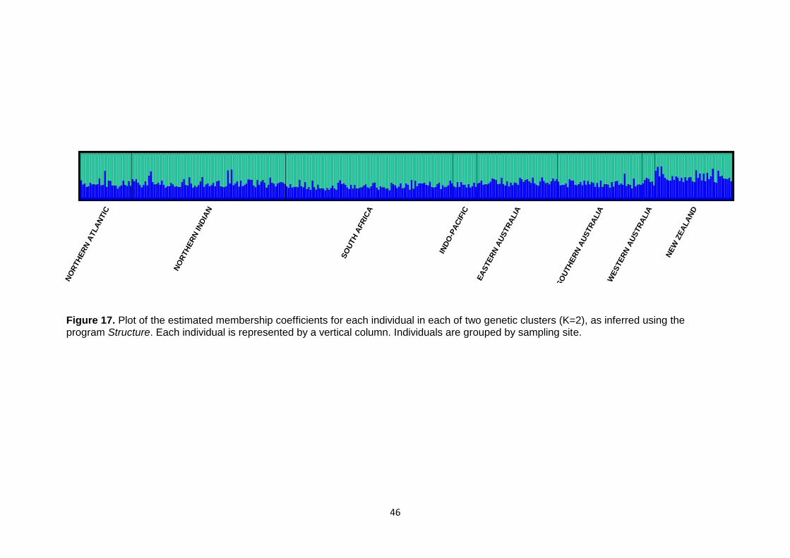
46
Figure 17. Plot of the estimated membership coefficients for each individual in each of two genetic clusters (K=2), as inferred using the program Structure. Each individual is represented by a vertical column. Individuals are grouped by sampling site.
NO
RTH
ER
N A
TLA
NTIC
NO
RTH
ER
N IN
DIA
N
SO
UTH
AFR
ICA
IND
O-P
AC
IFIC
EA
STE
RN
AU
STR
ALIA
SO
UTH
ER
N A
US
TR
ALIA
WE
STE
RN
AU
STR
ALIA
NE
W Z
EA
LA
ND

47
Nuclear microsatellite DNA data – sex-biased dispersal
Pairwise fixation indices were higher between sampling locations for mitochondrial DNA
markers than for microsatellite markers, however this is expected given the four-fold lower
effective population size of mitochondrial DNA relative to nuclear DNA. There were no
obvious differences in patterns of differentiation when comparing males and females of
either marker type (Table 6). Fixation indices for both marker types were generally low in
both sexes, however Pairwise estimates of ΦST were usually (although not always) higher in
females than in males for mitochondrial DNA (Table 6a). This pattern was not observed in
the microsatellite data (Table 6b). FST and relatedness based on microsatellite markers were
both low overall, but higher in females (FST = 0.003, r = 0.006, respectively) than in males
(FST = 0.000, r = -0.001). This difference bordered on significance (P = ~ 0.050), however the
observed values of the test statistics for these parameters were within the range of the null
distribution that dispersal is independent of sex (Figure 18). FIS was higher in males (FIS =
0.009) than females (FIS = 0.001) but this difference was not significant (P = 0.203, Table 7,
Figure 18). Corrected assignment (AIc) values ranged between −8.01 and 7.94 for males and
−6.23 and 10.78 for females (Figure 18). Mean AIc was higher for females (0.190) than for
males (-0.191), however this difference was not statistically significant (P = 0.158, Table 7).
Variance of AIc was also higher for females (11.865) than for males (9.112) but this
difference was also not significant (P = 0.838, Table 7). The observed value of the test
statistics for both the mean and variance of AIc fell within the range of the null distribution
representing the probability that dispersal is unbiased by sex (Fig. 18). The frequency
distributions of AIc values for males and females were largely overlapping (Fig. 18) and both
sexes showed a similar proportion of values in the negative portion of the distribution (54%
for females and 52% for males).
Spatial patterns of genetic structure were similar across sexes (Fig. 19). The null hypothesis
of correlogram homogeneity across sexes was accepted in all three heterogeneity tests. The
male and female 95% bootstrap confidence intervals about r overlapped in all distance
classes (Fig. 19). The single distance class t2 tests were all non-significant (Table 8), as was
the multi-class ω test of overall correlogram heterogeneity (ω = 6.226, P = 0.411). Significant
departure from the null of hypothesis of randomly distributed genotypes in space was
detected for both males and females with low but significant positive autocorrelation among
genotypes detected at small (100 km) distance classes (rMALES = 0.009, P = 0.000; rFEMALES =
0.008, P = 0.003 for the first distance class; ωMALES = 59.401, P = 0.000; ωFEMALES = 33.078,
P = 0.007; Table 8; Fig. 19).
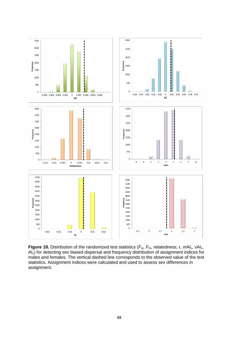
48
Figure 18. Distribution of the randomized test statistics (Fst, FIS, relatedness, r, mAIc, vAIc, AIc) for detecting sex biased dispersal and frequency distribution of assignment indices for males and females. The vertical dashed line corresponds to the observed value of the test statistics. Assignment Indices were calculated and used to assess sex differences in assignment.

49
Figure 19. Correlogram plots of the spatial autocorrelation coefficient, r as a function of geographical distance for males (in blue) and females (in red). Upper and lower bounds for the 95% confidence interval for the null hypothesis of no spatial structure (r = 0) based on 10, 000 random permutations of the data among distance classes are depicted as black dotted lines. 95% confidence intervals about r were determined using 10, 000 bootstrap replicates. Geographic distances (km) presented are the maximum distance of each class.

50
Table 6. Comparisons of pairwise measures of population differentiation for females (below diagonal) and males (above diagonal) based on ΦST values for mitochondrial DNA (a) and GST
’’ values for nuclear microsatellite data (b). Significance was assessed using a non-parametric
permutation approach. Populations that were significantly differentiated at the 95% confidence level, following Bonferroni correction for multiple comparisons are represented using a superscripted star (*)
(a) northern South eastern southern New
Indian Africa Australia Australia Zealand
northern Indian 0.082* 0.079
* 0.168
* 0.098
South Africa 0.168* 0.002 0.015 0.008
eastern Australia 0.135* -0.001 -0.005 -0.0161
southern Australia 0.205* 0.051
* 0.012 0.016
New Zealand 0.130* 0.020 -0.006 0.028
(b) Northern South Eastern Southern New
Indian Africa Australia Australia Zealand
northern Indian 0.005 0.010 0.008 0.017
South Africa 0.009 0.009 0.009 0.015
eastern Australia 0.009 0.010 0.010 0.017
southern Australia 0.009 0.014 0.012 0.020
New Zealand 0.010 0.009 0.008 0.014

51
Table 7. F-statistics, relatedness (r), mean assignment (mAIC) and variance assignment (vAIC) for each sex. Significance was assessed using
the randomisation method.
FST
r FIS
mAIC vAI
C
Males -0.0004 -0.0007 0.0092 -0.1914 11.8649
Females 0.0029 0.0059 0.0010 0.1901 9.1119
P-value 0.0510 0.0501 0.2033 0.1578 0.8376

52
Table 8. Tests of spatial autocorrelation and among sex correlogram heterogeneity. Numbers of comparisons (n), autocorrelation coefficients, r and P-values are shown for each distance class as well as a multiclass test criterion (ω) of the departure from the null hypothesis of r = 0.
Single-class (t2) and multiclass (ω) test criteria and associated P-values for the test of correlogram homogeneity across sexes are also shown.
Distance class (km)
Spatial autocorrelation 100 1500 3000 6500 10000 15000 ω test P-value
Males n 2851 366 407 170 2773 4608 59.401 0.000
r 0.009 0.011 0.006 -0.017 -0.006 -0.003
P-value 0.000 0.019 0.112 0.979 0.999 0.977
Females n 2851 366 407 170 2773 4608 33.078 0.007
r 0.008 0.002 0.000 0.001 -0.003 -0.002
P-value 0.003 0.396 0.592 0.219 0.997 0.725
Among sex heterogeneity ω test P-value
t2 0.062 1.401 0.836 2.977 0.703 0.031 6.226 0.411
P-value 0.800 0.237 0.362 0.084 0.398 0.862
53
Effective population size estimates
Applying CNe crit values within the range of acceptable bias-precision trade-off (0.020 < Pcrit <
0.050) resulted in finite point estimates of CNe for most sampling locations, ranging in order
of magnitude from hundreds to several thousand (Table 9). A finite estimate could not be
obtained for eastern Australia. Negative estimates of CNe were obtained for this location
across a range of Pcrit values (0.020 – 0.20). The lower bounds of the 95% confidence
intervals were in the hundreds for all locations (except eastern Australia which was
unbounded), while upper bounds were mostly infinite (Table 9). Estimated effective
population size for the Australasian region (Indo-Pacific, eastern, southern, and western
Australia and New Zealand) was 2,550.6 (95% CI = 831, ∞). An infinite measure of CNe is an
artefact of the linkage disequilibrium method used here and essentially an indication of
insufficient power due to various biases and difficulties, that are well documented in the
literature (Luikart et al. 2010, Waples and Do 2010, Hare et al. 2011), associated with
estimating CNe in large populations of highly diverse animals with overlapping generations.
Since populations cannot be infinite in size, these estimates are more appropriately reported
as inestimable in Table 9. Finite lower and upper bounds on the 95% confidence interval
surrounding the estimate were only obtained for the northern Indian location. Population size
was comparatively small at this location with a point estimate of 252.3. The lower and upper
bounds were 169.6 and 465.4, respectively (Table 9).

54
Table 9. Estimates of effective population size (CNe) and associated upper and lower bounds of the 95% confidence interval (CI). Bias-precision trade-off is most balanced when using allele frequency exclusion criterions (Pcrit) within the range 0.02 to 0.05.
Regions Sample size CNe 95% CI lower 95% CI upper Pcrit
northern Atlantic 28 1208.8 109.1 inestimable 0.04
northern Indian 84 252.3 169.6 465.4 0.02
South Africa 91 1409.9 413.7 inestimable 0.03
eastern Australia 57 Infinitely large inestimable inestimable 0.02 – 0.2
southern Australia 53 5692.5 368.7 inestimable 0.02
New Zealand 42 566.6 203.8 inestimable 0.02
Australasian (eastern Australia, southern Australia, New Zealand) 152 2550.6 831 inestimable 0.02

55
Discussion
During this study, we investigated the population structure and movement patterns of shortfin
mako populations in the Australasian and central Indo-Pacific using conventional tagging, long-
term satellite telemetry, mitochondrial DNA and nuclear DNA datasets. We provide high-resolution
information regarding the spatial connectivity of shortfin mako populations in the Australasian and
Central Indo-Pacific Region that can inform discussions regarding regional-scale management
options for this species.
Although genetic population structure has been investigated previously for the shortfin mako, all
prior studies have largely addressed differentiation at the inter-oceanic scale, with a focus on the
Pacific Ocean basin. Sampling from the Australasian region has been limited and prohibited
assessments at scales suitable for informing fishery management decisions within the Australian
Exclusive Economic Zone. Additionally, sampling of shortfin makos in the Southern and Indian
Ocean basins was particularly sparse prior to this study, limiting our ability to make inferences
about connectivity between Australasian and neighbouring populations. Previous studies of the
movement of this species using tracking data have mostly focused on the southwest Pacific
Ocean off eastern Australia and sample sizes were relatively small (e.g. Stevens et al. 2010). This
study represents the first multidisciplinary study of the movement and population connectivity of
the shortfin mako throughout the Australasian region, using information from both genetic and
tracking datasets and including representatives from the Indian Ocean, allowing these factors to
be more rigorously assessed.
Matrilineal population differentiation
There have been three prior studies of population genetic structure based on mitochondrial DNA in
shortfin mako (Heist et al. 1996; Taguchi et al 2011; Michaud et al. 2011). Divergence between the
Atlantic and Pacific Ocean basins was a common result in all of these studies, as well as evidence
of reduced cross-equatorial connectivity. While Heist et al. (1996) and Taguchi et al. (2011) were
unable to distinguish north and south Pacific sampling sites, improved sampling (840 individuals
from five regions in the Pacific, and one in the Atlantic Ocean) by Michaud et al. (2011) revealed
significant differences between the north and south Pacific, and the southeast and southwest
Pacific. Taguchi et al. (2011) was the only one of these studies to consider samples from the
Indian Ocean. The eastern Indian Ocean was found to be divergent from all sampling sites, except
the north Atlantic. This included significant differentiation between the eastern Indian Ocean and
east coast of Australia, indicating possible east-west matrilineal population structure in the shortfin
mako in Australian waters. However, sparse sampling of highly genetically diverse, mobile animals

56
can easily lead to frequency differences that give a falsely inflated sense of population structure,
and therefore these patterns must be interpreted with caution given the relatively small sample
sizes analysed by Taguchi et al. (2011).
Similar to previous studies (Heist et al. 1996; Taguchi et al. 2011), we found considerable
mitochondrial DNA genetic diversity in shortfin makos. Haplotypic diversity was higher than 0.9 at
most sampling sites (Fig. 15, Table 3), which is toward the higher end of the range typically found
for elasmobranchs (Hoelzel et al. 2006; Keeney and Heist 2006; Castro et al. 2007; Dudgeon et al.
2008; Schultz et al. 2008; Chabot and Allen 2009; Benavides et al. 2011; Blower et al. 2012) and
typical of other highly mobile pelagic species (Graves 1998). Also consistent with previous work,
our mitochondrial DNA data set showed little evidence of trans-equatorial migration. Both Northern
Hemisphere sampling locations (north Atlantic and northern Indian) were significantly differentiated
from all other sampling sites (Table 4). We were unable to distinguish the Indo Pacific sampling
site from those in the Australian region, however this sample included just five individuals sampled
from the Northern Hemisphere. The majority of samples included in the Indo Pacific site were
sampled from fish markets in Indonesia, and were likely caught in the Southern Hemisphere. Our
data, therefore, does not allow a comprehensive assessment of trans-equatorial gene flow
between Australian populations and those in the northern Pacific however, Michaud et al. (2011)
describe significant differentiation between the northwest and southwest Pacific, indicating that
trans-equatorial migration is similarly limited in this region.
Michaud et al. (2011) hypothesised that haplotype sharing between the Atlantic and Australia/New
Zealand indicates that gene flow between the Pacific and Atlantic populations, occurs primarily
through the Indian Ocean. Limited sampling from both the Indian Ocean and Australasian region
prevented further investigation in their study. Our analyses provide some support for this
hypothesis, as we did not distinguish South Africa from the Australasian populations and all
pairwise fixation indices involving comparisons between these two regions were low relative to
comparisons between Northern and Southern Hemisphere sampling sites. All pairwise ΦST
estimates between South Africa and the Australasian region were non-significant, indicating that
gene flow occurs across the Indian Ocean (Table 4). This result is consistent with Taguchi et al.
(2011) who could not distinguish western Indian Ocean sampling sites from those in the eastern
Indian Ocean, or the Pacific Ocean. Our exact tests of population differentiation, however,
indicated significant differentiation between Australasian and South African sampling sites, and a
single pairwise comparison between South Africa and southern Australia was also significant
based on FST (Table 4). These significant comparisons should be interpreted with caution,
however, given the small magnitude of observed pairwise fixation indices. The frequency data
inherent in the analysis of population structure is particularly susceptible to noise due to random
sampling error both at the intralocus (number of individuals) and interlocus (number of loci
sampled) levels. This is exacerbated in high gene flow species, such as shortfin mako, such that it
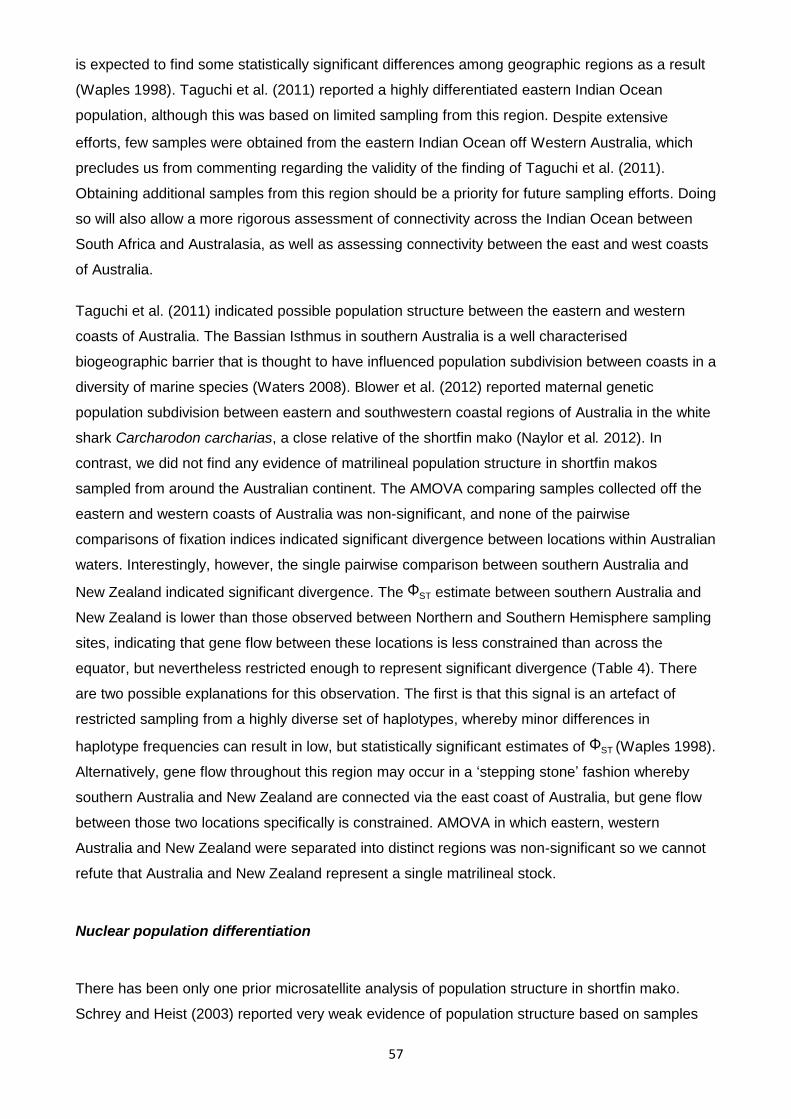
57
is expected to find some statistically significant differences among geographic regions as a result
(Waples 1998). Taguchi et al. (2011) reported a highly differentiated eastern Indian Ocean
population, although this was based on limited sampling from this region. Despite extensive
efforts, few samples were obtained from the eastern Indian Ocean off Western Australia, which
precludes us from commenting regarding the validity of the finding of Taguchi et al. (2011).
Obtaining additional samples from this region should be a priority for future sampling efforts. Doing
so will also allow a more rigorous assessment of connectivity across the Indian Ocean between
South Africa and Australasia, as well as assessing connectivity between the east and west coasts
of Australia.
Taguchi et al. (2011) indicated possible population structure between the eastern and western
coasts of Australia. The Bassian Isthmus in southern Australia is a well characterised
biogeographic barrier that is thought to have influenced population subdivision between coasts in a
diversity of marine species (Waters 2008). Blower et al. (2012) reported maternal genetic
population subdivision between eastern and southwestern coastal regions of Australia in the white
shark Carcharodon carcharias, a close relative of the shortfin mako (Naylor et al. 2012). In
contrast, we did not find any evidence of matrilineal population structure in shortfin makos
sampled from around the Australian continent. The AMOVA comparing samples collected off the
eastern and western coasts of Australia was non-significant, and none of the pairwise
comparisons of fixation indices indicated significant divergence between locations within Australian
waters. Interestingly, however, the single pairwise comparison between southern Australia and
New Zealand indicated significant divergence. The ΦST estimate between southern Australia and
New Zealand is lower than those observed between Northern and Southern Hemisphere sampling
sites, indicating that gene flow between these locations is less constrained than across the
equator, but nevertheless restricted enough to represent significant divergence (Table 4). There
are two possible explanations for this observation. The first is that this signal is an artefact of
restricted sampling from a highly diverse set of haplotypes, whereby minor differences in
haplotype frequencies can result in low, but statistically significant estimates of ΦST (Waples 1998).
Alternatively, gene flow throughout this region may occur in a ‘stepping stone’ fashion whereby
southern Australia and New Zealand are connected via the east coast of Australia, but gene flow
between those two locations specifically is constrained. AMOVA in which eastern, western
Australia and New Zealand were separated into distinct regions was non-significant so we cannot
refute that Australia and New Zealand represent a single matrilineal stock.
Nuclear population differentiation
There has been only one prior microsatellite analysis of population structure in shortfin mako.
Schrey and Heist (2003) reported very weak evidence of population structure based on samples
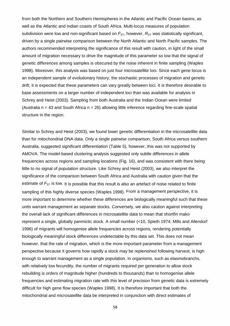
58
from both the Northern and Southern Hemispheres in the Atlantic and Pacific Ocean basins, as
well as the Atlantic and Indian coasts of South Africa. Multi-locus measures of population
subdivision were low and non-significant based on FST, however, RST was statistically significant,
driven by a single pairwise comparison between the North Atlantic and North Pacific samples. The
authors recommended interpreting the significance of this result with caution, in light of the small
amount of migration necessary to drive the magnitude of this parameter so low that the signal of
genetic differences among samples is obscured by the noise inherent in finite sampling (Waples
1998). Moreover, this analysis was based on just four microsatellite loci. Since each gene locus is
an independent sample of evolutionary history, the stochastic processes of migration and genetic
drift, it is expected that these parameters can vary greatly between loci. It is therefore desirable to
base assessments on a larger number of independent loci than was available for analysis in
Schrey and Heist (2003). Sampling from both Australia and the Indian Ocean were limited
(Australia n = 43 and South Africa n = 26) allowing little inference regarding fine-scale spatial
structure in the region.
Similar to Schrey and Heist (2003), we found lower genetic differentiation in the microsatellite data
than for mitochondrial DNA data. Only a single pairwise comparison, South Africa versus southern
Australia, suggested significant differentiation (Table 5), however, this was not supported by
AMOVA. The model-based clustering analysis suggested only subtle differences in allele
frequencies across regions and sampling locations (Fig. 16), and was consistent with there being
little to no signal of population structure. Like Schrey and Heist (2003), we also interpret the
significance of the comparison between South Africa and Australia with caution given that the
estimate of FST is low. It is possible that this result is also an artefact of noise related to finite
sampling of this highly diverse species (Waples 1998). From a management perspective, it is
more important to determine whether these differences are biologically meaningful such that these
units warrant management as separate stocks. Conversely, we also caution against interpreting
the overall lack of significant differences in microsatellite data to mean that shortfin mako
represent a single, globally panmictic stock. A small number (<10, Spieth 1974; Mills and Allendorf
1996) of migrants will homogenise allele frequencies across regions, rendering potentially
biologically meaningful stock differences undetectable by this data set. This does not mean
however, that the rate of migration, which is the more important parameter from a management
perspective because it governs how rapidly a stock may be replenished following harvest, is high
enough to warrant management as a single population. In organisms, such as elasmobranchs,
with relatively low fecundity, the number of migrants required per generation to allow stock
rebuilding is orders of magnitude higher (hundreds to thousands) than to homogenise allele
frequencies and estimating migration rate with this level of precision from genetic data is extremely
difficult for high gene flow species (Waples 1998). It is therefore important that both the
mitochondrial and microsatellite data be interpreted in conjunction with direct estimates of

59
dispersal via tracking studies to delineate population structure in high gene flow species such as
the shortfin mako. Essentially, genetic data offer an across generation estimation of the extent of
movement via gene flow. Tracking data provides a within-lifetime estimate of movement and
combining the two can better elucidate whether a signal of panmixia is likely driven by few,
relatively rare dispersal events or whether a species is highly vagile, promoting high connectivity
between locations. Combining the two data types can also reveal patterns that may have been
overlooked if relying solely on one data type. For example, a signature of reproductive philopatry
may be overlooked in wide ranging animals if individuals are sampled for genetic analysis during
the dispersed phase, which would promote an artificial signature of panmixia.
Sex-biased dispersal
Sex-biased dispersal is a pattern where individuals of one sex remain philopatric to a particular site
for breeding, while those of the opposite sex disperse. Generally, dispersal tends to be male-
biased with polygynous breeding systems such as mammals, while female-biased dispersal is
predicted for monogamous systems, e.g. birds (Greenwood 1980). It is important to identify and
manage species that exhibit sex-biased dispersal accordingly to avoid selective overharvest of the
more philopatric sex, if fishing practices are concentrated in their comparatively smaller range.
Furthermore, identifying areas to which females exhibit philopatry can aid in locating pupping and
nursery grounds (Hueter 1998). Male-biased dispersal has been demonstrated in a number of
elasmobranch species (Keeney et al. 2003; Keeney et al. 2005; Duncan et al. 2006; Schultz et al.
2008; Daly-Engel et al. 2012) including the white shark (Pardini et al. 2001; Blower et al. 2012),
which also shows trans-oceanic migrations by both sexes (Bonfil et al. 2005; Bruce et al. 2006).
Schrey and Heist (2003) suggested sex-biased dispersal as a possible mechanism to explain the
magnitude of the difference in degree of genetic structure inferred from mitochondrial DNA and
microsatellite markers between ocean basins in shortfin mako (mitochondrial DNA is maternally
inherited and therefore strong mitochondrial structure in the absence of microsatellite structure can
indicate female philopatry). Sexual segregation, based on sex-ratios of catches in high seas long-
line fishery bycatch data has also been identified for shortfin makos in the South-east Pacific
Ocean, with females found in higher frequencies with increasing proximity to the South American
continent (Mucienties et al. 2009). However, an observer program in the ETBF in the SW Pacific
found that for 1,126 shortfin makos for which sex was determined, 42% were male, and 58% were
female (Bruce 2014), and both regional and seasonal differences were apparent in proportions of
sexes in observer based monitoring of pelagic long-line catches off New Zealand (Francis 2013).
Together these studies indicate that shortfin makos exhibit some degree of female philopatry,
however, how best to integrate this information with current management strategies and Recovery
Plans remains unclear. As with all HMS, it is difficult to distinguish movements for breeding that
have genetic consequences and implications for long-term population dynamics and survival, from

60
other types of movement. Our data suggests a trend toward male-biased dispersal, although for
the most part this observation was not statistically supported. Fixation indices were higher for
mitochondrial DNA than for microsatellite markers and the magnitude of this difference exceeds
the expectation if it were driven only by differences in the relative effective population sizes of
these two markers (Table 4 and Table 5). Pairwise estimates of ΦST were usually higher in
females than in males for mitochondrial DNA (Table 6a), although this pattern was not observed in
the microsatellite data (Table 6b). Sample sizes are reduced further in analyses that are split by
sex and therefore the significance of these results must be interpreted with caution for reasons
that were outlined previously.
Allele frequencies across sampling sites should be more similar for individuals of the dispersing
sex than those of the more philopatric sex. The expectation therefore, is for FST and relatedness (r)
to be highest in the more philopatric sex. Additionally, because the dispersing sex should largely
consist of immigrant and less related individuals, we expect them to have a lower probability of
local assignment and greater variance in assignment index than the philopatric sex (Goudet et al.
2002). The observed values for these parameters (Table 7) in this study were consistent with
these expectations, indicating male-biased dispersal in shortfin mako. However, the test statistics
based on the difference in these parameters between sexes fell within the randomised distribution
representing the null hypothesis of no sex-biased dispersal (Fig.18).
There are several caveats to the interpretation of these results. These tests lack power to detect
sex-biased dispersal unless the bias is very strong (> 80:20) and dispersal occurs at intermediate
rates (Goudet et al. 2002). It is highly possible that our analyses are lacking in power due to both
of these factors. Both tracking data and the low observed fixation indices based on genetic data
suggest that both male and female shortfin mako are highly mobile. If females exhibit philopatry it
seems more likely that this will be towards generalised oceanic areas, rather than discrete pupping
grounds, both of which indicate that any bias that may exist is likely to be weak and operating at
the ocean basin scale (i.e. females are philopatric to particular ocean basins, but not to discrete
sites within them). Moreover, this high mobility and genetic diversity observed in the shortfin mako
implies that populations are likely to be large and diffuse. In turn, this implies that very large
sample sizes will be required to estimate allele frequencies with sufficient precision to detect
immigrant genotypes. Finally, these tests are only applicable if dispersal occurs prior to
reproduction and sampling occurs after dispersal (Goudet et al. 2002). This prerequisite is
extremely difficult to ensure in HMS. Mature shortfin mako are generally rare, such that our
sample consists of a mixture of mostly juvenile and sub-adult individuals sampled over several
years from multiple cohorts. It is possible that this unavoidable sampling scheme is masking any
signal of statistically supported sex-biased dispersal in these particular analyses, although the
trend indicates a male-bias.

61
We did not detect any differences in spatial genetic structure across sexes based on the spatial
autocorrelation analysis. Ability to detect a sex bias using this method is also highly dependent
upon sample size and requires the development of strong spatial genetic structure in the more
philopatric sex before a difference will be rendered statistically significant (Smouse et al. 2008;
Banks and Peakall 2012), which is unlikely to occur in HMS. Although we detected low, but
significant positive autocorrelation among genotypes at small distance classes, the magnitude of
autocorrelation was similar in males and females and bootstrap confidence intervals were
overlapping. Banks and Peakall (2012) stressed the importance of sampling at or below the scale
at which dispersal is restricted in the more philopatric sex in order to concentrate pairwise data
points at that spatial scale. This analysis and our inferences regarding sex-biased dispersal in
general, would thus benefit greatly from more information regarding the movements of adult
individuals of both sexes. Satellite tracking of mature individuals together with genetic analysis of a
large sample of mature sharks collected during the breeding season is required.
The magnitude of the difference in population structure detected across marker types
(mitochondrial vs. microsatellite markers) indicates that sex-biased dispersal may be occurring at
the ocean-basin scale. However, it is important to note that our samples consist largely of juvenile
and subadult individuals that may not yet have dispersed from their natal region, which would
elevate the degree of structure observed in this class. We nevertheless recommend that this
species be managed accordingly pending more fine-scale information that may become available
via tracking and genetic analysis of adult individuals. As discussed by Schrey and Heist (2003), it
makes sense that female-mediated gene flow is reduced between hemispheres because Northern
and Southern Hemisphere females must be on opposite seasonal reproductive cycles since
parturition occurs in the spring (Mollet et al. 2000). Females may benefit from familiarity and
predictability of prey resources by remaining philopatric to a particular hemisphere for breeding
and pupping, while males on the other hand are more flexible in terms of adjusting to the local time
of breeding following long distance dispersal events between hemispheres. Additionally, given that
mating and parturition are separated by at least 12 to 18 months, if females don’t adhere to strict
pupping grounds it makes sense for males to roam more widely to gain access to fertile females.
Effective population size
Various benchmarks, ranging from 500–5,000 individuals have been suggested for the minimum
effective population size, CNe, required for avoiding inbreeding and maintaining evolutionary
potential. However, these guidelines are based on population genetics theory and the simplistic
assumption of an idealised population. Violations of any of the assumptions of this theory, such as
overlapping generations, fluctuating population size, unequal sex ratio, non-random mating or

62
selection, will affect the accuracy and precision of these estimates. Moreover, it is difficult to
genotype a sufficient number of molecular markers to have the statistical power necessary to
make precise estimates of CNe when populations are large and diverse, because the drift signal is
so small that there is often little information about the upper bound of the estimate under these
circumstances (Luikart et al. 2010, Waples and Do 2010, Hare et al. 2011). In this way, estimating
CNe is subject to many of the same limitations that have been discussed previously when trying to
quantify migration in high gene flow species (Waples 1998). Useful information may still be
obtained from analyses of CNe under these circumstances, such as the lowest possible level of
CNe (Waples and Do 2010; Hare et al. 2011), which might be a useful predictor of population
bottlenecks. We suggest that for highly mobile species with potentially large population sizes,
whose scarcity, cryptic nature and resultant limited accessibility, means sampling tends to occur
opportunistically across cohorts, that this parameter is best applied cautiously as an indicator of
the magnitude of population size, rather than interpreted as providing precise point estimates.
During this study, we were unable to obtain a point estimate for the eastern Australia sampling
location (Table 9). Negative estimates of CNe were obtained for this location from analyses
applying a range of Pcrit values (0.02–0.2). Negative estimates of CNe occur when the contribution
of sampling error to linkage disquilibrium is larger than expected, thus producing a negative
adjusted estimate of linkage disequilibrium and hence a negative estimate of CNe. The correct
interpretation of such a result being that there is no evidence for linkage disequilibrium due to drift,
rather it can all be explained by sampling error, thus implying an infinitely large effective
population. Essentially this result is an artefact of the method as a result of limited sampling from a
large population and is rather best interpreted as inestimable. Since we did not find any evidence
of population structure within the Australasian region, individual estimates for each location within
the region essentially approximate the broader population. The estimate for the Australasian
region based on all of these samples combined (Indo-Pacific, eastern, southern, western Australia
and New Zealand) is considered the most informative. The point estimate for this region was
2,551, with a lower confidence interval bound of 831 and an infinite upper bound. Cautiously
interpreting this estimate by taking the lower confidence bound as the lowest possible estimate of
CNe indicates that the Australasian shortfin mako population is above the accepted thresholds for
avoiding inbreeding depression and meets the threshold (CNe 500–1000) for maintaining
evolutionary potential (genetic diversity) described by Frankham et al. (2010). Pending more
precise estimates of CNe for shortfin mako, the precautionary principle should be applied by
managing the Australasian population based on this lower bound with the aim of avoiding
reductions in population size. It must be acknowledged that this interpretation assumes an
unbiased point estimate of CNe. The most likely source of bias in our analysis is sampling from
multiple cohorts with overlapping generations. The effect of this on estimating CNe remains little
known (Waples and Do 2010), but is potentially substantial (Luikart et al. 2010). Waples and Do
(2010) estimate that sampling from a number of cohorts equal to the generation length will
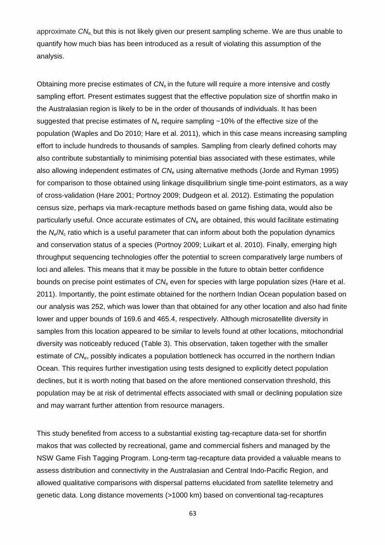
63
approximate CNe, but this is not likely given our present sampling scheme. We are thus unable to
quantify how much bias has been introduced as a result of violating this assumption of the
analysis.
Obtaining more precise estimates of CNe in the future will require a more intensive and costly
sampling effort. Present estimates suggest that the effective population size of shortfin mako in
the Australasian region is likely to be in the order of thousands of individuals. It has been
suggested that precise estimates of Ne require sampling ~10% of the effective size of the
population (Waples and Do 2010; Hare et al. 2011), which in this case means increasing sampling
effort to include hundreds to thousands of samples. Sampling from clearly defined cohorts may
also contribute substantially to minimising potential bias associated with these estimates, while
also allowing independent estimates of CNe using alternative methods (Jorde and Ryman 1995)
for comparison to those obtained using linkage disquilibrium single time-point estimators, as a way
of cross-validation (Hare 2001; Portnoy 2009; Dudgeon et al. 2012). Estimating the population
census size, perhaps via mark-recapture methods based on game fishing data, would also be
particularly useful. Once accurate estimates of CNe are obtained, this would facilitate estimating
the Ne/Nc ratio which is a useful parameter that can inform about both the population dynamics
and conservation status of a species (Portnoy 2009; Luikart et al. 2010). Finally, emerging high
throughput sequencing technologies offer the potential to screen comparatively large numbers of
loci and alleles. This means that it may be possible in the future to obtain better confidence
bounds on precise point estimates of CNe even for species with large population sizes (Hare et al.
2011). Importantly, the point estimate obtained for the northern Indian Ocean population based on
our analysis was 252, which was lower than that obtained for any other location and also had finite
lower and upper bounds of 169.6 and 465.4, respectively. Although microsatellite diversity in
samples from this location appeared to be similar to levels found at other locations, mitochondrial
diversity was noticeably reduced (Table 3). This observation, taken together with the smaller
estimate of CNe, possibly indicates a population bottleneck has occurred in the northern Indian
Ocean. This requires further investigation using tests designed to explicitly detect population
declines, but it is worth noting that based on the afore mentioned conservation threshold, this
population may be at risk of detrimental effects associated with small or declining population size
and may warrant further attention from resource managers.
This study benefited from access to a substantial existing tag-recapture data-set for shortfin
makos that was collected by recreational, game and commercial fishers and managed by the
NSW Game Fish Tagging Program. Long-term tag-recapture data provided a valuable means to
assess distribution and connectivity in the Australasian and Central Indo-Pacific Region, and
allowed qualitative comparisons with dispersal patterns elucidated from satellite telemetry and
genetic data. Long distance movements (>1000 km) based on conventional tag-recaptures

64
comprised 16% of the recaptures and provided further evidence that shortfin mako populations in
the Australasian and Central Indo-Pacific Region utilise oceanic habitats with spatial scales in the
magnitude of 1,000s of km. There was only a single cross-equatorial recapture of a shortfin mako
over the history of the conventional tagging program and when combined with the telemetry data
this suggests that northward movements into equatorial regions (<12° S) may be relatively
uncommon. This is consistent with the results from the genetic data, which also demonstrated
reduced cross-equatorial connectivity.
When considering the geographical isolation of much of Australia’s shelf waters, conventional tag-
recapture data must be viewed cautiously in-terms of potential power to elucidate patterns of
connectivity outside popular mako game fishing regions, given that there are few opportunities for
sharks to be recaptured by recreational fishers in isolated regions of south and southwest
Australia. Outside the eastern recreational/game fishery, the reporting of recaptures relies on
cooperation of commercial line and gillnet fisheries, and long-range charter fleets that are either
not aware of the tagging program, e.g. in High Seas areas beyond the exclusive economic zone
(200 nm), or where shortfin makos may be taken on foreign owned commercial fishing vessels
operating in isolated areas that are potentially less likely to provide tag return data. Movements
from eastern Australia into the Coral Sea, tropical southwest Pacific Ocean (e.g. New Caledonia),
and to and from New Zealand were recorded in the conventional tagging data, which conferred
with the spatial scales of movements determined from the satellite telemetry data and is consistent
with the high degree of genetic connectivity that was observed between locations throughout this
region. Of note, was the low frequency of conventional tag recaptures to the west of Victoria,
however, rather than being reflective of an east west divide we interpret this to be explained by the
isolation of the GAB and southwestern Australia and a lack of access and fishing effort by game
and recreational fishers in areas inhabited by shortfin makos. Neither the satellite telemetry data,
nor the genetic data provided strong evidence of reduced connectivity between the east and west
coasts of Australia.
The spatial distribution of shortfin makos that were satellite tagged in the GAB and Bonney
Upwelling Region extended into northern tropical oceanic waters, south to the Subtropical Front
and in the SW Pacific Ocean and Coral Sea. Fidelity of juvenile shortfin makos was a key feature
between 125 ˚ and 135 ˚E in the Great Australian Bight (Rogers et al. unpublished data), and the
Naturaliste Plateau in the SE Indian Ocean represented a ‘gateway’ where shortfin makos tended
to leave the continental shelf and begin oceanic movements towards seamounts located ~1,260
km NW of Exmouth and ~200 km SSE of Christmas Island. The tropical migrations included the
northern-most movement by a tracked individual (106.35°E, 12.13°S). One shark tagged in the
Bonney Upwelling Region migrated across the central Indian Ocean to an area ~200 km from the
African continent (49.16°E, 40.11°S), representing the western-most movement, while the eastern-

65
most movement was across the Tasman Sea to New Zealand shelf waters (174.69°E, 37.80°S).
This was followed by a northern migration by the same individual of ~2,370 km to tropical waters
to the east of New Caledonia. During the final stages of the preparation of this report, this tag was
still active and this shark inhabited shelf and oceanic waters to the north of New Zealand.
In summary, the telemetry component of this study showed that shortfin makos exhibited several
distinct movement stages. These were either combinations of/or single components of shelf-
oceanic, shelf-residential and highly migratory-oceanic movements. Below we summarise the
spatial scales that defined the movements of individual shortfin makos over different timeframes in
the Australasian and Central Indo-Pacific Region based on minimal distances travelled.
1) Great Australian Bight, Subtropical Front and Indian Ocean (8,776–24,213 km: 262–672 d).
2) Great Australian Bight and western Bass Strait (11,148 km: 249 d).
3) Great Australian Bight, Subtropical Front and NE Indian Ocean (14,693–21,586 km: 320–469 d).
4) Great Australian Bight, Subtropical Front and Coral Sea (10,511–19,964 km: 311–482 d).
5) Eastern Bass Strait, New Zealand and New Caledonia (10,838 km: 318 d, tag still active).
Movements over similar geographical scales have been described for shortfin makos during long-
term telemetry studies in the NE Pacific Ocean, where tropical temperature fronts (at ~ -12–15°S)
align with turning points during return oceanic migrations to shelf waters of the California Current
ecosystem (Block et al. 2011), supporting our findings that this species is among the most mobile
of the large pelagic sharks. This high mobility coupled with their ‘slow’ life history characteristics
and broad vertical habitat preferences (Stevens et al. 2010; Abascal et al. 2011) means that
individuals are likely to interact with a range of fishing gears during the course of their lifespan.
Patterns of high dispersal observed in the long-term conventional tagging and telemetry datasets,
mitochondrial and microsatellite DNA were all in support of the definition of this species as ‘Highly
Migratory’ in the Australasian and Central Indo-Pacific Region and further indicated there was high
spatial connectivity of populations of shortfin mako.

66
Conclusions
In summary, based on the 36 year conventional game fish tagging data-set, a 7-year satellite
tracking dataset, and microsatellite and mitochondrial DNA analyses from 365 samples collected
in six key regions, the most appropriate scale at which to manage the population fished in
Australian State and Commonwealth waters are the boundaries of the Australian and Central Indo
Pacific Region (New Zealand – south west Pacific – Australasian/Indo Pacific Region). This will
need to be refined as further satellite tracking data are collected, and as further genetic data are
collected from the north and south east Pacific Ocean, and southern Indian Ocean.
To summarise the findings of this study for management purposes, we created a ‘conceptual
connectivity plot’ that demonstrates a broad spatial overview and comparison of the scales of
connectivity highlighted by each of the four data sets (Fig. 20). Importantly, while differences
between hemispheres were not detectable in the microsatellite data, mitochondrial DNA, telemetry
and conventional tagging data all indicated there was minimal connectivity at that geographic
scale. Connectivity between the Australian region and neighbouring South African waters via the
Indian Ocean is more complicated to interpret. Despite some evidence of cross Indian Ocean
linkages, the exact tests of population differentiation based on mitochondrial DNA suggested that
connectivity may be reduced (Table 4).
No individuals were tracked from coast to coast across the entire Indian Ocean using satellite
telemetry, however a single individual tagged in the Bonney Upwelling Region off southern
Australia was recorded as far west as the Crozet Plateau in the Indian Ocean (2000 km east of
South Africa), and mitochondrial ΦST estimates (Table 4) and microsatellite DNA analyses (Table
5) indicated connectivity across this region. There was also a high degree of haplotype sharing
between South Africa and Australasian locations.
It is possible that the combination of the eastward flowing South Indian Current, STF, and east-
west running bathymetric features, including the Naturaliste Plateau, Diamantina Fracture Zone
and Broken Ridge form oceanic migratory pathways that facilitate trans-Indian Ocean linkages
between these populations.
Further investigations into the extent of connectivity between Australian and South African waters
would benefit from tracking information from adult individuals, as well as genetic data from
improved sampling of individuals off Western Australia. Other priorities include identification of
regions in the Australasian and Central Indo-Pacific Region used for nursery, pupping and
parturition, and to improve information on the size of breeding populations.
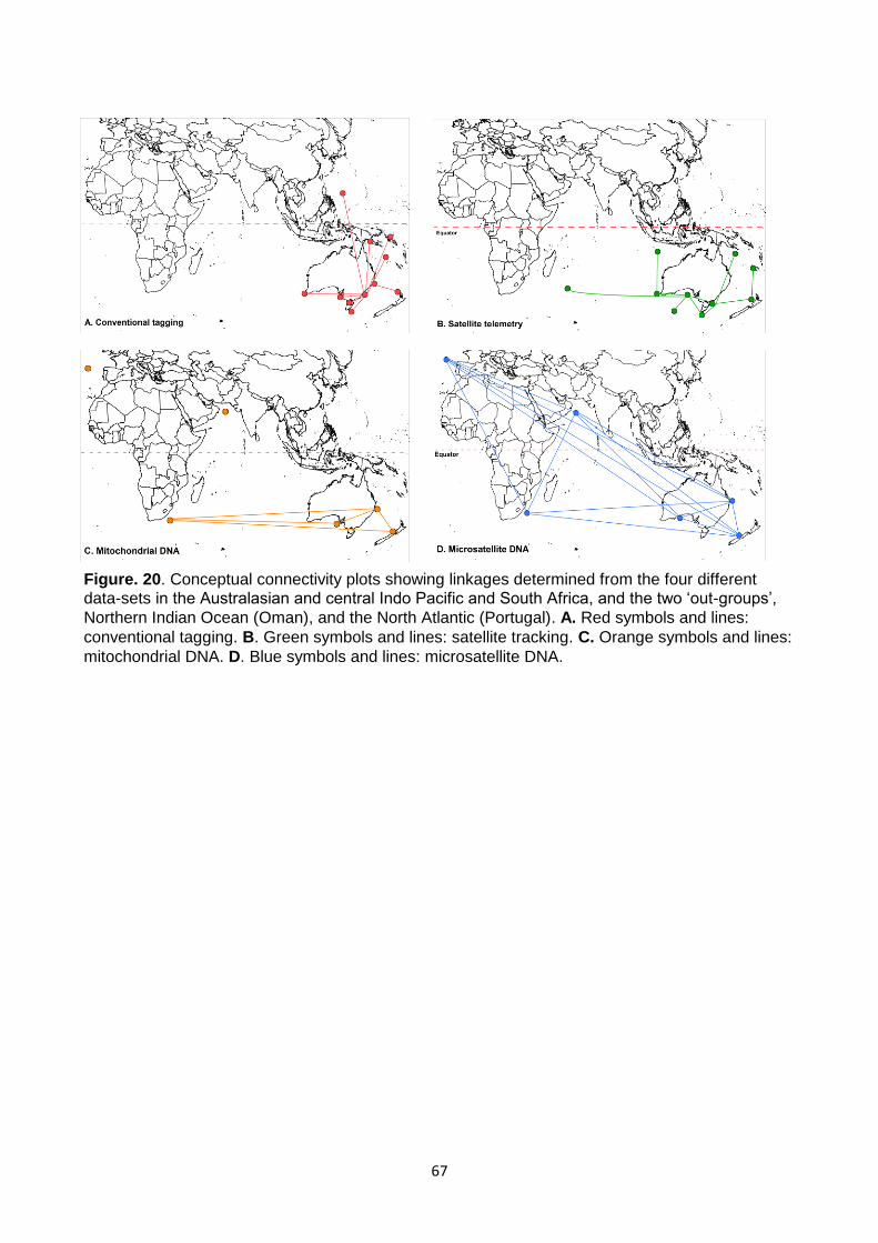
67
Figure. 20. Conceptual connectivity plots showing linkages determined from the four different data-sets in the Australasian and central Indo Pacific and South Africa, and the two ‘out-groups’,
Northern Indian Ocean (Oman), and the North Atlantic (Portugal). A. Red symbols and lines:
conventional tagging. B. Green symbols and lines: satellite tracking. C. Orange symbols and lines:
mitochondrial DNA. D. Blue symbols and lines: microsatellite DNA.

68
Implications
Findings of this study resolve the spatial range, individual movements, stock structure and
effective population size of shortfin mako populations in the Australasian and Central Indo-
Pacific Region, enhancing our ability to inform future risk assessment processes.
This study provides key information that could be incorporated during the IUCN, EBPC,
CITES and CMS assessment processes.
Recommendations
Based on this study, shortfin mako should be managed as an independent, panmictic stock
in Australasia (with New Zealand), but separate from the South African population and the
Northern Hemisphere.
This study highlights that to adequately manage potential impacts on shortfin mako
populations, there is a need for the appropriate RFMOs to consider threatening processes
within the broad spatial distribution of the Australasian and central Indo-Pacific Region.
Findings could be integrated into discussions of appropriate spatial scales for fishery
bycatch regulations of shortfin makos for fisheries managed by Western and Central
Pacific Fishing Commission, Indian Ocean Tuna Commission, and International
Commission for the Conservation of Atlantic Tunas, and Australian State and
Commonwealth fisheries management authorities.
The estimate of effective population size for shortfin makos in the Australasian region is in
the order of thousands of individuals. The lower CI bound (831) of the point estimate of
effective population size of 2,551 is a suitable basal point for discussions pertaining to the
status of the Australasian population with the aim of avoiding declines from this level.
Further efforts should be made to improve the precision of these estimates via more
intensive sampling effort.
Ecological risk assessments undertaken by Western and Central Pacific Fishing
Commission, Indian Ocean Tuna Commission, and International Commission for the
Conservation of Atlantic Tunas have identified the shortfin mako to be among the most
vulnerable shark species to pelagic long-line fisheries in the Indian, western and central
Pacific Oceans (Commission for the Conservation of Southern Bluefin Tuna’s, CCSBT
Working Group, 2013). The CCSBT Ecologically Related Species Working Group
(ERSWG) could integrate the new information on movement and stock structure as part of
ecological risk assessment processes to improve and mitigate ecological impacts of fishing
on the shortfin mako population in the Australasian and central Indo-Pacific Region.

69
Further Development
This project, along with the findings of the workshop to synthesise available data on mako and
porbeagle sharks in Australasian waters (Bruce 2014) together form important basal information
required to further develop regional-scale management policies for these pelagic sharks in the
future. To feed into this process, further spatially explicit risk assessment analyses could be
conducted using the data-streams generated during this project. This could include the
assessment of cumulative impacts of multiple processes on the critical habitats of these pelagic
shark species.
In summary, further development of this research should also seek to:
Better understand the patterns of growth dynamics of shortfin makos in relation to recently
resolved migratory behaviours in the Australasian and Central Indo-Pacific Region.
Resolve sex-biased dispersal hypotheses.
Improve satellite tracking data-sets off eastern Australia with a focus on mature-sized
sharks.
Identify regions in the Australasian and Central Indo-Pacific Region used by shortfin makos
for nursery, pupping and parturition processes.
Improve the precision of preliminary estimates of the order of magnitude of breeding
population sizes provided in this report.
During this project we established a collaboration with researchers at the NOAA Southwest
Fisheries Science Centre, California USA, that are currently generating a DNA data set (both
mitochondrial and microsatellite) for shortfin mako sampled from the northern and southeastern
Pacific regions. We have taken measures to ensure that their emerging data sets are entirely
comparable with our own, via the exchange of reference individuals and by targeting an identical
suite of genetic markers. The aim is to combine these data sets to obtain a global perspective of
genetic structure in this highly mobile species. This will also allow us to assess the degree of
connectivity between Australasian and neighbouring Southern Hemisphere populations, which we
were unable to sample as a part of this study.

70
Extension and Adoption
Findings of this study represent important facets of the scientific information required to
develop Australian Commonwealth Government Environment Department Threatened
Species Recovery Plans.
Findings of this study will be delivered in verbal presentations and in publication formats at
the next available forum of the relevant RFMOs, and sent to the Executive Officers and
relevant representatives of each pelagic fishery.
Information will be made available to the Australian Fisheries Management Authority,
Western and Central Pacific Fishing Commission, Indian Ocean Tuna Commission,
International Commission for the Conservation of Atlantic Tunas, and Australian State
management authorities for incorporation during fisheries ecological/bycatch risk and stock
assessments processes at regional levels.
Findings will be presented at international conferences and made available in the
Australasian and central Indo-Pacific region on Government websites, including those of the
FRDC and SARDI Aquatic Sciences.

71
References
Abascal, F. J., Quintans, M., Ramos-Cartelle, A., and Mejuto, J. (2011). Movements and
environmental preferences of the shortfin mako, Isurus oxyrinchus, in the southeastern
Pacific Ocean. Marine Biology 158, 1175–1184.
Ahonen, H., Harcourt, R.G., and Stow, A. J. (2009). Nuclear and mitochondrial DNA reveals
isolation of imperilled grey nurse shark populations (Carcharias taurus). Molecular
Ecology 18, 4409–4421.
Amante, C., and Eakins, B. W. (2009). ETOPO1 1 Arc-Minute Global Relief Model: Procedures,
Data Sources and Analysis. NOAA Technical Memorandum NESDIS NGDC-24, 19 pp.
Avise, J. C. (2004). Molecular Markers, Natural History and Evolution 2nd Edition. Sunderland,
Massachusetts, Sinauer Associates, Inc.
Bandelt, H. J, Forster, P., and Rohl, A. (1999). Median-joining networks for inferring intraspecific
phylogenies. Molecular Biology and Evolution 16, 37–48.
Banks, S. C., and Peakall, R. (2012). Genetic spatial autocorrelation can readily detect sex-biased
dispersal. Molecular Ecology 21, 2092–2105.
Baum, J. and Worm, B. (2009). Cascading top-down effects of changing oceanic predator
abundances. Journal of Animal Ecology 78, 699–714.
Benavides, M. T., Feldheim, K. A., Duffy, C. A., Wintner S., Braccini, J. M., Boomer J., Huveneers
C., et al. (2011). Phylogeography of the copper shark (Carcharhinus brachyurus) in the
southern hemisphere: implications for the conservation of a coastal apex predator. Marine
and Freshwater Research 62(7), 861–869.
Bird, C., Karl, S., Smouse, P., and Toonen, R. 2011. Detecting and measuring genetic
differentiation. In Crustacean Issues 19 Phylogeography and Population Genetics in
Crustacea. Edited by C. Held, S. Koenemann and C. Schubart. CRC Press. pp. 31-55.
Block, B. A., Jonsen, I. D., Jorgensen, S. J., Winship, A. J., Shaffer, S. A., Bograd, S. J., Hazen,
E. L., Foley, D. G., Breed, G. A., Harrison, A.-L., Ganong, J. E., Swithenbank, A. ,
Castleton, M., Dewar, H., Mate, B. R., Shillinger, G. L., Schaefer, K. M., Benson, S. R.,
Weise, M. J., Henry, R. W., and Costa, D. P. (2011). Tracking apex marine predator
movements in a dynamic ocean. Nature 475 (7354), 86–90.
Blower, D. C., Pandolfi, J. M., Bruce, B. D., Gomez-Cabrera, M., and Ovenden, J. R. (2012).
Population genetics of Australian white sharks reveals fine-scale spatial structure,

72
transoceanic dispersal events and low effective population sizes. Marine Ecology
Progress Series 455, 229–244.
Bonfil, R., Meÿer, M., Scholl, M. C., and Johnson, R., et al. (2005). Transoceanic migration, spatial
dynamics and population linkages of white sharks. Science 310, 100–103.
Bruce, B. D., Stevens, J. D., and Malcolm, H. (2006). Movements and swimming behaviour of
white sharks (Carcharodon carcharias) in Australian waters. Marine Biology 150, 161–
172.
Bruce B. D. (2014) Shark Futures: A synthesis of available data on mako and porbeagle sharks in
Australasian waters - Current status and future directions. Final Report to the Fisheries
Research and Development Corporation - FRDC 2011/045. CSIRO Marine &
Atmospheric Research Hobart Tasmania. 159 pp.
Castro, A. L. F., Stewart, B. S., Wilson, S.G., Hueter, R. E., Meekan, M. G., Motta, P. J., Bowen,
B. W., et al. (2007). Population genetic structure of the Earth's largest fish, the whale
shark (Rhincodon typus). Molecular Ecology 16, 5183–5192.
Chabot C. L., and Allen L. G. (2009). Global population structure of the tope (Galeorhinus galeus)
inferred by mitochondrial control region sequence data. Molecular Ecology 18, 545–552.
Chapman, D. D., Simpfendorfer, C. A., Wiley, T. R., Poulakis, G. R., Curtis, C., Tringali, M.,
Carlson, J. K., et al. (2011). Genetic diversity despite population collapse in a critically
endangered marine fish: the smalltooth sawfish (Pristis pectinata). Journal of Heredity
102, 643–652.
Chesser, R. K., and Baker, R. J. (1996). Effective sizes and dynamics of uniparentally and
diparentally inherited genes. Genetics 144, 1225–1235.
Cockerham, C. (1973). Analysis of gene frequencies. Genetics 74, 679–700.
Compagno, L., M. Dando, et al. (2005). Sharks of the World, Princeton University Press.
Daly-Engel Toby, S., Seraphin Kanesa, D., Holland, K. N., Coffey, J. P., Nance, H. A., Toonen, R.
J., and Bowen, B. W. (2012). Global phylogeography with mixed-marker analysis reveals
male-mediated dispersal in the endangered scalloped hammerhead shark (Sphyrna
lewini). PLoS ONE 7(1), e29986.
Dingle, H. and Drake, V. A. (2007). What Is Migration? Bioscience 57(2), 113–121.
Do, C, Waples, R. S., Peel, D., Macbeth, G. M., Tillett, B. J., and Ovenden, J. R. (2014).
NeEstimator V2: re- implementation of software for the estimation of contemporary

73
effective population size (Ne) from genetic data. Molecular Ecology Resources 14, 209–
214.
Dudgeon, C. L., Blower, D. C., Broderick, D., Giles, J. L., Holmes, B. J., Kashiwagi T, Krück NC ,
et al. (2012). A review of the application of molecular genetics for fisheries management
and conservation of sharks and rays. Journal of Fish Biology 80, 1789–1843.
Dudgeon, C. L., Broderick, D., and Ovenden, J. R. (2008). IUCN classification zones concord with,
but underestimate, the population genetic structure of the zebra shark Stegostoma
fasciatum in the Indo-West Pacific. Molecular Ecology 18, 248–261.
Dulvy, N. K., Baum, J. K., Clarke, S. C., Compagno, L. J. V., Corte´s, E., Domingo, A., Fordham,
S., Fowler, S. L., Francis, M. P., Gibson, C., Martı´nez, J., Musick, J. A., Soldo, A.,
Stevens, J. D., and Valenti, S. (2008). You can swim but you can’t hide: the global status
and conservation of oceanic pelagic sharks and rays. Aquatic Conservation: Marine &
Freshwater Ecosystems 18, 459–482. doi:10.1002/AQC.975.
Duncan, K. M., Martin, A. P., Bowen, B. W., and De Couet, H. G. (2006). Global phylogeography
of the scalloped hammerhead shark (Sphyrna lewini). Molecular Ecology 15, 2239–2251.
Earl, D. A., and vonHoldt, B. M. (2012). STRUCTURE HARVESTER: a website and program for
visualizing STRUCTURE output and implementing the Evanno method. Conservation
Genetics Resources 4, 359–361.
Evanno, G, Regnaut, S., and Goudet, J. (2005). Detecting the number of clusters of individuals
using the software STRUCTURE: a simulation study. Molecular Ecology14, 2611–2620.
Excoffier, L., and Lischer, H. E. L., (2010). Arlequin suite Ver 3.5: a new series of programs to
perform population genetics analyses under Linux and Windows. Molecular Ecology
Resources 10, 564−567.
Falush, D., Stephens, M., and Pritchard, J. K. (2003). Inference of population structure using
multilocus genotype data: linked loci and correlated allele frequencies. Genetics 164,
1567–1587.
Favre, L., Balloux, F., Goudet, J., and Perrin, N. (1997). Female-biased dispersal in the
monogamous mammal Crocidura russula: evidence from field data and microsatellite
patterns. Proceedings of the Royal Society of London Series B 264, 127–132.
Ferretti, F., Worm, B., Britten, G. L., Heithaus, M. R., and Lotze, H. K. (2010). Patterns and
ecosystem consequences of shark declines in the ocean. Ecology Letters 13, 1055–1071.

74
Francis, M., Griggs, L. H., and Baird, S. J. (2001). Pelagic shark bycatch in the New Zealand tuna
longline fishery. Marine and Freshwater Research 52, 165–178.
Francis, M. P., and Duffy, C. (2005). Length at maturity in three pelagic sharks (Lamna nasus,
Isurus oxyrinchus, and Prionace glauca) from New Zealand. Fisheries Bulletin 103, 489–
500.
Francis, M. P. (2013). Commercial catch composition of highly migratory elasmobranchs. New
Zealand Fisheries Assessment Report 2013/68. ISBN 1179-5352. 79 pp.
Frankham, R., Ballou, J. D., and Briscoe D. A. (2010). Introduction to Conservation Genetics.
Cambridge, Cambridge University Press.
GeoScience Australia 2009. http://www.ga.gov.au/
Goudet, J., Perrin, N., and Waser, P. (2002). Tests for sex biased dispersal using genetic
markers. Molecular Ecology 11, 1103–1114.
Goudet, J. (2001). FSTAT, a program to estimate and test gene diversities and fixation indices
(version 2.9.3). http://www.unil/ch/izea/softwares/fstat.html.
Graves, J. E. (1998). Molecular insights into the population structures of cosmopolitan marine
fishes. The Journal of Heredity 89, 427–437.
Greenwood, P. J. (1980). Mating systems, philopatry and dispersal in birds and mammals. Animal
Behaviour 28, 1140–1162.
Hare, M. P. (2001). Prospects for nuclear gene phylogeography. Trends in Ecology and Evolution
16, 700–706.
Hare, M. P., Nunney, L., Schwartz, M. K., Ruzzante, D. E., Burford, M., Waples, R. S., Ruegg, K.,
et al. (2011). Understanding and estimating effective population size for practical
application in marine species management. Conservation Biology 25, 438 –449.
Heist, E. J., and Musick, J. A., et al. (1996). Genetic population structure of the shortfin mako
(Isurus oxyrinchus) inferred from restriction fragment length polymorphism analysis of
mitochondrial DNA. Canadian Journal of Fisheries and Aquatic Sciences 53, 583–588.
Heithaus, M., and Frid, A., et al. (2008). Predicting ecological consequences of marine top
predator declines. Trends in Ecology & Evolution 23, 202–210.
Hill, W. G. (1981). Estimation of effective population size from data on linkage disequilibrium.
Genetical Research 38, 209– 216.

75
Hoelzel, A. R., Shivji, M., Magnussen, J., and Francis, M.P. (2006). Low worldwide genetic
diversity in the basking shark (Cetorhinus maximus). Biology Letters 2, 639–642.
Holdsworth, J. and Saul, P. (2010). New Zealand billfish and gamefish tagging, 2008–09,
Bluewater Marine Research, 34 pp.
Holts, D. (1988). Review of U.S. west coast commercial shark fisheries. Marine Fisheries Review
50, 1–8.
Holts, D. and Bedford, D. (1993). Horizontal and vertical movements of the shortfin mako shark
Isurus oxyrinchus, in the southern California Bight. Australian Journal of Marine and
Freshwater Research 44, 901–909.
Hubisz, M., Falush, D., Stephens, M., and Pritchard, J. K. (2009). Inferring weak population
structure with the assistance of sample group information. Molecular Ecology Resources
9, 1322–1332.
Hueter RE (1998). Philopatry, natal homing and localized stock depletion in sharks. Shark News
12, 1–2.
Jakobsson, M., and Rosenberg, N. A. (2007). CLUMPP: a cluster matching and permutation
program for dealing with label switching and multimodality in analysis of population
structure. Bioinformatics 23, 1801–1806.
Johnson, D., London, J., Lea, M. -A., and Durban, J. (2008). Continuous-time correlated random
walk model for animal telemetry data. Ecology 89(5), 1208–1215.
Jorde, P. E., and Ryman, N. (1995). Temporal allele frequency change and estimation of effective
size in populations with overlapping generations. Genetics 139, 1077–1090.
Jorgensen, S. J., Reeb, C. A., et al. (2010). Philopatry and migration of Pacific white sharks.
Proceedings of the Royal Society B: Biological Sciences 277(1682), 679–688.
Jukes, T. H, and Cantor CR (1969). Evolution of protein molecules. Mammalian protein
metabolism H. Munro. New York Academic Press. 21–132.
Kacev, D. (in prep). The development of novel microsatellite loci for shortfin mako sharks, Isurus
oxyrinchus (order Lamniformes).
Keeney D., Heupel, R., Hueter, R., and Heist, E. (2003). Genetic heterogeneity among blacktip
shark, Carcharhinus limbatus, continental nurseries along the U.S. Atlantic and Gulf of
Mexico. Marine Biology 143, 1039–1046.
76
Keeney, D., Heupel, R., Hueter, R., and Heist E. (2005). Microsatellite and mitochondrial DNA
analyses of the genetic structure of blacktip shark (Carcharhinus limbatus) nurseries in
the northwestern Atlantic, Gulf of Mexico, and Caribbean Sea. Molecular Ecology 14,
1911–1923.
Keeney, D. B., and Heist, E.J. (2006). Worldwide phylogeography of the blacktip shark
(Carcharhinus limbatus) inferred from mitochondrial DNA reveals isolation of western
Atlantic populations coupled with recent Pacific dispersal. Molecular Ecology 15, 3669–
3679.
Klimley, A. P., Beavers, S. C., et al. (2002). Movements and swimming behavior of three species
of sharks in La Jolla Canyon, California. Environmental Biology of Fishes 63, 117–135.
Kohler, N., Turner, P., et al. (2002). Tag and recapture data for three pelagic shark species: blue
shark (Prionace glauca), shortfin mako (Isurus oxyrinchus), and porbeagle (Lamna
nasus) in the North Atlantic Ocean. Collective Volume of Scientific Papers ICCAT 54,
1231–1260.
Loefer, J., Sedberry, G. et al. (2005). Vertical movements of a shortfin mako in the western North
Atlantic as determined by pop-up satellite tagging. Southeastern Naturalist 4, 237–246.
Luikart, G., Ryman, N., Tallmon, D. A., Schwartz, M. K., and Allendorf, F. W. (2010). Estimation of
census and effective population sizes: the increasing usefulness of DNA-based
approaches. Conservation Genetics 11, 355–373.
Luikart, G., Sherwin, W. B., Steele, B. M. and Allendorf, F. W. (1998). (1998). Usefulness of
molecular markers for detecting population bottlenecks via monitoring genetic change.
Molecular Ecology 7, 963–974.
Meirmans, P. G., and Hedrick, P. W. (2011). Assessing population structure: FST and related
measures. Molecular Ecology Resources 11, 5–18.
Michaud A, Hyde J. R., Kohin, S., and Vetter, R. (2011). Mitochondrial DNA sequence data
reveals barriers to dispersal in the highly migratory shortfin mako shark (Isurus
oxyrinchus). In: Report of the Shark Working Group Workshop. Annex 4. International
Scientific Committee for Tuna and Tuna-like Species in the North Pacific Ocean. 38 pp.
Mills, L. S, and Allendorf, F. W. (1996). The one-migrant-per-generation rule in conservation and
management. Conservation Biology 10, 1509−1518.
Mollet, H. F., Cliff, G., Harold, L. Pratt Jr., and Stevens, J. D. (2000). Reproductive biology of the
female shortfin mako, Isurus oxyrinchus Rafinesque, 1810, with comments on the
embryonic development of lamnoids. Fisheries Bulletin 98, 299–318.

77
Mossman, C. A, and Waser, P. M. (1999). Genetic detection of sex-biased dispersal. Molecular
Ecology Notes 8, 1063–1067.
Mucientes, G. R., Queiroz, N., Sousa, L. L., Tarroso, P., and Sims, D. W. (2009). Sexual
segregation of pelagic sharks and the potential threat from fisheries. Biology Letters 5,
156–159.
Musyl, M. K., Domeier, M. L., Nasby-Lucas, N., Brill, R. W., McNaughton, L. M., Swimmer, J. Y.,
Lutcavage, M. S., Wilson, S. G., Galuardi, B., and Liddle, J. B. (2011). Performance of
pop-up satellite archival tags. Marine Ecology Progress Series. 433, 1–28.
Nams, V. O. (2006). Detecting oriented movement of animals. Animal Behaviour 72, 1197–1203.
Nance, H. A., Klimley, P., Galvan-Magana, F., Martınez-Ortiz, J., and Marko, P. B. (2011).
Demographic Processes Underlying Subtle Patterns of Population Structure in the
Scalloped Hammerhead Shark, Sphyrna lewini. PLoS ONE 6, e21459.
Naylor, G. J. P., Caira, J. N., Jensen, K., Rosana, K. M., White, W. T., and Last, P. R. (2012). A
DNA sequence-based approach to the identification of shark and ray species and its
implications for global elasmobranch diversity and parasitology. Bulletin American
Museum Natural History 367, 1–262.
Nei, M. (1987). Molecular Evolutionary Genetics. New York, Columbia University Press. Pp 512.
Paetkau, D., Calvert, W., Stirling, I., and Strobeck, C. (1995). Microsatellite analysis of population
structure in Canadian polar bears. Molecular Ecology 4, 347–354.
Pardini, A. T., Jones, C. S., Noble, L. R., Kreiser, B., Malcolm, H., Bruce B. D., Stevens, J. D., et
al. (2001). Sex-biased dispersal of great white sharks. Nature 412, 139–140.
Peakall, R., Ruibal, M., and Lindenmayer, D. B. (2003). Spatial autocorrelation analysis offers new
insights into gene flow in the Australian bush rat, Rattus fuscipes. Evolution 57, 1182–
1195.
Peakall, R., Smouse, P. E., and Huff, D. R. (1995). Evolutionary implications of allozyme and
RAPD variation in diploid populations of Buffalograss Buchloe dactyloides. Molecular
Ecology 4, 135–147.
Peakall, R., and Smouse, P. E. (2012). GenAlEx 6.5: genetic analysis in Excel. Population genetic
software for teaching and research – an update. Bioinformatics 28, 2537–2539.
Piry, S., Alapetite, A., Cornuet, J. M., Paetkau, D., Baudouin, L., and Estoup, A. (2004).
GeneClass2: A software for genetic assignment and first-generation migrant detection.
Journal of Heredity 95, 536–539.
78
Portnoy, D. S., McDowell, J. R., McCandless, C. T., Musick, J. A., and Graves, J. E. (2009).
(2009). Effective size closely approximates the census size in the heavily exploited
western Atlantic population of the sandbar shark, Carcharhinus plumbeus. Conservation
Genetics 10, 1697–1705.
Posada, D. (2008). jModelTest: Phylogenetic Model Averaging. Molecular Biology and Evolution
25, 1253–1256.
Pritchard, J. K., Stephens, M., and Donnelly, P. (2000). Inference of population structure using
multilocus genotype data. Genetics 155, 945–959.
Prugnolle, F., and de Meeus, T. (2002). Inferring sex-biased dispersal from population genetic
tools: a review. Heredity 88, 161–165.
Palumbi, S. R. (2003). Population genetics, demographic connectivity, and the design of marine
reserves. Ecological Applications 13 Supplement, S146–S158.
Raymond, M., and Rousset, F. (1995). Population genetics software for exact tests and
ecumenicism. Journal of Heredity 86, 248–249.
Rice, W. R. (1989). Analyzing tables of statistical tests. Evolution 43, 223–225.
Rogers P. J., Huveneers, C., Page, B., Goldsworthy, S. D., Coyne, M., Lowther, A. D., Mitchell, J.
G., and Seuront, L. (2015). Living on the continental shelf edge: habitat use of juvenile
shortfin makos Isurus oxyrinchus in the Great Australian Bight, southern Australia.
Fisheries Oceanography. 24: 3, 205–218.
Rosenberg, N. A. (2004). Distruct: a program for the graphical display of population structure.
Molecular Ecology Notes 4,137–138.
Ryman, N., and Palm, S. 2006. POWSIM: a computer program for assessing statistical power
when testing for genetic differentiation. Molecular Ecology 6, 600–602.
Schrey, A. and Heist, E. (2002). Microsatellite markers for the shortfin mako and cross-species
amplification in lamniformes. Conservation Genetics 3, 459–461.
Schrey, A. and Heist, E. J. (2003). Microsatellite analysis of population structure in the shortfin
mako (Isurus oxyrinchus). Canadian Journal of Fisheries and Aquatic Sciences 60, 670–
675.
Schuelke, M. (2000). An economic method for the fluorescent labelling of PCR fragments. Nature
Biotechnology 18, 233–234.

79
Schultz, J. K., Feldheim, K. A., Gruber, S. H., Ashley, M. V., McGovern, T. M., and Bowen, B. W.
(2008). Global phylogeography and seascape genetics of the lemon sharks (genus
Negaprion). Molecular Ecology 17, 5336–5348.
Sepulveda, C. A., Kohin, S. et al. (2004). Movement patterns, depth preferences, and stomach
temperatures of free-swimming juvenile mako sharks, Isurus oxyrinchus, in the Southern
California Bight. Marine Biology 145, 191–199.
Smouse, P. E., Peakall, R., and Gonzales, E. (2008). A heterogeneity test for fine-scale genetic
structure. Molecular Ecology 17, 3389–3400.
Smouse, P. E., and Peakall, R. (1999). Spatial autocorrelation analysis of individual multiallele and
multilocus genetic structure. Heredity 82, 561–573.
Spieth, P. T. (1974). Gene flow and genetic differentiation. Genetics 78, 961–965.
Stevens, J. D. (1992). Blue and mako shark by-catch in the Japanese longline fishery off South-
eastern Australia. Australian Journal of Marine and Freshwater Research 43, 227–236.
Stevens, J., R. Bradford, et al. (2010). Satellite tagging of blue sharks (Prionace glauca) and other
pelagic sharks off eastern Australia: depth behaviour, temperature experience and
movements. Marine Biology 157, 575–591.
Sugiura N (1978). Further analysis of the data by Akaike’s information criterion and the finite
corrections. Communication in Statistics - Theory and Methods. A7, 13–26.
Sunnucks, P., and Hales, D. (1996). Numerous transposed sequences of mitochondrial
cytochrome oxidase in aphids of the genus Sitobion (Hemiptera: Aphididae). Molecular
Biology and Evolution 13, 510–523.
Taguchi, M., Kitamura, T., and Yokawa, K. (2011). Genetic population structure of shortfin mako
(Isurus oxyrinchus) inferred from mitochondrial DNA on inter-oceanic scale. National
Research Institute of Far Seas Fisheries, Japan. 11 pp.
Van Oosterhout, C., Hutchinson, W. F., Wills, D. P. M., and Shipley, P. (2004). Micro-checker:
software for identifying and correcting genotyping errors in microsatellite data. Molecular
Ecology Notes 4, 535–538.
Waples RS (1998). Separating the wheat from the chaff — patterns of genetic differentiation in
high gene flow species. Journal of Heredity 89, 438–450.
Waples RS (2006). A bias correction for estimates of effective population size based on linkage
disequilibrium at unlinked gene loci. Conserv. Genet. 7, 167–184.

80
Waples, R. S., and England, P. R. (2011). Estimating contemporary effective population size on
the basis of linkage disequilibrium in the face of migration. Genetics 189, 633−644.
Waples, R. S., and Do, C. (2010). Linkage disequilibrium estimates of contemporary Ne using
highly variable genetic markers: a largely untapped resource for applied conservation and
evolution. Evolutionary Applications 3, 244−262.
Waters, J. M. (2008) Marine biogeographical disjunction in temperate Australia: Historical
landbridge, contemporary currents, or both? Diversity and Distributions 14, 692–700.
Weir BS (1979). Inferences about linkage disequilibrium. Biometrics 35, 235–254.
Weir BS (1996). Genetic Data Analysis. Sunderland, MA., Sinauer.
Wraith, J. and S. Kohin (2010). Cooperative Anglers and NMFS SWFSC Billfish Newsletter.

81
Appendices
Appendix 1. List of researchers and project staff.
Formulation of project: Paul Rogers and Shannon Corrigan.
Management of project (Primary Investigator): Paul Rogers.
Data management: Paul Rogers (Conventional tagging and satellite telemetry), and Shannon Corrigan (Genetics).
Laboratory analyses: Shannon Corrigan (Genetics).
Fieldwork: Paul Rogers (Satellite telemetry and tissue sampling).
Data analyses: Paul Rogers (Conventional tagging and satellite telemetry), Andrew Lowther (Spatial modelling of satellite telemetry data), and Shannon Corrigan (Genetics).
Report preparation: Paul Rogers (Conventional tagging and satellite telemetry), and Shannon Corrigan (Genetics).

82
Appendix 2. Details of conventional game fish tag-recapture events.
Tag #
Release
date Release location
Recapture
date Recapture location
Days at
liberty
Distance
(km)
1 02-Oct-77 Sydney 30-Oct-77 Redhead 28 52
2 16-Oct-77 Sydney Heads 30-May-78 Sussex Inlet 226 167
3 19-Oct-77 The Peak 06-Nov-77 Broken Bay 18 47
4 27-Mar-79 Unknown 29-Jul-79 Morna Point 124 49
5 28-Dec-80 Swansea 25-Apr-82 Swansea 483 2
6 03-Oct-81 Swansea 10-Jan-82 Terrigal 99 379
7 24-Apr-82 Manly 12-Feb-83 Botany Bay 294 26
8 18-Sep-83 Broken Bay 18-Sep-88 Botany Bay 1827 51
9 17-May-85 Shell Harbour 03-Nov-85 Gibber Reef 170 327
10 11-Aug-85 Point Plomer 25-Apr-86 Tutukaka NZ 257 2051
11 01-Sep-85 Point Plomer 13-May-86 Montague Island 254 605
12 19-Oct-85 Port Stephens 21-Feb-88 Wybung Head 855 69
13 31-Mar-86 Port Stephens 27-May-87 Cape Howe 422 630
14 17-Oct-86 Port Stephens 04-Oct-87 Sydney wide 352 56
15 18-Oct-86 Port Stephens 23-May-87 Box Head 217 113
16 06-Sep-87 Port Macquarie 29-Aug-99 Port Hacking 4375 334
17 18-Oct-87 Garie Beach 26-Sep-88 Coogee 344 35
18 02-Oct-88 Port Macquarie 27-Mar-89 Merimbula 176 623
19 02-Oct-88 Port Macquarie 17-Nov-89 The Banks 411 431
20 01-Oct-89 Sydney 24-Oct-89 Kiama 23 158
21 25-Apr-90 Bermagui 12-Jun-91 Solomon Islands 413 3369
22 29-Apr-90 Montague Island 05-Apr-91 Nadgee River 341 133
23 02-Dec-90 Corrimal 08-May-91 Narooma 157 206
24 14-Apr-91 Tura Head 03-Oct-93 Wollongong 903 302
25 08-Sep-91 Port Stephens Heads 15-Jun-94 King Island 1011 1072
26 26-Apr-92 Bermagui 27-Aug-92 Brisbane 7 1228
27 26-Apr-92 Norah Head 03-May-92 Port Hacking 123 90
28 18-Oct-92 Wave Recording Buoy 24-Feb-93 Gabo Island 129 568
29 02-Nov-92 Port Kembla Wide 16-Jan-93 Cape Conran 75 423
30 28-Nov-92 Redhead 01-Sep-93 Coffs Harbour 277 370
31 24-Jan-93 Bermagui 22-May-93 Bermagui 118 2
32 10-Jul-93 Jervis Bay Canyons 25-Aug-94 Ulladulla 411 23
33 10-Jul-93 Jervis Bay Canyons 10-Oct-94 Norah Head 457 223
34 10-Oct-93 Port Macquarie 16-Oct-93 Forster 6 51
35 26-Dec-93 Eve's Ravene 29-Jan-94 Maringo Beach 34 114
36 24-Apr-94 Narooma 01-Oct-95 Norah Head Canyons 525 363
37 17-Sep-94 Bellambi Point 01-Sep-95 New Caledonia 349 1993
38 27-Feb-95 Bermagui 18-Apr-95 Bermagui 50 25
39 09-Mar-95 Bermagui 14-Apr-95 Eden 36 77
40 06-Jun-95 Bermagui 01-Oct-95 Redhead 117 410
41 27-Jul-95 Kurnell 31-Jul-97 Marion Reef 735 1676
42 13-Aug-95 Swansea 26-May-96 Port Hacking 287 120
43 03-Sep-95 Botany Bay 23-May-96 Tuross Canyons 263 261
44 09-Sep-95 Botany Bay 30-Sep-95 Redhead 21 111
45 28-Oct-95 Shoalhaven Bight 13-May-96 Kangaroo Island 198 1102
46 19-Nov-95 Hare Bay 24-Jan-96 Sydney 66 168
47 27-Jan-96 Bermagui 08-Mar-96 Bermagui 41 21
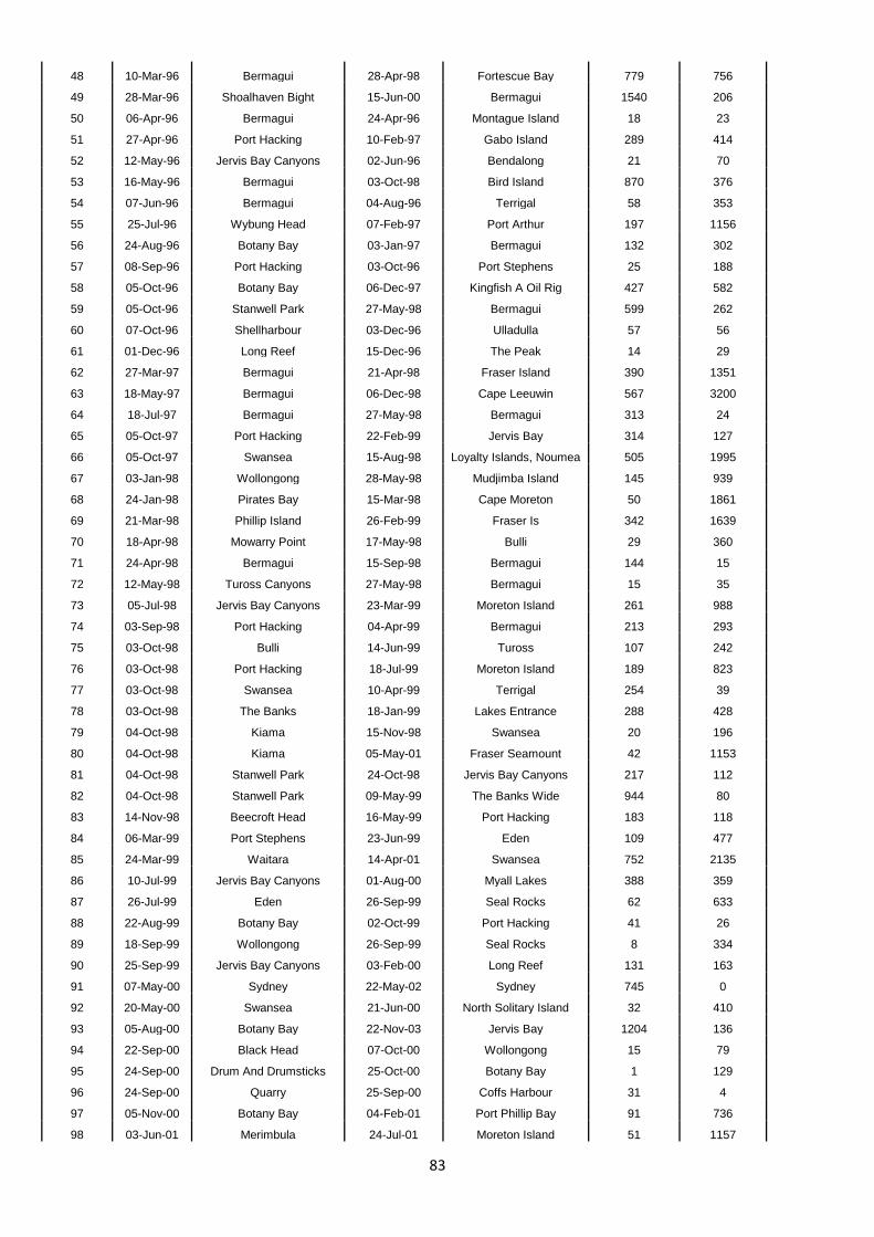
83
48 10-Mar-96 Bermagui 28-Apr-98 Fortescue Bay 779 756
49 28-Mar-96 Shoalhaven Bight 15-Jun-00 Bermagui 1540 206
50 06-Apr-96 Bermagui 24-Apr-96 Montague Island 18 23
51 27-Apr-96 Port Hacking 10-Feb-97 Gabo Island 289 414
52 12-May-96 Jervis Bay Canyons 02-Jun-96 Bendalong 21 70
53 16-May-96 Bermagui 03-Oct-98 Bird Island 870 376
54 07-Jun-96 Bermagui 04-Aug-96 Terrigal 58 353
55 25-Jul-96 Wybung Head 07-Feb-97 Port Arthur 197 1156
56 24-Aug-96 Botany Bay 03-Jan-97 Bermagui 132 302
57 08-Sep-96 Port Hacking 03-Oct-96 Port Stephens 25 188
58 05-Oct-96 Botany Bay 06-Dec-97 Kingfish A Oil Rig 427 582
59 05-Oct-96 Stanwell Park 27-May-98 Bermagui 599 262
60 07-Oct-96 Shellharbour 03-Dec-96 Ulladulla 57 56
61 01-Dec-96 Long Reef 15-Dec-96 The Peak 14 29
62 27-Mar-97 Bermagui 21-Apr-98 Fraser Island 390 1351
63 18-May-97 Bermagui 06-Dec-98 Cape Leeuwin 567 3200
64 18-Jul-97 Bermagui 27-May-98 Bermagui 313 24
65 05-Oct-97 Port Hacking 22-Feb-99 Jervis Bay 314 127
66 05-Oct-97 Swansea 15-Aug-98 Loyalty Islands, Noumea 505 1995
67 03-Jan-98 Wollongong 28-May-98 Mudjimba Island 145 939
68 24-Jan-98 Pirates Bay 15-Mar-98 Cape Moreton 50 1861
69 21-Mar-98 Phillip Island 26-Feb-99 Fraser Is 342 1639
70 18-Apr-98 Mowarry Point 17-May-98 Bulli 29 360
71 24-Apr-98 Bermagui 15-Sep-98 Bermagui 144 15
72 12-May-98 Tuross Canyons 27-May-98 Bermagui 15 35
73 05-Jul-98 Jervis Bay Canyons 23-Mar-99 Moreton Island 261 988
74 03-Sep-98 Port Hacking 04-Apr-99 Bermagui 213 293
75 03-Oct-98 Bulli 14-Jun-99 Tuross 107 242
76 03-Oct-98 Port Hacking 18-Jul-99 Moreton Island 189 823
77 03-Oct-98 Swansea 10-Apr-99 Terrigal 254 39
78 03-Oct-98 The Banks 18-Jan-99 Lakes Entrance 288 428
79 04-Oct-98 Kiama 15-Nov-98 Swansea 20 196
80 04-Oct-98 Kiama 05-May-01 Fraser Seamount 42 1153
81 04-Oct-98 Stanwell Park 24-Oct-98 Jervis Bay Canyons 217 112
82 04-Oct-98 Stanwell Park 09-May-99 The Banks Wide 944 80
83 14-Nov-98 Beecroft Head 16-May-99 Port Hacking 183 118
84 06-Mar-99 Port Stephens 23-Jun-99 Eden 109 477
85 24-Mar-99 Waitara 14-Apr-01 Swansea 752 2135
86 10-Jul-99 Jervis Bay Canyons 01-Aug-00 Myall Lakes 388 359
87 26-Jul-99 Eden 26-Sep-99 Seal Rocks 62 633
88 22-Aug-99 Botany Bay 02-Oct-99 Port Hacking 41 26
89 18-Sep-99 Wollongong 26-Sep-99 Seal Rocks 8 334
90 25-Sep-99 Jervis Bay Canyons 03-Feb-00 Long Reef 131 163
91 07-May-00 Sydney 22-May-02 Sydney 745 0
92 20-May-00 Swansea 21-Jun-00 North Solitary Island 32 410
93 05-Aug-00 Botany Bay 22-Nov-03 Jervis Bay 1204 136
94 22-Sep-00 Black Head 07-Oct-00 Wollongong 15 79
95 24-Sep-00 Drum And Drumsticks 25-Oct-00 Botany Bay 1 129
96 24-Sep-00 Quarry 25-Sep-00 Coffs Harbour 31 4
97 05-Nov-00 Botany Bay 04-Feb-01 Port Phillip Bay 91 736
98 03-Jun-01 Merimbula 24-Jul-01 Moreton Island 51 1157

84
99 29-Sep-01 Botany Bay 17-Apr-05 Eden 1296 363
100 13-Oct-01 Shoalhaven Bight 16-Feb-02 Phillip Island 126 664
101 02-Dec-01 Unknown 25-Apr-02 Fraser Island 144 1010
102 25-Jan-02 Bermagui 22-Jun-02 Clarence Headland 148 838
103 23-Feb-02 Port Stephens 15-Sep-02 Port Stephens 204 25
104 20-Apr-02 Unknown 21-Apr-02 Unknown 1 11
105 03-Nov-02 Bermagui 03-Nov-03 Forster 365 559
106 08-Feb-03 Gerroa 15-Sep-04 Phillipine Sea 585 5940
107 13-Dec-03 Currarong 07-Apr-04 Apollo Bay 116 762
108 20-Dec-03 Bass Point 08-Mar-04 Kilcunda 79 681
109 08-Feb-04 The Entrance 22-Jan-05 Hippolyte Rocks 349 1162
110 28-Feb-04 Port Stephens 19-May-04 Montague Island 81 446
111 20-Mar-04 Broken Bay 16-Apr-04 North Stradbroke Island 27 668
112 20-Mar-04 Cape Schanck 18-Jun-04 Stanwell Park 90 733
113 08-Aug-04 Browns Mountain 08-Aug-04 Browns Mountain 0 0
114 26-Feb-05 Pirates Bay 27-Jul-05 Gold Coast Seaway 151 1740
115 05-Mar-05 Mercury Island 09-Jun-05 Ulladulla 96 2295
116 19-Mar-05 Inverloch 11-Feb-06 Barwon Heads 329 100
117 06-Apr-05 Tabourie Lake 17-Oct-06 Port Moresby 559 2924
118 06-Aug-05 Browns Mountain 07-Jan-06 Cape Otway 154 909
119 06-Aug-05 Browns Mountain 07-Jan-06 Apollo Bay 154 889
120 18-Jan-06 Inverloch 22-Jan-06 San Remo 4 37
121 29-Apr-06 Point Lookout 14-Jun-06 Batemans Bay 46 982
122 07-Nov-06 Coffs Harbour 17-Feb-07 Portsea 102 1190
123 11-Feb-07 Port Stephens 06-May-07 Browns Mountain 84 152
124 17-Feb-07 Kilcunda 19-Jan-08 Cape Schanck 336 22
125 18-Feb-07 Cape Schanck 30-Jul-07 Pacific Ocean 162 2071
126 12-Jan-08 Cape Schanck 27-Apr-08 Cape Schanck 106 1
127 11-Oct-08 Shellharbour Shelf 19-Oct-08 Port Hacking 8 97
128 18-Jan-09 Wilsons Promontory 26-Dec-09 Port Albert 342 44
129 24-Jan-09 St Helens 18-Sep-10 Stanwell Park 602 813
130 22-Feb-09 Cape Schanck 04-Feb-10 Barwon Heads 347 40
131 21-Mar-09 Cody Bank 10-Jan-10 Cape Woolamai 295 33
132 08-Apr-09 Tuross Canyons 10-Apr-09 Kiama Canyons 2 158
133 01-Aug-09 Browns Mountain 02-Aug-09 Browns Mountain 1 111
134 22-Aug-09 Kiama Canyons 22-Aug-09 Greenwell Point 0 15
135 20-Sep-09 Stanwell Park Canyons 08-Jan-10 Flinders Island 110 702
136 20-Sep-09 Stanwell Park Canyons 14-Nov-10 Botany Bay 420 51
137 23-Dec-09 Inverloch 28-Dec-09 Portsea 5 98
138 09-Jan-10 Bass Strait 03-May-10 Tasman Sea 114 1140
139 22-Jan-10 Cape Liptrap 25-Jan-10 Cape Conran 3 262
140 18-Sep-10 Port Hacking 14-Aug-11 Browns Mountain 330 15
141 19-Sep-10 Wollongong 27-Nov-10 Jervis Bay 69 108
142 01-Oct-10 Bermagui 25-Aug-13 Drum Canyons 1059 163
143 05-Dec-10 Shellharbour 08-Feb-11 Lake Tabourie 65 107
144 02-Jan-11 Cape Schanck 15-Jan-11 Lorne 13 75
145 07-Jan-11 Port Macdonnell 19-Mar-11 Cape Liptrap 71 450
146 25-Jan-11 Inverloch 30-Jan-11 Flinders 5 67
147 26-Feb-11 D'Estrees Bay 16-Dec-13 Portland 1024 421
148 27-Feb-11 Inverloch 29-Jan-12 Cape Schanck 336 138
149 17-Sep-11 Wollongong 12-Oct-11 Norah Head 25 161

85
150 25-Nov-11 Jervis Bay 21-Jun-12 Pacific Ocean 209 1717
151 21-Jan-12 Port Welshpool 28-Jan-12 Port Welshpool 7 42
152 04-Aug-12 Browns Mountain 16-Aug-12 Browns Mountain 12 0
153 04-Aug-12 Browns Mountain 25-Aug-12 Browns Mountain 21 2
154 05-Aug-12 Browns Mountain 28-Dec-13 St Helens 510 858
155 09-Sep-12 Browns Mountain 09-Sep-12 Browns Mountain 0 0
156 23-Nov-12 Jervis Bay 11-Jan-13 Cape Schanck 49 666
157 07-Jan-13 Cape Woolamai 20-Jan-13 Cape Woolamai 13 31
158 10-Mar-13 Cape Woolamai 11-Mar-13 Cape Liptrap 1 30

86
Appendix 3. Intellectual Property.

87

88
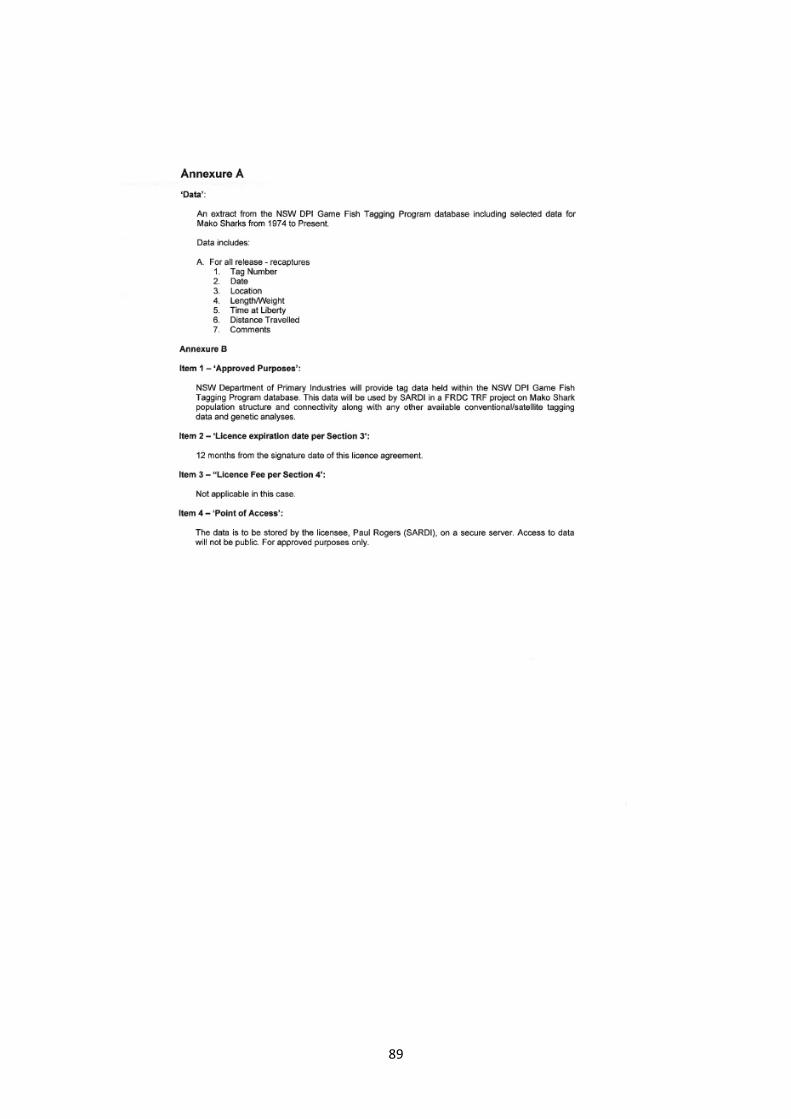
89