Using representative synthetic data to analyze effects of

Using representative synthetic data to analyze effects of filters when processing full

waveform airborne TEM data

Combrinck, M.[1]

_________________________ 1. New Resolution Geophysics, South Africa

OUTLINE

Airborne time domain electromagnetic (ATEM) surveys have reached the stage where full waveform streamed data are recorded and

delivered in addition to traditional survey products. One result of this advance in technology is that the line between the acquisition and

processing phases has become more flexible and many parameters that used to be hardwired in acquisition can now be adapted during the

processing phase. In order to make use of this opportunity the interpreter needs a clear description and understanding of the system specific

corrections required to isolate geological responses as well as the effects of filters and other digital signal enhancement options that are

available.

Validating procedures on a synthetic data set is one way of ensuring that all geological responses falling within similar parameter ranges

would be accurately presented after processing. In this study the effects of three time-series and four spatial filters were analyzed. Streamed

full waveform data were simulated by adding measured high altitude data to synthetic models. The various filters were applied and the

deviations from the true models compared with that of the unfiltered data. The results were evaluated based on whether the filtered results

showed more or less deviation than the unfiltered data from the original noise-free models.

INTRODUCTION

Converting streamed TDEM data into profiles requires a

number of processing steps. These steps vary from

system to system depending on the waveform, geometry

and contractor preferences. Processing steps can be

viewed either as corrections or filters. Corrections are

procedures applied to remove any parts of the measured

data that are systematic, predictable and not due to the

earth’s conductivity response. Filters are used to enhance

the signal to noise ratio of the measured secondary field

based to enhance signal to noise ratios and visual

appearance of data. There are overlaps of course, for

example in the case where applying a correction requires

the use of a filter.

Typical corrections that are applied to recorded data to

provide time gate profiles are:

Subtracting adjacent opposite cycle 50Hz/60Hz

measurements to remove 50Hz/60Hz as well as DC

or very low frequency signal (Macnae et al., 1984)

Removing system response

Normalizing for peak current variations

Gating of streamed data

The application details of these corrections vary from

system to system, based on the configuration central loop

vs towed bird) and waveform (full duty cycle vs partial

duty cycle). Few end users of ATEM data would likely be

in a position to know all different systems intimately enough

to add this level of processing to their interpretation flows.

Filters, on the other hand, can readily be applied by

interpreters to highlight their specific targets of interest and

are largely independent of the system. With the advent of

streamed data recording, the potential is there for

interpreters to get access to data that is much less filtered

than in the past, providing them with more flexibility to

apply filtering routines of their own design.

Most filters are effective in improving precision and making

data more visually appealing, but the question is what the

cost is in terms of accuracy. This paper focuses on a variety

of commonly used filters both in the time and spatial

domains, and quantify what the effects are on the accuracy

of the final results.

FILTER DESCRIPTIONS

The filters that were investigated in this study, are divided

into time series and spatial categories and summarized as

follows.

Time series filters

In cases where streamed data are not recorded these filters

are applied electronically and in the analog domain during

the acquisition phase. Recorded full waveform data enables

us to better evaluate and design these filters.

Despiking

The despiking filter was developed very specifically for

streamed TDEM data processing based on the observed

characteristics of spheric noise (Fig. 1). Spheric events

tend to occur over 200 to 500 samples (6.4 s sampling

interval), and although there is often a single peak that can

be identified, the data are corrupted for up to 500 samples

surrounding the peak. Even if 500 samples are corrupted,

that is less than a quarter of the recorded decay. The

despiking filter is designed to identify these spikes and

only interpolate the affected part of the data stream from

adjacent stations. Filter sensitivity is based on average

noise levels determined from high altitude measurements.

Figure 1: Example of two events of spheric noise. The

top panel shows the transmitter current as reference and

the bottom panel shows the recorded streamed data over

3125 fiducials or 20ms. The first spheric event is

recorded just before the transmitter current is switched on

and the second shortly after the turn-off.

Low Pass Finite Impulse Response (FIR)

FIR filters are applied by convolving a finite number of

coefficients with a time series. The number of coefficients

(filter order plus one) and coefficient values are the

variable parameters. A series of low pass filters between

5 kHz and 15 kHz were designed using the Parks-

McCellan algorithm and applied in Oasis Montaj using a

custom executable file (gx).

Variable Width Averaging (VWA)

The VWA filter was inspired by the concept of variable

width gates used in most, if not all, time domain EM

systems. Time gates (or channels) are chosen to be small

in early times where the signal to noise ratio is high and

the decay changes rapidly with time. They are then

progressively widened with time until many streamed

data samples are averaged to produce a single channel

where the signal to noise ratios are lower and the decay

slope much less than at early times. The VWA filter uses

the same principle and averages values along the times

series using single data samples at positions where the

decay rapidly changes and larger averaging widths where

the decay flattens out. The main difference between this

filter and the normal gating procedure is that there is no

reduction in the number of data points between input and

output, whereas gating would typically reduce 2000 points

to 50 or less. The VWA filter is also applied in Oasis Montaj

using a custom executable file (gx).

Spatial filters

FFT low pass

The FFT low pass filter was applied using Oasis Montaj

software. The filter is based on the method described by

Fraser et al. (1966) and the only variable parameter is the

filter cut-off wavelength.

Stacking (averaging)

The stacking or averaging filter calculates the average of a

specified number of samples with equal weight assigned to

each sample. The only variable parameter is the number of

samples.

Non-linear

The non-linear filter was also applied using Oasis Montaj

software. This filter was first described by Naudy and

Dreyer (1968) and has two variable parameters; the filter

width as well as filter tolerance or noise amplitude.

Polynomial fitting (Savitzky-Golay)

The Savitzky-Golay filter is based on fitting successive sub-

sets of adjacent data points with a polynomial by the method

of linear least squares (Savitzky and Golay, 1964). A stand-

alone algorithm was used to implement this filter with

variable parameters being the filter width and the order of

polynomial to use.

METHODOLOGY

Synthetic data were calculated using 200m x 200m and

400mx400m plates with conductances scaled so that the

decay constants () was 1ms and 5 ms for each of the two

plates. Two sections of data measured at high altitude

during an XciteTM test survey in Ermelo, South Africa were

used as typical examples of AEM noise. One section,

referred to as the “low noise” section was acquired during

optimal survey conditions while the “high noise” section

was acquired during less than ideal conditions with a

thunder storm approaching (Fig. 2).

Maxwell modelling software that was used to calculate the

theoretical plate responses does not allow the calculation of

more than 3000 gates which is typical for streamed data

systems. In order to generate typical model responses

Maxwell was used to calculate the standard off-time

responses for a variety of different plate sizes and depths.

Figure 2: Profiles of “low noise” (bottom) and “high

noise” (top) sections after standard processing.

The conductivities were chosen to give predetermined

decay constant values of 1ms and 5ms which are typical

values that can be detected with 25Hz off-time helicopter

TDEM systems (reference relationship between tau and

geometry). Streamed data responses for these decay

constants were calculated by convolving a measured

system waveform (Combrinck and Wright, 2016) over ten

full waveform cycles with exponential functions of the

form:

𝐹𝜏𝑖(𝑡) = 𝑒−𝑡/𝜏𝑖 ; 𝑖 = 1,5 (1)

These responses are late time approximations and not

accurate for early times, but are sufficient for the purpose

of investigating filter effects in the mid- to late time range

( >170 ms) after turn-off. The full waveform responses

for each decay constant were then scaled to match the

plate modelling software at the overlapping time gates to

account for plate and system geometry and create

streamed data profiles of synthetic data.

Noise sections were added to the model data to give

representative streamed data sets and the minimum

corrections mentioned in the previous section were

applied to each of these. The noise sections were also

processed on their own as separate lines.

In the next phase the different filters (with a range of

parameters) were applied to the modelled data with noise

added, as well as to the noise sections alone.

Standard deviations over 300 points of the noise were

used as estimates of precision for each instance of a filter.

Similarly, standard deviations of the filtered data from the

model data (before any noise were added) over 300 points

were used as estimates for accuracy (Eq. 2).

𝑆𝑡𝑑𝐷𝑒𝑣(𝐹(𝑥)) = √1

𝑛∑(𝑥𝑖 − 𝜇𝑖)2

𝑛

𝑖=1

(2)

where, 𝑛 = 300, 𝜇𝑖 = 𝑚𝑜𝑑𝑒𝑙 𝑣𝑎𝑙𝑢𝑒 𝑤𝑖𝑡ℎ𝑜𝑢𝑡 𝑛𝑜𝑖𝑠𝑒 𝑎𝑑𝑑𝑒𝑑

𝑥𝑖 = 𝑓𝑖𝑙𝑡𝑒𝑟𝑒𝑑 𝑑𝑎𝑡𝑎

RESULTS

The synthetic data combinations were split into 10 lines

labelled as follows:

HN: High noise section, no plate

HN_200_1: 200x200m plate; = 1ms; high noise added




LN: Low noise section, no plate

LN_200_1: 200x200m plate; = 1ms; low noise added




Each of these lines have been processed with the minimum

corrections required to extract 32 gated profiles. The profile

data for these 10 lines are shown in Figure 3. Subsequent

comparisons always used these 10 lines as reference

Standard deviations were calculated over all stations on all

lines, but two locations highlighted on each line were used

to draw comparisons between the various filters.

Combining all the filter variations resulted in 57 sets of

filtered data. Only a few selected examples will be

discussed to illustrate the effects of each filter and the

standard deviations of each results from the original models

will be used as a more comprehensive comparison tool to

include all the data.

Time series filters

Despiking

A profile example of the despiking filter applied to the low

noise case is shown in figure 4. The larger amplitude spikes

have been successfully removed and the effect of this filter

is limited to the spheric affected decays only, unlike a

typical frequency domain filter which affects all the data. In

figure 5 we have the same filter applied to a high noise line.

The only difference is that the filter sensitivity was adjusted

to match the higher standard deviation of the noise. The

despiked profiles are smoother, especially over the plate

anomaly. The general nature of the profiles is still very

noisy and on closer inspection a few samples can be found

where spikes were introduced and worsened the data. This

filter performed better in the low noise case as it is based

on finding single station sharp variations (spherics) in a

more homogeneous background. The high noise case

does not conform to this basic assumption as the spheric

activity dominates the data. As mentioned, this noise

sample was collected as a thunder storm was approaching

and even though the despiking filter is designed to deal

with spheric activity it will underperform if the spheric

interference is continuous or have events that are too close

in time to be treated as individual spikes.

The profile presentation used in figures 4 and 5 are useful

to indicate smoothness of data and provide a qualitative

sense of noise reduction. The next step is to quantify the

filter results in terms of the standard deviation of the

filtered data from the noise-free model data. The standard

deviation is calculated for each channel over 300 points

or 150m. This standard deviation (error) for each filtered

channel is then expressed as a fraction of the error of the

unfiltered data. In this format values smaller than one

indicate that the filter has improved the data and values

larger than one indicate that the error has increased. So,

even though profiles might appear smoother, the filtered

data could be less accurate when compared with the

original models. Figure 6 shows the error fractions of the

two lines from figures 4 and 5, calculated at the stations

indicated with the black dots. The profiles marked with

“b” at the end always correspond to the second station on

the line counting from the left. Although these stations

are indicated as single dots, the errors are calculated for

the 300 points surrounding each one, and the profiles are

therefore representative of more than a single decay.

Figure 6: The error fractions for lines HN_200_1 and

LN_200_1 at two stations on each line.

The low noise line show very little variation from one

except on the first and last three channels of LN_200_1_b.

The reduction in error of the last three channels

corresponds to a late time spike that was successfully

filtered out. The spike is visible on Figure 4 just to the

right of the second marked station (black dot). The

increase in error in the early channels is not immediately

evident and the reason is addressed in a subsequent

paragraph.

The high noise line show improvements on most channels,

but not all. Channels 15 and 23 were made worse in both

example stations. The presentation in figure 6 is useful, but

limited with the number of models that can be compared. In

order to illustrate the effect of the despiking filter on all the

models (2 stations on 10 lines) the average of the error

fraction over the 32 channels are calculated and displayed as

a function of the line and center station (Figure 7).

Figure 7: The average error fractions of the despiking filter

for all model lines and stations.

Apart from LN_200_5b and HN 400_5b it is clear that the

low noise lines are generally slightly improved, and that the

high noise lines are improved on average, even if not for

every channel individually. Closer inspection of

LN_200_5b and HN 400_5b revealed that the anomaly peak

curvatures were so sharp that they were treated as spikes as

well. This also happened on some of the other lines and was

the reason for the first three channels in Figure 6 to have

error fractions more than one. However, on LN_200_5b and

HN 400_5b the majority of channels were picked as spikes

resulting in an average error fraction larger than one.

FIR

Fifteen instances of the FIR filter were tested in total Filters

were designed to have cut-off frequencies of 5, 10 and 15

kHz. In a first run, each of these frequencies were

implemented with 6, 11 and 16 coefficients corresponding

to 5th, 10th and 15th order filters. The results from this first

attempt indicated that the filters using an even number of

points (5th and 15th order) introduced much larger errors

than the 10th order filter for the same cut-off frequencies.

One of the more extreme examples is shown in Figure 8a.

The effect was more pronounced on the low noise data lines

over the anomalies where the signal was strongest. It

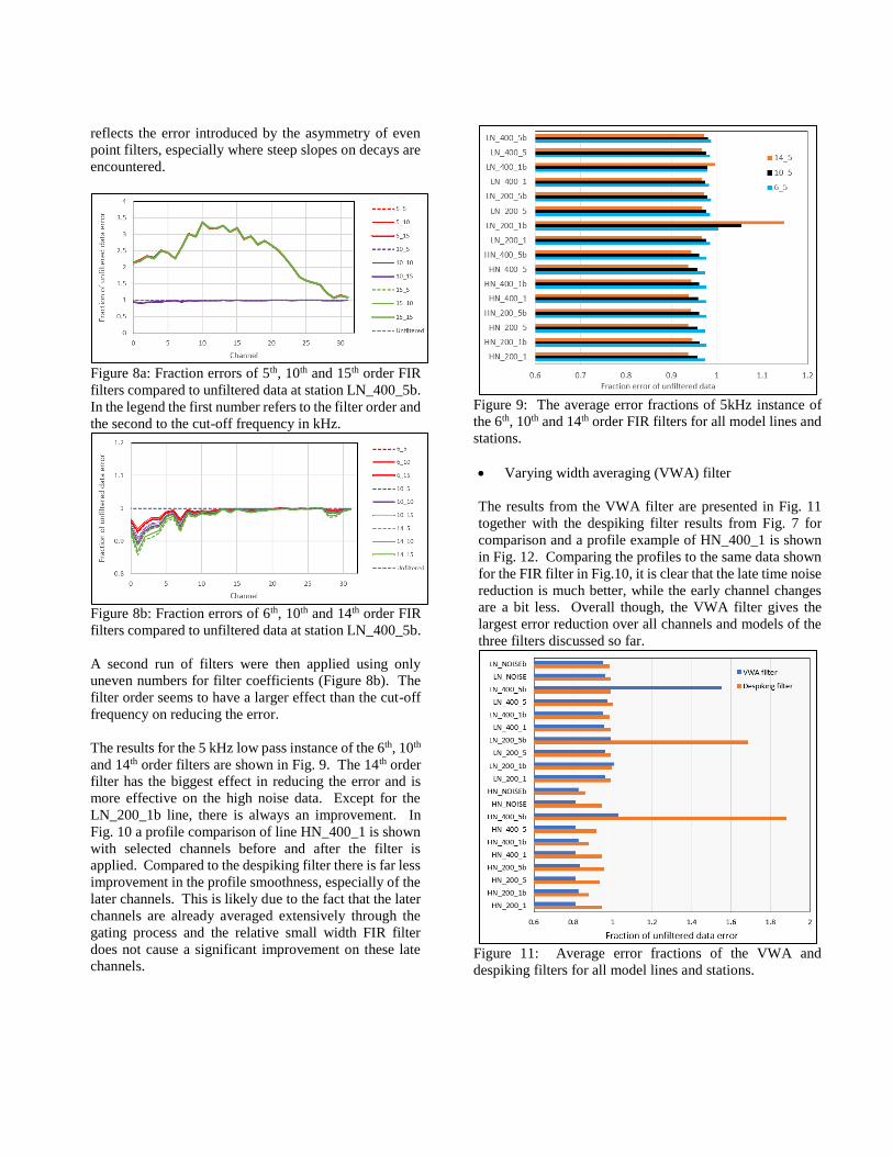
reflects the error introduced by the asymmetry of even

point filters, especially where steep slopes on decays are

encountered.

Figure 8a: Fraction errors of 5th, 10th and 15th order FIR

filters compared to unfiltered data at station LN_400_5b.

In the legend the first number refers to the filter order and

the second to the cut-off frequency in kHz.

Figure 8b: Fraction errors of 6th, 10th and 14th order FIR

filters compared to unfiltered data at station LN_400_5b.

A second run of filters were then applied using only

uneven numbers for filter coefficients (Figure 8b). The

filter order seems to have a larger effect than the cut-off

frequency on reducing the error.

The results for the 5 kHz low pass instance of the 6th, 10th

and 14th order filters are shown in Fig. 9. The 14th order

filter has the biggest effect in reducing the error and is

more effective on the high noise data. Except for the

LN_200_1b line, there is always an improvement. In

Fig. 10 a profile comparison of line HN_400_1 is shown

with selected channels before and after the filter is

applied. Compared to the despiking filter there is far less

improvement in the profile smoothness, especially of the

later channels. This is likely due to the fact that the later

channels are already averaged extensively through the

gating process and the relative small width FIR filter

does not cause a significant improvement on these late

channels.

Figure 9: The average error fractions of 5kHz instance of

the 6th, 10th and 14th order FIR filters for all model lines and

stations.

Varying width averaging (VWA) filter

The results from the VWA filter are presented in Fig. 11

together with the despiking filter results from Fig. 7 for

comparison and a profile example of HN_400_1 is shown

in Fig. 12. Comparing the profiles to the same data shown

for the FIR filter in Fig.10, it is clear that the late time noise

reduction is much better, while the early channel changes

are a bit less. Overall though, the VWA filter gives the

largest error reduction over all channels and models of the

three filters discussed so far.

Figure 11: Average error fractions of the VWA and

despiking filters for all model lines and stations.

Spatial filters

The four spatial filters all have a filter width variable. The

widths for each one were changed from 21 to 201 fiducials

in intervals of twenty. Although the exact effects of the

filter widths are different for the different filters, it is used

as a practical means to draw comparisons between the

four. Figures 13-16 summarize the effects of the spatial

filters on the different data sets.

Figure 13: Average error fractions as a function of low

pass filter width.

Figure 14: Average error fractions as a function of

stacking filter width.

The=5ms conductors show the largest errors on all

filters while the high noise lines with =1ms conductors

benefit the most from filtering.

Figure 15: Average error fractions as a function of non-

linear filter width.

Figure 16: Average error fractions as a function of

Savitzky-Golay filter width.

In most cases an initial reduction in error is observed for

short filter widths and then followed by a steady increase in

error with increasing filter width. The filter width where

this change occurs and also the rate at which the errors

increase is dependent on the filter type. In figures 17 and 18

some results are regrouped to better visualize the effects of

the different filters.

In figure 17 all the low noise (LN) lines are grouped

together. All these models show an increase in error with

filtering but the Savitzky-Golay filter causes the smallest

error increase, closely followed by the low pass filter.

Figure 17: Average error fractions for the low noise

models.

In figure 18 the high noise (HN) results are shown. With

this group we see an initial error reduction for all filters.

The low pass and Savitzky-Golay filters can be applied

with filter widths up to 80 and 60 fids respectively before

the errors start increasing.

Figure 18: Average error fractions for the high noise

models.

Profile comparisons of these filters are shown in figures

19 and 20 for filter widths of 101 fids. The two lines that

are shown are the ones that benefited the most

(HN_400_1) and the least (LN_400_5) from the spatial

filters. It is interesting to note that while the non-linear

filter gave the best results on HN_400_1 it also gave the

worst results by far on LN_400_5.

CONCLUSIONS

Recording of streamed data in modern ATEM systems

allow corrections and filters that were traditionally

applied during acquisition to now be implemented in the

processing phase. As advanced filtering now becomes an

optional post-acquisition procedure it is crucial for

processors and interpreters to understand the effects of these

filters on data.

A simple yet effective method was used to calculate errors

and evaluate the effects of various filters on streamed data

sets. Even though the number of filters and models included

in this study are by no means representative of all options

and environments it is clear that significant errors can be

introduced if the only aim (and measure of success) is to

provide smooth and visually appealing data. Most filters

will change the input data in some way. Comparing the

results from the spatial filters on high and low noise data

(Figures 17 and 18) illustrates that high noise data can

benefit from filtering but that low noise data do not. Of the

filters examined here the VWA and the Savitsky-Golay

filters showed the most promising results applied to the time

series and spatial data respectively. The VWA filter is

effective because it filters the high noise (late time) data

more than the low noise data (early time). Developing filters

that apply a similar principle in the space domain, based on

data amplitudes and lateral spatial gradients could be

investigated in future.

ACKNOWLEDGEMENTS

Thank you to NRG for use of streamed data samples and

Richard Wright (NRG Engineering Manager) for his

invaluable contributions in designing filters and developing

software for this study.

REFERENCES

Combrinck, M., Wright, R., 2016, “Achieving accurate

interpretation results from full-waveform streamed data

AEM surveys”: ASEG_PESA 2016, Adelaide, Australia,

Expanded Abstracts

Fraser, D.C., Fuller, B.D. and Ward, S.H., 1966. “Some

numerical techniques for application in mining

exploration.”: Geophysics, 31(6), 1066-1077.

Macnae, J.C., Lamontagne, Y., and West, G.F., 1984,

“Noise processing techniques for time-domain EM

systems”: Geophysics 49, 934-948.

Naudy, H., and Dreyer, H., 1968, “Essai de filtrage non-

lineaire appliqué aux profiles aeromagnetiques (Attempt to

apply nonlinear filtering to aeromagnetic profiles)”:

Geophysical Prospecting, 16, 171-178.

T. W. Parks and J. H. McClellan., 1972, “Chebyshev

approximation for nonrecursive digital filters with linear

phase.”: IEEE Trans. on Circuit Theory, 19:189–94.

Savitzky, A., Golay, M.J.E. (1964). “Smoothing and

Differentiation of Data by Simplified Least Squares

Procedures": Analytical Chemistry, 36 (8): 1627–39.

Figure 3a: Profiles of high noise lines. Panel 1: HN - High noise section, no plate. Panel 2: HN_400_5 - 400x400m plate; =

5ms; high noise added. Panel 3: HN_400_1 - 400x400m plate; = 1ms; high noise added. Panel 4: HN_200_5 - 200x200m

plate; = 5ms; high noise added. Panel 5: HN_200_1 - 200x200m plate; = 1ms; high noise added. The black dots indicate

the stations referenced for decay analysis and standard deviation comparisons.

Figure 3b: Profiles of low noise lines. Panel 1: LN - Low noise section, no plate. Panel 2: LN_400_5 - 400x400m plate; =

5ms; low noise added. Panel 3: LN_400_1 - 400x400m plate; = 1ms; low noise added. Panel 4: LN_200_5 - 200x200m plate;

= 5ms; low noise added. Panel 5: LN_200_1 - 200x200m plate; = 1ms; low noise added. The black dots indicate the

stations referenced for decay analysis and standard deviation comparisons.

Figure 4: Low noise example of the despiking filter. A section of the line (LN_200_1) with the 200x200m plate ( = 1ms) and

low noise added is shown in the top panel. The middle panel illustrates the same channels after the despiking filter has been

applied. The bottom panel compare the last channel only of the unfiltered data (black) and the despiked data (red).

Figure 5: High noise example of the despiking filter. A section of the line (HN_200_1) with the 200x200m plate ( = 1ms) and

high noise added is shown in the top panel. The middle panel illustrates the same channels after the despiking filter has been

applied. The bottom panel compares the last channel only of the unfiltered data (black) and the despiked data (red).

EM R

esp

on

se [

pV

/m^4

]; lo

g-lin

sca

le b

ase

10

0

EM R

esp

on

se [

pV

/m^4

]; lo

g-lin

sca

le b

ase

10

0

Figure 10: High noise example of the 5kHz low pass, 14th order FIR filter. A section of the line (HN_400_1) with the 400x400m

plate ( = 1ms) and high noise added is shown in the top panel. The second panel illustrates the same channels after the FIR

filter has been applied. The third panel compares the last channel only of the unfiltered data (black) and the filtered data (red).

The bottom panel shows the third channel of the unfiltered data (black) and the filtered data (red).

EM R

esp

on

se [

pV

/m^4

]; lo

g-lin

sca

le b

ase

10

0

Figure 12: High noise example of the VWA filter. A section of the line (HN_400_1) with the 400x400m plate ( = 1ms) and

high noise added is shown in the top panel. The second panel illustrates the same channels after the VWA filter has been

applied. The third panel compares the last channel only of the unfiltered data (black) and the filtered data (red). The bottom

panel shows the third channel of the unfiltered data (black) and the filtered data (red).

EM R

esp

on

se [

pV

/m^4

]; lo

g-lin

sca

le b

ase

10

0

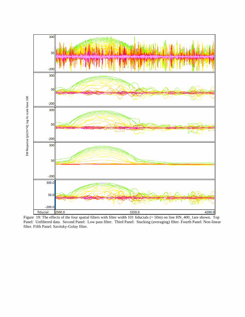
Figure 19: The effects of the four spatial filters with filter width 101 fiducials (= 50m) on line HN_400_1are shown. Top

Panel: Unfiltered data. Second Panel: Low pass filter. Third Panel: Stacking (averaging) filter. Fourth Panel: Non-linear

filter. Fifth Panel: Savitsky-Golay filter.

EM R

esp

on

se [

pV

/m^4

]; lo

g-lin

sca

le b

ase

10

0

Figure 20: The effects of the four spatial filters with filter width 101 fiducials (= 50m) on line LN_400_5 are shown. Top

Panel: Unfiltered data. Second Panel: Low pass filter. Third Panel: Stacking (averaging) filter. Fourth Panel: Non-linear

filter. Fifth Panel: Savitsky-Golay filter.

EM R

esp

on

se [

pV

/m^4

]; lo

g-lin

sca

le b

ase

10

0

Documents

Using representative synthetic data to analyze effects of