Using Regression-based Sensitivity Analysis in Exploratory

http://mi.water.usgs.gov/reports/images/cover_med01_4227.jpg

Using Regression-based Sensitivity Analysis in Exploratory Modeling of Complex Spatial Systems:

An Example of Simulating the Impact of Agricultural Water Withdrawals on Fish Habitat

Glenn O’Neil (Institute of Water Research – Michigan State University)

Arika Ligmann-Zielinska, Ph.D. (Department of Geography – Michigan State University)

AAG Annual Meeting Los Angeles, CA 4/9/2013

AAG Annual Meeting Los Angeles, CA 4/9/2013

Regression-based Sensitivity

Introduction ABM Model Sensitivity Analysis Conclusion

Research Question:

What issues arise in employing regression techniques to evaluate the sensitivity of a complex, agent-based spatial model to its individual parameters?

2

Overview:

- Conceptual agent-based model of fish habitat impacts from agricultural water withdrawals.

- Model sensitivity analysis through OLS regression.

- Issues with count data

- OLS alternative: negative binomial with hurdle



3

Conceptual Model - Farmlands (CLUs) (land owner agents)

- Agricultural Demand Index

- Likelihood of CRP enrollment

- Land use change decisions – withdrawal installations

- Reductions in baseflow1

- Decline in fish sustainability2

CLU boundary

Forest

Grassland / Pasture

Row-crop

Water

Existing withdrawal

Proposed withdrawal 1. Reeves 2008. 2. Zorn, et. al. 2008.



4

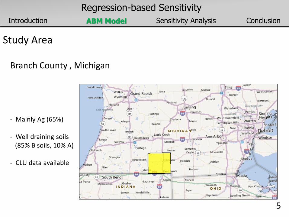
Study Area

Branch County , Michigan

- Mainly Ag (65%) - Well draining soils (85% B soils, 10% A) - CLU data available



5

Fish Habitat Data

M-DNR: - Tolerable baseflow reductions

Sensitive Fish Sustainability

Available GW Depletion (GPM)

107 - 243

244 - 515

516- 1,887

1,888 - 3,140

3,141 - 10,507

Branch County



6

Model Output / Dependent Variable

• Change in fish habitat sustainability over time (Years To Stop) - Reduction in baseflow - Change in stream fish habitat classification

0

2

4

6

8

10

12

14

16

1 2 to 5 6 to 10 11 to 14 15 - 18 19 - 23 > 23

Co

un

t

Years until sensitive fish no longer supported at more than 75% of streams

40 model runs



7

Model Parameter Categories / Regression Independent Vars.

• Crops - area % - prices - price variability

• CRP enrollment - starting enrollment - probability of re-enrollment - contract length

• Land cover change probabilities - Given revenues of $X, probability that a producer would convert Y to Z.

• Decision thresholds - revenue level above which producers will consider increased irrigation, below which they will consider CRP



8

Model Sensitivity Analysis

• Ran the model over 1,400 times with randomly selected parameter values

• Employed OLS regression -DV: Years until 75% of streams no longer support sensitive fish - IVs: model parameters

• Expectations Starting corn prices -

Starting soy prices - Corn area % - Soy area % - Crop price variability ? Soy price variability ?

Corn yield per acre - Soy yield per acre -

Revenue threshold to move land into production + Revenue threshold to move land into conservation - Ratio of market increase to CRP decrease - Starting % enrolled in CRP + CRP contract length + CRP renewal probability + Probability of conversion to pasture + Probability of conversion to forest + Probability of conversion to wetland +



9


• Identified best models through an exhaustive approach - 17 model parameters - max of 7 independent variables at a time - 41,226 regressions - sorted by R2, F-statistic, % of significant terms

• Is this rummaging? - Not trying to explore or discover variable relationships - The model is programmed to have relationships - Trying to identify weights of individual variables

10




• Best OLS model

• Standardized coefficients

ln(Years to stop) = 2.23 – (0.173* corn price) – (0.141*corn price variability) – (0.009*corn yield) – (0.010*soy yield) + (0.002 * land production revenue threshold)

R2 0.35

F-statistic prob. < 0.001

Sig. ind. vars all

Corn price -0.444

Soy yield -0.328

Corn yield -0.303

Land production revenue threshold 0.268

Corn price variability -0.230 11




Further inspection showed a poor fit

Why?

DV is a count, OLS won’t work

0.0 0.5 1.0 1.5

-1.0

-0.5

0.0

0.5

1.0

Fitted values

Re

sid

ua

ls

lm(YearsToStopLog ~ StartingCornPrice + CornPriceChangeSD + CornBushelYield ...

Residuals vs Fitted

792

563

457

Residuals vs. Fitted Values

Res

idu

als

Fitted



12


• Employed a negative binomial regression, with a hurdle component as an alternative3,4. Histogram of runszero$YearsToStop

runszero$YearsToStop

Fre

qu

en

cy

0 20 40 60 80 100

02

00

40

06

00

Years To Stop

Freq

uen

cy

Hurdle component models zero values separately, essentially as a logit model. Remainder modeled with negative binomial regression

• Useful for over-dispersed, skewed data with large zero counts. • Function hurdle() from the pscl R package.

3. cran.r-project.org/web/packages/pscl/vignettes/countreg.pdf 4. http://www.ats.ucla.edu/stat/mplus/dae/nbreg.htm



13


• Best negative binomial hurdle model (sorted by AIC)

• Difficult to standardize coefficients

Years to stop = (count model)

7.72 – (0.731* corn price) – (0.657*corn price variability) – (0.038*corn yield) – (0.047*soy yield) + (0.009 * land production revenue threshold) - ln(θ)

Years to stop = (zero model)

6.76 – (0.352*corn price) – (0.019*corn yield) – (0.020*soy yield) - ln(θ)

Sig. ind. Vars All but θ

AIC 74741



14


• Hurdle coefficient standardization options - z-score ratios

- hierarchical partitioning - Murray and Connor 2009

- R package hier.part

Corn price -0.349

Soy yield -0.298

Corn yield -0.260

Corn price variability -0.229

Land production revenue threshold 0.137

count model

Corn price -0.386

Soy yield -0.309

Corn yield -0.305

zero model



15


Further inspection showed hurdle was still a poor fit

Why?

Still struggling with skewness. Transformation of DV makes it no longer a count.

Residuals vs. Fitted Values

Res

idu

als

Fitted 0 20 40 60 80 100 120

-60

-40

-20

02

04

06

08

0

hurdle45_adjusted$fitted.values

hu

rdle

45

_a

dju

ste

d$

resid

ua

ls



16

• Regression can be utilized to estimate parameter weights in complex spatial model. • Issues arise when the dependent variable is count data - Poisson and negative binomial regression are viable alternatives

for over-dispersed data - hurdle models for large zero counts

• Dependent variable skewness is significant challenge - normally distributed continuous data is preferable - not always feasible for agent-based models based on steps

• The example fish habitat sustainability model was most sensitive to market-based parameters (corn price, price variability, production revenue thresholds).



17

Special Thanks: Dr. Jon Bartholic (Institute of Water Research - Michigan State University) Brad Love (Branch County Conservation District) Robert Pigg (Michigan Department of Agriculture)

References: Reeves, H.W., 2008,STRMDEPL08—An extended version of STRMDEPL with additional analytical solutions to calculate streamflow depletion by nearby pumping wells: U.S. Geological Survey Open-File Report 2008–1166, 22 p. Zorn, T., Seelbach, P., Rutherford, T., Cheng, S., Wiley, M. 2008. “A Regional-scale Habitat Suitability Model to Assess the Effects of Flow Reduction on Fish Assemblages in Michigan Streams.” Michigan Department of Natural Resources, Fisheries Report 2089, Ann Arbor. Murray, K., Connor, M. 2009. “Methods to Quantify Variable Importance: implications for the analysis of noisy ecological data.” Ecology, 90(2): p. 348-355.



18

Documents

Using Regression-based Sensitivity Analysis in Exploratory