Using redundant internal coordinates to optimize equilibrium geometries and transition states

Using Redundant Internal Coordinates to Optimize Equilibrium Geometries and Transition States

CHUNYANG PENG, PHILIPPE Y. AYALA, and H. BERNHARD SCHLEGEL" Department of Chemistry, Wayne State University, Detroit, Michigan 48202

MICHAEL J. FRISCH Lorentzian, lnc., North Haven, Connecticut 06473

Received 17 December 1994; accepted 15 May 1995

ABSTRACT A redundant internal coordinate system for optimizing molecular geometries is constructed from all bonds, all valence angles between bonded atoms, and all dihedral angles between bonded atoms. Redundancies are removed by using the generalized inverse of the G matrix; constraints can be added by using an appropriate projector. For minimizations, redundant internal coordinates provide substantial improvements in optimization efficiency over Cartesian and nonredundant internal coordinates, especially for flexible and polycyclic systems. Transition structure searches are also improved when redundant coordinates are used and when the initial steps are guided by the quadratic synchronous transit approach. 0 1996 by John Wiley & Sons, Inc.

Introduction

eometry optimization is an important aspect G of almost all electronic structure calculations. Most of the optimizations are carried out using some variety of quasi-Newton algorithm employing energies and gradients. Geometry optimization has been reviewed in several articles.'

*Author to whom all correspondence should be addressed.

The efficiency of an optimization depends on a number of factors: (1) the initial geometry, (2) the choice of coordinate system, (3) the initial estimate of the Hessian, (4) the Hessian updating method, and (5) control of the search direction and step size.

As an estimate for the starting geoinetry for optimizing equilibrium structures, standard geometries or structures obtained by molecular mechanics minimization are often good. For transition structures, many quasi-Newton methods need to

Journal of Computational Chemistry, Vol. 17, No. 1, 49-56 (1996) 0 1996 by John Wiley & Sons, Inc. CCC 01 92-8651 196 1 01 0049-08

PENG ET AL.

start fairly close to the quadratic region of the transition state. However, initial estimates for transition structures are more difficult to obtain than for equilibrium structures. Molecular mechanics generally cannot handle transition states involving the making and breaking of bonds. Standard geometries are available for some types of transition states,' but transition state geometries vary much more than equilibrium geometries. Techniques such as synchronous transit? coordinate driving, walking up valleys, and eigenvector following4 may be useful in getting close to the transition structure.

Early work in geometry optimization using electronic structure methods used nonredundant internal coordinates ( eg , the Z matrix internal coordinates used in many molecular orbital programs). Cartesian coordinates were shown to be better for some cyclic molecule^,^ and mixed Cartesian and internal coordinates also had some advantages.6 Cartesian normal modes have also been used successfully.7 However, Pulay8-" demonstrated clearly that redundant internal coordinates are the best choice for minimizing polycyclic molecules. Baker" compared redundant internal to Cartesian coordinates and came to a similar conclusion. In the present work, we adopted a simpler system of redundant internal coordinates (but with more redundancies) than we have used previously to estimate the initial Hessian." We have also extended the use of redundant internal coordinates to transition structure optimization using a synchronous transit guided quasi-Newton method.I3

For the choice of the initial Hessian, Baker5," showed that minimizations with Cartesian and redundant internal coordinates were similar if a good initial estimate of the Hessian is used (i.e., a molecular mechanics Hessian instead of a unit Hessian). In this article we use a simple valence force field that is diagonal in the redundant internal coordinate system, similar to the one used in our earlier work." Proper updating of the Hessian is essential for efficient optimizations; most modern updating algorithms give similar results and therefore will not be discussed here.

Choice of the search direction and control of step size are important in determining the efficiency of the optimization.' Trust radius and eigenvector following4 methods have been shown to be effective. For transition states, it is highly desirable to monitor the direction of the transition vector (i.e., the eigenvector corresponding to the negative eigenvalue). In previous workI3 we found

that the tangent to the linear or quadratic synchronous transit path3 was useful in choosing the uphill search direction for optimizing transition states.

Method

GENERATION OF REDUNDANT INTERNAL COORDINATES

Pulay and co-workers'-'' defined a natural internal coordinate system that is similar to the coordinates used by vibrational spectroscopists. It min- imizes the number of redundancies by using local pseudosymmetry coordinates about each atom and special coordinates for ring deformation, spiro ring fusions, etc. Similar coordinates are used by Baker'' and in T~rboMole.'~ To reduce the number of special cases, we use a simpler set of internal coordinates composed of all bond lengths, valence angles, and dihedral angles. This coordinate set, however, has somewhat greater redundancy than the coordinates used by Pulay, but this does not seem to affect the efficiency of the optimization.

Our redundant internal coordinates set is defined in the following manner. First, the inter- atomic distances are examined to determine which atoms are bonded. Two atoms are considered bonded if their separation is less than 1.3 times the sum of the (single bond) covalent radii of the two atoms. If the molecular system consists of two or more fragments that are not bonded by this crite- rion, then the shortest distance between the fragments is determined; all interfragment distances that are less !ban the smaller of 1.3 times this distance, or 2 A, are designated as bonds. A hydrogen bond is indicated if the XH . - * Y distance (X, Y = N, 0, F, P, S, Cl) is greater than the sum of the covalent radii, less than 0.9 times the sum of the van der Waals radii, and the X-H...Y angle is greater than 90". A bond stretching coordinate is assigned to each regular, interfragment, and hydrogen bond.

A valence angle bend coordinate is assigned for any two atoms bonded to the same third atom (LA-B-C, where A is bonded to B and C is bonded to B). Special attention must be given to linear valence angles. If the A-B-C angle is greater than - 175", then two orthogonal linear angle bend coordinates are generated (some care is needed so the orientation of the two displacements does not change during the course of the optimization).

50 VOL. 17, NO. 1

REDUNDANT INTERNAL COORDINATES

A dihedral angle coordinate is assigned for each pair of atoms bonded to opposite ends of a bond (LA-B-C-D, where A is bonded to B, B is bonded to C, and C is bonded to D) or bonded to a linear array of atoms (LA-B-C-D for A-B-X 1 . . Y-C-D, where B, X, Y, C are collinear and bonded, e.g., 2-butyne). If one or both of the valence angles involved in a dihedral angle (LA-B-C and/or LB-C-D in LA-B -C-D) is linear, then the dihedral angle is omit- ted. If there are no dihedral angles generated for the molecule by these criteria (e.g., for a tri-coordinate system such as H,CO or BH,), the appropriate dihedral angles are added to take care of out- of-plane bending. Since the values of the dihedral angles are chosen to be in the range -180 to + 180", differences in dihedral angles may need to be incremented by k360" so that the smallest displacement is obtained. In addition to the redundant internal coordinates generated automatically, extra stretch, bend, and dihedral angle coordinates can also be specified in the input.

The coordinate system defined above is based on the identification of bonds. All of the remaining coordinates (valence angles and dihedral angles) are generated from the bonding information. Tran- sition states could pose a problem because they generally contain one or more partially formed or partially broken bonds. For regular transition state optimizations starting from one structure, the bonds being made or broken will need to be specified in the input. For the synchronous transit method for guiding transition state searches? l 3

two or three structures are used to start the optimization--one in the reactant valley, the second in the product valley, and optionally a third structure as an initial guess for the transition state geometry. If the third structure is absent, the initial guess for the transition state geometry can be obtained by interpolating between the reactants and products in redundant internal coordinates. The reactant-like structure defines one set of redundant internal coordinates, and the product-like structure defines the other set. The coordinates for the transition state search are taken as the union of the reactant- like and product-like coordinates.

TRANSFORMATION OF THE GRADIENT AND HESSlAN

The transformation of the energy derivatives from Cartesian to redundant internal coordinates is performed in the manner outlined by Pulay and Fogarasi? If B is the Wilson B matrixI5 ( B I , =

d q i / d x i ) defining the transformation from Carte- sian displacements to redundant internal displacements,

Sq = B 6 x (1)

then the transformed gradient is given by

B'g, = gx

where g, is the gradient in Cartesian coordinates and g, is the gradient in redundant internal coordinates. Since B is rectangular, the inverse of this transformation is a little more complicated and can be written

g, = G-Bug, ( 3 )

where G = BuB' and u is an arbitrary matrix (a unit matrix is used in the present application). The generalized inverse of G is obtained by diagonaliz- ing G and inverting only the nonzero eigenvalues:

V'GV= [ A 0 O ] ; G - = V I A i l :]Vf (4)

Quasi-Newton optimization methods require an initial estimate of the Hessian. As the default, we use an empirical estimate that is diagonal in the redundant internal coordinate space (see ref. 12 for regular stretch, bend, and torsions, see ref. 16 for hydrogen bonds). Alternatively, the Cartesian Hes- sian can be calculated analytically at any number of levels of theory and then can be transformed to redundant internal coordinates. By differentiating eq. (21, it is apparent that the transformation of the Hessian involves the derivative of the B matrix, B' (B i l k = d 2 q , / d x , dx, ) :

BtH,B + B"g, = H , (5)

where H, is the Hessian in Cartesian coordinates and H, is the Hessian in redundant internal coordinates. The inverse of this transformation is

H, = G-Bu(H, - B"gg)u'B'G~- (6)

The derivatives of the B matrix, B', are calculated analytically.

For minimizations, the Hessian in redundant internal coordinates is updated iteratively by ap- plying the Broyden, Fletcher, Goldfarb, Shanno (BFGS) formula17 using the current point and all previous points, rather than using just the current and the next most recent point. Bofill's update" (a mixture of the symmetric Powell'8b and the

JOURNAL OF COMPUTATIONAL CHEMISTRY 51

PENG ET AL.

Murtagh-Sargent’8c updates) is used for transition states. Sometimes it may be necessary to calculate a few key rows and columns of the Hessian nu- merically before proceeding with an optimization. This is accomplished by displacing the appropriate redundant internal coordinates, converting to Cartesian coordinates, calculating the energy and gradient, and then updating the Hessian in redundant internal coordinates using the symmetric Powell method.

OPTIMIZATION STEP IN REDUNDANT INTERNAL COORDINATES

Some care must be taken in generating the Newton step in redundant coordinates so displacements are generated primarily in the nonredundant part of the internal coordinate space. Again following Pulay and Fogarasi? a projector is constructed from the G matrix and its generalized inverse:

p’ = GG-= G-G ( 7)

For a constrained optimization, the projector needs to be modified to include the constraints. If C is the projector for the constraints (e.g., a diagonal matrix with 1’s on the diagonal for the constraints and 0’s elsewhere), the projector with constraints is

P = P’ - P’c(cPc)-’cP’ (8)

Both the gradient and the Hessian have to be projected. To prevent displacements in the remain- der of the space, the corresponding matrix ele- ments of the Hessian are set to arbitrarily large values:

g q = Pg,;

H = PHP + (1 - P)A(1 - P) (9)

= PHP + 0l(1 - P)

where A is the identity matrix times a (a large constant, e.g., 1000 au). The Newton step is then given by

- Aq = -H-’g 4 (10)

From a numerical point of view, this gives essen- tially the same step as Pulay’s approach, which uses the projected generalized inverse of the projected Hessian. The Newton step is not always the best choice. If the predicted step is too large during a minimization, the trust radius method is

used to modify the step size and direction. For transition state searches, the eigenvector following method4 is used to control the step. In both cases it is desirable to have an invertible Hessian [e.g., eq. (911.

The eigenvector following method searches uphill along a designated eigenvector of the Hessian and downhill along the remaining eigenvectors. Most often, the eigenvector with the lowest eigenvalue is used. In a previous article13 we found that the tangent to a synchronous transit path3 was a useful guide for choosing the correct eigenvector to follow. The same approach is used here. The initial few steps of a transition state optimization are constrained to search for a maximum along the synchronous transit path. In subsequent steps, the tangent to the synchronous transit path is used to choose the best vector for the eigenvector following method (note that the tangent vector must be projected onto the nonredundant part of the internal coordinate space before it is used).

CONVERSION FROM REDUNDANT INTERNAL COORDINATES TO CARTESIAN COORDINATES

Because the displacements are finite and the transformation between redundant internal and Cartesian coordinates is curvilinear, the coordinate conversion must be done in an iterative manner.g The first estimate of the new Cartesian coordinates is given by

x1 = x0 + uB’G-Aq (11)

The values of the internal coordinates are computed from the Cartesian coordinates, and q1 - qo is compared with Aq (some care must be taken with dihedral angles to avoid extraneous multiples of 360”). The difference, AAq = Aq - (ql - so), is transformed in a similar fashion; the process is repeated until there is no further change in the Cartesian coordinates (root mean square [rmsl change less than In the rare cases in which the iteration does not converge, the first estimate of the Cartesian displacements [eq. (1111 is used without subsequent iteration. For a constrained optimization, a small additional displacement, Aq‘, may need to be added to reimpose the constraints. A similar iteration is carried out with Chq’ and CAAq’, where C is the projector for the constraints used in eq. (8).

52 VOL. 17, NO. 1


dundant internal coordinates, the initial estimate

Results and Discussion

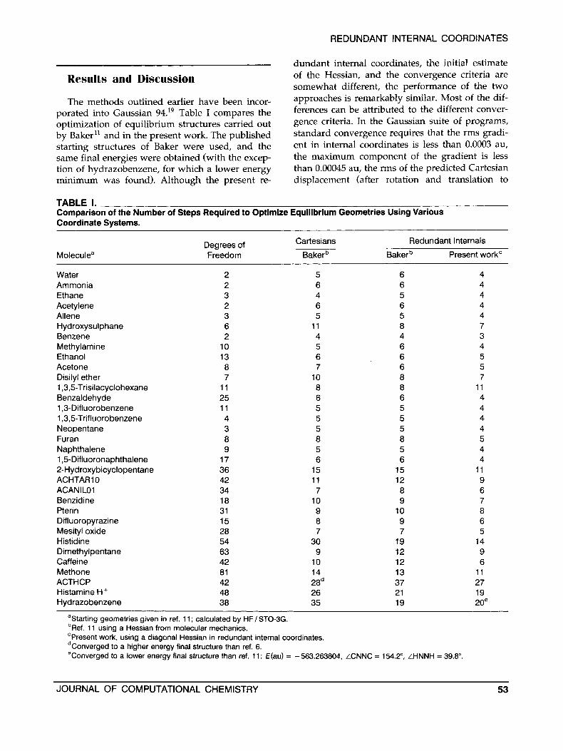
The methods outlined earlier have been incor- porated into Gaussian 94.19 Table I compares the optimization of equilibrium structures carried out by Baker" and in the present work. The published starting structures of Baker were used, and the same final energies were obtained (with the excep- tion of hydrazobenzene, for which a lower energy minimum was found). Although the present re-

of the Hessian, and the convergence criteria are somewhat different, the performance of the two approaches is remarkably similar. Most of the differences can be attributed to the different convergence criteria. In the Gaussian suite of programs, standard convergence requires that the rms gradient in internal coordinates is less than 0.0003 au, the maximum component of the gradient is less than 0.00045 au, the rms of the predicted Cartesian displacement (after rotation and translation to

TABLE I. Comparison of the Number of Steps Required to Optimize Equilibrium Geometries Using Various Coordinate Systems.

Moleculea Degrees of Freedom

Water Ammonia Ethane Acetylene Allene Hydroxysulphane Benzene Methylamine Ethanol Acetone Disilyl ether 1,3,5-Trisilacyclohexane Benzaldehyde 1,3-DifIuorobenzene 1,3,5-TrifIuorobenzene Neopentane Furan Naphthalene 1,5-DifIuoronaphthalene 2-Hydroxybicyclopentane ACHTARlO ACAN ILO1 Benzidine Pterin Difluoropyrazine Mesityl oxide Histidine Dimethylpentane Caffeine Methone ACTHCP Histamine H+ Hydrazobenzene

2 2 3 2 3 6 2

10 13 8 7

11 25 11 4 3 8 9

17 36 42 34 18 31 15 28 54 63 42 81 42 48 38

Cartesians Redundant lnternals

Bakerb Bakerb Present work'

5 6 4 6 6 4 4 5 4 6 6 4 5 5 4

11 8 7 4 4 3 5 6 4 6 6 5 7 6 5

10 8 7 8 8 11 6 6 4 5 5 4 5 5 4 5 5 4 8 8 5 5 5 4 6 6 4

15 15 11 11 12 9 7 8 6

10 9 7 9 10 8 8 9 6 7 7 5

30 19 14 9 12 9

10 12 6 14 13 11 28d 37 27 26 21 19 35 19 2oe

aStarting geometries given in ref. 11 ; calculated by HF/ STO-3G. bRef. 11 using a Hessian from molecular mechanics. 'Present work, using a diagonal Hessian in redundant internal coordinates. dConverged to a higher energy final structure than ref. 6. eConverged to a lower energy final structure than ref. 11: €(ad = -563,263804, LCNNC = 154.2", LHNNH = 39.8".


PENG ET AL.

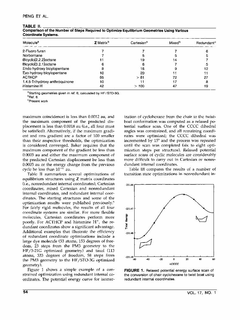
TABLE II. Comparison of the Number of Steps Required to Optimize Equilibrium Geometries Using Various Coordinate Systems.

Moleculea Z Matrix Cartesianb Mixedb Redundant'

2-Fluoro furan Norbornane Bicyclo[2.2.2loctane Bicyclo[3.2.1 ]octane Endo hydroxy bicylopentane Exo hydroxy bicylopentane ACTHCP 1,4,5-Trihydroxy anthroquinone Histamine H+

7 7

11 6 8

10 65 10 42

7 5

19 6

18 20

> 81 11

> 100

7 5

14 7 9

11 72 17 47

6 5 7 5

12 11 27 8

19

aStarting geometries given in ref. 6; calculated by HF / STO-3G. bRef. 6. 'Present work

maximum coincidence) is less than 0.0012 au, and the maximum component of the predicted displacement is less than 0.0018 au (i.e., all four must be satisfied). Alternatively, if the maximum gradient and rms gradient are a factor of 100 smaller than their respective thresholds, the optimization is considered converged. Baker requires that the maximum component of the gradient be less than 0.0003 au and either the maximum component of the predicted Cartesian displacement be less than 0.0003 au or the energy change from the previous cycle be less than au.

Table I1 summarizes several optimizations of equilibrium structures using Z matrix coordinates (i.e., nonredundant internal coordinates), Cartesian coordinates, mixed Cartesian and nonredundant internal coordinates, and redundant internal coordinates. The starting structures and some of the optimization results were published previously.6 For fairly rigid molecules, the results of all four coordinate systems are similar. For more flexible molecules, Cartesian coordinates perform more poorly. For ACTHCP and histamine H+, the redundant coordinates show a significant advantage. Additional examples that illustrate the efficiency of redundant coordinate optimizations include a large dye molecule (53 atoms, 153 degrees of freedom, 23 steps from the PM3 geometry to the HF/3-21G optimized geometry) and taxol (113 atoms, 333 degrees of freedom, 58 steps from the PM3 geometry to the HF/STO-3G optimized geometry).

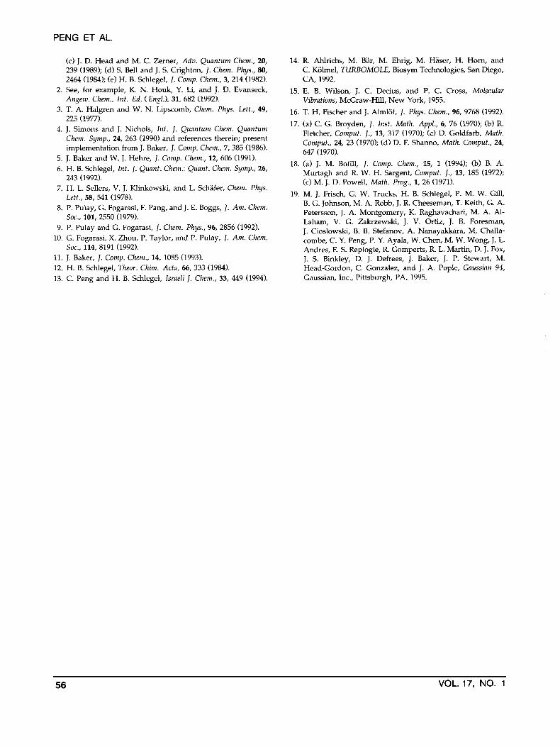
Figure 1 shows a simple example of a constrained optimization using redundant internal coordinates. The potential energy curve for isomer-

ization of cyclohexane from the chair to the twist- boat conformation was computed as a relaxed potential surface scan. One of the CCCC dihedral angles was constrained, and all remaining coordinates were optimized; the CCCC dihedral was incremented by 15" and the process was repeated until the scan was completed (six to eight optimization steps per structure). Relaxed potential surface scans of cyclic molecules are considerably more difficult to carry out in Cartesian or nonredundant internal coordinates.

Table I11 compares the results of a number of transition state optimizations in nonredundant in-

I -231.46

-60 4 -20 0 20 40 60

<cccc

FIGURE 1. Relaxed potential energy surface scan of the conversion of chair cyclohexane to twist boat using redundant internal coordinates.

54 VOL. 17, NO. 1


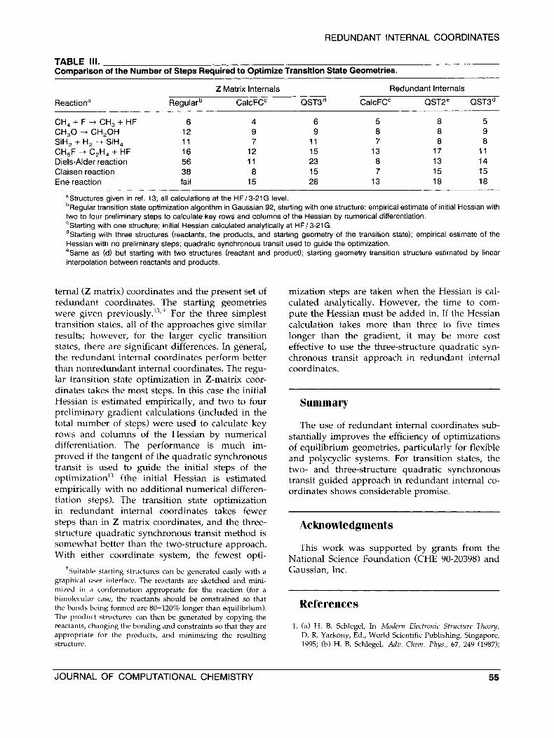
TABLE 111. Comparison of the Number of Steps Required to Optimize Transition State Geometries.

Z Matrix lnternals Redundant lnternals

Reactiona Regularb CalcFC" QST3d CalcFC" QST2e QST3d

CH,+F+ CH,+HF 6 4 6 5 8 5 CH,O + CH,OH 12 9 9 8 8 9

CH,F + C,H, + HF 16 12 15 13 17 11 SiH, + H, --f SiH, 11 7 11 7 8 8

Diels-Alder reaction 56 11 23 8 13 14 Claisen reaction 38 8 15 7 15 15 Ene reaction fail 15 28 13 18 18

aStructures given in ref. 13; all calculations at the HF13-21G level. bRegular transition state optimization algorithm in Gaussian 92, starting with one structure; empirical estimate of initial Hessian with two to four preliminary steps to calculate key rows and columns of the Hessian by numerical differentiation. 'Starting with one structure; initial Hessian calculated analytically at HF/ 3-21 G. Starting with three structures (reactants, the products, and starting geometry of the transition state); empirical estimate of the

Hessian with no preliminary steps; quadratic synchronous transit used to guide the optimization. eSarne as (d) but starting with two structures (reactant and product); starting geometry transition structure estimated by linear interpolation between reactants and products.

ternal (Z matrix) coordinates and the present set of redundant coordinates. The starting geometries were given previo~sly.'~,' For the three simplest transition states, all of the approaches give similar results; however, for the larger cyclic transition states, there are significant differences. In general, the redundant internal coordinates perform better than nonredundant internal coordinates. The regular transition state optimization in Z-matrix coordinates takes the most steps. In this case the initial Hessian is estimated empirically, and two to four preliminary gradient calculations (included in the total number of steps) were used to calculate key rows and columns of the Hessian by numerical differentiation. The performance is much improved if the tangent of the quadratic synchronous transit is used to guide the initial steps of the ~ptimization'~ (the initial Hessian is estimated empirically with no additional numerical differentiation steps). The transition state optimization in redundant internal coordinates takes fewer steps than in Z matrix coordinates, and the three- structure quadratic synchronous transit method is somewhat better than the two-structure approach. With either coordinate system, the fewest opti-

'Suitable starting structures can be generated easily with a graphical user interface. The reactants are sketched and mini- mized in a conformation appropriate for the reaction (for a bimolecular case, the reactants should be constrained so that the bonds being formed are 80-120% longer than equilibrium). The product structures can then be generated by copying the reactants, changing the bonding and constraints so that they are appropriate for the products, and minimizing the resulting structure.

mization steps are taken when the Hessian is calculated analytically. However, the time to com- pute the Hessian must be added in. If the Hessian calculation takes more than three to five times longer than the gradient, it may be more cost effective to use the three-structure quadratic synchronous transit approach in redundant internal coordinates.

Summary

The use of redundant internal coordinates sub- stantially improves the efficiency of optimizations of equilibrium geometries, particularly for flexible and polycyclic systems. For transition states, the two- and three-structure quadratic synchronous transit guided approach in redundant internal coordinates shows considerable promise.

Acknowledgments

This work was supported by grants from the National Science Foundation (CHE 90-20398) and Gaussian, Inc.

References

1. (a) H. B. Schlegel, In Modern Electronic Structure Theory, D. R. Yarkony, Ed., World Scientific Publishing, Singapore, 1995; (b) H. B. Schlegel, Adv. Chem. Phys., 67, 249 (1987);


PENG ET AL.

(c) J. D. Head and M. C. Zemer, A h . Quantum Chem., 20, 239 (1989); (d) S. Bell and J. S. Crighton, 1. Chem. Phys., 80, 2464 (1984); (e) H. B. Schlegel, J . Comp. Chem., 3,214 (1982).

2. See, for example, K. N. Houk, Y. Li, and J. D. Evanseck, Angew. Chem., Int. Ed. (Engl.), 31, 682 (1992).

3. T. A. Halgren and W. N. Lipscomb, Chem. Phys. Lett., 49, 225 (1977).

4. J. Simons and J. Nichols, Int. 1. Quantum Chem. Quantum Chem. Symp., 24, 263 (1990) and references therein; present implementation from J. Baker, J . Comp. Chem., 7,385 (1986).

5. J. Baker and W. J. Hehre, J. Comp. Chem., 12, 606 (1991). 6. H. B. Schlegel, Int. J. Quant. Chem.: Quant. Chem. Symp., 26,

7. H. L. Sellers, V. J. Klinkowski, and L. Schafer, Chem. Phys.

8. P. Pulay, G. Fogarasi, F. Pang, and J. E. Boggs, J . Am. Chem.

9. P. Pulay and G. Fogarasi, J . Chem. Phys., 96, 2856 (1992). 10. G. Fogarasi, X. Zhou, P. Taylor, and P. Pulay, 1. Am. Chem.

11. J. Baker, J. Comp. Chem., 14, 1085 (1993).

243 (1992).

Lett., 58, 541 (1978).

SOC., 101, 2550 (1979).

Soc., 114, 8191 (1992).

14. R. Ahlrichs, M. Bar, M. Ehrig, M. Haser, H. Horn, and C. Kolmel, TURBOMOLE, Biosym Technologies, San Diego, CA, 1992.

15. E. B. Wilson, J. C. Decius, and P. C. Cross, Molecular Vibrations, McGraw-Hill, New York, 1955.

16. T. H. Fischer and J. Almlof, J . Phys. Chem., 96, 9768 (1992). 17. (a) C. G. Broyden, J . Inst. Math. Appl., 6, 76 (1970); (b) R.

Fletcher, Comput. J., 13, 317 (1970); (c) D. Goldfarb, Math. Comput., 24, 23 (1970); (d) D. F. Shanno, Math. Comput., 24, 647 (1970).

18. (a) J. M. Bofill, J. Comp. Chem., 15, 1 (1994); (b) 8. A. Murtagh and R. W. H. Sargent, Comput. J., 13, 185 (1972); (c) M. J. D. Powell, Math. Prog., 1, 26 (1971).

19. M. J. Frisch, G. W. Trucks, H. B. Schlegel, P. M. W. Gill, B. G. Johnson, M. A. Robb, J, R. Cheeseman, T. Keith, G. A. Peterson, J. A. Montgomery, K. Raghavachari, M. A. Al- Laham, V. G. Zakrzewski, J. V. Ortiz, J. 8. Foresman, J. Cioslowski, B. 8. Stefanov, A. Nanayakkara, M. Challa- combe, C. Y. Peng, P. Y. Ayala, W. Chen, M. W. Wong, J. L. Andres, E. S. Replogle, R. Gomperts, R. L. Martin, D. J. Fox, J. S. Binkley, D. J. Defrees, J. Baker, J. P. Stewart, M.

12. H. B. Schlegel, Theor. Chim. Acta, 66, 333 (1984). 13. C. Peng and H. B. Schlegel, Israeli J. Chem., 33, 449 (1994).

Head-Gordon, C. Gonzalez, and J. A. Pople, Gaussian 94, Gaussian, Inc., Pittsburgh, PA, 1995.

56 VOL. 17, NO. 1

Documents

Using redundant internal coordinates to optimize equilibrium geometries and transition states