Using Real Options to Evaluate Producer Investment in New Generation Cooperatives

Thomas L. Sporleder and Michael D. Bailey

Selected Paper American Agricultural Economics Association Annual Meeting

Chicago, IL, August 5 – August 8, 2001

Using Real Options to Evaluate Producer

Investment in New Generation Cooperatives

by

Thomas L. Sporleder and

Michael D. Bailey1

Abstract

New Generation Cooperatives have emerged as a contemporary means for farmers to

invest in further processing activities. This paper considers real options as the basis for evaluating producer investment in a start-up cooperative that involves technological uncertainty. The investment and risk inherent in producer membership in an NGC is analyzed using real options theory logic. Real options theory has recently been extended to technology positioning projects and how the extent of uncertainty influences the value of a technology “option”. Conventional net present value formulas have been shown to be limited when the conditions of the investment require substantial commitment under uncertainty, such as investments in technology.

Implications for producers are drawn from the analysis. Producers always have the alternative of not investing in the initial start-up but waiting and buying in at a later time, perhaps when less uncertainty prevails. Results indicate that producers are better able to evaluate investment in a NGC using real options.

Copyright 2001 by Thomas L. Sporleder and Michael D. Bailey. All rights reserved. Readers may make verbatim copies of this document for non-commercial purposes by any means, provided that this copyright notice appears on all such copies.

Keywords: Real options, New Generation Cooperatives, finance

JEL codes: Q130 and Q140

1 Professor and Farm Income Enhancement Endowed Chair, and Graduate Research Associate, respectively, Department of Agricultural, Environmental, and Development Economics, The Ohio State University.

1

Using Real Options to Evaluate Producer Investment In New Generation Cooperatives

Introduction and Background

For farmers, value added activities usually mean becoming involved in

downstream activities beyond the farm gate, such as further processing. So-called “New

Generation Cooperatives” (NGCs) have emerged as a contemporary means for farmers

invest in further processing activities. NGCs are agricultural marketing cooperatives

engaged in further processing and are designed to serve producers committed to

participating in the cooperative. By design, NGCs have some unique features compared

to traditional agricultural marketing cooperatives. NGCs have closed membership, there

are limits on the amount of commodity that can be accepted from members, and member

investment is tied to patronage rights (rights to deliver commodity to the cooperative).

Unlike a conventional cooperative, patronage rights are transferable at market value when

a producer no longer wishes to be a member of the NGC.

There are important differences in the characteristics of NGC cooperatives and

traditional marketing cooperatives. Up-front investment may be substantial, often as

much as 30 to 50 percent of the cooperative’s total capital needs (Harris et al., 1996).

The initial price of a share in the cooperative is calculated by dividing the total amount of

equity capital necessary by the number of units of commodity the facility will be able to

process. Note that the investment is typically for access to further processing capacity

that also means that the producer is investing in technology embedded within the further

processing facility.

2

The economic problem evaluated by this analysis is the producer investment and risk

associated with an NGC for producers contemplating becoming a member of an NGC.

Fortunately, there is a new means of evaluating this investment and risk that has not been

applied to cooperative membership prior to the current analysis. Real options theory

provides a novel means for understanding producer risk and investment.

The focus of this research is a simulation model that evaluates an Ohio

agricultural producers’ decision to invest in a tortilla chip processing business, which is

formed as a New Generation Cooperative. In order to specifically accomplish this

objective, the task of this research is to simulate the potential producer returns from

membership, calculating both as a traditional net present value and real option value.

Overview of New Generation Cooperatives

In an effort to survive in a highly concentrated and integrated agricultural

environment, there has been an upsurge in cooperative value-added activities throughout

the United States (Torgerson et al., 1998). Two of the most important attributes common

to NGCs are the existence of delivery shares and restricted (closed) membership (Fulton,

2000). Also, the cooperative’s equity shares are transferable between members, and

relatively high levels of cash patronage refunds are issued annually to the producer

(Patrie, 1998).

Membership equity shares, whose sale is used to aid in initially financing the

NGC, obligate not only the member to deliver a commodity to the cooperative, but also

the cooperative to accept the commodity (Harris et al., 1996). In purchasing the

minimum required equity shares, members make a specific capital and commodity

volume commitment to the cooperative (Poray and Ginder, 1999).

3

Overview of Real Option Valuation

The commonly used methodologies that address the critical issues of investment

uncertainty and flexibility are dynamic discounted cash flow analysis, decision analysis,

and option valuation (Teisberg, 1995). This research expressly focuses upon the newest

of the three methodologies, option valuation. Furthermore, this research compares and

contrasts option valuation with static discounted cash flow, or net present value (NPV).

The foundation of real options rests upon mutual characteristics of investment

decisions. Dixit and Pindyck (1994) discuss these aspects, summarizing that the cost of

the investment cannot be completely recovered, the outcomes of the investment are not

known with certainty, and that there is some flexibility surrounding the timing of the

investment.

The main argument of the real option theory is that most investment valuation

techniques do not account for these characteristics. However, by recognizing each of

these attributes of an investment decision, “optimal investment rules can be obtained

from methods that have been developed for pricing options in financial markets (Dixit

and Pindyck, 1994). Ergo, real options theory presumes that financial option valuation

methodology is transferable to and sometimes appropriate for investment valuation.

A clarification of the differences and similarities between real option investment

valuation and conventional decision analysis (NPV) aids in definitional comprehension.

A project’s NPV is the present value of the difference between the project’s value and its

cost. By definition of the NPV rule, managers should accept all projects with a net

present value greater than zero (Brealey et al., 2001).

4

Net present value is commonly used in decision-making. Trigeorgis writes that,

“In the absence of managerial flexibility, net present value (NPV) is the only currently

available valuation measure consistent with a firm’s objective of maximizing its

shareholder’s wealth” (1996, p.25). Furthermore, net present value is generally

considered to be superior to other methods of valuation, such as payback period,

accounting rate of return, and internal rate of return (Trigeorgis,1996).

Conventional capital budgeting only offers decision makers the choice of

investing or not investing (Luehrman, September 1998). A defining distinction between

real options and conventional decision-making is based upon the choices that each

methodology offers. The standard net present value rule does not take into account how

“the ability to delay an irreversible investment expenditure can profoundly affect the

decision to invest” (Dixit and Pindyck, 1994, p.6).

The basic assumptions of real options and net present value, specifically regarding

investment deferral and reversibility, are important for distinction. In their work

Investment Under Uncertainty, Dixit and Pindyck (1994) state that being able to “delay

an irreversible investment…undermines the simple net present value rule, and hence the

theoretical foundation of standard neoclassical investment models.” (p. 6)

Regarding the premise of investment deferral, net present value neither recognizes

nor explicitly accounts for the managerial alternative of waiting, delaying the start of, or

“phasing” the investment of a project. However, real options theory recognizes that a

given investment decision can be deferred (Luehrman, July 1998). Concerning the

assumption of investment reversibility, the NPV rule implicitly assumes that “either the

5

investment is reversible” or “if the investment is irreversible, it is a now or never

proposition” (Dixit and Pindyck, 1994).

The ability to delay or phase an irreversible expenditure involves the issue of

managerial contingency to alter course in the future. This “managerial flexibility” is

important in structuring the project analysis, as such flexibility is often a source of

additional value in the investment decision (Bodie and Merton, 2000, p.450). Therefore,

standard NPV analysis is more than suitable for projects with very little to no uncertainty

(Brennan and Trigeorgis, 2000). Real options theory offers advantages in analyzing

those investment decisions that inherently have significant uncertainty. Flexibility,

within the context of real options applications, is “purchased,…adds value and is very

much sought after”(Glantz, 2000, p.57).

Because of the fundamental differences between conventional decision making

and real options theory, an option approach’s valuation of a sunk cost investment will be

greater than or equal to the value of the NPV approach for the same project. Glantz

(2000) states that net present value essentially disregards any opportunities in investment

analysis to change the “game plan”. Because flexibility is the epitome of real options

theory, NPV consequently underestimates projects that are clearly elastic (Glantz, 2000).

The net result of uncertainty is, by not accounting for “managerial flexibility”, the NPV

of the project will be underestimated relative to the real options approach (Bodie and

Merton 2000, p. 448).

In the absence of uncertainty over time, both the real option value and the net

present value are equal to the present value of the project assets less the expenditure

required to obtain those assets. In options terminology, NPV is equal to the stock price

6

(S) minus the exercise price (E), or NPV = S – E. This similarity aids in clarifying where

option valuation and NPV diverge: the recognition of uncertainty over time with respect

to variability in prices, interest rates, consumer tastes, and technology. Real options

invite managers to account those effects.

Real options are present in numerous investment decisions, and can take many

forms. Trigeorgis (1996) gives many examples, including the staged-investment option,

as well as the option to expand, contract, shutdown, or restart. Also listed is the option to

abandon, as well as the option to switch inputs or outputs.

Real Option Valuation Methodology

In this research, the “real” option refers to the producer’s indirect brick and

mortar investment in the corn tortilla chip processing facilities. Because the

characteristics of a real option are similar to a European call option, investment

techniques from financial markets to value the option are used (Bodie and Merton, 2000).

A sunk investment is analogous to a financial call option: The owner of the option has

the right, but not the obligation, to pay an exercise price for a future investment.

A simplified four-step approach to solving real options applications is proffered

by Amram and Kulatilaka (1999). The broad process includes the initial step of framing

the application, then implementing an option valuation model, reviewing the results, and

redesigning the application as needed.

To quantify the investment payoff to the members of a further processing NGC,

an option valuation model is designed. The approach is based upon the Black-Scholes

option-pricing model (Black and Scholes, May/June 1973). Although other methods of

options value calculation are available, including the Binomial Model, Black-Scholes is

7

the most common method of analytical solutions because of its ease of use (Amram and

Kulatilaka, 1999).

Benninga (2000) points out that, even though the Black-Scholes’ key strength lies

in being numerically tractable, the best that it can give us is a ballpark figure of an

authentic option value. Black-Scholes is limited to providing mere approximations

because of the limitations of its key assumptions, which include continuous trading,

constant interest rate, and no exercise before expiration date (as is the case with

American options) (Benninga, 2000). With such drawbacks being duly noted, the Black-

Scholes formula is still “well suited for simple real options, those with a single source of

uncertainty and a single decision date”(p.36) (Amram and Kulatilaka, 1999).

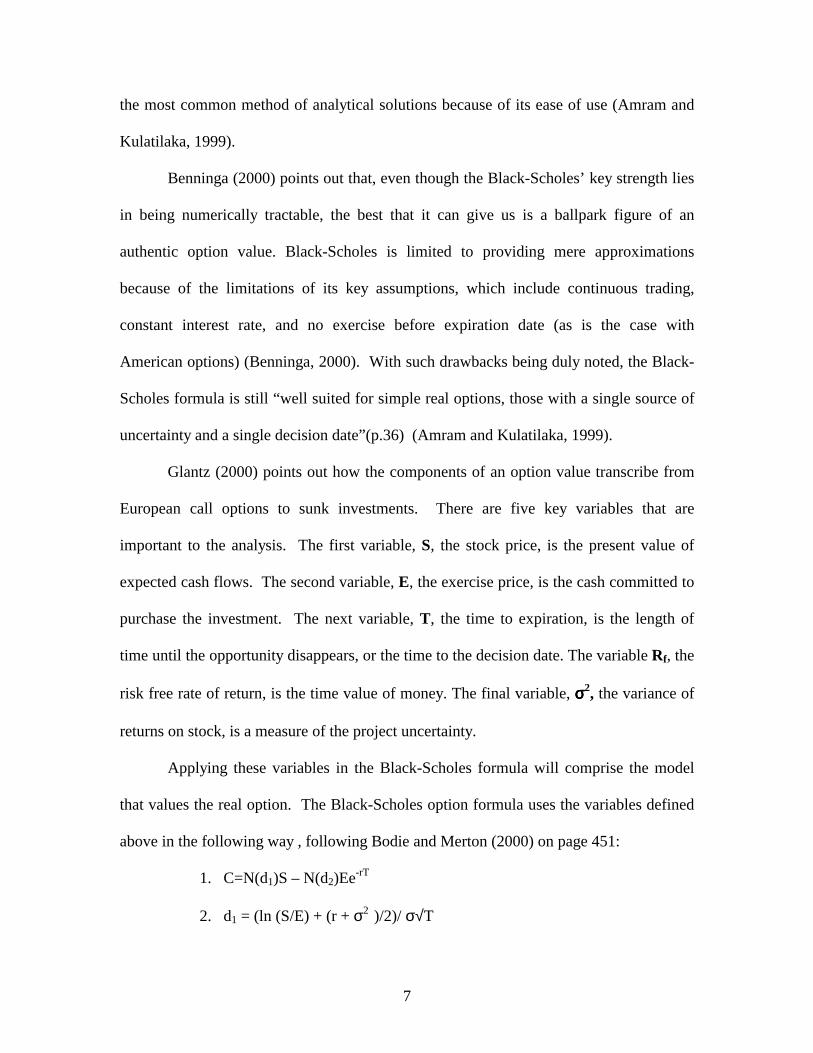
Glantz (2000) points out how the components of an option value transcribe from

European call options to sunk investments. There are five key variables that are

important to the analysis. The first variable, S, the stock price, is the present value of

expected cash flows. The second variable, E, the exercise price, is the cash committed to

purchase the investment. The next variable, T, the time to expiration, is the length of

time until the opportunity disappears, or the time to the decision date. The variable Rf, the

risk free rate of return, is the time value of money. The final variable, σσσσ2, the variance of

returns on stock, is a measure of the project uncertainty.

Applying these variables in the Black-Scholes formula will comprise the model

that values the real option. The Black-Scholes option formula uses the variables defined

above in the following way , following Bodie and Merton (2000) on page 451:

1. C=N(d1)S – N(d2)Ee-rT

2. d1 = (ln (S/E) + (r + σ2 )/2)/ σ√T

8

3. d2 = d1 - σ√T

Amram and Kulatilaka (1999) offer the following interpretation for the groups of

terms in the right-hand side of equation 1: N(d1)S represents the expected value of the

current underlying asset, if the current value is greater than the investment cost at

expiration. N(d2) represents the risk neutral probability that the current value of the

underlying asset will be greater than the cost of investment at expiration. Finally, Ee-rT

represents the present value of the cost of investment. Where E = expenditure required to

acquire the project’s assets and e is the base of the natural logs; r = risk free rate of

return; and T = length of time the decision may be deferred.

As part of the solution methodology, after the application is successfully framed,

and the Black-Scholes model is properly utilized, a subjective credibility check is needed

as well. Such a credibility check is warranted, so as to ascertain whether or not the

computed option values appear to be “realistic” (Amram and Kulatilaka, 1999).

The focus upon option calculation methodology must be kept in relative context.

That is, regardless of the type of option methodology employed, the actual process of

designing and implementing a real options application has as much inherent value in

investment analysis as does the resulting computed option value.

Luehrman (July 1998) stresses this notion, by stating “a naively formulated option

value will augment whatever insight may be drawn from a DCF treatment alone”(p.64).

This augmentation of insight is derived from one key benefit of detailing the option,

which is the identification of risk (Amram and Kulatilaka, 2000). For these reasons, the

use and application of real options should be, in practice, a “complement to existing

capital-budgeting systems, not a substitute for them” (Luehrman, 1998).

9

Investment Deferral and Competitive Preemption

As previously discussed, the real options approach places an economic value on

decision-making flexibility, which is often in the form of an investment option (i.e.

waiting or delaying a decision on investment to some future time period). Because this

research places a great emphasis upon the producers’ option to delay full investment in a

value-added cooperative, it is necessary to address the potential downfalls of waiting to

invest. This discussion focuses on the broader conceptual concerns of real options theory,

especially the theory’s general premise of delaying investment.

Investment deferral, when possible, is not always the correct alternative.

Luehrman points out the possibility that “competitive preemption…would offset some or

all of the sources of value associated with waiting”(July 1998, p.64). The benefits of

waiting must be tempered by the risk of moving too late. In other words, investors

cannot wait indefinitely. Bounds placed on the window of decision-making opportunity

regarding an investment in further processing may involve preemption by other firms, or

other producers purchasing all available stock.

The business literature theory that seems counterintuitive to waiting or delaying

decisions is often called the “first mover” advantage. Nakata and Sivakumar (1997)

suggest that such a first mover advantage can have either preemptive or technological

foundations.

However, there is some disagreement amongst analysts regarding the presence

and effects of first-mover advantage. Lieberman and Montgomery (1988, p.52)

originally indicated that the concept of first-mover advantage may be too general, and its

definition too elusive to be useful. The authors still maintain this notional concern today

10

(Lieberman and Montgomery, 1998). Also, there are opposing viewpoints on whether or

not first mover advantage, if obtained, is sustainable. In a recent study, Makadok (1998)

maintains that first mover and early mover advantages in a market with low barriers to

entry and low barriers to imitation can be sustained. To the contrary, D'aveni (1994)

points out that advantages diminish, because “as competitors copy an advantage, it is no

longer an advantage. It is simply a cost of doing business” (p.233).

Whether or not first-mover advantage is sustainable, the overall concept is vital in

assigning an economic value to investment deferral. With the inclusion of first-mover

advantage, investment timing analysis becomes all the more crucial to project success.

Relevant to the first mover advantage discussion, there are two specific parameters used

in calculating real options value of investments

Competitive Preemption: Black-Scholes’ Variables T and σσσσ

The previously discussed parameters of time (T) and uncertainty (σσσσ) are

implicitly tied to the notion of first mover advantage. Mathematically, a project’s real

option value moves in the same direction as these parameters (Bodie and Merton, 2000).

That is, as uncertainty increases for any given T, as measured by σσσσ, the real option value

increases. Similarly, for any given σσσσ, as T increases, the value of the option increases.

T may be considered as a function of preemption. That is, as managers perceive

the risk of preemption increasing, T decreases, or time to expiration declines for the real

option. By means of assigning a specific value to T in the option calculation process, the

decision-maker is implicitly accounting for competitive pre-emption. As an example, if

the decision maker sets T equal to 3 years, instead of 5, 10, 20, or even 30 years, then she

is recognizing that the decision opportunity has inherent temporal constraints.

11

The variable σσσσ might also be considered as a function of preemption. It is argued

that the value of the variable representing volatility, in some small way, reflects the

relative risks of competitive pre-emption. That is, in less competitive industries wherein

there is less relative risk of pre-emption, the value of σσσσ would most likely be lower.

Conversely, in rapidly evolving and highly competitive environments, the threat of pre-

emption will be reflected in the relatively higher volatility of the underlying asset.

This overall discussion of the timing and uncertainty variables of the Black-

Scholes model, even within these confines of a competitive pre-emption argument, serves

to underscore both the impact and magnitude of responsibly and accurately framing the

entire real options application. The biggest source of error in the real options calculation

process is a poorly designed framework (Amram and Kulatilaka, 1999).

Research Methodology

This research project employs dynamic simulation methodology. Powersim 2.5 is

used to develop a dynamic simulation model. Powersim 2.5 is computer software used to

build a model that represents the elements of a system and how those elements interact

with one another (Swire-Thompson et al., 2000).

Swire-Thompson et al indicate that the development of dynamic economic

simulation software, such as Powersim 2.5, enables managers to experiment with

different investment strategies under a variety of future scenarios (Powersim, 1996).

Powersim 2.5 is used as the model’s foundation because of the software’s ability to

simulate the dynamic complexities of the investment analysis (Powersim, 1996).

In order to meet the objectives of this research, the simulation values of two

model variables are of interest. The first is the auxiliary NPV_INVST, which represents

12

the computed net present value of the investment. The second variable is Invest_as_RO,

which represents the option value of the investment. The resulting values of both

variables are presented in dollars per equity share.

Simulation Model Overview

The simulation model constructed to meet the objectives of this research

ultimately calculates the returns to producers from purchasing equity shares in a New

Generation Cooperative that processes food-grade corn into corn tortilla chips. The

model first estimates the capital requirements for constructing such a plant, and well as

the projected profits from operations. A New Generation Cooperative framework was

constructed around the premise of the corn tortilla chip processing plant.

Once the cooperative framework was constructed and employed, each member’s

investment decision in the cooperative was integrated into the model. The model was

constructed so as to next evaluate the producer investment as a European call option. For

the sake of comparative evaluation, the model was also built so as to simultaneously

calculate the net present value of membership. Lastly, the European call option was

translated into the context of a real option investment valuation. Some of the key

variables of the model are discussed in the following sections.

Real Option Application in Model

The crux of the entire simulation model is the portion dedicated to the investment

valuation. Once the model calculates the co-op’s total capital requirements, the member’s

investment per equity share is computed. The total investment per equity share is based

upon a 50 percent equity capitalization goal, and a minimum requirement of 1000 equity

shares per producer. It is assumed that the total investment required from producers is

13

due from prospective members in two installments. Each value is on a per-equity share,

or per-delivery-bushel basis.

The initial amount (first_installment_per_bu) represents a right to become an

active member in the cooperative, contingent upon the remaining amount being paid

(University of Manitoba, 2001). Upon payment of the second installment

(balance_per_bu), producers are assumed to own full equity shares in the cooperative.

The first installment (first_installment_per_bu) is important for two reasons. On a

tangible level, such an installment can be viewed as “seed money” for the development of

the cooperative (University of Manitoba, 2001). A seed money contribution could be

used for such items as finishing the business plan, writing the prospectus, paying the

overall organizational costs, or finishing the financing work (Patrie, 1998).

On a conceptual level, first_installment_per_bu can be interpreted as an implicit

purchase of a real option. The amount paid now (first_installment_per_bu) purchases a

producer the right to pay the exercise price at a specified date.

In short, this research assumes that the net present value calculation does not allow

for flexibility between installments. Furthermore, the real options framework accounts for

the flexibility to expand (or not) at a later time (Luehrman, July-August, 1998). In this

research, that later time is year t+1.

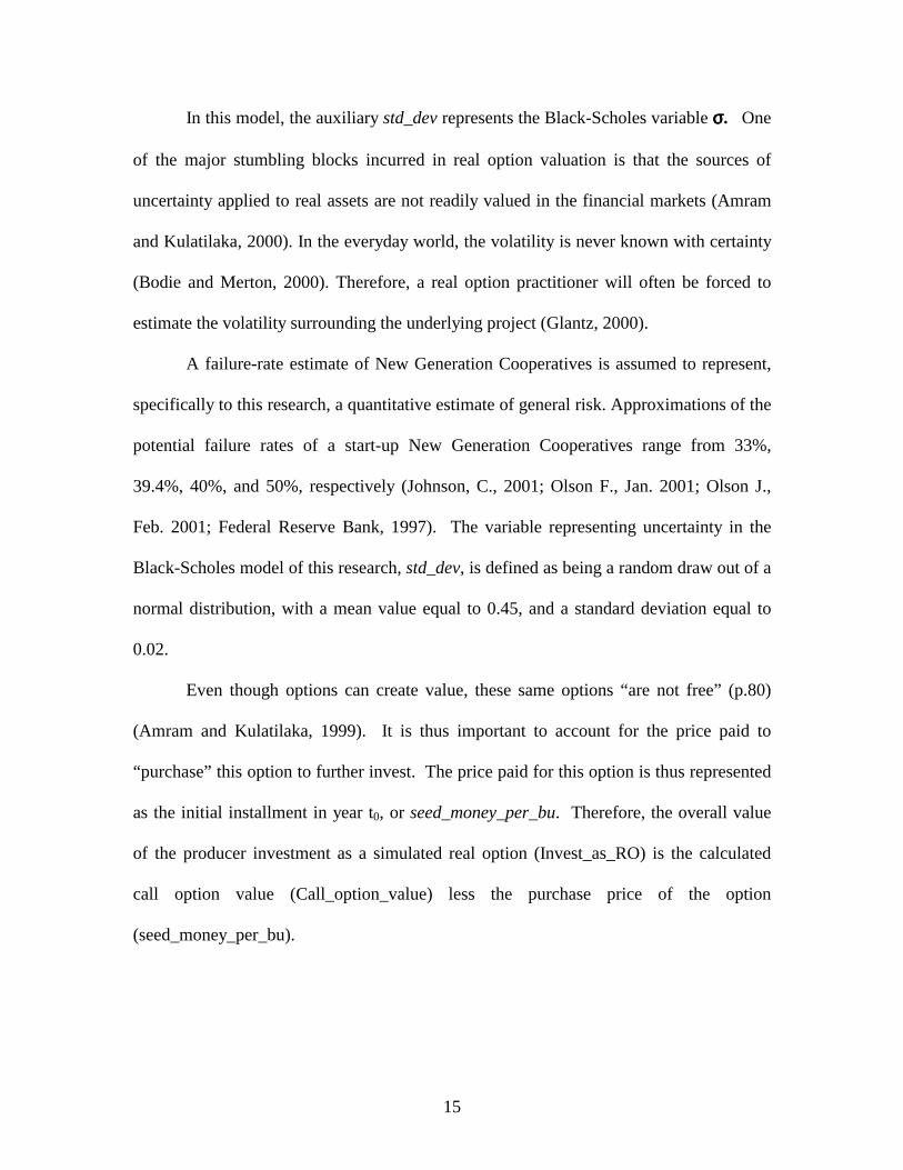
Black-Scholes Variables: E,T,S,Rf, and σσσσ

As is used in the Black-Scholes model, balance_per_bu is considered the exercise

price of the producer investment, or E. The payment of the remaining balance for equity

shares is the exercise price because it represents a specific investment expenditure at a

specified future date t+1. Hence, the value of the option’s expiration, T, is equal to one

14

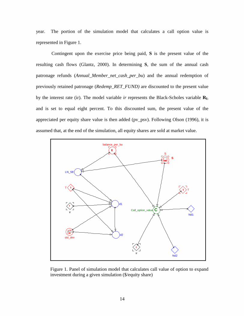
year. The portion of the simulation model that calculates a call option value is

represented in Figure 1.

Contingent upon the exercise price being paid, S is the present value of the

resulting cash flows (Glantz, 2000). In determining S, the sum of the annual cash

patronage refunds (Annual_Member_net_cash_per_bu) and the annual redemption of

previously retained patronage (Redemp_RET_FUND) are discounted to the present value

by the interest rate (ir). The model variable ir represents the Black-Scholes variable Rf,

and is set to equal eight percent. To this discounted sum, the present value of the

appreciated per equity share value is then added (pv_psv). Following Olson (1996), it is

assumed that, at the end of the simulation, all equity shares are sold at market value.

S

t

r

t

r

C

E

ir

ir

T

Nd1

Nd2

d1

d2

LN_SE

balance_per_bu

S

Call_option_value

T

std_dev

Figure 1. Panel of simulation model that calculates call value of option to expand investment during a given simulation ($/equity share)

15

In this model, the auxiliary std_dev represents the Black-Scholes variable σσσσ. One

of the major stumbling blocks incurred in real option valuation is that the sources of

uncertainty applied to real assets are not readily valued in the financial markets (Amram

and Kulatilaka, 2000). In the everyday world, the volatility is never known with certainty

(Bodie and Merton, 2000). Therefore, a real option practitioner will often be forced to

estimate the volatility surrounding the underlying project (Glantz, 2000).

A failure-rate estimate of New Generation Cooperatives is assumed to represent,

specifically to this research, a quantitative estimate of general risk. Approximations of the

potential failure rates of a start-up New Generation Cooperatives range from 33%,

39.4%, 40%, and 50%, respectively (Johnson, C., 2001; Olson F., Jan. 2001; Olson J.,

Feb. 2001; Federal Reserve Bank, 1997). The variable representing uncertainty in the

Black-Scholes model of this research, std_dev, is defined as being a random draw out of a

normal distribution, with a mean value equal to 0.45, and a standard deviation equal to

0.02.

Even though options can create value, these same options “are not free” (p.80)

(Amram and Kulatilaka, 1999). It is thus important to account for the price paid to

“purchase” this option to further invest. The price paid for this option is thus represented

as the initial installment in year t0, or seed_money_per_bu. Therefore, the overall value

of the producer investment as a simulated real option (Invest_as_RO) is the calculated

call option value (Call_option_value) less the purchase price of the option

(seed_money_per_bu).

16

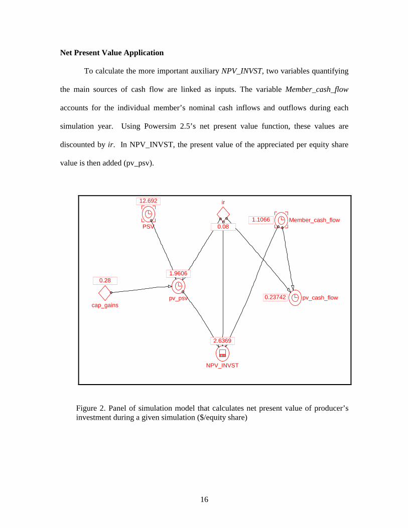
Net Present Value Application

To calculate the more important auxiliary NPV_INVST, two variables quantifying

the main sources of cash flow are linked as inputs. The variable Member_cash_flow

accounts for the individual member’s nominal cash inflows and outflows during each

simulation year. Using Powersim 2.5’s net present value function, these values are

discounted by ir. In NPV_INVST, the present value of the appreciated per equity share

value is then added (pv_psv).

PSV

cap_gains

ir

pv_psv pv_cash_flow

NPV_INVST

Member_cash_flow1.1066

2.6369

0.23742

1.9606

0.08

0.28

12.692

Figure 2. Panel of simulation model that calculates net present value of producer’s investment during a given simulation ($/equity share)

17

Benchmark Simulation Scenario

A most likely simulated scenario is established as a reference scenario. The first

major assumption of the benchmark scenario is that a producer will invest in the New

Generation Cooperative for 20 years (Olson, F., 1996). The NGC is presumed to

construct and operate a four processing line corn tortilla chip processing plant, and meet

50% of its capital needs through member equity. The cooperative will retain 50% of

patronage refunds in the first year, followed by 45 % in the second year, 40% in the third

year, and 35% in the fourth year. Each year thereafter, the cooperative will retain 30% of

retained earnings. It is also assumed that previously retained earnings are returned to the

member on a revolving basis of seven years.

Short Term Investment Horizon Simulation Scenario

The Benchmark simulation scenario assumes that a given producer will invest in

the cooperative for a period of 20 years. A producer must invest in a New Generation

Cooperative for the long-term, as such cooperatives do not presume to swiftly mitigate

the financial strains caused by low commodity prices (Johnson, C., 2001)

Nonetheless, a simulation scenario with an investment horizon of ten years may

yield informative results. The only parameter that distinguishes this scenario from the

benchmark is the length of the investment. One reason cited for the overall lack of

producer equity commitment to the doomed Northern Plains Premium Beef cooperative

was that the value of the investment was not financially lucrative enough to entice the

commitment of older producers who planned to retire within ten years (University of

Manitoba, 2001). Hence, a scenario analysis in this research that evaluates shorter-term

investment horizons is warranted.

18

The length of the investment horizon should not be confused with the option’s

“time until expiration” (T). In this research, the option’s time until expiration does not

change between scenarios. The producer’s opportunity to make the second installment

(balance_per_bu) on equity shares is one year in all cases.

Simulation Results

The computed values of the two auxiliary variables NPV_INVST and

Invest_as_RO are presented and analyzed under each scenario. Under the specified

conditions and assumptions of each scenario, 200 generations of simulations are created

using Powersim 2.5.

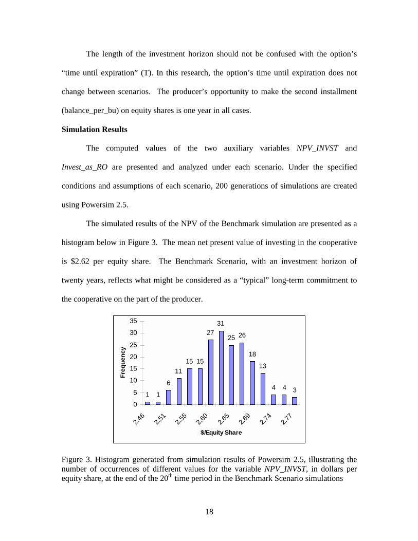
The simulated results of the NPV of the Benchmark simulation are presented as a

histogram below in Figure 3. The mean net present value of investing in the cooperative

is $2.62 per equity share. The Benchmark Scenario, with an investment horizon of

twenty years, reflects what might be considered as a “typical” long-term commitment to

the cooperative on the part of the producer.

1 1

6

1115 15

2731

25 26

18

13

4 4 3

0

5

10

15

20

25

30

35

2.46

2.51

2.55

2.60

2.65

2.69

2.74

2.77

$/Equity Share

Freq

uenc

y

Figure 3. Histogram generated from simulation results of Powersim 2.5, illustrating the number of occurrences of different values for the variable NPV_INVST, in dollars per equity share, at the end of the 20th time period in the Benchmark Scenario simulations

19

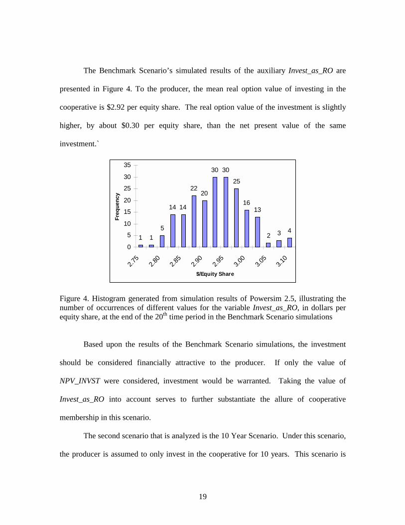
The Benchmark Scenario’s simulated results of the auxiliary Invest_as_RO are

presented in Figure 4. To the producer, the mean real option value of investing in the

cooperative is $2.92 per equity share. The real option value of the investment is slightly

higher, by about $0.30 per equity share, than the net present value of the same

investment.`

1 15

14 14

2220

30 30

25

1613

2 3 4

0

5

10

15

20

25

30

35

2.75

2.80

2.85

2.90

2.95

3.00

3.05

3.10

$/Equity Share

Freq

uenc

y

Figure 4. Histogram generated from simulation results of Powersim 2.5, illustrating the number of occurrences of different values for the variable Invest_as_RO, in dollars per equity share, at the end of the 20th time period in the Benchmark Scenario simulations

Based upon the results of the Benchmark Scenario simulations, the investment

should be considered financially attractive to the producer. If only the value of

NPV_INVST were considered, investment would be warranted. Taking the value of

Invest_as_RO into account serves to further substantiate the allure of cooperative

membership in this scenario.

The second scenario that is analyzed is the 10 Year Scenario. Under this scenario,

the producer is assumed to only invest in the cooperative for 10 years. This scenario is

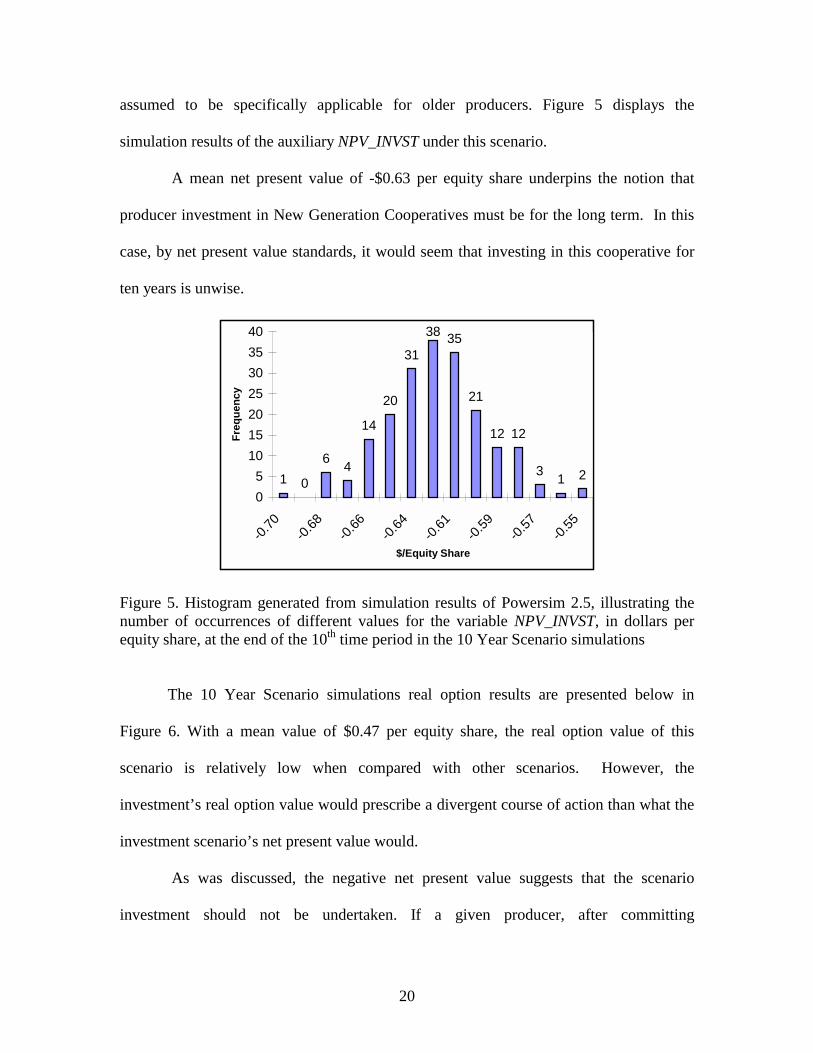
20

assumed to be specifically applicable for older producers. Figure 5 displays the

simulation results of the auxiliary NPV_INVST under this scenario.

A mean net present value of -$0.63 per equity share underpins the notion that

producer investment in New Generation Cooperatives must be for the long term. In this

case, by net present value standards, it would seem that investing in this cooperative for

ten years is unwise.

1 0

6 4

14

20

31

38 35

21

12 12

3 1 205

10152025303540

-0.70

-0.68

-0.66

-0.64

-0.61

-0.59

-0.57

-0.55

$/Equity Share

Freq

uenc

y

Figure 5. Histogram generated from simulation results of Powersim 2.5, illustrating the number of occurrences of different values for the variable NPV_INVST, in dollars per equity share, at the end of the 10th time period in the 10 Year Scenario simulations

The 10 Year Scenario simulations real option results are presented below in

Figure 6. With a mean value of $0.47 per equity share, the real option value of this

scenario is relatively low when compared with other scenarios. However, the

investment’s real option value would prescribe a divergent course of action than what the

investment scenario’s net present value would.

As was discussed, the negative net present value suggests that the scenario

investment should not be undertaken. If a given producer, after committing

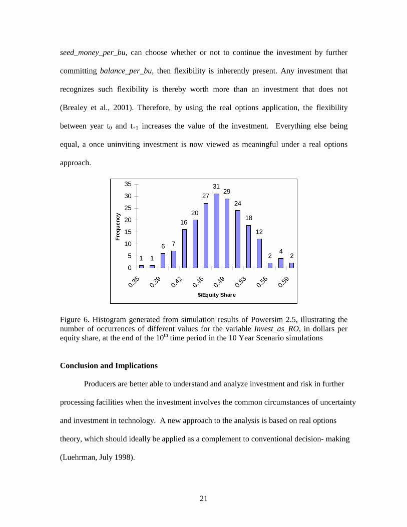
21

seed_money_per_bu, can choose whether or not to continue the investment by further

committing balance_per_bu, then flexibility is inherently present. Any investment that

recognizes such flexibility is thereby worth more than an investment that does not

(Brealey et al., 2001). Therefore, by using the real options application, the flexibility

between year t0 and t+1 increases the value of the investment. Everything else being

equal, a once uninviting investment is now viewed as meaningful under a real options

approach.

1 1

6 7

1620

2731

29

24

18

12

24

2

0

5

10

15

20

25

30

35

0.35

0.39

0.42

0.46

0.49

0.53

0.56

0.59

$/Equity Share

Freq

uenc

y

Figure 6. Histogram generated from simulation results of Powersim 2.5, illustrating the number of occurrences of different values for the variable Invest_as_RO, in dollars per equity share, at the end of the 10th time period in the 10 Year Scenario simulations

Conclusion and Implications

Producers are better able to understand and analyze investment and risk in further

processing facilities when the investment involves the common circumstances of uncertainty

and investment in technology. A new approach to the analysis is based on real options

theory, which should ideally be applied as a complement to conventional decision- making

(Luehrman, July 1998).

22

The generalized framework is illustrated with several numeric examples. Implications are

drawn from the real options model and for conventional mean-variance and net present value

formula evaluations of investment.

Based upon the simulation results, a new generation tortilla chip-processing

cooperative appears to be a feasible alternative for Ohio producers. Both the real option

and net present value of the Benchmark Scenario project a value of at least $2.62 per

equity share

Because the investment decision is set up in two phases, the producer has the

flexibility to discontinue the entire investment at the beginning of the second phase (year

t+1). If a real options analysis were not applied, the investor would forgo the opportunity

to evaluate newer information that might alter the investment strategy (Glantz, 2000).

Because a real options analysis is used, outlay flexibility adds value to the

investment. Therefore, the mean simulated real option value of the 10 Year Scenario is

almost $500 for a minimal investment of 1,000 shares.

This research applied a financial evaluation of producer investment in a New

Generation Cooperative. There is a multitude of other factors that a prospective member

must evaluate. These include the impact that membership in the cooperative may have

on the daily operation of the producer’s farm business, as well as the producer’s personal

goals (Olson, F. March, 1998). Because these considerations are not accounted for in this

research, the economic value of the investment must be tempered with a broader, and

more subjective, analysis. The results of a thorough financial assessment of membership

might recommend action that is in direct contradiction to what is in the best interest of the

producer’s farm operation.

23

Nonetheless, several implications can be derived from the results of this scenario.

First of all, the knowledge of the entire investment has been amplified by the real options

application (Luehrman, July 1998). Also of importance, areas of risk in the investment

have been identified (Amram and Kulatilaka, 2000). By using the real options

application, a once uninviting investment may now be seen as valuable.

REFERENCES Amram, Martha, and Nalin Kulatilaka. 1999. Real Options: Managing Strategic

Investment in an Uncertain World. Harvard Business School Press. Boston, Massachusetts.

Amram, Martha, and Nalin Kulatilaka. 2000. “Strategy and Shareholder Value Creation:

The Real Options Frontier.” Journal of Applied Corporate Finance. Volume 13 (Summer 2000): 89-99.

Benninga, Simon. 2000. Financial Modeling. 2nd Ed. Massachusetts Institute of

Technology. Cambridge, Massachusetts. Black, F., and Myron Scholes. 1973. “The Pricing of Options and Other Corporate

Liabilities.” Journal of Political Economy, 81 (May/June 1973) Bodie, Z. and R.C. Merton. 2000. Finance. Prentice Hall. Upper Saddle River, New

Jersey. Brealey, R., S. Myers, and A. Marcus. 2001. Fundamentals of Corporate Finance.

McGraw-Hill Irwin. Boston, MA. Brennan, Michael J., and Lenos Trigeorgis. 2000. Project Flexibility, Agency, and

Competition. Oxford University Press. New York, New York. D’Aveni, R. A. 1994. Hypercompetition: Managing the Dynamics of Strategic

Maneuvering. Free Press, New York. Dixit, A. and R.S. Pindyck. 1994. Investment under Uncertainty. Princeton University

Press. Princeton, New Jersey. Fulton, Murray. Dec. 2, 2000. “New Generation Cooperatives.” Paper Prepared for

Presentation to seminar entitled Legal Awareness for Specialty Ag Products. Alberta Agriculture, Food, and Rural Development. Edmonton, Alberta

24

Glantz, Morton. 2000. Scientific Financial Management. American Management

Association. New York. Harris, Andrea, Stefanson, Brenda, and Murray Fulton. 1996. “New Generation

Cooperatives and Cooperative Theory.” Journal of Cooperatives. 11 (1996):15-27.

Johnson, Charles. "Added Value, Added Risk.” CPM/Crop Production Magazine.

January, 2001. Volume 14(1):10-11 Lieberman, M.B. and D.B. Montgomery. 1988. “First-mover a1dvantages.” Strategic

Management Journal. Summer Special Issue, 9:41-58. Lieberman, M.B. and D.B. Montgomery. 1998. “First-mover (dis)advantages:

Retrospective and Link with the Resource-based view.” Strategic Management Journal. Volume 19:1111-1125.

Luehrman, Timothy A. 1998. “Investment Opportunities as Real Options: Getting

Started On the Numbers.” Harvard Business Review. July-August 1998:51-67. Luehrman, Timothy A. 1998.“Strategy as a Portfolio of Real Options.” Harvard

Business Review. September-October 1998:89-99. Makadok, Richard. 1998. “Can First-Mover and Early-Mover Advantages Be Sustained

In an Industry with Low Barriers to Entry/Imitation?” Strategic Management Journal. Volume 19:683-696.

Nakata, Cheryl and K. Sivakumar. 1997. “Emerging Market Conditions and Their

Impact on First Mover Advantages: An Integrative Review.” International Marketing Review. Volume 14:461-485.

Olson, Frayne. July, 1996. “Should I Join a New Processing Cooperative?” Extension

Bulletin No 67. North Dakota State University Extension Service. Fargo, ND. Olson, Frayne. January 5, 2001. Personal Correspondence. Olson, Joan. “High Hopes, High Risk.” Farm Industry News. Februrary, 2001:54-68. Patrie, William. 1998. “Creating ‘Co-op Fever’: A Rural Developer’s Guide to Forming

Cooperatives.” Rural Business Cooperative Service. Poray, Michael, and Roger C. Ginder. 1999. “Comparing Alternative Closed Swine

Cooperatives: Adding Value to Corn Under Uncertainty.” Journal of Cooperatives. Volume 14:1-20

25

Powersim Corporation. 1996. “Powersim 2.5 User’s Guide.” PowerSim Press. Herndon, Virginia.

Swire-Thompson, A.P. 2000. Master’s Thesis. The Ohio State University Teisberg, Elizabeth Olmsted. 1995. In Lenos Trigeorgis (ed). “Methods for Evaluating

Capital Investment Decisions under Uncertainty.” Real Options in Capital Investment: Models, Strategies, and Applications. Praeger.

The Federal Reserve Bank. FRB Cleveland. December 1997. Torgerson, Randall, Reynolds, Bruce, and Thomas W. Gray.1998. “Evolution of

Cooperative Thought, Theory, and Purpose.” Journal of Cooperatives. Volume 13:1-17

Trigeorgis, Lenos. 1996. “Real Options”. The MIT Press. Cambridge, Massachusetts University of Manitoba. 2001. “New Generation Cooperatives on the Northern Plains: A

New Generation of Cooperatives.” http://www.umanitoba.ca/afs/agric_economics/ardi.