Using Probabilistic Models for Data Management inAcquisitional Environments

Amol Deshpande∗ Carlos Guestrin∗ Samuel R. MaddenUniversity of Maryland CMU MIT

amol@cs.umd.edu guestrin@cs.cmu.edu madden@csail.mit.edu

There exists a black kingdom which the eyes of man avoidbecause its landscape fails signally to flatter them. This dark-ness, which he imagines he can dispense with in describing thelight, is error with its unknown characteristics... Error is cer-tainty’s constant companion. Error is the corollary of evidence.And anything said about truth may equally well be said abouterror: the delusion will be no greater.

(Prefaceto a Modern Mythology, Louis Aragon, French Poet, 1926.)

Abstract

Traditional database systems, particularly those fo-cused on capturing and managing data from the realworld, are poorly equipped to deal with the noise,loss, and uncertainty in data. We discuss a suiteof techniques based on probabilistic models thatare designed to allow database to tolerate noise andloss. These techniques are based on exploiting cor-relations to predict missing values and identify out-liers. Interestingly, correlations also provide a wayto give approximate answers to users at a signifi-cantly lower cost and enable a range of new typesof queries over the correlation structure itself. Weillustrate a host of applications for our new tech-niques and queries, ranging from sensor networksto network monitoring to data stream management.We also present a unified architecture for integrat-ing such models into database systems, focusing inparticular onacquisitional systemswhere the costof capturing data (e.g., from sensors) is itself a sig-nificant part of the query processing cost.

1 IntroductionThe vision of ubiquitous computing promises to spread in-formation technology throughout our lives. Though this vi-sion can be compelling, it also threatens to overwhelm uswith a flood of information, much of which is spurious,irrelevant, or misleading. Thus, the challenge of realiz-ing this vision is separating the relevant, timely, and use-

∗Work done while the authors were visiting Intel Research Berkeley.

Permission to copy without fee all or part of this material is granted pro-vided that the copies are not made or distributed for direct commercialadvantage, the VLDB copyright notice and the title of the publication andits date appear, and notice is given that copying is by permission of the VeryLarge Data Base Endowment. To copy otherwise, or to republish, requiresa fee and/or special permission from the Endowment.

Proceedings of the 2005 CIDR Conference

ful information out of this flood of data. The data man-agement community has made significant progress towardsachieving this goal – by providing tools that load and cleanthe data, languages and systems that can query the data(e.g.,[52, 36, 10, 38]), and algorithms that mine the data forpatterns and relationships that are of interest [33].

These efforts have largely been focused on mitigatingdata complexity once it has been captured and stored insideof a traditional computing infrastructure. In contrast, we arefocusing on techniques designed to take an active role inmanaging this wealth of data by managing when, where, andwith what frequency data is acquired from distributed infor-mation systems. There are many modern systems where thecapability of local nodes to generate data far outstrips theresources available to transmit or store that data. Nodes in asensor network, for example, typically have processors thatrun at several megahertz, with data collection hardware ca-pable of collecting many kilosamples per second, but radiosthat only transmit kilobytes per second aggregate across allof the nodes in the network. Worse yet, these nodes are bat-tery powered, and, when sampling at maximum rates, onlyhave sufficient energy to last for a few days [46]. Similarly,routers on the Internet can produce huge amounts of net-work monitoring traffic, so much so that the links which thattraffic is transmitted across can be easily saturated. Admin-istrators of large networks typically apply simple techniques(like random sampling) to choose which statistics to col-lect [40]. Streaming database systems have much the sameproblem, where the need to shed load [10] and drop or ag-gregate historical data [52] has been noted.

In addition to the challenges presented by limited re-sources, data from real world environments is often noisy,lossy, and hard to interpret. This noise and uncertaintycan be misleading, particularly when the user is summariz-ing and aggregating data using a high-level language likeSQL. For example, the California Department of Transporta-tion maintains a database of current road speeds from about10,000 traffic sensors on California highways [9]. On a re-cent visit to their website, 60% of sensors were missing data.Such loss could cause users’ queries to pick congested routesif sensors on those routes happen to be offline. If the querysystem could insteadinfer that missing speeds along cer-tain routes are likely to be slow based on past behavior orspeeds from online sensors, query results would be muchmore likely to reflect reality.

Besides failures, real-world networks often produce data

that is simply wrong. For example, in a sensor net-work deployment on Great Duck Island (off the coast ofMaine) [63, 48], researchers noted that about 40% of thesensors produced erratic temperature and humidity readingsat some point; though such readings sometimes precipitatednode failure, in other cases nodes otherwise continued tofunction normally. If the data acquisition system could de-tect and filter such outliers, it could inform a user of thefailure and conserve bandwidth being used to transmit badreadings.

We address all of these problems by building amodelofthe world as data is collected from it. This model allowsus to capture the correlations and statistical relationships be-tween attributes collected by devices. We focus onproba-bilistic models, where the value of each attribute (e.g., tem-perature, light) is a probability distribution that reflects themost likely value of that attribute, possibly depending on thevalues of other attributes (theirdependents), such as the timeof day or behavior of another node in the network. Such de-pendencies, orcorrelations, can be exploited to efficientlyanswer queries and enable new query types that explore therelationships between attributes. Models are built by peri-odically observingvalues of one or more attributes (e.g., byacquiring a reading from a sensor) and using those observa-tions to adjust the probability distributions of the observedattributes and their dependees. Models offer three distinctbenefits:

1. They make queryingmore efficient. By exploiting cor-relations between attributes, it is often possible to useobservations of a small number of attributes to provideapproximations of the values of a large number of at-tributes. For example, if several temperature sensorsin a building read approximately the same temperatureday after day, a good (though perhaps not 100% accu-rate) guess after observing one sensor would be that allof the other sensors have about the same value.

2. They allow the database system to provideprobabilis-tic guarantees on the correctness of answers.Unlikeexisting database systems, which provide the illusion ofprecise answers, even when data is missing or nodes arefaulty, probabilistic models provide probabilistic guar-antees on answers, telling the user the probability thata particular attribute value differs by more than someεfrom the reported value based on past observations orknown values of other, correlated attributes.

3. They allow the database system to answernew types ofqueries. For example, a model can detect certain veryunlikely values (again, by observing past correlationswith other sensors) and flag them as potentialoutliers.Similarly, a model can reveal relationships between de-vices that indicate, for example, that a particular sensoris redundant or that a pair of network links are in noway independent of each other. Finally, a model canoftenpredict the value of a particular attribute as somepoint of time in the past or future.

In this paper, we briefly summarize one model, calledBBQ [22] which we have studied in detail to provide effi-

cient query answers in sensor networks. We then show howour ideas can be generalized to provide the other advantagesdescribed above (e.g., various kinds of probabilistic guaran-tees and support for new types of queries) in a variety ofdomains and applications beyond sensor networks. We ar-gue that any resource limited environment can benefit fromour techniques.

We also show how to adapt a range of techniques, basedon ideas from the machine learning and data mining com-munities, that allow us to improve the predictive power ofmodels, represent correlations more compactly, and selectand train models that are most appropriate for the data beingmodeled. Though such techniques sometimes are directlytransferable from these other domains, they often requiresignificant re-tooling to deal with limited resources, data ac-quisition issues, and to enable integration into a SQL-baseddatabase system.

2 BackgroundIn this section, we summarize the basics of probabilisticmodels and show how they can be used to answer queries.We also summarize our previous work on the BBQ system,which is an example of a probabilistic model tuned to effi-ciently collect data from a sensor network.

2.1 Probabilistic models

We denote a model as aprobability density function(pdf),p(X1, X2, . . . , Xn), assigning a probability for each possi-ble assignment to the attributesX1, . . . , Xn, where eachXi

is an attribute at a particular sensor (e.g., temperature on sen-sor number 5, bandwidth on link A-B). This model can alsoincorporatehidden variables(i.e., variables that are not di-rectly observable) that indicate, for example, whether a sen-sor is giving faulty values or a node is subject to a denial ofservice attack. Such models can be learned from historicaldata using standard algorithms (e.g., [50]).

Answering queries probabilistically based on a pdf isconceptually straightforward. Suppose, for example, thata query asks for an approximation to the value of a set ofattributes to within±ε of the true value of each attribute,with confidence (i.e., probability of being correct) at least1−δ. Using standard probability theory, we can use this pdfto compute the expected value,µi, of each attribute in thequery. These will be our reported values. We can then usethe pdf again to compute the probability thatXi is within εfrom the mean,P (Xi ∈ [µi−ε, µi +ε]). If all of these prob-abilities meet or exceed user specified confidence threshold,then the requested readings can be directly reported as themeansµi. If the model’s confidence is too low, then we re-quire additional readings before answering the query.

Choosing which readings to observe at this point is anoptimization problem: the goal is to pick the best set of at-tributes to observe, minimizing the cost of observation re-quired to bring the model’s confidence up to the user speci-fied threshold for all of the query predicates.

We can use the same technique to compute the expectedsum or average of several attributes (e.g., temperature onk different sensors) by exploiting linearity of expectation,

which saysE(A1 + . . . + Ak) = E(A1) + . . . + E(Ak)and using the standard expression for the variance(σ) of asum to compute ourε, δ bound,i.e., σ(A1 + . . . + Ak) =∑k

i=1 σ(Ai) +∑k

i=1

∑kj=1 cov(Ai, Aj). We can also com-

pute a confidence that a particular boolean predicate (e.g.,temp> 25) is true by integrating over area of the pdf repre-senting the region where the predicate is satisfied.

2.2 Example: Gaussians

In this section, we describe the time-varying multivariateGaussians as a type of model. This is the basic model usedin BBQ [21], and we summarize it here to provide a con-crete example of one kind of model. A multivariate Gaus-sian (hereafter, just Gaussian) is the natural extension ofthe familiar unidimensional normal probability density func-tion (pdf), known as the “bell curve”. Just as with its 1-dimensional counterpart, a Gaussian pdf overd attributes,X1, . . . , Xd can be expressed as a function of two parame-ters: a length-d vector of means,µ, and ad × d matrix ofcovariances,Σ. Figure 1(A) shows a three-dimensional ren-dering of a Gaussian over two attributes,X1 andX2; the zaxis represents thejoint densitythatX2 = x andX1 = y.Figure 1(B) shows a contour plot representation of the sameGaussian, where each circle represents a probability densitycontour (corresponding to the height of the plot in (A)).

Intuitively, µ is the point at the center of this probabilitydistribution, andΣ represents the spread of the distribution.The ith element along the diagonal ofΣ is simply the vari-ance ofXi. Each off-diagonal elementΣ[i, j], i 6= j rep-resents the covariance between attributesXi andXj . Co-variance is a measure of correlation between a pair of at-tributes. A high absolute covariance means that the attributesare strongly correlated: knowledge of one closely constrainsthe value of the other. The Gaussians shown in Figure 1(A)and (B) have a high covariance betweenX1 andX2. Noticethat the contours are elliptical such that knowledge of onevariable constrains the value of the other to a narrow proba-bility band.

We can use historical data to construct the initial rep-resentation of this pdfp. This historical data is typi-cally collected as a part of a short observation phase usingdata extraction tools (in the case of our sensornet deploy-ments, we have typically used a simple selection query inTinyDB [47]). Once our initialp is constructed, we cananswer queries using the model, updating it as new ob-servations are obtained from the sensor network, and astime passes. We explain the details of how updates aredone in Section 2.2.2, but illustrate it graphically with our2-dimensional Gaussian in Figures 1(B) - 1(D). Supposethat we have an initial Gaussian shown in Figure 1(B) andwe choose to observe the variableX1; given the result-ing single value ofX1 = x, the points along the line{(x,X2) | ∀X2 ∈ [−∞,∞]} conveniently form an (unnor-malized) one-dimensional Gaussian. After re-normalizingthese points (to make the area under the curve equal 1.0), wecan derive a new pdf representingp(X2 | X1 = x), whichis shown in 1(C). Note that the mean ofX2 given the valueof X1 is not the same as the prior mean ofX2 in 1(B). Then,

5 10 15 20 25 30 35 40

5

10

15

20

25

30

35

40

X2

X 1

Gaussian PDF over X1,X2 where Σ(X1,X2) is Highly Positive

µ=20,20

5 10 15 20 25 30 35 40

5

10

15

20

25

30

35

40Gaussian PDF over X1, X2 after Some Time

X2

X 1

µ=25,25

5 10 15 20 25 30 350

0.02

0.04

0.06

0.08

0.1

0.12

0.14PDF over X2 After Conditioning on X1

Prob

abilit

y(X 2 =

x)

X2

µ=19

010

2030

40

010

2030

400

0.020.040.060.08

0.10.120.14

X1

2D Gaussian PDF With High Covariance (!)

X2

0.02

0.04

0.06

0.08

0.1

0.12

(C)

(A)

(B)

(D)

Figure 1: Example of Gaussians: (a) 3D plot of a 2D Gaussianwith high covariance; (b) the same Gaussian viewed as a contourplot; (c) the resulting Gaussian overX2 after a particular value ofX1 has been observed; finally, (d) shows how, as uncertainty aboutX1 increases from the time we last observed it, we again have a 2DGaussian with a lower variance and shifted mean.

after some time has passed, our belief aboutX1’s value willbe “spread out”, and we will again have a Gaussian over twoattributes, although the mean and variance may have shiftedfrom their initial values, as in Figure 1(D).

Of course, this is but one example of many different typesof models that could be used. Our basic approach can begeneralized to various different models that may be moresuitable in different environments and for different classesof queries. We will revisit this issue in Section 5. In thenext two sections we look briefly at some of the technicaldetails involved in creating and maintaining the Gaussianmodel used in BBQ.

2.2.1 Learning the model

Typically, probabilistic models are learned from some set oftraining data. In BBQ, this training data consisted of read-ings from all of the monitored attributes over some period oftime. For example, with a Gaussian model, initial means andcovariances can be computed from training data using stan-dard statistical algorithms. Thus, for the specific model usedin BBQ, we need to capture training data for some periodof time before we can begin predicting values or exploit-ing correlations to avoid unneeded acquisitions. We are ex-ploring techniques for interleaving model construction andquery processing when possible, as described in Section 6below.

2.2.2 Updating the model

Thus far, the model we have described representsspatialcorrelation in a network deployment. However, many real-world systems include attributes that evolve over time. Forexample, in a sensor network deployment in our lab, wenoted that the temperatures have both temporal and spa-tial correlations [19]. Thus, the temperature values ob-served earlier in time should help us estimate the temper-

ature later in time. Adynamic probabilistic modelcan rep-resent such temporal correlations by describing the evolu-tion of this system over time, telling us how to computep(Xt+1

1 , . . . , Xt+1n | o1...t) from p(Xt

1, . . . , Xtn | o1...t),

whereo1...t is the set of observations made over the networkup to timet.

One common dynamic model is aMarkovian model,where given the value ofall attributes at timet, the valueof the attributes at timet + 1 are independent of those forany time earlier thant. This assumption leads to a sim-ple model for a dynamic system where the dynamics aresummarized by a conditional density called thetransitionmodel, p(Xt+1

1 , . . . , Xt+1n | Xt

1, . . . , Xtn). Using a transi-

tion model, we can computep(Xt+11 , . . . , Xt+1

n | o1...t) us-ing the standard probabilistic technique ofmarginalizationby integrating the transition model over the attribute valuesat timet.

This approach assumes the transition model is the samefor all timest. Often, this is not the case – for example, inan outdoor environment, in the mornings temperatures tendto increase, while at night they tend to decrease. This sug-gests that the transition model should be different at differ-ent times of the day. One way to address this problem is bylearning a different transition modelpi(Xt+1 | Xt) for eachhour i of the day. At a particular timet, we simply use thetransition modelmod(t, 24). This idea can, of course, begeneralized to other cyclic variations.

Once we have obtainedp(Xt+11 , . . . , Xt+1

n | o1...t),the prior pdf for timet + 1, we can again incorporatethe measurementsot+1 made at timet + 1 obtainingp(Xt+1

1 , . . . , Xt+1n | o1...t+1), the posterior distribution at

time t + 1 given all measurements made up to timet + 1.This process is then repeated for timet + 2, and so on. Thepdf for the initial timet = 0, p(X0

1 , . . . , X0n), is initialized

with the prior distribution for attributesX1, . . . , Xn.

2.3 Architecture

Given this basic structure for models, we show how they fitinto a probabilistic query answering architecture. Parts ofthis architecture were laid out in our work on BBQ [22],though we have extended the architecture here to supportseveral new kinds of queries as described in Section 4 be-low. One of our specific goals is for our architecture to bemodel-agnostic,i.e., as long as a new model conforms to abasic interface, it requires no changes to the query proces-sor and can reuse the code that interfaces with and acquiresparticular tuples.

Figure 2 illustrates our basic architecture through an ex-ample of a probabilistic model running over a sensor net-work. For other environments that involve data acquisition(as we note in Section 3 below), this basic architecture ap-plies unchanged, with the main difference being the dataacquisition mechanism. In non-acquisitional environments,models can still play an important role, as we note in Section3.

Users submit queries to the database as in a traditionaldatabase, though we allow some unusual types of queries(see Section 4). One such class of queries is standard SQL

Probabilistic Model and Planner

Observation Plan

Probabilistic Queries Query Results

Query Processor

"SELECT nodeId, temp ± .1°C, conf(.95) WHERE nodeID in {1..8}"

"1, 22.3 97% 2, 25.6 99% 3, 24.4 95% 4, 22.1 100% ..."

"{[voltage,1], [voltage,2], [temp,4]}"

Data"1, voltage = 2.73 2, voltage = 2.65 4, temp = 22.1"

1

2

3

4

5 6

7

8

Sensor Network

202224262830

1 2 3 4

Sensor ID

Cel

sius

User

Predicate Checker

Local ModelData MgmtAcquistion

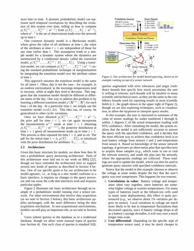
Figure 2:Our architecture for model-based querying, shown as anexample running on top of a sensor network.

queries augmented with error tolerances and target confi-dence bounds that specify how much uncertainty the useris willing to tolerate; such bounds will be intuitive to manyscientific and technical users, as they are the same as the con-fidence bounds used for reporting results in most scientificfields (c.f., the graph shown in the upper right of Figure 2),though we are also exploring techniques, such as visualiza-tion, to allow the layperson to interpret query results.

In this example, the user is interested in estimates of thevalue of sensor readings for nodes numbered 1 through 8,within .1 degrees C of the actual temperature reading with95% confidence. After consulting the model, the system re-alizes that the model is not sufficiently accurate to answerthe query with the specified confidence, and it decides thatthe most efficient way to achieve that confidence level is toread battery voltage from sensors 1 and 2 and temperaturefrom sensor 4. Based on knowledge of the sensor networktopology, it generates anobservation planthat specifies howto acquire those samples (e.g., which route to use to visitthe relevant sensors), and sends the plan into the network,where the appropriate readings are collected. These read-ings are used to update the model, which can then be used togenerate query answers with specified confidence intervals.

Notice that the model in this example chooses to observethe voltage at some nodes despite the fact that the user’squery was over temperature. This happens for two reasons:

1. Correlations in value: Battery voltage and temper-ature often vary together, since batteries are some-what higher voltage at warmer temperatures. For manytypes of batteries (such at the lithium-ion cells usedin many mote deployments), this effect is quite pro-nounced (e.g., we observe about 1% variation per de-gree on motes). Local variations in voltage are muchmore likely to be due to temperature fluctuations thandecreased capacity, since if battery voltage drops at allas a battery’s storage dwindles, it will vary over a muchlonger time scale.

2. Cost differential: Depending on the specific type oftemperature sensor used, it may be much cheaper to

sample the voltage than to read the temperature. Forexample, on sensor boards from Crossbow Corpora-tion for Berkeley Motes [15], the temperature sensorrequires orders of magnitude more energy to samplethan simply reading battery voltage. A primary goal ofour work is to use models to help decide which sensorsare significant and worth acquiring, given differentialdata acquisitional costs and the user’s data demands (asspecified in queries).

Thus, one of the key properties of many probabilistic mod-els is that they can capture correlations between differentattributes.

In general, the software that runs on each of the nodesin the network (shown in the small box on the bottom-leftof Figure 2) includes some code to facilitate model-basedquery execution. Thepredicate checkeris in charge of ap-plying probabilistic predicates to determine if a particularquery answer is worth transmitting – this is needed to helpexecute continuous queries that are looking for outliers orother exceptional conditions. It executes against a local im-age of the model which captures the state and behavior ofthe local node and its relationship to other nodes. Thedatamanagement layeris in charge of managing typed tuples ofdata, which it builds up by calling down into theacquisitionlayer. Note that, in the example described here, the predi-cate checker and local model are not needed, because (in thiscase) the model is stored centrally. In general, centralizedmodels make query planning easier since they have accessto state in a single location, but are more expensive (in termsof communication or energy), because they must collect thatstate to a single location rather storing it locally at the nodes.

There are thus four major steps to query processing in ourarchitecture:

1. Using the model, the query optimizer generates an ob-servation plan which will allow it to answer the queryto within the specified bounds at a minimal cost.

2. The plan is executed by the network, collecting datafrom relevant nodes (and possibly filtering out some re-sults by consulting an in-network version of the model).

3. The model is updated with results collected from thenetwork.

4. Using basic probability computations (Section 2.1), thequery answer and confidence bounds are computed.

We note that he user in Figure 2 could have requested100% confidence and no error tolerance, in which case themodel would have required us to interrogate every sensor.Conversely, the user could have requested very wide confi-dence bounds, in which case the model may have been ableto answer the query without acquiring any additional datafrom the network.

Given this basic introduction to our architecture, we nowturn our attention to some of the ways in which our tech-niques can be applied.

3 ApplicationsSystems that exploit statistical modeling techniques and op-timize the utilization of a network of resource constrained

devices, such as BBQ, could have significant impact in anumber of areas, as outlined by some case studies describedin this section. Although our architecture is targeted pri-marily at acquisitional environments, some of the systemswe discuss do not fall into this category (e.g., database costestimation) and can still benefit from our core probabilisticmodeling technology.

3.1 Sensor applications

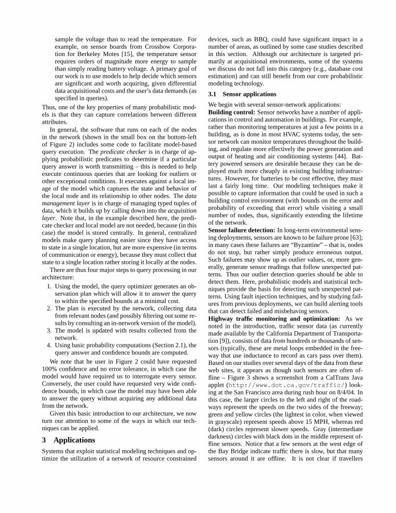
We begin with several sensor-network applications:Building control: Sensor networks have a number of appli-cations in control and automation in buildings. For example,rather than monitoring temperatures at just a few points in abuilding, as is done in most HVAC systems today, the sen-sor network can monitor temperatures throughout the build-ing, and regulate more effectively the power generation andoutput of heating and air conditioning systems [44]. Bat-tery powered sensors are desirable because they can be de-ployed much more cheaply in existing building infrastruc-tures. However, for batteries to be cost effective, they mustlast a fairly long time. Our modeling techniques make itpossible to capture information that could be used in such abuilding control environment (with bounds on the error andprobability of exceeding that error) while visiting a smallnumber of nodes, thus, significantly extending the lifetimeof the network.Sensor failure detection:In long-term environmental sens-ing deployments, sensors are known to be failure prone [63];in many cases these failures are “Byzantine” – that is, nodesdo not stop, but rather simply produce erroneous output.Such failures may show up as outlier values, or, more gen-erally, generate sensor readings that follow unexpected pat-terns. Thus our outlier detection queries should be able todetect them. Here, probabilistic models and statistical tech-niques provide the basis for detecting such unexpected pat-terns. Using fault injection techniques, and by studying fail-ures from previous deployments, we can build alerting toolsthat can detect failed and misbehaving sensors.Highway traffic monitoring and optimization: As wenoted in the introduction, traffic sensor data (as currentlymade available by the California Department of Transporta-tion [9]), consists of data from hundreds or thousands of sen-sors (typically, these are metal loops embedded in the free-way that use inductance to record as cars pass over them).Based on our studies over several days of the data from theseweb sites, it appears as though such sensors are often of-fline – Figure 3 shows a screenshot from a CalTrans Javaapplet (http://www.dot.ca.gov/traffic/ ) look-ing at the San Francisco area during rush hour on 8/4/04. Inthis case, the larger circles to the left and right of the road-ways represent the speeds on the two sides of the freeway;green and yellow circles (the lightest in color, when viewedin grayscale) represent speeds above 15 MPH, whereas red(dark) circles represent slower speeds. Gray (intermediatedarkness) circles with black dots in the middle represent of-fline sensors. Notice that a few sensors at the west edge ofthe Bay Bridge indicate traffic there is slow, but that manysensors around it are offline. It is not clear if travellers

San

Fran

cisc

o Ba

y

East Bay

SanFran

Marin

Figure 3: Screenshot from the California Department of Trans-portation road sensor website in the Bay Area. Green dots rep-resent roads where the traffic is travelling faster than 45 MPH;yellow represents traffic moving 15-45 MPH, and red representstraffic moving at speeds less than 15 MPH. Gray circles with blackdots (added for clarity) represent offline sensors.

should avoid the Bridge, or if this is a localized anomalythat will not cause long delays. Feeding such data to a routeplanning algorithm is likely to cause it to do very strangethings if it tries to apply linear interpolation or other simpletechniques to guess traffic speeds. In contrast, a probabilis-tic model can use data from times when the sensors wereonline, combined with the data from a few of the nodes, toinfer the missing speeds.Structural and factory health monitoring: A popularapplication for sensor networks ispreventative mainte-nance[37], where structures and industrial equipment aremonitored for early signs of failure. A widely used tech-nique for failure detection involves measuring changes inthe phase between vibration signals from groups of sensors– the intuition being that if two parts of a piece of equip-ment are solidly connected, they will vibrate in-phase, butif they suddenly become out-of-phase with each other, thatis a sign that something is wrong. Probabilistic models pro-vide a convenient way to determine the components that areexpected to vibrate in-phase with each other, and outlier de-tection techniques like those used for sensor failure detectioncan identify low-probability changes in the phase structure,indicating the possibility of impending failure.Intrusion detection and tampering: As a part of an in-volvement in MIT’s new Center for Information Securityand Privacy (CISP) [49], we are investigating techniques forintrusion detection in wireless and sensor networks. In sen-sor networks, there are a range of physical attacks that in-volve tampering with devices or sensors. Examples includeintruders seeking to hide information about their presenceor trying to cause a control or regulatory system to misbe-have (e.g., people often ’hack’ computers in their cars to in-crease performance, possibly decreasing safety and increas-

ing emissions). Outlier and influence queries have potentialapplication in detecting this sort of tampering.

3.2 Non-sensor applications

There are also a wide range of non-sensor applications thatcan benefit from our probabilistic model-based approach.Network monitoring: Network monitoring, even in wirednetworks, has the potential to consume a significant propor-tion of available bandwidth. For example, on a typical edgegateway in a large university, per-flow statistics are collectedto identify users and applications that are potential securityconcerns or who are over-utilizing the network. Such statis-tics constitutes tens of MB/sec of data, and, even on a well-provisioned inter-university network, collecting a completeset of such statistics exhausts the CPU and bandwidth capa-bilities of edge routers [40]. Current practice is to randomlysample a subset of flows and store just the sample. Sim-ilarly, in wireless networks, the collection of time-varyinglink quality and congestion information can impose a signif-icant overhead, especially in dynamic networks where suchinformation may change rapidly, requiring frequent link-sampling. We can use probabilistic modeling techniques toestimate and track loss rates, congestion information and se-curity concerns (e.g., types of flows that are likely to useunusual amounts of bandwidth or are otherwise outliers),exploiting correlations to avoid acquiring data that can beinferred from a well-chosen subset of available readings.Database summaries:Capturing the joint data distributionof multi-dimensional data sets through compact and accu-ratesynopsesis a fundamental problem arising in a variety ofpractical scenarios, includingquery optimization, query pro-filing, andapproximate query answering. Cost-based queryoptimizers employ such synopses to obtain accurate esti-mates of intermediate result sizes that are, in turn, needed toevaluate the quality of different execution plans. Similarly,query profilers and approximate query processors requirecompact data synopses in order to provide users with fast,useful feedback on their original query [11, 59]. Such queryfeedback (typically, in the form of anapproximate answer)allows OLAP and data-mining users to identify the truly in-teresting regions of a data set and, thus, focus their explo-rations quickly and effectively, without consuming inordi-nate amounts of valuable system resources. Further, userscan make informed decisions on whether they would liketo invest more time and resources to fully executing theirqueries.

The idea of using probabilistic modeling techniques tobuild synopses has already been explored [18, 27]. As thisprevious work shows, using probabilistic models to captureand exploit the correlations in the data can lead to signifi-cantly more compact summaries. The techniques we havedeveloped can be directly applied in this context as well;in particular we are interested in answering more complexqueries as well as in providing probabilistic guarantees tothe user.Load shedding in streams:Load-shedding is cited as a re-quirement in many stream-based query processors [52, 10].The Aurora [10] project proposessemantic load shedding,

where input tuples that correspond to particular output val-ues are considered more important than other tuples (andare thus not shed). The authors of Aurora propose a schemewhere the query plan is “reversed” to determine such input-output mappings, but for general query plans, such an ap-proach is infeasible, since operations like joins and aggre-gates are not readily invertible. As a more tractable alter-native, we can use probabilistic models to determine the re-lationship between inputs and outputs, keeping input tuplesthat have a high probability of mapping to valued outputs.These probabilistic relationships may include correlationsbetween different fields in the input tuples, so that, for ex-ample, the model may determine that intermediate join tu-ples have a low probability of producing a high-value out-put, even though the base tuples of the join both had a highvalue prior to the join.Monitoring distributed streams: Recently there has alsobeen an increasing interest in distributed data streams,i.e.,data streams that originate and are processed in a distributedfashion [23, 13]. Though similar to sensor networks inmany aspects, the optimization goal in such systems is net-work latency, not the battery life of the sensors. The IrisNetproject [23] proposes use of caching to reduce the latenciesincurred in query answering. We believe a model-based ap-proach can lead to both better answer quality, and a reduc-tion in latencies, especially in applications such as the moti-vatingparking space finderapplication of IrisNet.

4 New queriesThese applications require a range of new queries that non-probabilistic database systems are ill-equipped to answer. Inthis section, we summarize the range of new queries that weare working to support.Probabilistic, approximate queries: The most basic classof queries that we anticipate users to ask are probabilisticand approximate variations of traditional SQL queries. Ex-amples of such queries include queries asking fortemper-ature at a certain location in a building, oraverage speedalong a segment of a highway. We can support such queriesby using additional predicates in SQL expressions that spec-ify the confidence that the user wants in the answer, or theerror she is willing to tolerate. This class of queries coverstraditionalexactqueries which can be asked by setting theconfidence required to 100%.

Our initial effort in BBQ provided support for this typeof query; Figure 4 shows one advantage of approximatequeries: improved performance. In this case, we ran threerange queries over temperature readings from a 11 nodesensor deployment in the Berkeley Botanical Garden. Wetrained our model for 20 days and ran test queries over a 10day period. We used pre-collected data so we could verifythe accuracy of our approximate query answers during thistest period. If we had asked an exact query, we would havebeen required to observe the value of every sensor at eachpoint in time; using our Gaussian-based probabilistic modelwith queries specifying 95% confidence, we were requiredto observe the values of only a small fraction of the sensors.The truth values of the predicates on the unobserved sensors

could be accurately predicted by exploiting cross-sensor cor-relations (in all cases, we had less than the 5% allowed er-rors when we compared the predicted predicate values to theactual values from the test data). Notice that different pred-icates require observation of different numbers of sensors atdifferent times of day – this is because of the natural tem-perature distributions in the garden that our model is able toexploit. For example, during the day, the temperatures aretypically significantly higher than the top end of the rangespecified in first predicate (16-17 degrees). Because of this,during the day, very few observations need to be made to as-certain that the predicate is false with sufficient confidence.

0

20

40

60

80

100

6:00 12:00 18:00 0:00 6:00 12:00 18:00 0:00

Time of Day

Per

cent

age

of O

bser

ved

Nod

es

Range [16-17]Range [19-20]Range [21-22]

Figure 4:Percentage of observed sensors versus time of day for a36 hour period over 11 sensors deployed in the Berkeley BotanicalGarden for three different range predicate queries. In this case, wesetδ = 5% (95% confidence).

Outlier queries: Outliers are essentially events of low prob-ability, and use of probabilistic models provides an excel-lent mechanism to detect outliers. To detect outliers, theuser could ask the system to report whenever any attributevalue occurs that has a low user-specified probability of oc-currence, or that differs from its expected value by morethan some threshold. As an example, a user might registera continuous query that reports any time the bandwidth ontheir wireless network is more than three times the expectedvalue for the current time of day. Note that, outlier detectionwill typically require continuous observation of the underly-ing attributes at the motes, and the main advantage of usingmodels in this case would be to save communication cost(though knowledge of how often, and under what circum-stances outliers are expected to occur may be used to reducethe observation costs as well).Prediction queries: These queries estimate the value of anattribute or predicate either (1) at a location where there arecurrently no available devices, or (2) at some time in nearfuture, with the best precision (and report that precision andconfidence in the estimate). For example, a user might ask:“What will the temperature in Room 938 be in 10 minutes?”Similarly, users might post “what-if” queries, to discoverhow a change in one attribute might affect other attributes– for example, in a system monitoring application, a usermight ask how increasing bandwidth on a given link wouldincrease CPU utilization on a given processor.Queries over hidden variables: In many scenarios, there

may be interesting variables that cannot be directly ob-served, but that can be reasoned about. For example, ina sensor network that has sensors for monitoringtempera-ture, pressureandlight, but not for monitoringrain, we cannever “observe” rain directly, but it may be possible to inferwhether it is raining or not based on the values of the observ-able variables. There has been much work on hypothesizingabout hidden variables (in the above example, we knew be-forehand about existence of an unobservable variable; theremay be cases where we have first infer that a hidden variableexists), and learning structures containing them [25]. We ex-pect to be able to leverage these existing techniques in ourwork.Influence queries: Use of probabilistic models also opensup avenues for asking sophisticated analysis queries. Onesuch class of queries areinfluence queries, where the usermight want to know which attributes are most closely cor-related with the value of a particular attribute. Such queriescan be used to help infer causality or determine when sen-sors in an area are redundant. For example, a user mightask the question: “What percentage of the traffic on linki ispredicted by the traffic on linksj andk over all time?”

5 ChallengesGiven these applications and queries, we now discuss someof the challenges they present, followed by a set of tech-niques we are exploring to address these challenges.Model selection: Choosing the best model for the givenquery workload and environment is a key issue. The choiceof model affects many aspects of our approach:

• Accuracy of the answers:Recall that we provide prob-abilistic answers to the user, and the confidence in theanswers provided relies on the assumption that the un-derlying data follows the model with sufficient accu-racy. If this is not the case, the answers provided byour models could be erroneous.

• Ability to answer certain types of queries:Some mod-els are more naturally suited to answer certain typesof queries. For example, outlier detection requires thesystem to continuously sample sensors and check themagainst the model to see if they have a low probabilityof occurring. To do this efficiently, we may require amodel that is distributed across the nodes in a system.

• Algorithmic aspects of querying:The techniques toquery the model efficiently are highly dependent on thechoice of the model. The space and time requirementsof different models can vary by orders of magnitude.

Selecting a suitable model for the data is one of the criticalchallenges in the deployment of model-based systems.Transparency in model selection and usage:Althoughdifferent models may be better suited for different environ-ments and for different classes of queries, developing a com-pletely new system for each different model may be a wasteof time and development effort. Ideally, using a new modelshould involve little to no effort on the part of user. Given alarge variety of models that may be applicable in various dif-ferent scenarios, this may turn out to be a tremendous chal-

lenge.Data acquisition: Irrespective of the model selected, whenand how to acquire data is one of the key issues that needsto be addressed. In most of the scenarios that we envisiona model-based system being deployed, the cost of acquiringand/or transferring data is the dominant cost. For example,in sensor networks, both the cost of sampling data, and thecost of communicating it to the basestation are high – for ex-ample, in a recent analytical study, we estimated that 98% ofenergy in a typical sensor network data collection scenariowas consumed sampling sensors or communicating. In dis-tributed system where the data is being generated all overthe world, minimizing thelatency in answering the querycould be the optimization goal. There are two aspects to thisproblem:

• When to acquire data: This is partly dependent onthe model and the user query. To maintain the re-quired confidence in the answers it provides, the modelcould ask for more samples of the underlying data. Inmany cases, we expect that the same confidence maybe achieved in many different ways,i.e., by samplingdifferent sets of attributes of the data. Because of this,the question ofwhento acquire data will typically betightly integrated with the question ofhow it is ac-quired.

• How to acquire data: Most of the environments wehave discussed so far exhibit highly non-uniform coststructures. For example, in sensor networks, the costsof sampling different attributes can be wildly different.Also, the multi-hop nature of communication in sen-sor networks means that sampling sensors closer to thebase station is cheaper than sampling far away sensors.

Issues surrounding when and how data is collected areamongst of the most interesting algorithmic challenges inthe development and deployment of model-based systems.Training and retraining: In general, a probabilistic modelis only as good at prediction as the data used to train it. Formodels to perform accurate predictions they must be trainedin the kind of environment where they will be used. Thatdoes not mean, however, that well-trained models cannotdeal with changing relationships over time; for example, themodel we used in BBQ[21] uses different correlation datadepending on time of day. Extending it to handle seasonalvariations, for example, is a straightforward extension of thetechniques we use for handling variations across hours of theday. Typically in probabilistic modeling, we pick a class ofmodels, and use learning techniques to pick the best modelin the class. The problem of selecting the right model classhas been widely studied (e.g., [50]), but can be difficult insome applications.

In Section 6, we outline a more general Bayesian ap-proach that integrates querying of the data with learning.Data model and query language:Our initial efforts havefocused on building simple Gaussian models and demon-strating that they can answer certain classes of queries [21].However, we do not have an integrated acquisition-orienteddatabase system that includes notions of uncertainty or mod-

eling, and it is not clear how such models can be integratedin a general way into the existing relational data model andquery languages. One possible data representation is to at-tach a probability distribution to each data point – severalproposals for probabilistic data models of this type havebeen made in the literature [42, 3, 24, 27], and we may beable to adapt this existing work. None of these approaches,however, focus on the data acquisition or model-learning is-sues. Instead, they concentrate representing user-specifieduncertainty in the database; the approaches do not help usaddress our principal challenge of acquiring appropriate datato answer user queries at the desired confidences.

As an initial step towards supporting uncertainty in ourquery language, we currently representε, δ bounds as addi-tional query predicates in SQL expressions, as in the queryshown in Figure 2 above, but there are a number of outstand-ing questions about how a system deals with readings withdiffering levels of uncertainty. For example, how can read-ings with different uncertainties from different sub-queriesbe composed into a final query result? What should we doif our models cannot answer queries to a given confidencelevel? Are there other representations besides confidencethat we should consider (e.g., absolute or relative deltas)?

Exposing uncertainty to the user: One issue with expos-ing uncertainty to the user is that it requires him or her tounderstand the basics of probability. Although this may beacceptable for scientific users who are used to statistical testsof significance and other confidence metrics, for the lay-person, such notions will be quite confusing. One possi-bility is to convert probabilistic answers to definite answerswhen result confidence is above a give threshold, suppress-ing the uncertainty report. Though at first this appears to beno better than what traditional uncertainty-unaware databasedo, it is in fact substantially better as the user is never ex-posed to answers that do not have a high probability of be-ing true. For example, in the case of the California Freewaysensors given in the introduction, users wouldn’t receive av-erage speeds for segments where the uncertainty was low,preventing them from inadvertently using congested routes.

The other possibility we are exploring is to avoid theseconcerns through the use of visualization tools. Figure 5shows a visualization mockup of uncertainty in readingsfrom a single sensor. It shows a stream of temperature read-ings from a single sensor; the small circles represent pointsof time when readings are actually captured. The contoursrepresent different levels of uncertainty in readings. Thedarkest, narrowest band corresponds to a band of confidenceabout the most probable value of the sensor – in this case,there is a 90% chance the true value of the sensor is inthis band. The lighter, outermost band captures the rangeof readings where the true value lies with 99% probability.This visualization could be built using a probabilistic modelsuch as our Gaussian model and provides an intuitive repre-sentation of uncertainty.

Figure 6 shows a second visualization of uncertainty in-formation for a query that collects readings from a set ofgeographically distributed sensors (in this case, sensors are

Time12:05:30 2:05:30

Temperature

99%

90%95%

Figure 5: Mockup visualization of a display used to visualize un-certainty in a stream of readings coming from a sensor.

X

Y

15°C

25°C

Figure 6: Mockup visualization of uncertainty display of a set oftemperature sensors (circles outlined in black) on Nantucket Is-land. Confidence in readings is represented by colored-dot density.

shown on a portion of Nantucket Island). In this case, colorsrepresent temperature estimates; large solid circles representthe locations of sensors. White circles are inactive sensorsthat were not involved in data collection. Densely coloredregions represent areas where there is high certainty on thereading, with sparsely colored regions having low certainty.These certainties can be derived, for example, from a proba-bilistic model that represents correlations between the activesensors and the inactive sensors. Such a visualization al-lows users to quickly determine where more sensors may beneeded, and to understand how well sensors are monitoringan area of interest.

We are planning to build support for both types of uncer-tainty visualization into our system.

Continuous vs. snapshot queries:We plan to supportboth snapshot queries,i.e., one-time queries about the cur-rent state of the system, and continuous queries,i.e., querieswhich the user wants to know the answers of on a peri-odic basis. Depending on the optimization goals, these twoclasses of queries pose different optimization challenges.The challenge with snapshot queries is to balance “push”vs “pull”. Pushing too much data towards the user can leadto wasted communication; on the other hand, having the sys-tem pull data for every snapshot query could lead to unrea-sonable latencies. For a continuous query, we must figureout which nodes should stay active, when to do samplingand how to communicate the data from those nodes to thebase station. Though it is possible to optimize the data ac-quisition process heavily, dynamic sensornet topologies can

SERVER

LAB

KITCHEN

COPYELEC

PHONEQUIET

STORAGE

CONFERENCE

OFFICEOFFICE50

51

52 53

54

46

48

49

47

43

45

44

42 41

3739

38 36

33

3

6

10

11

12

13 14

1516

17

19

2021

22

242526283032

31

2729

23

18

9

8

7

4

34

1

2

3540

Figure 7:Structure of graphical model learned for the temperaturevariables for a deployment in the Intel Berkeley Lab [56].

complicate matters.

6 New techniquesIn order to address the wide range of applications and newqueries described in Sections 3 and 4, and to surmount thechallenges in Section 5, it is insufficient to simply adaptexisting methods in data bases, machine learning and dis-tributed systems; we need new integrated approaches. Thissection outlines techniques that can address some of theseissues as well as research directions that we are currentlypursuing.

6.1 Representations for probability distributions

Probabilistic models are the centerpiece of our approach. InSection 2.1, we described very general probability distribu-tions,p(X1, X2, . . . , Xn). Choosing the appropriate repre-sentation for such distribution, allowing us to represent com-plex correlations compactly, to learn the parameters effec-tively, and to answer queries efficiently is one of the biggestchallenges in this research. Probabilistic graphical modelsare a very appropriate choice to address these issues [57].

In a (probabilistic) graphical model, each node is associ-ated with a random variable. Edges in the graph represent“direct correlation”, or, more formally, conditional indepen-dencies in the probability distribution. Consider, for exam-ple, the sensor deployment shown in Figure 7, where theattributes are the temperatures in various locations in the In-tel Berkeley Lab. The graphical model in Figure 7 assumes,for instance, that temperatures in the right side of the lab areindependent of those in the left side, given temperatures inthe center (e.g., T20 andT47 are independent givenT10, T32,andT33).

The sparsity in graphical models is the key to effi-cient representation and probabilistic querying [14]. Indiscrete settings, for example, a naive representation ofp(X1, X2, . . . , Xn) is exponential in the number of at-tributesn, while a graphical model is linear inn and, in theworst case, exponential in the degree of each node. In addi-tion to reducing space complexity, reducing the number ofparameters can prevent overfitting when the model is learnedfrom small data sets. Similarly, answering a query naively isexponential inn, while in a graphical model the complexityis linear inn and exponential in the tree-width of the graph.

In our setting, in addition to allowing us to answer queriesefficiently, graphical models are associated with a widerange of learning algorithms [34]. These algorithms can be

0 0.2 0.4 0.6 0.8 10

0.2

0.4

0.6

0.8

1

Beta(1,1)

parameter value

Beta

pdf

0 0.2 0.4 0.6 0.8 10

0.2

0.4

0.6

0.8

1

1.2

1.4

1.6Beta(2,2)

parameter value

Beta

pdf

(a) (b)

0 0.2 0.4 0.6 0.8 10

0.5

1

1.5

Beta(3,2)

parameter value

Beta

pdf

0 0.2 0.4 0.6 0.8 10

1

2

3

4

5

6Beta(30,20)

parameter value

Beta

pdf

(c) (d)Figure 8:Bayesian approach for learning the parameter of a coin:(a) prior distribution, Beta(1,1); posterior distributions over thecoin parameter after observing: (b) 1 head, 1 tail; (b) 2 heads, 1tail; (b) 29 heads, 19 tails.

used both for learning a model from data, and to evaluatethe current model, addressing many of the model selectionissues discussed above.

Additionally, graphical models allow us to efficiently ad-dress hidden variables, both in terms of answering queriesand of learning about hidden variables [25]. In the examplein Figure 7, each node could be associated with a faulty sen-sor hidden variable [43]. When a node is faulty, the sensedvalue is, for example, independent of the true temperature.By exploiting correlations in the temperatures measured bythe nodes and sparsity in the graphical model, we can effi-ciently answer outlier queries.

Finally, there is vast graphical models literature for ad-dressing other types of queries and models. For example,these models can be extended to allow for efficient repre-sentation and inference in dynamical systems [8, 17], and toanswer causal queries [58].

6.2 Integrating learning and querying

Thus far, we have focused on a two-phase approach: in thefirst phase, we learn the probabilistic model, and in the sec-ond, we use the model to answer queries. This is an artificialdistinction, raising many questions, such as when should westop learning and start answering queries. We can addressthis issue by applying aBayesian learningapproach [6].

In a Bayesian approach, we start with aprior distributionp(Θ) over the model parametersΘ. After observing somevalue for the attributesx, we use Bayes rule to obtain apos-terior distributionover the model parametersp(Θ | x):

p(Θ | x) ∝ p(x | Θ)p(Θ). (1)

This process is repeated as new data is observed, updatingthe distribution over model parameters.

Consider, for example, the task of learning the parame-ter of a biased coin; that is, the coin flips are independentlydistributed according to the usual binomial distribution withunknown parameter. Typically, for efficiency reasons, we

choose a prior distribution that yields a closed form repre-sentation of the posterior in Equation (1); when such closed-form solutions are possible, the priorp(Θ) and the likeli-hood functionp(x | Θ) are said to beconjugate. In ourexample, Beta distributions are conjugate to the binomialdistribution of the coin. Figure 8 illustrates the process ofBayesian learning for our coin example: We start with theBeta(1,1) in Figure 8(a); here, the distribution over possiblecoin parameters is almost uniform. Figures 8(b)-(d) illus-trate the posterior distribution over the coin parameters aftersuccessive observations. As more coin flips are observed,the distribution becomes more peaked. Thus, when answer-ing a query about the coin after a few flips, our answer willbe uncertain, but after making a larger number of observa-tions, the answer will have significantly lower variance.

These ideas can be integrated with our approach to avoidthe need for a separate learning phase. Consider the Gaus-sian distributions used in the BBQ system. Initially, we maybe very uncertain about the mean and covariance matrix ofthis distribution, which can be represented by a highly un-certain prior (the conjugate prior for the covariance matrixis the Wishart distribution). Thus, when faced with a query,we will need to observe the value of many sensors. How-ever, using Bayesian updating, after we observe these sensorvalues, in addition to answering the query at hand, we be-come more certain about the mean and covariance matrix ofthe model. Eventually, we will be certain about the modelparameters, and the number of sensors that we will needto observe will automatically decrease. This integrated ap-proach achieves two goals: first, the learning phase is com-pletely eliminated; second, using simple extensions, we canadd dynamics to the parameter values, allowing the modelto change over time.

6.3 Long-term query plans

Modeling the correlations between different attributes in thesystem and also, the correlations across time, enables thequery planner to consider a much richer class of executionplans than previously possible.

One such interesting class of execution plans that we haveexplored in our previous work [20] areconditional plans.These plans exploit the correlations present in the data byintroducing low-cost predicates in the query execution planthat are used to change the ordering of the more expensivepredicates in the query plan.

As an example, consider a query containing two predi-catestemp > 20o C, and light < 100 Lux over asensor network. Let theapriori selectivities of these twopredicates be1

2 and 12 respectively, and let the costs of

acquiring the attributes be equal to 1 unit each. In thatcase, either of the two plans a traditional query processormight choose has expected cost equal to 1.5 units (Figure9). However, we might observe that the selectivities of thesetwo predicates vary considerably depending on whether thequery is being evaluated during the day or at night. For in-stance, in Berkeley, during Summer, the predicate ontempis very likely to be false during the night, whereas the pred-icate onlight is very likely to be false during the day.

Light < 100 Lux

Temp > 20° C

Temp > 20°C

Light < 100 Lux

Traditional Plans

Light < 100 Lux

Temp > 20° C

Temp > 20°C

Light < 100 Lux

Time in [6am, 6pm]

T

F

A Conditional Plan

SELECT * FROM sensorsWHERE light < 100 Lux AND temp > 20° C

Figure 9:A conditional query plan that uses different ordering ofquery predicates depending on the time of day.

This observation can be utilized to construct aconditionalplan as shown in the figure that checks the time of the dayfirst, and evaluates the two query predicates in different or-der depending on the time. Assuming that the selectivity ofthe temp predicate is1

10 at night, and the selectivity of thelight predicate is1

10 during day, the expected cost of thisplan will be 1.1 units, a savings of almost 40%.

More generally, in continuous queries, additional costsavings can be obtained by exploiting similarities betweenqueries. For example, if we know that the next query willrequire an attribute at a particular nodei, and the currentquery plan observes values at nearby nodes, then it is proba-bly better to visit nodei as well in the current time step.

The optimal solution to such long-term planning prob-lems can be formulated as aMarkov decision process(MDP) [5, 60]. In an MDP, at each time step, we observethe current state of the system (in our setting, the currentdistribution and query), and choose an action (our observa-tion plan); the next state is then chosen stochastically giventhe current state (our next query and distribution). Unfor-tunately, traditional approaches for solving MDPs are expo-nential in the number of attributes. Recently, new approx-imate approaches have been developed to solve very largeMDPs by exploiting structure in problems represented bygraphical models [7, 32]. Such approaches could be ex-tended to address the long-term planning problem that arisesin our setting.

6.4 In-network processing

Thus far, we have focused on algorithms where the proba-bilistic querying task occurs in a centralized fashion, and weseek to find efficient network traversal and data gatheringtechniques. However, in typical distributed systems, nodesalso have computing capabilities. In such settings, we canobtain significant performance gains by pushing some of theprocessing into the network.

In some settings, we can reduce communication by ag-gregating information retrieved from the network [45, 35].We could integrate these techniques with our models by con-ditioning on the value of the aggregate attributes rather thanthe sensor values. Such methods will, of course, increase ourplanning space: in addition to finding a path in the networkfor collecting the required sensor values, we must decidewhether to aggregate values along the way.

More recently, a suite of efficient algorithms has been de-veloped for robustly solving inference tasks in a distributedfashion [31, 56]. In these approaches, each node in thenetwork obtains a local view of a global quantity. For ex-

ample, each node computes the posterior probability over asubset of the attributes given the sensor measurements at allnodes [56]; or each node obtains a functional representation(e.g., a curve fit) of the sensor (e.g., temperature) field [31].Given such distributed algorithms, we can push some ofthe probabilistic query processing into the network, allow-ing nodes to locally decide when to make observations andwhen to communicate. When integrated with a system likeBBQ, these methods allow the user to connect to any nodein the network, which can collaborate with the rest of thenetwork to answer queries or detect faulty nodes.

7 Related workThere have been other model-based approaches for queryanswering that rely on a model-like abstraction [64, 55, 54,39]. In most cases, the related work assumes a client-serverrelationship, where the model runs on the server and moni-tors the value of a number of attributes at the clients. Theseapproaches maintain a bound or trajectory over each of theattribute values at the server, using that bound to predict thevalue. When the clients notice that their value no longerfits the model, or when the server has sufficient bandwidthor energy, it will directly observe the attribute values andupdate the model. Our approach differs from previous re-search in that it uses multidimensional probabilistic modelsthat track the relationship between attributes in addition tothe values of attributes themselves. These relationships, orcorrelations, allow the model to update its value estimates ofmany attributes when a single attribute is observed; modelscan be built across attributes that are directly observed (e.g.,light readings from sensors), as well as global attributes(e.g., time of day), and derived attributes (e.g., network lossrate).

There has been substantial work on approximate queryprocessing in the database community, often using model-like synopsesfor query answering much as we rely on proba-bilistic models. For example, the AQUA project [30, 28, 29]proposes a number of sampling-based synopses that can pro-vide approximate answers to a variety of queries using afraction of the total data in a database. As in our approach,such answers typically include tight bounds on the correct-ness of answers. AQUA does not exploit correlations. A fewrecent papers [18, 27] propose exploiting data correlationsthrough use of graphical model techniques for approximatequery processing, but neither provide any guarantees on theanswers returned. Recently, Considineet al. [41] and Gib-bonset al. [53] have shown that sketch based approximationtechniques can be applied in sensor networks to compute ag-gregates. Others have proposed approximation techniquesfor stream-query processing,e.g., Daset al. [16] and Mot-waniet al. [51].

Approximate and best effort caches [55, 54], as well assystems for online-aggregation [61] and stream query pro-cessing [52, 10, 12] include some notion of answer qualityand include the ability to discard some tuples. Most relatedwork focuses on quality with respect to summaries, aggre-gates, or staleness of individual objects already stored in thesystem, as opposed to readings being actively acquired by

the query processor.Several proposals for probabilistic data models have been

made in the literature. For example, ProbView[42] providesa data model based on discrete pdfs, and shows how to an-swer a number of queries in such a domain. Getoor [26] ex-plores a number of probabilistic extensions to the relationalmodel, and shows how statistical models can be learnedfrom relations. Barbaraet al. [3] present some initial re-sults on probabilistic data models. Faradjianet al. [24]present a data model based on continuous pdfs. None ofthese approaches focus on the data acquisition issues, butrather on representing uncertainty in the database, and ontypes of query processing that can be applied to probabilis-tic attributes.

The probabilistic modeling techniques we describe arebased on standard results in machine learning and statistics(e.g., [62, 50, 14]). There are also a number of proposedtechniques for outlier detection [4, 1, 2]. We believe, how-ever, that our approach is one of the first architectures thatcombines model-based approximate query answering withquery processing and optimization and an uncertainty-awaredata model and query language.

8 ConclusionsThe integration of database systems with probabilistic mod-eling will enable database systems to tolerate loss, detectfaulty or erroneous inputs, and identify correlations that canbe used to improve query performance while enabling arange of new types of queries. Such models are particu-larly useful in acquisitional settings such as sensornets andInternet monitoring where the data acquisition costs are typ-ically very high; even for non-acquisitional applications, be-ing able to deal with noisy and lossy data in a seamlessmanner, and the ability to model and reason about data cor-relations can prove to be tremendously useful. There area number of architectural and algorithmic challenges asso-ciated with fully integrating these techniques into databasesystems and, although we believe we have taken some ini-tial steps towards this end, we look forward to many yearsof fruitful cross-disciplinary research. We envision this re-search leading to significant improvements in the utility andefficiency of database systems at managing real-world data.

References[1] C. C. Aggarwal and P. S. Yu. Outlier detection for high dimensional

data. InProceedings of SIGMOD, pages 37–46, 2001.[2] A. Arning, R. Agrawal, and P. Raghavan. A linear method for devia-

tion detection in large databases. InProceedings of KDD, 1995.[3] D. Barbara, H. Garcia-Molina, and D. Porter. The management of

probabilistic data.IEEE TKDE, 4(5):487–502, 1992.[4] V. Barnett and T. Lewis.Outliers in Statistical Data. John Wiley and

Sons, New York, 1994.[5] R. E. Bellman.Dynamic Programming. Princeton, 1957.[6] J. Bernardo and A. Smith.BAYESIAN THEORY. Wiley, 1994.[7] C. Boutilier, R. Dearden, and M. Goldszmidt. Exploiting structure in

policy construction. InProc. IJCAI, pages 1104–1111, 1995.[8] X. Boyen and D. Koller. Tractable inference for complex stochastic

processes. InProc. UAI, 1998.[9] California Department of Transportation. Caltrans realtime freeway

speed map. Web Site.http://www.dot.ca.gov/traffic/ .[10] D. Carney, U. Centiemel, M. Cherniak, C. Convey, S. Lee, G. Seid-

man, M. Stonebraker, N. Tatbul, and S. Zdonik. Monitoring streams- a new class of data management applications. InVLDB, 2002.

[11] K. Chakrabarti, M. N. Garofalakis, R. Rastogi, and K. Shim. Approx-imate query processing using wavelets. InVLDB 2000, Proceedingsof 26th International Conference on Very Large Data Bases, Septem-ber 10-14, 2000, Cairo, Egypt, pages 111–122, 2000.

[12] S. Chandrasekaran, O. Cooper, A. Deshpande, M. J. Franklin, J. M.Hellerstein, W. Hong, S. Krishnamurthy, S. R. Madden, V. Raman,F. Reiss, and M. A. Shah. TelegraphCQ: Continuous dataflow pro-cessing for an uncertain world. InCIDR, 2003.

[13] O. Cooper, A. Edakkunni, M. Franklin, W. Hong, S. Jeffery, S. Krish-namurthy, F. Reiss, S. Rizvi, and E. Wu. Hifi: A unified architecturefor high fan-in systems. InVLDB, 2004.

[14] R. Cowell, P. Dawid, S. Lauritzen, and D. Spiegelhalter.ProbabilisticNetworks and Expert Systems. Spinger, New York, 1999.

[15] I. Crossbow. Wireless sensor networks (mica motes).http://www.xbow.com/Products/Wireless_Sensor_Networks.htm .

[16] A. Das, J. Gehrke, and M. Riedewald. Approximate join processingover data streams. InProceedings of SIGMOD, 2003.

[17] T. Dean and K. Kanazawa. A model for reasoning about persistenceand causation.Computational Intelligence, 5(3):142–150, 1989.

[18] A. Deshpande, M. Garofalakis, and R. Rastogi. Indepen-dence is Good: Dependency-Based Histogram Synopses for High-Dimensional Data. InProceedings of SIGMOD, May 2001.

[19] A. Deshpande, C. Guestrin, W. Hong, and S. Madden. Intel labdata. Web Page.http://berkeley.intel-research.net/labdata .

[20] A. Deshpande, C. Guestrin, W. Hong, and S. Madden. Exploitingcorrelated attributes in acquisitional query processing. InICDE, 2005.

[21] A. Deshpande, C. Guestrin, S. Madden, J. Hellerstein, and W. Hong.Model-driven data acquisition in sensor networks. InVLDB, 2004.

[22] A. Deshpande, C. Guestrin, S. Madden, J. M. Hellerstein, andW. Hong. Model-driven data acquisition in sensor networks. InVLDB, 2004.

[23] A. Deshpande, S. Nath, P. Gibbons, and S. Seshan. Cache-and-queryfor wide area sensor databases. InProceedings of SIGMOD, 2003.

[24] A. Faradjian, J. Gehrke, and P. Bonnet. GADT: A Probability SpaceADT For Representing and Querying the Physical World. InICDE,2002.

[25] N. Friedman. Learning belief networks in the presence of missingvalues and hidden variables. InProc. 14th International Conferenceon Machine Learning, pages 125–133, 1997.

[26] L. Getoor. Learning Statistical Models from Relational Data. PhDthesis, Stanford University, 2001.

[27] L. Getoor, B. Taskar, and D. Koller. Selectivity estimation using prob-abilistic models. InProceedings of SIGMOD, May 2001.

[28] P. B. Gibbons. Distinct sampling for highly-accurate answers to dis-tinct values queries and event reports. InProc. of VLDB, Sept 2001.

[29] P. B. Gibbons and M. Garofalakis. Approximate query processing:Taming the terabytes (tutorial), September 2001.

[30] P. B. Gibbons and Y. Matias. New sampling-based summary statisticsfor improving approximate query answers. InSIGMOD, 1998.

[31] C. Guestrin, P. Bodik, R. Thibaux, M. Paskin, and S. Madden. Dis-tributed regression: an efficient framework for modeling sensor net-work data. InProceedings of IPSN, 2004.

[32] C. E. Guestrin, D. Koller, and R. Parr. Multiagent planning with fac-tored MDPs. In14th Neural Information Processing Systems (NIPS-14), pages 1523–1530, Vancouver, Canada, December 2001.

[33] D. Hand, H. Mannila, and P. Smyth.Principles of Data Mining. MITPress, 2001.

[34] D. Heckerman. A tutorial on learning with bayesian networks, 1995.[35] J. Hellerstein, W. Hong, S. Madden, and K. Stanek. Beyond aver-

age: Towards sophisticated sensing with queries. InProceedings ofthe First Workshop on Information Processing in Sensor Networks(IPSN), March 2003.

[36] J. M. Hellerstein, M. J. Franklin, S. Chandrasekaran, A. Deshpande,K. Hildrum, S. Madden, V. Raman, and M. Shah. Adaptive query pro-cessing: Technology in evolution.IEEE Data Engineering Bulletin,23(2):7–18, 2000.

[37] Intel Research. Exploratory research - deep networking. WebSite. http://www.intel.com/research/exploratory/heterogeneous.htm#preventativ%emaintenance .

[38] Z. G. Ives, D. Florescu, M. Friedman, A. Levy, and D. S. Weld. An

adaptive query execution system for data integration. InProceedingsof SIGMOD, 1999.

[39] A. Jain, E. Change, and Y.-F. Wang. Adaptive stream resource man-agement using kalman filters. InProceedings of SIGMOD, 2004.

[40] Jim Madden, Director UCSD Network Operations. Personal commu-nication, July 2004.

[41] G. Kollios, J. Considine, F. Li, and J. Byers. Approximate aggregationtechniques for sensor databases. InICDE, 2004.

[42] L. V. S. Lakshmanan, N. Leone, R. Ross, and V. S. Subrahmanian.Probview: a flexible probabilistic database system.ACM TODS,22(3):419–469, 1997.

[43] U. Lerner, B. Moses, M. Scott, S. McIlraith, and D. Koller. Monitor-ing a complex physical system using a hybrid dynamic bayes net. InUAI, 2002.

[44] C. Lin, C. Federspiel, and D. Auslander. Multi-Sensor Single Actu-ator Control of HVAC Systems. InInternation Conference for En-hanced Building Operations, 2002.

[45] S. Madden.The Design and Evaluation of a Query Processing Archi-tecture for Sensor Networks. PhD thesis, UC Berkeley, 2003.

[46] S. Madden, M. J. Franklin, J. M. Hellerstein, and W. Hong. Thedesign of an acquisitional query processor for sensor networks. InProceedings of SIGMOD, 2003. To Appear.

[47] S. Madden, W. Hong, J. M. Hellerstein, and M. Franklin. TinyDB webpage.http://telegraph.cs.berkeley.edu/tinydb .

[48] A. Mainwaring, J. Polastre, R. Szewczyk, and D. Culler. Wirelesssensor networks for habitat monitoring. InACM Workshop on SensorNetworks and Applications, 2002.

[49] MIT CSAIL Center for Information Security and Privacy. Home page.http://csg.lcs.mit.edu/CISP/ .

[50] T. Mitchell. Machine Learning. McGraw Hill, 1997.[51] R. Motwani, J. Widom, A. Arasu, B. Babcock, S. Babu, M. Datar,

G. Manku, C. Olston, J. Rosenstein, and R. Varma. Query process-ing, resource management, and approximation in a data stream man-agement system. InProceedings of CIDR, 2003.

[52] R. Motwani, J. Window, A. Arasu, B. Babcock, S.Babu, M. Data,C. Olston, J. Rosenstein, and R. Varma. Query processing, approxi-mation and resource management in a data stream management sys-tem. In First Annual Conference on Innovative Database Research(CIDR), 2003.

[53] S. Nath and P. B. Gibbons. Synopsis diffusion for robust aggregationin sensor networks. InProceedings of VLDB, 2004.

[54] C. Olston and J.Widom. Best effort cache sychronization with sourcecooperation. InProceedings of SIGMOD, 2002.

[55] C. Olston, B. T. Loo, and J. Widom. Adaptive precision setting forcached approximate values. InProceedings of SIGMOD, May 2001.

[56] M. A. Paskin and C. E. Guestrin. Robust probabilistic inference indistributed systems. InUAI, 2004. In the20th International Confer-ence on Uncertainty in Artificial Intelligence.

[57] J. Pearl.Probabilistic Reasoning in Intelligent Systems: Networks ofPlausible Inference. Morgan Kaufmann Publishers, 1988.

[58] J. Pearl.Causality : Models, Reasoning, and Inference. CambridgeUniversity Press, 2000.

[59] V. Poosala, Y. E. Ioannidis, P. J. Haas, and E. J. Shekita. “ImprovedHistograms for Selectivity Estimation of Range Predicates”. InSIG-MOD, 1996.

[60] M. L. Puterman.Markov decision processes: Discrete stochastic dy-namic programming. Wiley, 1994.

[61] V. Raman, B. Raman, and J. M. Hellerstein. Online dynamic reorder-ing. The VLDB Journal, 9(3), 2002.

[62] S. Russell and P. Norvig.Artificial Intelligence: A Modern Approach.Prentice Hall, 1994.

[63] R. Szewczyk, A. Mainwaring, J. Polastre, and D. Culler. An analysisof a large scale habitat monitoring application. InProceedings ofSenSys, 2004.

[64] O. Wolfson, A. P. Sistla, B. Xu, J. Zhou, and S. Chamberlain.DOMINO: Databases fOr MovINg Objects tracking. InProceedingsof SIGMOD, Philadelphia, PA, June 1999.