Using Probabilistic Model Checking for Dynamic …parkerdx/papers/power.fac.pdfUsing Probabilistic Model Checking for ... Power management, formal methods, embedded systems, ... Using

Under consideration for publication in Formal Aspects of Computing

Using Probabilistic Model Checkingfor Dynamic Power ManagementGethin Norman1, David Parker1, Marta Kwiatkowska1, Sandeep Shukla2 and Rajesh Gupta3

1School of Computer Science, University of Birmingham, Birmingham, UK2Bradley Department of Electrical & Computer Engineering, Virginia Tech, Blacksburg, USA3Department of Information & Computer Science, University of California, San Diego, USA

Abstract. Dynamic power management (DPM) refers to the use of runtime strategies in order to achievea tradeoff between the performance and power consumption of a system and its components. We present anapproach to analysing stochastic DPM strategies using probabilistic model checking as the formal framework.This is a novel application of probabilistic model checking to the area of system design. This approachallows us to obtain performance measures of strategies by automated analytical means without expensivesimulations. Moreover, one can formally establish various probabilistically quantified properties pertainingto buffer sizes, delays, energy usage etc., for each derived strategy.

Keywords: Power management, formal methods, embedded systems, model checking, probabilistic modelchecking.

1. Introduction

The nature of computing has been changing over the last few years from server, workstation and desktopbased computing to embedded, ubiquitous and pervasive computing. Handheld devices, wireless sensors andbiomedical devices are gaining more and more prominence in all arenas of human life. However, as we movefrom the wired to wireless domain, power savings in these computing devices become more crucial. As a result,much research has been done in the area of low-power design, power management and the balance betweencomputation and communication power. Each kind of approach to power savings has its own limitations. Forexample, circuit-level or architecture-level mechanisms cannot take advantage of application characteristics.As a result, system-level power management, which is characterised by operating system controlled powersaving measures based on the observation of application characteristics, has gained significant attention in thelast few years. There are two distinct flavours of system-level power management: dynamic voltage/frequencyscaling (DVS/DFS) and dynamic power management (DPM). In this paper, we focus on the latter.

Dynamic power management (DPM) is a way to save energy in devices which, under operating systemcontrol, can be switched either on and off or between several power states of varying power consumption.

Correspondence and offprint requests to: Gethin Norman, School of Computer Science, University of Birmingham, BirminghamB15 2TT, United Kingdom. E-mail: [email protected]

2 G. Norman, D. Parker, M. Kwiatkowska, S. Shukla and R. Gupta

DPM has gained considerable attention over the last few years, a trend evidenced in the research literature[HAW96, SCB96, BM98, BMM01, SG01, RIG00, CBBM99, ISG02], as well as concerted industry efforts suchas Microsoft’s OnNow [Mic98] and ACPI [ACP]. Due to the importance of the minimising power consumptionin today’s embedded systems, a lot of work has been initiated in both the component manufacturing industryand the systems design industry.

A survey of most of the techniques developed for DPM before 2000 can be found in [BBM00]. In thisextensive review, the approaches to DPM are classified into predictive schemes and stochastic optimumcontrol schemes. Predictive schemes attempt to predict a device’s usage behaviour in the future, typicallybased on the past history of usage patterns, and decide to change power states of the device accordingly.Stochastic approaches make probabilistic assumptions (based on observations) about usage patterns andexploit the nature of the probability distribution to formulate an optimisation problem, the solution towhich drives the DPM strategy.

It has been noted that predictive schemes are mostly based on devices with two power-saving states,whereas there are many instances of devices in the embedded world which have more than two states. Exam-ples of such devices may be found in [BBM00, SBM99]. In order to provide DPM strategies for multi-statesystems, the stochastic optimum control approach has been proposed in the literature [BBM00, SBM99,BBPM99, CBBM99, QP99, QWP01]. However, such stochastic approaches also have their drawbacks, in-cluding the fact that they make many assumptions about the probabilistic nature of the inputs and may bemore computationally expensive to implement.

Much of the previous work on dynamic power management has been based on ad-hoc techniques, such asthe use of regression equations, interpolation or learning based methods. Stochastic approaches tend to bemore formal in the sense that they are based on mathematical models which make precise assumptions aboutthe probabilistic characteristics of, for example, when service requests arrive at a device and how long thedevice takes to respond to these requests. Validation and analysis of the stochastic DPM schemes, however,is less formal, evaluation usually being carried out with simulation techniques which are time consuming andoften not completely reliable.

In this paper, we illustrate the applicability of probabilistic model checking , an automatic formal verifi-cation technique for the analysis of systems which exhibit probabilistic behaviour, to the area of dynamicpower management. We show how the probabilistic model checking tool PRISM [KNP04, Pri] can be usedto automatically provide a detailed comprehensive of stochastic DPM schemes. Furthermore, this analysisis more accurate than that obtained by simulation which typically yields only average case behaviour. Anearlier version of this work appeared in [NPK+02, NPK+03].

1.1. Organisation

Section 2 introduces the stochastic approach to DPM, with references to the existing literature. Section 3describes the basics of probabilistic model checking and the PRISM tool. Section 4 shows in detail howprobabilistic model checking and PRISM have been applied to the analysis of DPM strategies and togetherwith MAPLE [Map] used to generate DPM strategies. Finally, Section 5 concludes the paper.

2. Stochastic Approaches to DPM

The stochastic version of the DPM problem basically requires one to devise a strategy (policy) which maybe probabilistic, in the sense that the actions to be taken by the strategy may have probabilities attached tothem. Unlike deterministic strategies, where a particular state of the system will lead the strategy to take adeterministic action, here the strategy can choose between multiple actions with pre-designated probabilities.

In recent years, several approaches for designing stochastic DPM strategies have been proposed [PBBM98,BBPM99, BBM00, CBBM99, QP99, QWP00, QWP01, SBM99]. These methodologies are based on a stochas-tic model of the DPM problem, which incorporates the probabilistic characteristics of request arrivals to thedevice, the device response time distribution, the power consumption by the device in various states andthe energy consumption when the device changes state. From this stochastic model, an exact optimisationproblem is formulated, the solution to which is the required optimal stochastic DPM policy. The strategydevised must ensure that power savings are not achieved at an undue cost in performance. One approach,for example, is to construct a policy which optimises the average energy usage while bounding average delay.

Using Probabilistic Model Checking for Dynamic Power Management 3

The constructed policies are usually validated by simulation to check for the soundness of the modellingassumptions, and the effectiveness of the strategies in practice [QP99, PBBM98].

The stochastic models which have been used in the literature are discrete-time Markov chains [PBBM98,BBPM99], continuous-time Markov chains [QP99, QWP00, QWP01] and their variants [SBM99]. The ap-proaches vary in the modelling of time: in the continuous-time case, mode switching commands can be issuedat any time, and events can happen at any time. In the discrete-time case, all events and actions occur atcertain discrete time points. In practice, such stochastic modelling seems to work well for specific kinds ofapplications. Generally, the stochastic matrices for these models are created manually. In [QWP00], stochas-tic Petri nets are used, which allows automatic generation of the stochastic matrices and formulation of theoptimisation problems.

3. Probabilistic Model Checking

Model checking is a well established and successful technique for the automatic verification of finite statesystems. In recent years, a significant amount of work has gone into probabilistic model checking , whichallows for verification of systems that exhibit probabilistic behaviour. These include randomised algorithms,which use probabilistic choices or electronic coin flipping, and unreliable or unpredictable processes, such asfault-tolerant systems or communication networks.

To perform probabilistic model checking one first constructs a probabilistic model of the system understudy. As in the non-probabilistic case, this model is usually a labelled transition system which defines theset of all possible states that the system can be in and the transitions which can occur between these states.However, in this case, one must also augment the model with information about the likelihood that eachtransition will take place.

Properties of the system which are to be verified are then specified, typically in probabilistic extensionsof temporal logic. These allow specification of properties such as: “shutdown occurs with probability at most0.01”; or “the video frame will be delivered within 5ms with probability at least 0.97”. A probabilistic modelchecker applies algorithmic techniques to analyse the state space of the probabilistic model and determinewhether these specifications are satisfied. Typically, this involves computation of one or more probabilitiesor performance measures. The operations required are graph-based analysis and solution of linear equationsystems or linear optimisation problems.

3.1. Probabilistic Models

Models used in probabilistic model checking are commonly variants of Markov chains. The simplest is discrete-time Markov chains (DTMCs). A DTMC is defined by a set of states S and a probability transition matrixP : S×S → [0, 1], where

∑s′∈S P(s, s′) = 1 for all s ∈ S. This gives the probability P(s, s′) that a transition

will take place from state s to state s′.Continuous-time Markov chains (CTMCs) extend DTMCs by allowing transitions to occur in real-time,

rather than only in discrete steps. A CTMC is defined by a set of states S and a transition rate matrixR : S × S → IR>0. The rate R(s, s′) defines the delay before which a transition between states s and s′ isenabled. The delay is sampled from a negative exponential distribution with parameter equal to this rate, i.e.the probability of the transition being enabled within t time units is 1−e−R(s,s′)·t. When R(s, s′) > 0 for twotarget states, a race occurs and the transition which becomes enabled first is the one taken. Exponentiallydistributed delays are often suitable for modelling component lifetimes and inter-arrival times. They can alsobe used to approximately model more complex probability distributions.

3.2. Analysis of Probabilistic Models

Similarly to the conventional, non-probabilistic case, probabilistic model checking usually constitutes veri-fying whether or not some temporal logic formula is satisfied by a model. The two most common temporallogics for this purpose are PCTL [HJ94, BdA95] and CSL [ASSB96, BKH99], both extensions of the logicCTL. PCTL is used to specify properties for DTMCs and MDPs; CSL is used for CTMCs.

One common feature of the two logics is the probabilistic operator P, which allows one to reason about the


probability that executions of the system satisfy some property. For example, the formula P>1[♦ terminate]states that, with probability 1, the system will eventually terminate. On the other hand, the formulaP>0.95[¬repair U6200 terminate] asserts that, with probability 0.95 or greater, the system will terminatewithin 200 time units and without requiring any repairs. These properties can be seen as analogues of thenon-probabilistic case, where a formula would typically state that all executions satisfy a particular property,or that there exists an execution which satisfies it. CSL also provides the S operator to reason about steady-state (long-run) behaviour. The formula S<0.01[queue size=max], for example, states that, in the long-run,the probability that a queue is full is less than 0.01.

Strictly speaking, probabilistic specifications in PCTL and CSL (such as the examples above) alwayscontain a probability bound, so that properties are either true or false for a given system. In practice,however, this can be relaxed. Model checking algorithms for PCTL and CSL typically proceed by computingthe actual probability and then comparing it to the bound. Hence, in practice, we can write an expression ofthe form P=?[♦ terminate], for which the model checker will return the actual probability that the systemterminates. In many cases, the most useful form of analysis is to compute such values for a range of modelsor properties. For example, one might determine P=?[♦6t terminate] for a range of values of t in order togain insight into the likelihood of the system terminating as time progresses.

Further properties can be analysed by introducing the notion of costs (or, conversely, rewards). If eachstate of the probabilistic model is assigned a real-valued cost, we can compute properties such as the expectedcost to reach a certain states, the expected accumulated cost over some time period, or the expected cost ata particular time instant. As in the previous paragraph, such properties can also be expressed concisely andunambiguously in temporal logic [dA97, BHHK00].

3.3. PRISM: A Probabilistic Model Checker

PRISM [KNP04, Pri] is a probabilistic model checker developed at the University of Birmingham. It supportsanalysis of the two types of probabilistic models discussed previously: discrete-time Markov chains (DTMCs)and continuous-time Markov chains (CTMCs), and also Markov decision processes (MDPs) which we do notuse here. It verifies properties specified in the temporal logics PCTL (for DTMCs and MDPs) and CSL (forCTMCs). Other probabilistic model checkers include ProbVerus [HGCC99] for DTMCs, E TMC2 [HKMKS00]for CTMCs and DTMCs, and RAPTURE [JDL02] for MDPs.

PRISM has been used to analyse a wide range of case studies, including probabilistic algorithms forproblems such as anonymity, contract signing, leader election and consensus; and performance analysis ofvarious queueing systems, communication networks and manufacturing systems. See [Pri] for further details.Figure 1 shows a screenshot of the tool running.

Probabilistic models to be analysed in PRISM are specified in the PRISM language, which is based onthe Reactive Modules formalism of Alur and Henzinger [AH99]. The basic components of this language aremodules and variables. A system is constructed as the parallel composition of a set of modules. A modulecontains a number of variables which express the state of the module. Its behaviour is given by a set ofguarded commands of the form:

[] <guard> → <command>;

The guard is a predicate over all the variables of the system and the command describes a transition whichthe module can make if the guard is true. A command is specified by defining the new values of the variablesof that module. This means that a module can read all of the variables in the system but only write to itsown local variables. In general, the behaviour of a module is probabilistic, in which case a command takesthe form:

<prob> : <action> + · · · + <prob> : <action>

where <prob> is a probability when the model is a DTMC or MDP and a non-negative, real value (taken tobe the parameter of an exponential distribution) when it is a CTMC. In addition, the pair of square bracketsat the start of a guarded command can contain a label. Actions from different modules with the same labeltake place synchronously. See [Pri, Par02] for more details.

The overall functionality of the PRISM tool is as follows. First, it reads and parses a model descriptionin the PRISM language. It then constructs the corresponding DTMC, CTMC or MDP, computes the set ofall reachable states, and identifies any deadlock states (i.e. reachable states with no outgoing transitions).


Fig. 1. Screenshot of the PRISM graphical user interface

If required, the transition matrix of the probabilistic model constructed can be exported for use in anothertool. Typically, though, PRISM then parses one or more properties in PCTL or CSL and performs modelchecking, determining whether the model satisfies each property. A prototype version of PRISM has alsobeen developed which supports model checking of cost and reward related properties, as described in theprevious section.

4. Probabilistic Model Checking and DPM

In this section, we describe how probabilistic model checking and, in particular, PRISM can be applied to theanalysis of DPM strategies obtained using the approaches of [QP99, PBBM98]. These approaches are basedon constructing a probabilistic model of the dynamic power management system from which, for a givenconstraint, an optimisation problem is constructed. The solution to this problem is the optimum randomisedpower management strategy satisfying this constraint.

We show how PRISM can be used to construct a probabilistic model of dynamic power management.The corresponding optimisation problem (as described in [QP99, PBBM98]) is then solved with the symbolicsolver MAPLE [Map]. Finally, we again use PRISM to automatically validate and analyse the derived policies.Note that we use MAPLE to solve the optimisation problem because PRISM does not currently supportmethods for solving problems of this type.1

1 PRISM does support the solution of the optimisation problems generated when verifying MDPs. However, these problemsare specific instances of the Stochastic Shortest Path Problem [BT91, Ber95] and, since the solution techniques employed byPRISM rely on this fact, these methods cannot be applied to general optimisation problems.


Table 1. Average power consumption (W) and service times (ms) for each power state

sleep standby idlelp idle active

power (W) 0.1 0.3 0.8 1.5 2.5service time (ms) 0 0 0 0 1

Table 2. Average transition times (ms) between power states

active idle idlelp standby sleep

active – 1 5 220 600idle 1 – 5 220 600idlelp 5 – – 220 600standby 220 – – – 600sleep 600 – – – –

This approach differs from the previously employed techniques for the validation and analysis of DPMstrategies, which rely on simulation or the actual implementation of the schemes in device drivers. Theadvantage of the probabilistic model checking approach is that it avoids the higher cost of simulation andbenefits of detailed analysis before deployment in hardware. Furthermore, the analysis is more accurate thanthat obtained by simulation which typically yields only average case behaviour.

4.1. Modelling DPM in PRISM

We have applied probabilistic model checking to two stochastic DPM approaches: that of Benini et al.[PBBM98, BBPM99], based on discrete-time Markov chains, and that of Qiu et al. [QP99, QWP00, QWP01],based on continuous-time Markov chains. In this section we describe the DTMC approach in detail.

The approach is described through the example of [PBBM98, BBPM99], an IBM TravelStar VP disk-drive [IBM]. The device has 5 power states, labelled sleep, standby, idle, idlelp and active. It is only in thestate active that the drive can perform data read and write operations. In state idle, the disk is spinningwhile some of the electronic components of the disk drive have been switched off. The state idlelp (idle lowpower) is similar except that it has a lower power dissipation. The states standby and sleep correspond tothe disk being spun down. Tables 1 and 2 show actual data for these power states. Table 1 gives the averagepower consumption (W) and the service time (ms) for each state. Table 2 shows the average time (ms) totransition between each pair of states.

We now describe how the system is modelled in the PRISM language. Following the approach of [PBBM98,BBPM99], the model constructed is a discrete-time Markov chain (DTMC). Based on the fastest possibletransition performed by system, we choose a time resolution of 1ms for the model, i.e. each discrete-timestep of the DTMC will correspond to 1ms.

The basic structure of the DPM model can be seen in Figure 2. The model consists of: a Service Provider(SP), which represents the device under power management control; a Service Requester (SR), which issuesrequests to the device; a Service Request Queue (SRQ), which stores requests that are not serviced immedi-ately; and the Power Manager (PM), which issues commands to the SP, based on observations of the systemand a stochastic DPM policy. Each component is represented by an individual PRISM module, which wenow consider in turn.

4.1.1. Modelling the power manager (PM).

The PM decides to which state the SP should move at each time step. To model this, we split each step intotwo parts: in the first, the PM (instantaneously) decides what the SP should do next (based on the currentstate); and in the second, the system makes a transition (with the SP’s move based on the choice made bythe PM). To achieve this, we introduce the CLOCK module, given in Figure 3. Transitions of this moduleare labelled alternately with tick and tock. The PM is then constructed to synchronise with the CLOCK ontick, while the remaining components are constructed to synchronise with the CLOCK on tock. A genericPM has the form given in Figure 4. For example, if the state of the system satisfies cond1, then the PM


ServiceRequester

(SR)

CommandsState Observations

Power Manager (PM)

Service Request Queue

(SRQ)Service Provider (SP)

Fig. 2. The System Model

module CLOCK

c : [0..1] init 0;

[tick] c = 0 → (c′ = 1);[tock] c = 1 → (c′ = 0);

endmodule

Fig. 3. PRISM module for the clock

decides that with probability prob active1 the SP will move to active, with probability prob idle1 the SPwill move to idle, with prob idlelp1 to idlelp, prob standby1 to standby, and prob sleep1 to sleep.

4.1.2. Modelling the service provider (SP).

As mentioned above, the SP (the disk drive) has 5 power states (active, idle, idlelp, standby and sleep). Thesestates and the possible transitions between them are shown in Table 2. The actual PRISM code is shown inFigure 5. Recall that the SP synchronises with the clock on tock. Hence, all of its guarded commands arelabelled with this action. Note also that the behaviour of the SP depends on the PM, so the guards referencethe variable pm.

Since a time resolution of 1ms has been chosen, in order to correctly model transitions with delays longerthan this time resolution transient states are introduced. For example, the transient state active idlelp is usedto model the non-unitary time transition from active to idlelp. The transition probabilities in the transient

module PM

pm : [0..4]; // 0− go to active, 1− go to idle, 2− go to idlelp, 3− go to standby, 4− go to sleep

[tick] cond1 → prob active1 : (pm′=0)+ prob idle1 : (pm′=1)+ prob idlelp1 : (pm′=2)+ prob standby1 : (pm′=3)+ prob sleep1 : (pm′=4);

[tick] cond2 → prob active2 : (pm′=0)+ prob idle2 : (pm′=1)+ prob idlelp2 : (pm′=2)+ prob standby2 : (pm′=3)+ prob sleep2 : (pm′=4);

...endmodule

Fig. 4. PRISM module for the power manager


module SP

sp : [0..10] init 9;// 0=active, 1=idle, 2=active idlelp, 3=idlelp, 4=idlelp active, 5=active standby// 6=standby, 7=standby active, 8=active sleep, 9=sleep, 10=sleep active

// states where PM has no control (transient states)[tock] sp=2 → 0.75 : (sp′=sp) + 0.25 : (sp′=3);[tock] sp=4 → 0.75 : (sp′=sp) + 0.25 : (sp′=0);[tock] sp=5 → 0.995 : (sp′=sp) + 0.005 : (sp′=6);[tock] sp=7 → 0.995 : (sp′=sp) + 0.005 : (sp′=0);[tock] sp=8 → 0.9983 : (sp′=sp) + 0.0017 : (sp′=9);[tock] sp=10 → 0.9983 : (sp′=sp) + 0.0017 : (sp′=0);// PM: goto active[tock] pm=0 ∧ (sp=0 ∨ sp=1) → (sp′=0);[tock] pm=0 ∧ sp=3 → (sp′=4);[tock] pm=0 ∧ sp=6 → (sp′=7);[tock] pm=0 ∧ sp=9 → (sp′=10);// PM: goto idle[tock] pm=1 ∧ (sp=0 ∨ sp=1) → (sp′=1);[tock] pm=1 ∧ (sp=3 ∨ sp=6 ∨ sp=9) → (sp′=sp);// PM: goto idlelp[tock] pm=2 ∧ (sp=0 ∨ sp=1) → (sp′=2);[tock] pm=2 ∧ sp=3 → (sp′=sp);// PM: goto standby[tock] pm=3 ∧ (sp=0 ∨ sp=1 ∨ sp=3) → (sp′=5);[tock] pm=3 ∧ sp=6 → (sp′=sp);// PM: goto sleep[tock] pm=4 ∧ (sp=0 ∨ sp=1 ∨ sp=3 ∨ sp=6) → (sp′=8);[tock] pm=4 ∧ sp=9 → (sp′=9);

endmodule

Fig. 5. PRISM module for the service provider

module SR

sr : [0..1] init 0; // 0 - idle and 1 - req

[tock] sr=0 → 0.898 : (sr′=0) + 0.102 : (sr′=1);[tock] sr=1 → 0.454 : (sr′=0) + 0.546 : (sr′=1);

endmodule

Fig. 6. PRISM module for the service requester

states, taken directly from the data of [PBBM98, BBPM99], are chosen such that the mean times to movebetween power states are as given in Table 2. Note that we suppose that the power dissipation in thesetransient states is high (2.5W).

4.1.3. Modelling the service requester (SR) and queue (SRQ).

Similarly to the SP, both the SR and the SRQ synchronise with the clock on tock. The SR has two states:idle where no requests are generated and req where one request is generated per time step (1ms). Theprobabilities associated with the transitions between these states are based on time-stamped traces of diskaccess measured on real machines [BBPM99]. The module for the SR is given in Figure 6.

The SRQ models a queue of service requests. It responds to the arrival of requests from the SR and theservice of requests by the SP. The queue size will only decrease when the SR and SP are in states idle andactive, respectively. On the other hand, it will only increase when the SR is in state req and the SP is notactive. The PRISM code is given in Figure 7.


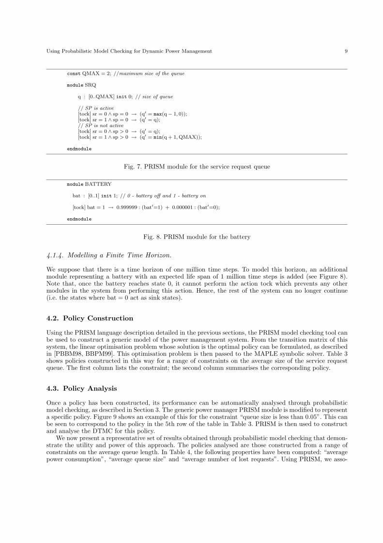
const QMAX = 2; //maximum size of the queue

module SRQ

q : [0..QMAX] init 0; // size of queue

// SP is active[tock] sr = 0 ∧ sp = 0 → (q′ = max(q− 1, 0));[tock] sr = 1 ∧ sp = 0 → (q′ = q);// SP is not active[tock] sr = 0 ∧ sp > 0 → (q′ = q);[tock] sr = 1 ∧ sp > 0 → (q′ = min(q + 1, QMAX));

endmodule

Fig. 7. PRISM module for the service request queue

module BATTERY

bat : [0..1] init 1; // 0 - battery off and 1 - battery on

[tock] bat = 1 → 0.999999 : (bat′=1) + 0.000001 : (bat′=0);

endmodule

Fig. 8. PRISM module for the battery

4.1.4. Modelling a Finite Time Horizon.

We suppose that there is a time horizon of one million time steps. To model this horizon, an additionalmodule representing a battery with an expected life span of 1 million time steps is added (see Figure 8).Note that, once the battery reaches state 0, it cannot perform the action tock which prevents any othermodules in the system from performing this action. Hence, the rest of the system can no longer continue(i.e. the states where bat = 0 act as sink states).

4.2. Policy Construction

Using the PRISM language description detailed in the previous sections, the PRISM model checking tool canbe used to construct a generic model of the power management system. From the transition matrix of thissystem, the linear optimisation problem whose solution is the optimal policy can be formulated, as describedin [PBBM98, BBPM99]. This optimisation problem is then passed to the MAPLE symbolic solver. Table 3shows policies constructed in this way for a range of constraints on the average size of the service requestqueue. The first column lists the constraint; the second column summarises the corresponding policy.

4.3. Policy Analysis

Once a policy has been constructed, its performance can be automatically analysed through probabilisticmodel checking, as described in Section 3. The generic power manager PRISM module is modified to representa specific policy. Figure 9 shows an example of this for the constraint “queue size is less than 0.05”. This canbe seen to correspond to the policy in the 5th row of the table in Table 3. PRISM is then used to constructand analyse the DTMC for this policy.

We now present a representative set of results obtained through probabilistic model checking that demon-strate the utility and power of this approach. The policies analysed are those constructed from a range ofconstraints on the average queue length. In Table 4, the following properties have been computed: “averagepower consumption”, “average queue size” and “average number of lost requests”. Using PRISM, we asso-


Table 3. Optimum policies under varying constraints on the average queue size

constraint optimum policy

6 1.5 if the SP is active and the SRQ is not full thenwith probability 1 goto idle

elseif the SR is idle, the SP is in sleep and the SRQ is full thenwith probability 0.00000047 goto active

elseif the SR is in req and the SP is idle thenwith probability 1 goto active

end

6 1 if the SP is active and the SRQ is not full thenwith probability 1 goto idle



end




end


elseif the SR is idle and the SP is idle thenwith probability 0.95197200 goto active


elseif the SP is in sleep thenwith probability 1 goto active

end

6 0.05 if the SP is active, the SR is idle and the SRQ is empty thenwith probability 0.36316067 goto idle

elseif the SP is idle thenwith probability 1 goto active


end

6 0.001 if the SP is active, the SR is idle and the SRQ is empty thenwith probability 0.05068717 goto idle

elseif the SP is idle thenwith probability 1 goto active


end

ciate a cost with each state and then compute the expected accumulated cost of the system until it reachesa state where the battery has run out. For example, to determine the average power consumption, the costassociated with each state is determined by the state of the SP and the data given in Table 1.

From the table, we can see that the average power consumption of a policy decreases as the constrainton queue size is relaxed (i.e. the requested average queue size is increased). We can also validate the policyby confirming that the expected size of the queue matches the value in the constraint which was used toconstruct it. Finally, we see that a side-effect of this is that the average number of requests lost also increases.

In Figure 10, we show graphical results for a range of policies. Using the same assignments of modelstates to costs as discussed above, we (automatically in PRISM) compute and plot, for a range of values ofT : “expected power consumption by time T”, “expected queue size at time T”, and “expected number of lostrequests by time T”. The first and third properties are determined by computing expected cost cumulated


module PM

// policy when constraint on queue size equals 0.05pm : [0..4]; // 0− go to active, 1− go to idle, 2− go to idlelp, 3− go to standby, 4− go to sleep

[tick] sr=0 ∧ sp=0 ∧ q=0 → 0.63683933 : (pm′=0) // go to active+ 0.36316067 : (pm′=1); // go to idle

[tick] sp=1 ∨ sp=9 → (pm′=0); // go to active[tick] ¬(sp=9 ∨ sp=1 ∨ (sr=0 ∧ sp=0 ∧ q=0)) → (pm′=pm);

endmodule

Fig. 9. PRISM module for the power manager under performance constraint 0.05

Table 4. DTMC case study: Power versus performance

policy average power average queue average numberconstraint consumption size of lost requests

0.001 2.460629 0.001000 0.0001060.05 2.282590 0.050000 0.0001060.1 2.060040 0.100000 0.0001060.2 1.670410 0.200000 0.0016710.3 1.583163 0.300000 0.0117700.4 1.495917 0.400000 0.0218690.5 1.408671 0.500000 0.0319680.6 1.321424 0.600000 0.0420670.7 1.234178 0.700000 0.0521660.8 1.146932 0.800000 0.0622650.9 1.059686 0.900000 0.0723641.0 0.972439 1.000000 0.0824631.1 0.885193 1.100000 0.0925621.2 0.797947 1.200000 0.1026611.3 0.710700 1.300000 0.1127601.4 0.623454 1.400000 0.1228591.5 0.536208 1.500000 0.1329581.6 0.448962 1.600000 0.1430571.7 0.361715 1.700000 0.1531561.8 0.274469 1.800000 0.1632551.9 0.187223 1.900000 0.1733542.0 0.100000 2.000000 0.183450

up until time T ; the second by computing the instantaneous cost at time T . Again, we see that policies whichconsume less power have larger queue sizes and are more likely to lose requests. Here, though, we can get amuch clearer view of how these properties change over time. We see, for example, that the expected queuesize at time T initially increases and then decreases. This follows from the fact that the strategies wait forthe queue to become full before switching the SP on.

Further properties that we can analyse using probabilistic model checking include:

1. the probability that the queue becomes full before time T (P=?[♦62T q=QMAX]);2. the probability that a request is served by time T , given that it arrived into a certain position in the

queue (P=?[♦62T served ]);

3. the probability that N requests get lost by time T (P=?[♦62T lost=N ]).

Note that, in the formulae, we use time-bounds of 2T , as opposed to T , since two steps in the model (a ‘tick’followed by a ‘tock’) correspond to one time-unit in the system. To verify the second and third properties,we must add variables to the PRISM model which record the current position of the request under analysisand to count the number of lost requests (up to a maximum on N), respectively. In Figure 11 we presentthese results for a range of policies and for a range of values of T . The graphs show that:


0 5 100

500

1000

1500

2000

2500

time bound T (102 ms)

expe

cted

pow

er c

onsu

mpt

ion

by T

constraint 0.01constraint 0.05constraint 0.1constraint 0.5constraint 1

0 2 4 6 8 100

0.5

1

1.5

2


expe

cted

que

ue s

ize

at ti

me

T

constraint 1constraint 0.5constraint 0.1constraint 0.05constraint 0.01

0 2 4 6 8 100

50

100

150

200


expe

cted

lost

requ

ests

by

T constraint 1constraint 0.5constraint 0.1constraint 0.05constraint 0.01

Fig. 10. DTMC case study: power and performance by time T (ms) for optimal policies under differentconstraints

0 10 20 30 40 500

0.2

0.4

0.6

0.8

1

time bound T (ms)

prob

abili

ty q

ueue

full

by T

constraint=1constraint=0.5constraint=0.1constraint=0.05constraint=0.01

0 5000 100000

0.2

0.4

0.6

0.8

1

time bound T (ms)

prob

abili

ty re

ques

t ser

ved

by T

constraint=0.05constraint=0.1constraint=0.25constraint=0.5constraint=1

4000 5000 6000 70000

0.2

0.4

0.6

0.8

1

time bound T (ms)

prob

abili

ty 1

000

requ

ests

lost

by

T

constraint=1constraint=0.5constraint=0.25constraint=0.1constraint=0.05

Fig. 11. DTMC case study: analysis of optimal policies for different performance constraints

1. the probability of the queue becoming full within a time bound increases as the constraint on the per-formance is relaxed (i.e. the requested average queue size is increased);

2. the probability that requests get served increases for policies with stricter performance constraints;3. the probability of requests being lost within a certain time bound increases more quickly for the strategies

with weaker performance constraints.

These results confirm that the policies behave as you would expect. In order to reduce power, the strategieswith less strict performance constraints (i.e. with higher values for average queue constraint) can allow theservice provider to spend more time in low power states in which service requests cannot be dealt with, e.g.in sleep and standby. For further details on the results obtained, see the PRISM web page [Pri].

4.4. The Continuous-Time Case

We have also applied probabilistic model checking to the stochastic optimum control approach of [QP99,QWP00, QWP01], which is based on CTMCs rather than DTMCs. The key differences between these twochoices of model were given in Section 2. From the point of view of modelling in PRISM, the two arerelatively similar. The model has the same basic structure: each component (PM, SP, SRQ and SR) is aseparate module and the system is constructed as the parallel composition of these modules. However, inthis case we no longer require the CLOCK module to control synchronisation. Since the model is a CTMC,components change state according to exponentially distributed delays and the PM acts when such a statetransition occurs.

The construction of optimum policies from the PRISM model now follows the approach of [QP99, QWP00,QWP01]. We again use MAPLE to perform the solution of optimisation problems for this purpose. For theanalysis of policies, we can consider similar properties to the DTMC case. As in the DTMC case, there isa power consumption associated with each power state of the SP (per unit of time); however, there is alsoa power usage associated with a change in the SP’s state. The main differences are that we use the logicCSL as opposed to the logic PCTL, and that the time bound T used in the properties is now a real value as


opposed to a number of discrete steps. For details on the results obtained using CSL on this case study seethe PRISM web page [Pri].

Furthermore, in this case, we can also analyse the policies for alternative, more general, inter-arrivaltime distributions, to give a more realistic model of the arrival of service requests (e.g. Pareto). This can beachieved by modelling the DPM system, for a fixed policy, as a time-homogeneous Markov renewal process[Cin75, Kul95] where the renewal point corresponds to the arrival of a new request from the SR. Moreprecisely, we can represent the system as a stochastic process (X, T ) = {Xn, Tn |n ∈ N}, where Xn ∈ S is arandom variable corresponding to the state of the system (i.e the state of SP, SR, SRQ and PM) just beforethe arrival of the nth request and Tn ∈ R>0 is a random variable corresponding to the time of the arrival ofthe nth request.

For the process (X, T ) to be a time-homogeneous Markov renewal process, it must satisfy the followingtwo conditions:

Markovian: for any n ∈ N, s1, . . . , sn+1 ∈ S and t, t1, . . . , tn ∈ R>0:

P(Xn+1=sn+1, Tn+1−Tn 6 t |X0=s0, . . . , Xn=sn;T1=t1, . . . , Tn=tn)= P(Xn+1=sn+1, Tn+1−Tn 6 t |Xn=sn) , (1)

i.e. the probability of state change is history-independent.Time homogeneity: there exists Q : S×S×R>0 → [0, 1] such that for any n ∈ N, s, s′ ∈ S and t ∈ R>0:

P(Xn+1=s′, Tn+1−Tn 6 t |Xn=s) = Q(s, s′, t) , (2)

i.e. the probability of state change is time-independent.

The satisfaction of (1) and (2) for the process (X, T ) considered here follows from the fact that the inter-arrival time distribution is the only non-exponential distribution in the system (and therefore the onlydistribution which is non-Markovian) and that the time between the arrival of nth and (n+1)th request isgiven by the inter-arrival time distribution (and is therefore independent of the time between the arrivals ofprevious requests).

For a time-homogeneous Markov renewal process (X, T ), the family {Q(s, s′, t) | s, s′ ∈ S, t ∈ R>0} iscalled a semi-Markov kernel over S and can be used to construct the embedded DTMC (S,P) of the process,where for any s, s′ ∈ S:

P(s, s′) = limt→∞

Q(s, s′, t) . (3)

More precisely, in the embedded DTMC, the probability of making a transition from state s to s′ is givenby the probability, in the actual process, of being in state s′ just before the arrival of a request given thatthe state of the system was s immediately before the arrival of the previous request.

Now, by considering our model as a time-homogeneous Markov renewal process, we can use the theory ofMarkov renewal processes [Cin75, Kul95] to compute performance metrics of the system. For example, undercertain restrictions, including that the process is aperiodic and irreducible (which hold for the processes weconsider), letting:

C(s, s′) = E(time spent in state s′ during (0, T1) |X0=s) (4)

i.e. the expected time the process spends in state s′ between two renewal points, given that it started instate s after the last renewal, and letting u be the steady state vector of the embedded DTMC, then thelimiting state probabilities vector π of the Markov renewal process are given by:

π =u ·C

u ·C · 1. (5)

The following procedure describes how we have combined probabilistic model checking (in particular themethods given in [KNP02a, KNP02b]) and the theory of Markov renewal processes to analyse the powermanagement policies under general inter-arrival time distributions.

1. Construct a restricted model of the system in which transitions corresponding to new requests are re-moved. Note that, in this restricted model, all transitions have exponential delay, that is, it is a CTMC.

2. Construct the embedded DTMC of the Markov renewal process described above, that is compute the


Table 5. CTMC case study: Power versus performance

performance constraint inter-arrival time distributionmeasure deterministic exponential Erlang uniform Pareto

average 0.1 0.95607 0.95732 0.95624 0.95675 0.96085power 1 0.88649 0.89635 0.88776 0.89168 0.93099

consumption 5 0.64712 0.63498 0.64577 0.64265 0.43536

average 0.1 0.12454 0.10000 0.12124 0.11101 0.028132queue 1 1.2140 1.0000 1.1866 1.0999 0.20238size 5 5.1573 5.0000 5.1399 5.1021 1.6534

average 0.1 2.3677e-06 1.1865e-05 2.9357e-06 4.8316e-06 3.5617e-03number of 1 2.5110e-05 1.3217e-04 3.1335e-05 5.2690e-05 4.4060e-02

lost requests 5 1.9618e-04 1.0033e-03 2.4324e-04 4.1157e-04 3.3341e-01

probabilities given in (3). These are determined by calculating the probability of satisfying random time-bounded until formulae [KNP02a] on the restricted CTMC model where the random time bound T is setequal to the inter-arrival time distribution of requests. More precisely, for any pair s, s′ of states, P(s, s′)is given by the probability, in the restricted CTMC model, of being in state s′ at the random time T ,having started in state s, where the only difference2 between s and s is that in s there is one more requestin the queue (SRQ). In the case where the queue is full, s and s are the same. Note that an alternativeapproach to the construction of the embedded DTMC is to following the methodology of [Ger00].

3. In the restricted CTMC model, calculate, using the techniques developed in [KNP02b], the expectedreward cumulated until the random time T for the following rewards: time spent in a state, powerconsumption, queue size and number of lost requests. For example, when the reward is equal to the timespent in state s′, the expected cumulated reward, starting from state s, gives the the values C(s, s′) of (4),where the difference between s and s is as in step 2. When the reward is equal to the power consumption,the expected cumulated reward gives the expected power consumption between renewal points.

4. Using the theory of Markov renewal processes, calculate performance and power metrics of the system,through the analysis of the embedded DTMC constructed in step 2 and the expected reward valuescomputed in step 3. For example, the long-run average power consumption can be computed by combiningthe limiting state probabilities and the expected power consumption between two renewal points of therenewal process. The limiting state probabilities are computed using (5) (i.e. combining the steady stateprobabilities of the DTMC constructed in step 2 and the values C(s, s′) computed in step 3) and theexpected expected power consumption between two renewal points is calculated in step 3.

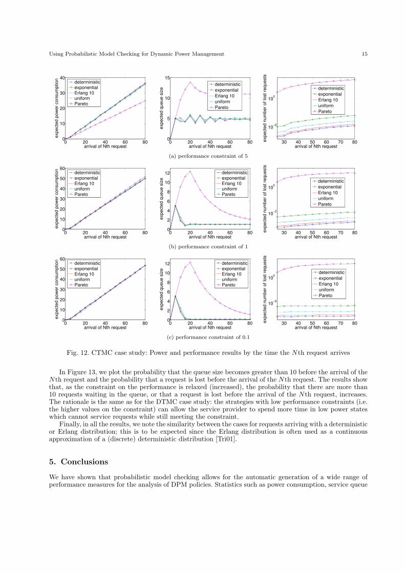
We now present a selection of results to illustrate the utility of the procedure described above. Table 5shows average power consumption, average queue size and average number of lost requests for optimumpolicies under five different inter-arrival distributions. The distributions chosen all have the same mean andit can be seen that, with the exception of the Pareto distribution, the long-run performance and costs arereasonably close to those of the exponential arrival process. For the Pareto distribution, the average queuesize is generally much smaller. This is a result of the Pareto distribution’s heavy tail , which means that,in the long run, many requests will not arrive for a very long time, and hence, in these cases, the serviceprovider (SP) will serve all pending requests, and then the system will spend a long time with the queueempty and the SP in its sleep state consuming very little power. Moreover, more requests are blocked forthe Pareto distribution than with the other distributions.

In Figure 12, we present the power and performance results up until the arrival of the Nth request as theinter-arrival time distribution varies for the optimum policies for the cases when the constraint on the queuesize is 5, 1 and 0.1. Note that, since the distributions we consider have the same mean, the expected arrivaltime of the Nth request is the same for all the distributions considered. Again, we see that the results arevery similar in all cases except when the inter-arrival time has a Pareto distribution. Comparing the resultswe see that, as for the DTMC case study, for larger constraints the power consumption decreases while theexpected queue size and expected number of lost requests increases.

2 Recall that Xn corresponds to the state of the system immediately before the arrival of the nth request.


0 20 40 60 800

10

20

30

40

arrival of Nth request

expe

cted

pow

er c

onsu

mpt

ion deterministic

exponentialErlang 10uniformPareto

0 20 40 60 800

5

10

15


expe

cted

que

ue s

ize

deterministicexponentialErlang 10uniformPareto

30 40 50 60 70 80

10−2

100


expe

cted

num

ber o

f los

t req

uest

s


(a) performance constraint of 5

0 20 40 60 800

10

20

30

40

50

60


expe

cted

pow

er c

onsu

mpt

ion deterministic


0 20 40 60 800

2

4

6

8

10

12


expe

cted

que

ue s

ize


30 40 50 60 70 80

10−2

100


expe

cted

num

ber o

f los

t req

uest

s


(b) performance constraint of 1

0 20 40 60 800

10

20

30

40

50

60


expe

cted

pow

er c

onsu

mpt

ion deterministic


0 20 40 60 800

2

4

6

8

10

12


expe

cted

que

ue s

ize


30 40 50 60 70 80

10−2

100


expe

cted

num

ber o

f los

t req

uest

s


(c) performance constraint of 0.1

Fig. 12. CTMC case study: Power and performance results by the time the Nth request arrives

In Figure 13, we plot the probability that the queue size becomes greater than 10 before the arrival of theNth request and the probability that a request is lost before the arrival of the Nth request. The results showthat, as the constraint on the performance is relaxed (increased), the probability that there are more than10 requests waiting in the queue, or that a request is lost before the arrival of the Nth request, increases.The rationale is the same as for the DTMC case study: the strategies with low performance constraints (i.e.the higher values on the constraint) can allow the service provider to spend more time in low power stateswhich cannot service requests while still meeting the constraint.

Finally, in all the results, we note the similarity between the cases for requests arriving with a deterministicor Erlang distribution; this is to be expected since the Erlang distribution is often used as a continuousapproximation of a (discrete) deterministic distribution [Tri01].

5. Conclusions

We have shown that probabilistic model checking allows for the automatic generation of a wide range ofperformance measures for the analysis of DPM policies. Statistics such as power consumption, service queue


0 20 40 60 800

0.2

0.4

0.6

0.8

1

prob

abili

ty q

ueue

≥ 1

0


deterministicexponentialErlang 10uniform[0,b]Pareto

(a) performance constraint of 5

0 20 40 60 800

0.2

0.4

0.6

0.8

1

prob

abili

ty q

ueue

≥ 1

0



(b) performance constraint of 1

0 20 40 60 800

0.2

0.4

0.6

0.8

prob

abili

ty q

ueue

≥ 1

0



(c) performance constraint of 0.1

0 500 1000 1500 20000

0.2

0.4

0.6

0.8

1

prob

abili

ty c

usto

mer

is lo

st

Nth request arrives


(d) performance constraint of 5

0 500 1000 1500 20000

0.2

0.4

0.6

0.8

1

prob

abili

ty c

usto

mer

is lo

st

Nth request arrives


(e) performance constraint of 1

0 500 1000 1500 20000

0.1

0.2

0.3

0.4

0.5

0.6

prob

abili

ty c

usto

mer

is lo

st

Nth request arrives


(f) performance constraint of 0.1

Fig. 13. CTMC case study: analysis of optimal policies for different performance constraints

length and the number of requests lost can be computed, both in the average case and for particular timeinstances over a given range. The fact that a constructed policy is only known to be optimal in the averagecase makes this information particularly interesting. Furthermore, the policies’ behaviour can be examinedunder alternative, more realistic, service request inter-arrival time distributions such as Erlang and Pareto.

An inherent advantage of the model checking approach is that the analysis of the state-space is exhaustive,in contrast to, say, simulation. This means that the answers computed are guaranteed to be accurate withrespect to the probabilistic model used, and that all behaviour, including corner-case scenarios, is considered.We are presently extending this work by building an analytical framework that derives and analyses strategiesfor more general probabilistic assumptions. We are also considering applying our methodology to DPMschemes with multiple power-managed devices.

Acknowledgements

This work was supported by NSF grants CCR-0098335 and CCR-0340740, EPSRC grants GR/N22960 andGR/S11107, FORWARD, SRC, and DARPA/ITO supported PADS project under the PAC/C program.

References

[ACP] Advanced configuration and power interface website (www.acpi.info).[AH99] R. Alur and T. Henzinger. Reactive modules. Formal Methods in System Design, 15:7–48, 1999.[ASSB96] A. Aziz, K. Sanwal, V. Singhal, and R. Brayton. Verifying continuous time Markov chains. In R. Alur and

T. Henzinger, editors, Proc. 8th Int. Conf. Computer Aided Verification (CAV’96), volume 1102 of Lecture Notesin Computer Science, pages 269–276. Springer-Verlag, 1996.

[BBM00] L. Benini, A Bogliolo, and G. De Micheli. A survey of design techniques for system-leveldynamic power management.IEEE Transactions on Very Large Scale Integration (TVLSI) Systems, 8(3):299–316, 2000.

[BBPM99] L. Benini, A Bogliolo, G. Paleologo, and G. De Micheli. Policy optimization for dynamic power management. IEEETransactions on Computer-Aided Design of Integrated Circuits and Systems, 18(6):813–833, 1999.

[BdA95] A. Bianco and L. de Alfaro. Model checking of probabilistic and nondeterministic systems. In P. Thiagarajan,


editor, Proc. 15th Conf. Foundations of Software Technology and Theoretical Computer Science, volume 1026 ofLecture Notes in Computer Science, pages 499–513. Springer-Verlag, 1995.

[Ber95] D. Bertsekas. Dynamic Programming and Optimal Control, Volumes 1 and 2. Athena Scientific, 1995.[BHHK00] C. Baier, B. Haverkort, H. Hermanns, and J.-P. Katoen. On the logical characterisation of performability proper-

ties. In U. Montanari, J. Rolim, and E. Welzl, editors, Proc. 27th Int. Colloquium on Automata, Languages andProgramming (ICALP’00), volume 1853 of Lecture Notes in Computer Science, pages 780–792. Springer-Verlag,2000.

[BKH99] C. Baier, J.-P. Katoen, and H. Hermanns. Approximate symbolic model checking of continuous-time Markovchains. In J. Baeten and S. Mauw, editors, Proc. 10th Int. Conf. Concurrency Theory (CONCUR’99), volume1664 of Lecture Notes in Computer Science, pages 146–161. Springer-Verlag, 1999.

[BM98] L. Benini and G. De Micheli. Dynamic Power Management: Design Techniques and CAD Tools. Kluwer Publica-tions, 1998.

[BMM01] L. Benini, G. De Micheli, and E. Macii. Designing low-power circuits: Practical recipes. IEEE Circuits and SystemsMagazine, 1(1):6–25, 2001.

[BT91] D. Bertsekas and J. Tsitsiklis. An analysis of stochastic shortest path problems. Mathematics of OperationsResearch, 16(3):580–595, 1991.

[CBBM99] E.-Y. Chung, L. Benini, A. Bogliolo, and G. De Micheli. Dynamic power management for non-stationary servicerequests. In Proc. Design, Automation and Test in Europe (DATE’99), pages 77–81. IEEE Computer SocietyPress, 1999.

[Cin75] E. Cinlar. Introduction to Stochastic Processes. Prentice Hall, 1975.[dA97] L. de Alfaro. Formal Verification of Probabilistic Systems. PhD thesis, Stanford University, 1997.[Ger00] R. German. Performance Analysis of Communication Systems: Modeling with Non-Markovian Stochastic Petri

Nets. John Wiley and Sons, 2000.[HAW96] C.-H. Hwang, C. Allen, and H. Wu. A predictive system shutdown method for energy saving of event-driven

computation. In Proc. Int. Conf. on Computer-Aided Design (ICCAD’97), pages 28–32. IEEE Computer SocietyPress, 1996.

[HGCC99] V. Hartonas-Garmhausen, S. Campos, and E. Clarke. ProbVerus: Probabilistic symbolic model checking. In J.-P.Katoen, editor, Proc. 5th Int. AMAST Workshop on Real-Time and Probabilistic Systems (ARTS’99), volume1601 of Lecture Notes in Computer Science, pages 96–110. Springer-Verlag, 1999.

[HJ94] H. Hansson and B. Jonsson. A logic for reasoning about time and probability. Formal Aspects of Computing,6:512–535, 1994.

[HKMKS00] H. Hermanns, J.-P. Katoen, J. Meyer-Kayser, and M. Siegle. A Markov chain model checker. In S. Graf andM. Schwartzbach, editors, Proc. 6th Int. Conf. Tools and Algorithms for the Construction and Analysis of Systems(TACAS 2000), volume 1785 of Lecture Notes in Computer Science, pages 347–362. Springer-Verlag, 2000.

[IBM] Technical specifications of hard drive IBM Travelstar VP (www.storage.ibm.com/storage/oem/data/travvp.htm).[ISG02] S. Irani, S. Shukla, and R. Gupta. Competitive analysis of dynamic power management strategies for systems with

multiple power saving states. In Proc. Design Automation and Test Conference (DATE 2002), pages 117–123.IEEE Computer Society Press, 2002.

[JDL02] B. Jeannet, P. D’Argenio, and K. Larsen. Rapture: A tool for verifying Markov decision processes. In I. Cerna,editor, Proc. Tools Day, affiliated to 13th Int. Conf. Concurrency Theory (CONCUR’02), Technical Report FIMU-RS-2002-05, Faculty of Informatics, Masaryk University, pages 84–98, 2002.

[KNP02a] M. Kwiatkowska, G. Norman, and A. Pacheco. Model checking CSL until formulae with random time bounds. InH. Hermanns and R. Segala, editors, Proc. 2nd Joint Int. Workshop on Process Algebra and Probabilistic Meth-ods, Performance Modeling and Verification (PAPM/PROBMIV’02), volume 2399 of Lecture Notes in ComputerScience, pages 152–168. Springer-Verlag, 2002.

[KNP02b] M. Kwiatkowska, G. Norman, and A. Pacheco. Model checking expected time and expected reward formulae withrandom time bounds. In Proc. 2nd Euro-Japanese Workshop on Stochastic Risk Modelling for Finance, Insurance,Production and Reliability, 2002.

[KNP04] M. Kwiatkowska, G. Norman, and D. Parker. PRISM 2.0: A tool for probabilistic model checking. In Proc.1st International Conference on Quantitative Evaluation of Systems (QEST’04), pages 322–323. IEEE ComputerSociety Press, 2004.

[Kul95] V. Kulkarni. Modeling and Analysis of Stochastic Systems. Chapman and Hall, 1995.[Map] MapleSoft Corporation. Maple computer algebra system (www.maplesoft.com).[Mic98] Microsoft corporation, OnNow power management architecture for applications (msdn.microsoft.com/library/en-

us/dndevio/html/onnowapp.asp). 1998.[NPK+02] G. Norman, D. Parker, M. Kwiatkowska, S. Shukla, and R. Gupta. Formal analysis and validation of continuous

time Markov chain based system level power management strategies. In W. Rosenstiel, editor, Proc. 7th AnnualIEEE Int. Workshop on High Level Design Validation and Test (HLDVT’02), pages 45–50. IEEE ComputerSociety Press, 2002.

[NPK+03] G. Norman, D. Parker, M. Kwiatkowska, S. Shukla, and R. Gupta. Using probabilistic model checking for dynamicpower management. In M. Leuschel, S. Gruner, and S. Lo Presti, editors, Proc. 3rd Workshop on AutomatedVerification of Critical Systems (AVoCS’03), Technical Report DSSE-TR-2003-2, University of Southampton,pages 202–215, 2003.

[Par02] D. Parker. Implementation of Symbolic Model Checking for Probabilistic Systems. PhD thesis, University ofBirmingham, 2002.

[PBBM98] G. Paleologo, L. Benini, A. Bogliolo, and G. Micheli. Policy optimization for dynamic power management. In Proc.35th Conf. Design Automation (DAC 1998), pages 182–187. ACM Press, 1998.


[Pri] PRISM web page (www.cs.bham.ac.uk/∼dxp/prism).[QP99] Q. Qiu and M. Pedram. Dynamic power management based on continuous-time Markov decision processes. In

Proc. 36th Conf. Design Automation (DAC 1999), pages 555–561, 1999.[QWP00] Q. Qiu, Q. Wu, and M. Pedram. Dynamic power management of complex systems using generalized stochastic

Petri nets. In Proc. 37th Conf. Design Automation (DAC 2000), pages 352–356, 2000.[QWP01] Q. Qiu, Q. Wu, and M. Pedram. Stochastic modeling of a power-managed system: construction and optimization.

IEEE Transactions on Computer Aided Design, 20(9):1200–1217, 2001.[RIG00] D. Ramanathan, S. Irani, and R. Gupta. Latency effects of system level power management algorithms. In Proc.

IEEE Int. Conf. Computer-Aided Design, 2000.[SBM99] T. Simunic, L. Benini, and G. De Micheli. Event driven power management of portable systems. In Proc. Int.

Symp. System Synthesis (ISSS 1999), pages 18–23. IEEE Computer Society Press, 1999.[SCB96] M. Srivastava, A. Chandrakasan, and R. Broderson. Predictive shutdown and other architectural techniques for

energy efficient programmable computation. IEEE Trans. on VLSI Systems, 4(1):42–54, 1996.[SG01] S. Shukla and R. Gupta. A model checking approach to evaluating system level power management for embedded

systems. In Proc. IEEE Workshop on High Level Design Validation and Test (HLDVT’01), pages 53–57. IEEEComputer Society Press, 2001.

[Tri01] K. Trivedi. Probability and Statistics with Reliability, Queuing, and Computer Science Applications. John Wileyand Sons, 2001.

Documents

Using Probabilistic Model Checking for Dynamic …parkerdx/papers/power.fac.pdfUsing Probabilistic Model Checking for ... Power management, formal methods, embedded systems, ... Using