Embed Size (px)
Citation preview

USING PRIMARY AFFERENT NEURAL
ACTIVITY FOR PREDICTING LIMB
KINEMATICS IN CAT
by
J. B. M. Wagenaar
M.S. in Electrical Engineering
University of Twente, 2005
Submitted to the Graduate Faculty of
the Swanson School of Engineering in partial fulfillment
of the requirements for the degree of
Doctor of Philosophy
University of Pittsburgh
2011

UNIVERSITY OF PITTSBURGH
SWANSON SCHOOL OF ENGINEERING
This dissertation was presented
by
J. B. M. Wagenaar
It was defended on
March 25th 2011
and approved by
D.J. Weber, Ph.D., Professor, Bioengineering Department
V. Ventura, Ph.D., Professor, Statistics Department, Carnegie Mellon University
A.B. Schwartz, Ph.D., Professor, Neurobiology Department
B.J. Yates, Ph.D., Professor, Neuroscience Department
C.G. Atkeson, Ph.D., Professor, Robotics Department, Carnegie Mellon University
Dissertation Director: D.J. Weber, Ph.D., Professor, Bioengineering Department
ii

Copyright c© by J. B. M. Wagenaar
2011
iii

USING PRIMARY AFFERENT NEURAL ACTIVITY FOR PREDICTING
LIMB KINEMATICS IN CAT
J. B. M. Wagenaar, PhD
University of Pittsburgh, 2011
Kinematic state feedback is important for neuroprostheses to generate stable and adaptive
movements of an extremity. State information, represented in the firing rates of populations
of primary afferent neurons, can be recorded at the level of the dorsal root ganglia (DRG).
Previous work in cats showed the feasibility of using DRG recordings to predict the kinematic
state of the hind limb using reverse regression. Although accurate decoding results were
attained, these methods did not make efficient use of the information embedded in the firing
rates of the neural population.
This dissertation proposes new methods for decoding limb kinematics from primary af-
ferent firing rates. We present decoding results based on state-space modeling, and show
that it is a more principled and more efficient method for decoding the firing rates in an
ensemble of primary afferent neurons. In particular, we show that we can extract confounded
information from neurons that respond to multiple kinematic parameters, and that includ-
ing velocity components in the firing rate models significantly increases the accuracy of the
decoded trajectory.
This thesis further explores the feasibility of decoding primary afferent firing rates in the
presence of stimulation artifact generated during functional electrical stimulation. We show
that kinematic information extracted from the firing rates of primary afferent neurons can
be used in a real-time application as a feedback for control of FES in a neuroprostheses. It
provides methods for decoding primary afferent neurons and sets a foundation for further
development of closed loop FES control of paralyzed extremities.
iv

Although a complete closed loop neuroprosthesis for natural behavior seems far away, the
premise of this work argues that an interface at the dorsal root ganglia should be considered
as a viable option.
Keywords: bioengineering, muscle spindle, primary afferent, nervous system, closed loop
control, state-space modeling, neuroprostheses, FES .
v

TABLE OF CONTENTS
1.0 INTRODUCTION . . . . . . . . . . . . . . . . . . . . . . . . . . . . . . . . . 1
1.1 SENSORIMOTOR PHYSIOLOGY . . . . . . . . . . . . . . . . . . . . . . . 1
1.1.1 Advances towards understanding the sensory nervous system. . . . . . 1
1.1.2 Firing rate properties of primary afferent neurons . . . . . . . . . . . 3
1.1.2.1 The muscle spindle . . . . . . . . . . . . . . . . . . . . . . . . 3
1.1.2.2 Other afferent neurons . . . . . . . . . . . . . . . . . . . . . . 7
1.1.3 Proprioceptive coordinate frame . . . . . . . . . . . . . . . . . . . . . 8
1.1.4 Role of somatosensory afferents in regulating motor output . . . . . . 12
1.1.5 The impact of spinal cord injury to primary afferent response . . . . . 13
1.2 USING AFFERENT INFORMATION FOR NEURAL PROSTHESES . . . 14
1.2.1 Using primary afferent or external sensors? . . . . . . . . . . . . . . . 14
1.2.2 Sensorimotor control as a closed loop control system . . . . . . . . . . 15
1.2.3 Neural interfaces . . . . . . . . . . . . . . . . . . . . . . . . . . . . . . 17
1.2.4 Inferring limb state from afferent activity . . . . . . . . . . . . . . . . 18
1.2.5 Closed-loop control of FES using natural sensors . . . . . . . . . . . . 20
1.3 SPECIFIC AIMS . . . . . . . . . . . . . . . . . . . . . . . . . . . . . . . . . 21
1.3.1 Direct decoding of primary afferent neuron firing rates . . . . . . . . . 21
1.3.2 State-space decoding of primary afferent neuron firing rates . . . . . . 22
1.3.3 Improved decoding techniques for realtime applications. . . . . . . . . 22
1.3.4 Closed loop FES using primary afferent response as feedback . . . . . 23
2.0 IMPROVED DECODING OF LIMB-STATE FEEDBACK FROM NAT-
URAL SENSORS . . . . . . . . . . . . . . . . . . . . . . . . . . . . . . . . . 24
vi

2.1 INTRODUCTION . . . . . . . . . . . . . . . . . . . . . . . . . . . . . . . . 24
2.2 METHODS AND DATA . . . . . . . . . . . . . . . . . . . . . . . . . . . . . 25
2.2.1 The experiment . . . . . . . . . . . . . . . . . . . . . . . . . . . . . . 25
2.2.2 Reverse regression . . . . . . . . . . . . . . . . . . . . . . . . . . . . . 27
2.2.3 Direct regression methods . . . . . . . . . . . . . . . . . . . . . . . . . 27
2.2.4 Contrasting methods . . . . . . . . . . . . . . . . . . . . . . . . . . . 29
2.3 RESULTS . . . . . . . . . . . . . . . . . . . . . . . . . . . . . . . . . . . . . 29
2.4 DISCUSSION . . . . . . . . . . . . . . . . . . . . . . . . . . . . . . . . . . . 33
3.0 STATE-SPACE DECODING OF PRIMARY AFFERENT FIRING RATES 36
3.1 INTRODUCTION . . . . . . . . . . . . . . . . . . . . . . . . . . . . . . . . 36
3.2 METHODS AND DATA . . . . . . . . . . . . . . . . . . . . . . . . . . . . . 38
3.2.1 Surgical procedures . . . . . . . . . . . . . . . . . . . . . . . . . . . . 38
3.2.2 The experiment . . . . . . . . . . . . . . . . . . . . . . . . . . . . . . 38
3.2.3 Current decoding paradigm: reverse regression . . . . . . . . . . . . . 41
3.2.4 Firing rate models and likelihood decoding . . . . . . . . . . . . . . . 43
3.2.4.1 Firing rate models in joint angle frame . . . . . . . . . . . . . 44
3.2.4.2 Firing rate models in limb end point frame . . . . . . . . . . 45
3.2.5 State-space models . . . . . . . . . . . . . . . . . . . . . . . . . . . . 45
3.2.5.1 Kinematic models . . . . . . . . . . . . . . . . . . . . . . . . 48
3.2.6 Decoding efficiency . . . . . . . . . . . . . . . . . . . . . . . . . . . . 50
3.2.7 State space algorithm for decoding limb state . . . . . . . . . . . . . . 51
3.2.8 Details for solving eq. 3.6 . . . . . . . . . . . . . . . . . . . . . . . . . 54
3.3 RESULTS . . . . . . . . . . . . . . . . . . . . . . . . . . . . . . . . . . . . . 54
3.3.1 Encoding models . . . . . . . . . . . . . . . . . . . . . . . . . . . . . . 55
3.3.2 Decoding joint angles . . . . . . . . . . . . . . . . . . . . . . . . . . . 57
3.3.3 Decoding endpoint coordinates . . . . . . . . . . . . . . . . . . . . . . 62
3.4 DISCUSSION . . . . . . . . . . . . . . . . . . . . . . . . . . . . . . . . . . . 64
3.4.1 State-space decoding methods of primary afferent activity . . . . . . . 64
3.4.2 Natural feedback for FES control . . . . . . . . . . . . . . . . . . . . . 67
3.5 CONCLUSIONS . . . . . . . . . . . . . . . . . . . . . . . . . . . . . . . . . 68
vii

4.0 ALTERNATIVE DECODING TECHNIQUES FOR PREDICTING LIMB
STATE . . . . . . . . . . . . . . . . . . . . . . . . . . . . . . . . . . . . . . . . 70
4.1 DYNAMIC FUZZY NEURAL NETWORKS . . . . . . . . . . . . . . . . . 70
4.1.1 Alternative implementation of the GD-FNN . . . . . . . . . . . . . . . 73
4.2 SPLINE REVERSE REGRESSION . . . . . . . . . . . . . . . . . . . . . . 79
5.0 CLOSED LOOP CONTROL OF FUNCTIONAL ELECTRICAL STIM-
ULATION . . . . . . . . . . . . . . . . . . . . . . . . . . . . . . . . . . . . . . 82
5.1 INTRODUCTION . . . . . . . . . . . . . . . . . . . . . . . . . . . . . . . . 82
5.2 METHODS . . . . . . . . . . . . . . . . . . . . . . . . . . . . . . . . . . . . 84
5.2.1 Surgical procedures . . . . . . . . . . . . . . . . . . . . . . . . . . . . 84
5.2.2 Experiment setup . . . . . . . . . . . . . . . . . . . . . . . . . . . . . 85
5.2.3 Realtime encoding of firing rate models . . . . . . . . . . . . . . . . . 87
5.2.4 Removing stimulation artifact . . . . . . . . . . . . . . . . . . . . . . 88
5.3 RESULTS . . . . . . . . . . . . . . . . . . . . . . . . . . . . . . . . . . . . . 91
5.3.1 Realtime decoding of primary afferents . . . . . . . . . . . . . . . . . 91
5.3.2 Decoding during stimulation . . . . . . . . . . . . . . . . . . . . . . . 94
5.3.3 Closed loop control of FES . . . . . . . . . . . . . . . . . . . . . . . . 96
5.4 DISCUSSION . . . . . . . . . . . . . . . . . . . . . . . . . . . . . . . . . . . 98
6.0 GENERAL DISCUSSION . . . . . . . . . . . . . . . . . . . . . . . . . . . . 102
6.1 SUMMARY . . . . . . . . . . . . . . . . . . . . . . . . . . . . . . . . . . . . 102
6.2 SIGNIFICANCE AND FUTURE WORK . . . . . . . . . . . . . . . . . . . 104
6.3 FINAL THOUGHTS . . . . . . . . . . . . . . . . . . . . . . . . . . . . . . . 108
BIBLIOGRAPHY . . . . . . . . . . . . . . . . . . . . . . . . . . . . . . . . . . . . 109
viii

LIST OF TABLES
1 Summary of firing rate models . . . . . . . . . . . . . . . . . . . . . . . . . . 46
ix

LIST OF FIGURES
1 Example firing rates of primary afferents during passive movement . . . . . . 4
2 Example of muscle spindle response to succinylcholine . . . . . . . . . . . . . 6
3 Regression models in different coordinate frames . . . . . . . . . . . . . . . . 10
4 Comparison of coordinate frames . . . . . . . . . . . . . . . . . . . . . . . . . 11
5 Schematic representation of motor control . . . . . . . . . . . . . . . . . . . . 16
6 Setup of the experiment . . . . . . . . . . . . . . . . . . . . . . . . . . . . . . 26
7 Example of decoded trajectories. . . . . . . . . . . . . . . . . . . . . . . . . . 30
8 Afferent responses to variations in kinematic variables . . . . . . . . . . . . . 32
9 Summary of results. . . . . . . . . . . . . . . . . . . . . . . . . . . . . . . . . 34
10 Experiment setup 1 . . . . . . . . . . . . . . . . . . . . . . . . . . . . . . . . 39
11 Observed kinematics and neural response . . . . . . . . . . . . . . . . . . . . 49
12 Random walk demonstration . . . . . . . . . . . . . . . . . . . . . . . . . . . 50
13 Example firing rate response . . . . . . . . . . . . . . . . . . . . . . . . . . . 56
14 Summary of results . . . . . . . . . . . . . . . . . . . . . . . . . . . . . . . . 58
15 Example decoded trajectory . . . . . . . . . . . . . . . . . . . . . . . . . . . 60
16 Summary of results . . . . . . . . . . . . . . . . . . . . . . . . . . . . . . . . 61
17 Summary of endpoint decoding results . . . . . . . . . . . . . . . . . . . . . 63
18 Modeling non-linear functions using fuzzy logic. . . . . . . . . . . . . . . . . . 71
19 Simple example of fuzzy logic neural network. . . . . . . . . . . . . . . . . . . 77
20 Decoding center-out movement using fuzzy neural network . . . . . . . . . . . 78
21 Decoding center-out movement using spline reverse regression . . . . . . . . . 80
22 Experiment setup for closed loop FES . . . . . . . . . . . . . . . . . . . . . . 86
x

23 Effects of blanking input . . . . . . . . . . . . . . . . . . . . . . . . . . . . . 89
24 Schematic for removing stimulation artifacts. . . . . . . . . . . . . . . . . . . 90
25 Realtime encoding and decoding of the firing rates of primary afferents . . . . 92
26 Progression of regression coefficients during model encoding . . . . . . . . . . 93
27 Primary afferent firing rates during FES 1 . . . . . . . . . . . . . . . . . . . . 95
28 Decoding ground reaction forces during functional electrical stimulation . . . 95
29 Primary afferent firing rates during FES 2 . . . . . . . . . . . . . . . . . . . . 97
30 Closed loop FES traces and stick-figure of hind limb . . . . . . . . . . . . . . 99
xi

1.0 INTRODUCTION
This chapter introduces the research topics discussed in document. Biomedical engineering
and in particular the neural engineering fields heavily rely upon both physiology of the
nervous system and the engineering aspects in science. Both aspects will be discussed in this
chapter followed by a section outlining the specific aims addressed in this work.
1.1 SENSORIMOTOR PHYSIOLOGY
Scientific discoveries unraveling the purpose and properties of primary afferent firing rates
will be discussed, followed by a section describing the current technology available for using
primary afferent neurons as an integrated part of a neural prosthesis.
1.1.1 Advances towards understanding the sensory nervous system.
Around the year 100 AD, Marinus described the 10th cranial nerve based on anatomic
findings in human. It took approximately 1900 years (1889) before Cajal initiated a series
of discoveries that lead to our current understanding of the nervous system as a complex
network of individual neurons. Only 120 years after Cajal, the first interface with the vagus
nerve was approved by the FDA as a treatment for people with Epilepsy. This shows a clear
picture of the incredible advances have been made in neuroscience during the last century
and might show a glimmer of the possibilities in the future.
Between 1889 and now, incremental scientific discoveries exposed the importance and
complexity of the sensory nervous system. Quickly after Cajal’s discovery, Camillo Golgi
1

described the Golgi tendon organ in 1896, followed by the discovery of the ruffini endings
by Ruffini in 1898. Although the muscle spindle structure was described by Hassal in 1851,
Kerschner was the first to suggest that it was a sensory receptor in 1888. This was later
confirmed in 1894 when Sherrington described how muscle spindles remain intact in muscles
from which all motor fibers have been removed by degeneration after cutting the ventral
roots. He could therefore conclude that muscle spindles are innervated by fibers connecting
to the dorsal roots of the spinal cord and are therefore related the sensory nervous system
[101].
Electric fields resulting from muscle activity and stretch had been described since the
second half of the eighteen-hundreds. However, nobody had recorded the response from
single afferent fibers until 1926 [57]. That year, Adrian and Zotterman recorded from frog’s
sciatic nerve and showed that by sectioning part of the muscle, they could isolate a single
afferent neuron [1]. They concluded that: 1) the afferent firing rate was a function of the
muscle load, 2) There is an all or nothing response by the neuron and 3) There is adaption
of the neuron’s excitability which they attributed to a change in the refractory period [2].
Adrian and Sherrington would receive the Nobel Prize for their work on the function of
neurons in 1932.
The term proprioception was first coined by Sherrington in 1906 to indicate the awareness
of movement from afferent information [102]. It originates from the integration of afferent
inputs in the central nervous system (CNS), provides vital information about the state of
the limb during movement and serves as feedback during motor control to create stable and
accurate movements. Although the exact pathways leading to movement perception are not
fully understood, science is continuously trying to understand the underlying sensory system.
During the 1950’s, the mechanisms responsible for the discrete responses from the sen-
sory neurons were unraveled when intracellular recordings enabled Hodgkin and Huxley to
perform their famous work on the giant axon of squid [49, 48]. Their discoveries have since
been the foundation of a plurality of modeling the nervous system at a cellular level [74].
Research by Adrian and others laid the foundation for more detailed analysis of the
function of the sensory nervous system in later years. Leading into the second half of the
century, technological improvements lead to increasingly accurate data on afferent behavior,
2

the ability to record from multiple neurons simultaneously and the realization that targeted
stimulation of neurons could evoke sensory perceptions [104]. Continuing today, research is
being conducted to understand the role of the sensory nervous system in our everyday life
and how we can utilize the information that the sensory nervous system provides in devices
aimed at restoring extremity functionality in physically impaired people.
1.1.2 Firing rate properties of primary afferent neurons
This section will discuss some of the firing rate properties of primary afferent neurons. Insight
in the firing rate response of primary afferent to kinematic perturbations will be used in later
chapters as a basis for algorithms to estimate limb kinematics.
1.1.2.1 The muscle spindle In contrary to earlier beliefs that the muscle spindles are
the only sensory receptor involved in proprioception, the current thought includes other
afferent types as contributors to proprioception. However, the muscle spindle is still thought
to be the main contributor [35]. An example of muscle spindle response to passive kinematic
movement is shown in figure 1. Here, the limb was manipulated through a series of ramp and
hold patterns in different directions. The cartesian coordinates of the metatarsophalangeal
joint and the instantaneous firing rate of six muscle spindle afferents are plotted over time.
Various models with increasing complexity have been proposed for the muscle spindle
firing rate [68, 51, 80, 82, 66, 72]. These models are able to provide accurate predictions
of spindle firing rates as a function of muscle length and presumed gamma drive inputs.
A thorough classification of the muscle spindle and the afferents innervating the sensory
receptor was described as early as 1963 by Matthews. He identified two groups of afferents
originating from the muscle spindle; group 1 afferents (primary endings) and group 2 afferents
(secondary endings). In addition, he described two efferent fibers innervating the spindle; γ1
motor neurons and γ2 motor neurons [68].
3

Figure 1: Example firing rates of primary afferents during passive movement. A) Cartesian
coordinates of the metatarsophalangeal joint B) Muscle length estimates using the Goslow
model [40] C) Instantaneous firing rates of 6 primary afferent neurons
4

In 1969, Matthews and Stein discussed the muscle spindle firing rate in terms of its
response to sinusoidal muscle stretch and concluded that muscle spindle response is definitely
non-linear in contrast to beliefs at the time [69]. In addition, there experiments showed that
muscle spindle output could significantly be increased when they stimulated the γ- motor
neuron innervating the spindle [69].
More recent work investigating the properties of the muscle spindle suggests that the
classification between two types of γ- motor neurons might be too simple and more work
is needed to understand the system [113, 72]. Mileusnic et al. presented the most complex
muscle spindle model in 2007. Their model consists of 22 model parameters and is a clear
demonstration that muscle spindle modeling is still a daunting task [72].
Alneas et al. found that background fusimotor activity in spinalized cat marked an
increase in the dynamic frequency of the firing rate of the primary muscle spindle neurons
but only slightly increased their response to static extensions [3]. The neural basis for gamma
motor drive has been topic for discussion for many years and various hypotheses have been
put forward. Prochazka et al. compared muscle spindle response in freely moving cats with
those recorded under anesthesia and found that gamma drive is likely set by the CNS to
different levels depending on the performed task [83]. A similar conclusion was reached by
Taylor at al. in 2000 when looking at decerebrate preparations [113].
A muscle spindle neuron can easily be detected from a neural pool of afferent responses
by its combined dynamic and static components of the firing rate response during a ramp and
hold flexion and extension of the muscle. In addition, an intravenous injection of succinyl-
choline will temporarily paralyze the muscles while increasing the muscle spindle response
[87, 114]. Figure 2 shows an example of a muscle spindle response during flexion/extension
of the muscle during a succinylcholine injection. At the beginning of the trial, the succinyl-
choline is administered intravenously and the instantaneous firing rate of the muscle spindle
is plotted for the following 10 minutes. It can be seen clearly that the instantaneous firing
rate of the neuron increases after administration of the drug and that the effect diminishes
over time. In addition, we can see the difference between the dynamic and static contri-
butions of the instantaneous firing rate increases (dynamic index) which is a well described
phenomenon [87].
5

0 100 200 300 400 500 600 7000
62 64 660
100 102 1040
442 444 4460
12 14 16 180
10
20
30
40
50
60
70
80
90
10
20
30
40
50
60
70
80
90
10
20
30
40
50
60
70
80
90
10
20
30
40
50
60
70
80
90
10
20
30
40
50
60
70
80
90
Time (s)
Time (s) Time (s) Time (s) Time (s)
Firin
g Ra
te
Firin
g Ra
te
Muscle spindle Response to Ramp and Hold stretches during Succinylcholine test
1
1
3
3
2
2
4
4
Kinematic variableFiring rate
Figure 2: The response of a muscle spindle to succinylcholine during ramp and hold flexion
and extension of the left hindlimb in cat. The muscle spindle response was recorded by
the author in the L7 dorsal root ganglion under Isoflurane anesthesia. The first row of
figures are expanded sections of the data in the bottom figure.The numbers correspond with
the associated sections in the lower figure. In each figure, the ramp and hold trajectory is
displayed as well as the instantaneous firing rate of the primary afferent. The bottom figure
shows the instantaneous firing rate of the neuron over the duration of the trial.
6

1.1.2.2 Other afferent neurons Although most focus has been on the behavior of
muscle spindles, it has been shown that other afferents, and in particular cutaneous afferents,
contribute to the sense of proprioception [33]. For example, Collins and Prochazka showed
that electrical stimulation as well as skin stretch of the back of the hand can induce illusions
of movement [25]. The importance of cutaneous afferents on motor control during walking
was confirmed in rat [116] and cat [14, 15] as the animals showed altered walking behavior
in its absence.
There are a number of different cutaneous receptor types which all have much simpler
characteristics than the muscle spindle as they are not innervated by any γ-motor neurons.
Although these sensors directly convey information about pressure and skin displacements,
they will indirectly signal information on global limb state due to the mechanics of the
extremity. For example, Haugland et. al. used compound afferent cutaneous information to
determine gait phase using a nerve cuff placed on the Sural nerve [45]. In addition, given
the premise that some cutaneous receptors modulate their response in a consistent way with
skin stretch, it is feasible that when the extremity if moved through its range of motion, the
firing rate of these neurons correlates with the global kinematic variables.
The Golgi tendon organ (GTO) is another sensory receptor of interest to proprioception.
As the GTO is located between the insertion point and the muscle belly, it’s firing rate
response is primarily correlated with muscle strain and lacks the dynamic response charac-
teristic for the muscle spindle [73]. In addition, as muscle spindles are located in series with
the muscle, they only respond when under sufficient strain. During passive movement of the
extremity, these afferent are therefore most active at the extreme extension/flexion of the
joints as there is little muscle tone [34, 4].
It can be argued that specific knowledge about the origin and class of the recorded
neurons is useful for decoding purposes. Indeed, if we knew exactly what was encoded
by the neuron and we knew exactly where the neuron was recorded, we could include this
knowledge in the decoding strategy. However, DRG recordings are often very noise recordings
and many channels can only be classified as multi-unit activity. Therefore, a more general
approach is utilized in this thesis which infers the properties of the recorded neurons from a
training data set and models its behavior accordingly.
7
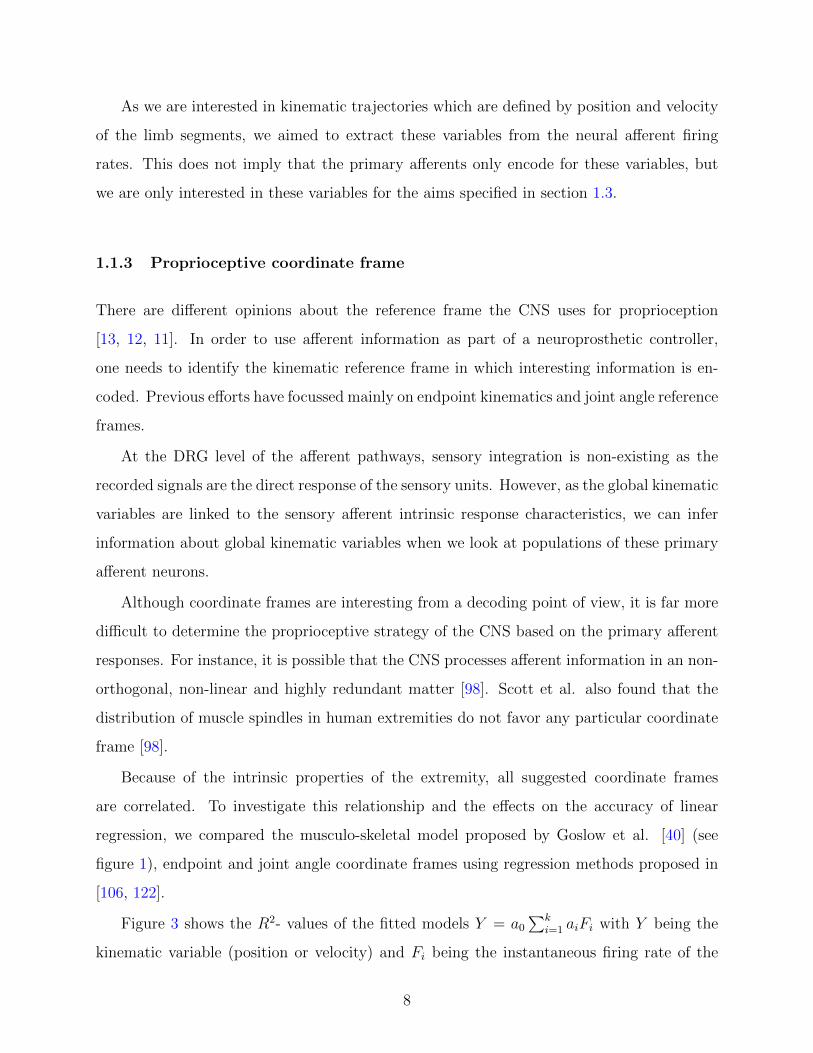
As we are interested in kinematic trajectories which are defined by position and velocity
of the limb segments, we aimed to extract these variables from the neural afferent firing
rates. This does not imply that the primary afferents only encode for these variables, but
we are only interested in these variables for the aims specified in section 1.3.
1.1.3 Proprioceptive coordinate frame
There are different opinions about the reference frame the CNS uses for proprioception
[13, 12, 11]. In order to use afferent information as part of a neuroprosthetic controller,
one needs to identify the kinematic reference frame in which interesting information is en-
coded. Previous efforts have focussed mainly on endpoint kinematics and joint angle reference
frames.
At the DRG level of the afferent pathways, sensory integration is non-existing as the
recorded signals are the direct response of the sensory units. However, as the global kinematic
variables are linked to the sensory afferent intrinsic response characteristics, we can infer
information about global kinematic variables when we look at populations of these primary
afferent neurons.
Although coordinate frames are interesting from a decoding point of view, it is far more
difficult to determine the proprioceptive strategy of the CNS based on the primary afferent
responses. For instance, it is possible that the CNS processes afferent information in an non-
orthogonal, non-linear and highly redundant matter [98]. Scott et al. also found that the
distribution of muscle spindles in human extremities do not favor any particular coordinate
frame [98].
Because of the intrinsic properties of the extremity, all suggested coordinate frames
are correlated. To investigate this relationship and the effects on the accuracy of linear
regression, we compared the musculo-skeletal model proposed by Goslow et al. [40] (see
figure 1), endpoint and joint angle coordinate frames using regression methods proposed in
[106, 122].
Figure 3 shows the R2- values of the fitted models Y = a0∑k
i=1 aiFi with Y being the
kinematic variable (position or velocity) and Fi being the instantaneous firing rate of the
8

i-th afferent neuron (results are based on data from a single animal). See section 2.2.2 for a
detailed description of the method. During a random movement trial (see 3.2.2), kinematics
and neural data were recorded. For each kinematic variable, the neuron with the highest
correlation was selected and the R2-value was found (black bars in figure). Subsequently,
neurons were added to the model as long as each consecutive neuron added > 1% to the R2
value. The number on top of each bar indicates the number of neurons included and the
total length of the bar is the resulting R2-value of the model.
We can see that the same population of neurons can represent kinematic variables in
various coordinate frames and that position tends to be better represented than velocity.
This seems to agree with results presented by Weber in 2007 although these results were
observed during awake behaving animals [123]. Note that we are only looking at linear
models and that we cannot make any conclusions about how the CNS interprets these signals.
Innervating of the muscle spindles by γ-motor neurons have raised various theories about
the coordinate frame that is represented by the firing rates of these neurons. It is widely
accepted that the muscle spindle firing rate is directly correlated by the muscle fiber stretch
and stretch velocity when gamma-motor activation is held constant (see section 1.1.2.1).
However, modulation of the gamma-drive during active movement of the extremity could
potentially result in a reference frame change. Muscle spindle behavior in freely moving
cats have shown large changes in the responsiveness to limb kinematics depending on the
type of movement. This suggests that the fusimotor action can be independently set by
the CNS depending on the motor control task at hand [83]. Therefore, we can deduct that
γ activity is not used to statically transform coordinate systems. This is confirmed by
human microneurography studies that showed that γ-motor neuron activity is modulated by
attention [88, 50]. Ribot-Ciscar et.al. found that when the subject was asked to focus on
the final position in a reach task, the muscle spindle activity increased sensitivity to position
and decreased sensitivity to velocity components [88].
In absence of significant γ fluctuations during motor task, muscle spindles are known
to responds to stretch and stretch-velocity components of muscle. A simulation study was
performed to quantify the ability to infer global kinematic variables from muscle length
information. Thereto, we modeled the muscle lengths as a linear function of global variables
9

0
0.1
0.2
0.3
0.4
0.5
0.6
0.7
0.8
0.9
1R
2 Va
lue
R2
Valu
e
Contribution 1st neuronContribution additional neurons
SSMa
VLIPMG
STSMp
RF
LG-PL
BF YX RTheta
AnkleKneeH
ip
0
0.1
0.2
0.3
0.4
0.5
0.6
0.7
0.8
0.9
1
SSMa
VLIPMG
STSMp
RF
LG-PL
BF YX RTheta
AnkleKneeH
ip
Position
Linear regression of example dataset in different coordinate frames.
Velocity
Figure 3: R2-values indicating the amount of variability explained by the neural data. The
black bars indicate the efficiency of the best neuron, the white bars indicate the efficiency
using multiple neurons. The best n neurons were selected per kinematic variable based on
their added value to the decoded variable.
10

0
0.1
0.2
0.3
0.4
0.5
0.6
0.7
0.8
0.9
1
R2 V
alu
e
Linear relations between muscle space and other coordinate systems
HipKneeAnkle
XY
ThetaR
Joint Angle Polar coord.Cartesian coord.
SSM
a
VL
IPMG
ST
SM
p
RF
LG
-PL
BF
SSM
a
VL
IPMG
ST
SM
p
RF
LG
-PL
BF
SSM
a
VL
IPMG
ST
SM
p
RF
LG
-PL
BF
Figure 4: The goslow muscle model [40] compared to other coordinate frames. A simulation
modeled various global kinematic variables onto the muscle lengths provided by the goslow
model. The R2 value is based on the fitted data of the model.
(joint coordinates, cartesian endpoint coordinates and polar endpoint coordinates). Goslow’s
musculo-skeletal model was used to generate simulated kinematics throughout the range of
motion of the hindlimb of cat [40]. Figure 4 shows the resulting R2 values after fitting each
muscle length as a linear function of the global variables. It is clear that joint angles are
more linearly related to muscle length than endpoint kinematics.
This figure shows that the joint angles are closest related to the muscle length coordinate
frame. If we assume that muscle spindles are primarily responsible for generating proprio-
ception, it is likely that the firing rate of muscle spindles are best modeled with joint angles
as the global kinematic variables. Similar results were shown in Stein et al. 2004 [106].
In summary, suggestions about the implementation of coordinate frames for propriocep-
tion in the CNS has been a topic of discussion over the past 20+ years. It has been shown
that activity in higher areas of the CNS related to motor planning can be describe in terms of
polar coordinates of the endpoint [75, 94, 38]. Although the direct response characteristics of
primary afferents are well documented and thoroughly described (see section 1.1.2), the in-
11

herent kinematic correlations of the extremity result in the ability to infer global kinematics
at the level of the primary afferents. Sensory integration of these signals can further result
in a global representation of limb kinematics in higher regions of the CNS [105, 98, 12, 11].
1.1.4 Role of somatosensory afferents in regulating motor output
As previously mentioned, the exact role of somatosensory afferents in motor control remains
unsolved. However, ever since the discovery of the ‘simple reflex’ by Sherrington in the early
1900’s, is has been clear the somatosensory afferent have a direct impact on motor control.
The increased firing rate of muscle spindles during stimulation of the γ- motor neurons
has resulted in different ideas on the role of sensory integration in motor control [69]. Sev-
eral suggestions were proposed to explain the purpose of the γ drive including the ‘follow-up
length servo’ and the direct servo mechanism. Although these claims have since been dis-
puted, no concluding understanding exists about the strategies underlying the fusimotor
system and γ-motor drive [83, 113].
A relatively recent review on the effects of afferent input in locomotion revealed that
cutaneous afferents as well as muscle afferents influence the locomotion pattern generated
at the spinal cord level [90]. Removing cutaneous inputs from the hindlimb in cat will not
prevent the animal from walking on a treadmill. However, when walking on a horizontal
ladder, the animals were not able to place their feet on the rungs during the first 3-7 weeks
following de-afferenting the extremity. Although the animal regained the ability to perform
this task, the walking behavior never went back to normal [15, 14]. In addition, when
spinalized, the regained walking behavior disappeared and the animals were no longer capable
of correctly placing their paws on the rungs in contrast to spinalized animals with intact
cutaneous afferents. The role of cutaneous afferent input thus appears to be crucial for the
expression of locomotion and recovery of locomotion after spinal cord injury [90].
Proprioceptive control of movement is thought to depend on the co-operation of sensory
neurons from multiple modalities such as muscle spindles, joint and cutaneous afferents [37].
Gandevia et. al. also found evidence that motor commands contribute to proprioception.
In experiments were the subjects were asked to match wrist angle in the absence of vision,
12

they found that the subject perceived movement of the wrist even in the case were the joint-
muscles were paralyzed and anesthetized [36]. It is therefore clear that proprioception and
motor control are tightly interwoven which is reinforced by the knowledge that there are
many connections between motor- and sensory cortex.
1.1.5 The impact of spinal cord injury to primary afferent response
The short and long term effects of spinal cord injury on primary afferent firing rate response
is not well documented although multiple hypotheses have been brought forward over the
years. Muscle spindles are modulated by static an dynamic γ-motor neurons during intact
behavior. Studies in acute decerebrate and spinal cats showed that static and dynamic
gamma drive is still present in the preparations and could be measured independently dur-
ing pharmaceutically induced walking. In both preparations, muscle spindle activity was
increased after onset of the locomotion with a decrease in stretch reflex sensitivity [7]. This
suggests an increase in static gamma drive during walking. There have not been any stud-
ies that have looked at the long term property changes of muscle spindles after spinal cord
injury.
Arutyunyan described muscle spindle response to chronic de-efferentation in 1981 [6]. He
found that the sensitivity of the muscle spindles increase over time and attributes this to
atrophy of the de-efferented muscles. These findings do not necessarily compare to those in
spinal cats. In 1965, Alnaes found that the dynamic fusimotor system is largely driven by
spinal mechanisms initiated by afferent inputs and that the static gamma drive is mediated
by descending tracks from higher brain regions based on dorsal root recordings in spinalized
and decerebrated cats [3].
Spasticity with associated hyper-reflexia is a common complication after spinal cord in-
jury where hyper-reflexia is defined as an increased excitability of the velocity-dependent
stretch reflex. Although it was previously believed that a decreased inhibition of fusimo-
tor drive was inherent to the increase in reflexivity, nowadays, it is thought that different
mechanics, such as recurrent inhibition of motoneurons and/or a reduced presynaptic inhibi-
tion of Ia afferents, are involved in this behavior [76]. Qualitative results of upper extremity
13

spindle responses in unilateral cerebral stroke patients with spasticity seem to confirm these
beliefs. They show no difference in muscle spindle behavior with respect to healthy con-
trol subjects suggesting that the fusimotor system does not contribute significantly to the
hyper-excitability of the stretch reflex [125].
1.2 USING AFFERENT INFORMATION FOR NEURAL PROSTHESES
Neural prostheses relying on neural signals for control require a stable interface with the
nervous system. The type and location of the interface determines the types of signals that
can be processed. This section will discuss some of the uses for afferent neural interfaces and
give a brief summary on currently used electrodes used to interface with the nervous system.
1.2.1 Using primary afferent or external sensors?
For FES-based neural prostheses, one can question whether using afferent information to
infer limb kinematics has sufficient advantages over externally placed sensors that it justifies
the associated invasive surgical procedures. Depending on the application and complexity of
the neural prostheses, the answer might differ. For example, compensating foot-drop during
gait using FES can well be addressed by using a simple foot-switch [22]. However, when we
increase the number of variables we are interested in, using external sensors likely results in
problems with usability and reliability.
Using primary afferent information to decode the limb state can also potentially be favor-
able as the DRG can be used as a centralized access point for recording sensory information
throughout the extremity. The alternative of multiple external sensors is practically difficult
to achieve.It is my opinion that extracting information from primary afferent neural activity
for the use in neural prostheses will provide a better alternative than external sensors for
complex FES-applications.
14
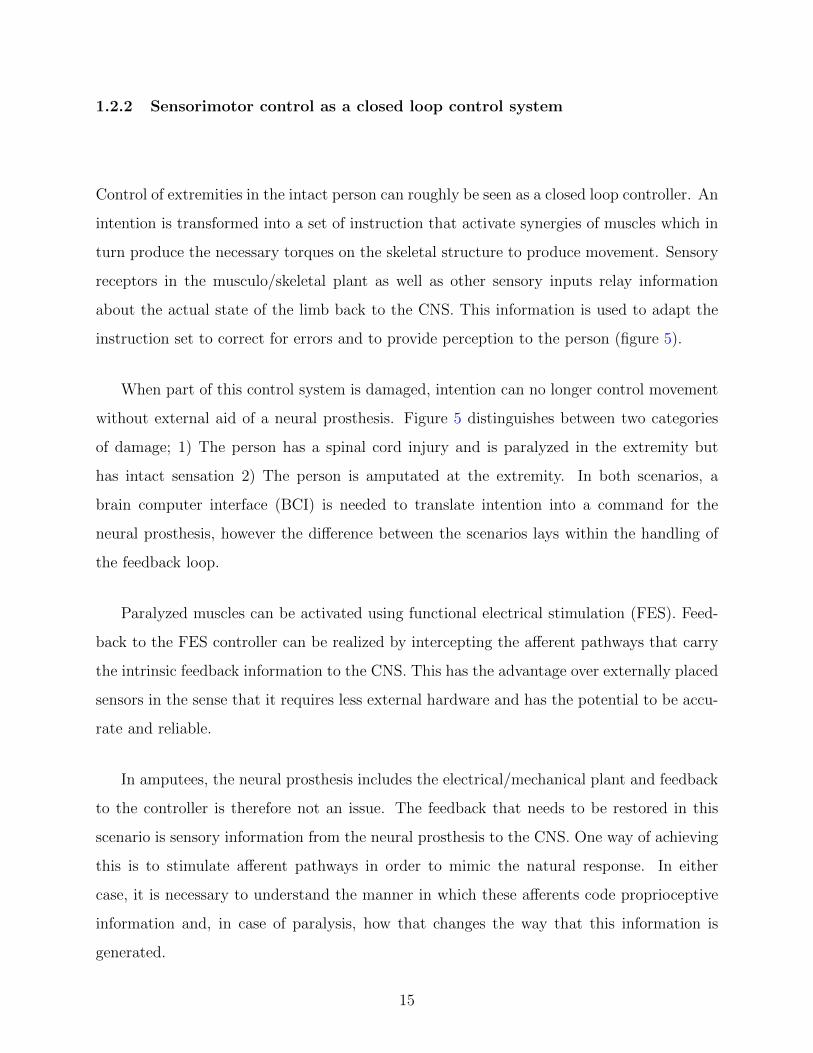
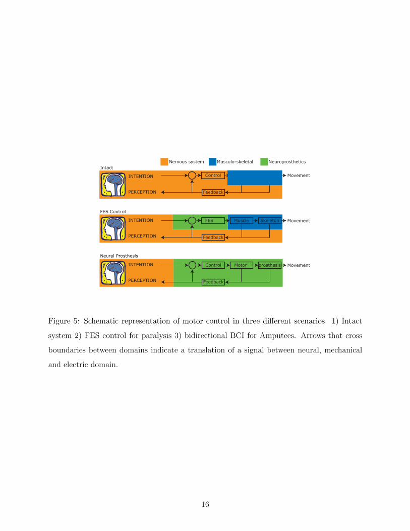
1.2.2 Sensorimotor control as a closed loop control system
Control of extremities in the intact person can roughly be seen as a closed loop controller. An
intention is transformed into a set of instruction that activate synergies of muscles which in
turn produce the necessary torques on the skeletal structure to produce movement. Sensory
receptors in the musculo/skeletal plant as well as other sensory inputs relay information
about the actual state of the limb back to the CNS. This information is used to adapt the
instruction set to correct for errors and to provide perception to the person (figure 5).
When part of this control system is damaged, intention can no longer control movement
without external aid of a neural prosthesis. Figure 5 distinguishes between two categories
of damage; 1) The person has a spinal cord injury and is paralyzed in the extremity but
has intact sensation 2) The person is amputated at the extremity. In both scenarios, a
brain computer interface (BCI) is needed to translate intention into a command for the
neural prosthesis, however the difference between the scenarios lays within the handling of
the feedback loop.
Paralyzed muscles can be activated using functional electrical stimulation (FES). Feed-
back to the FES controller can be realized by intercepting the afferent pathways that carry
the intrinsic feedback information to the CNS. This has the advantage over externally placed
sensors in the sense that it requires less external hardware and has the potential to be accu-
rate and reliable.
In amputees, the neural prosthesis includes the electrical/mechanical plant and feedback
to the controller is therefore not an issue. The feedback that needs to be restored in this
scenario is sensory information from the neural prosthesis to the CNS. One way of achieving
this is to stimulate afferent pathways in order to mimic the natural response. In either
case, it is necessary to understand the manner in which these afferents code proprioceptive
information and, in case of paralysis, how that changes the way that this information is
generated.
15
INTENTION
PERCEPTION
Control Muscle Skeleton
Feedback
FES Muscle Skeleton
Feedback
INTENTION
PERCEPTION
Control Motor prosthesis
Feedback
INTENTION
PERCEPTION
Movement
Movement
Movement
Intact
FES Control
Neural Prosthesis
Nervous system Musculo-skeletal Neuroprosthetics
Figure 5: Schematic representation of motor control in three different scenarios. 1) Intact
system 2) FES control for paralysis 3) bidirectional BCI for Amputees. Arrows that cross
boundaries between domains indicate a translation of a signal between neural, mechanical
and electric domain.
16

1.2.3 Neural interfaces
Electric discharges from muscle tissue and neurons have been recorded since the eighteenth
century [57]. However, not until recently were we able to record from large populations of
neurons simultaneously due to electrode fabrication and signal processing demands. These
developments have enabled neuroscientists to analyze population responses in the nervous
system and advanced the idea of a neuroprosthesis [121, 95]. In this section, the most
commonly used electrode interfaces for neural interfaces are discussed. Because this field is
rapidly expanding and progress is made continuously, I do not pretend, nor strive to include
all actively used electrodes.
In 1992, Jones et al. published a method for manufacturing a glass/silicon composite
intracortical electrode array (Utah-array, Blackrock Microsystems, Utah) which has since
been the standard for microelectrode arrays (MEAs) [55]. Although the array was originally
designed for intracortical recordings, it has been used in numerous studies in different levels
of the nervous system in animal [77, 16, 115, 106] and human [47, 58] subjects. Some of the
current developments using this type of array include new wafer fabrication technologies [8]
and the development of a wireless version of the array [24].
NeuroNexus (Neuronexus technologies, Ann Harbor) has been a very successful spinoff
company from the University of Michigan. They fabricate electrodes based on thin film
MEMS processes which are much cheaper to fabricate than the previously mentioned Utah
array [46, 59]. They typically contain 16-64 electrodes per probe and are better suited for
recording activity at different layers in the brain as the recording sites are located along
the insertion direction. Continuous advances in electrode design are aimed at reducing
tissue encapsulation [100], drug delivery [99], and improvements in biocompatibility using
specialized coatings [27].
17

Microwire arrays, fabricated by TDT (Tucker Davis Technologies, Alachua, USA) and
MircroProbes (MicroProbes for Life Science, Gaithersburg, USA), are the third type of MEAs
currently available and have been used for recording and stimulation studies in both acute
and chronic experiments [99, 124]. Penetrating multi electrode arrays are currently the most
viable and reliable solution for neural prostheses that require high specificity on multiple
channels and are currently used by the Braingate and BrainGate2 projects to interface
cortical areas in human [31, 96].
Intrafascicular electrodes can be used to do multiunit recordings of motor or afferent
information in the peripheral nervous system.[70, 39, 61] In 1996, Yoshida et al. demon-
strated that LIFE electrodes could be used in a closed loop FES system to control ankle
flexion/extension. Here, LIFE electrodes were inserted in the common peroneal nerve and
the tibial nerve to record afferent activity related to the ankle angle while a third LIFE
electrode was placed in a fascicle of the tibial nerve innervating the medial gastrocnemius
muscle for stimulation [132].
Non-penetrating interfaces include EEG, MEG, Nerve cuffs and ECog arrays. Nerve cuffs
have been used for recording and stimulation of peripheral nerves. Haugland used a nerve
cuff to detect the start of the stance phase from the activity of the Sural nerve as a control
for a foot-drop orthosis [45]. Other groups have proposed similar usage of nerve cuffs for
gait detection which are well documented in the 2002 review on portable FES-Based Neural
orthoses by Lyons et al. [65]. As the other interfaces are incapable of being used in the
peripheral nervous system, they will not be discussed in this section.
1.2.4 Inferring limb state from afferent activity
Decoding information from neural populations has been investigated for a long time with,
perhaps, its most appealing example being control of a robotic prosthesis using population
decoding in motor cortex [38]. The work presented in this thesis utilizes an interface with the
nervous system at the level of the DRG. This has three main reasons; 1) All recorded neurons
in the DRG are, by definition, primary afferents 2) There is no integration of neuronal signals
at this level and therefore the spatial/temporal resolution is very high and 3) The DRG are
18
easily accessible. When recording in the DRG, the afferent cell type can easily be classified as
either a muscle spindle, tendon organ or cutaneous. In the proposed project, this information
will be used to increase the accuracy of the prediction of kinematics.
Although a variety of models predict muscle spindle firing rate from the kinematic vari-
ables, it is inherently more difficult to invert these models to predict kinematics. Primary
reasons for this are 1) Non-linear behavior of the muscle spindle and 2) Ambiguity of position
and velocity components of the firing rate. To date, decoding efforts have not attempted
to invert the muscle spindle models but rather have based the decoding on computing a
weighted average of a population of neurons [105, 122, 106]. In this technique, a kinematic
variable (Y) such as extremity endpoint, joint angle or their velocities is modeled by a
weighted average of afferent firing rates (F) (Y = a +∑
i biFi). It was shown that a lim-
ited number of neurons could provide accurate predictions of the kinematic variable. When
decoding velocities, position could be inferred by integrating the output. However, despite
the good predictions, this model fails when it comes to generalizability. When a different
kinematic data set is used to train the model, accuracy quickly diminishes. In addition, the
model tends to overestimate the kinematic variable during higher velocities due to the fact
that the model is trained on a single kinematic parameter. We refer to this approach as
‘reverse’ regression since the natural relationships between the dependent and explanatory
variables are reversed. Chapter 2 and 3 will provide more details on the classification of
‘reverse’-regression as well as indicate some of the problems that occur as a result of this
reversal relationship.
The next two chapters of this thesis propose new decoding methods to extract kinematic
information from primary afferents. These methods consists of modeling the firing rates of
the primary afferents as functions of the kinematic parameters, and inverting these models
via a state-space procedure to decode simultaneously all limb kinematics. Preliminary results
were presented in [119] and an extension of these methods was proposed in Wagenaar et al
(2009). We compared the efficiencies of the resulting estimates with those predicted using
reverse regression [106, 122] and discuss the feasibility of using natural feedback decoding in
neuroprostheses. The results of these studies are described in later chapters of this thesis.
19
Finally, the coordinate frame in which limb kinematics are decoded has typically been
based on polar coordinates of the endpoint of the limb or the individual joint angles [123, 12].
Scott et al. (1994), found no evidence for a particular coordinate frame based on modeling
studies of muscle spindle distributions [98]. Stein et al. (2004), also found no significant
difference in correlation coefficients when comparing PA firing rates to kinematic state in
polar endpoint coordinates and joint angle space [123, 106]. We included both endpoint and
polar coordinates in the analysis of this paper since both representations are relevant for
implementation in neural prostheses. In 1998, Prochazka described the possibility to decode
muscle lengths from primary afferent firing rates by inverting the firing rate models [82].
However, the manuscript does not elaborate on the methods which were used and if these
were actually decoded trajectories from a single or multiple neural responses.
1.2.5 Closed-loop control of FES using natural sensors
In applications where functional electrical stimulation (FES) is used to restore limb functions
such as gait, posture or foot drop, it is important to provide feedback information to the
controller in order to be able to cope with perturbations, muscle fatigue and non-linear
behavior of the effected muscles [67, 126, 123]. Accessing and decoding the activity in native
afferent signaling pathways can be a natural way to determine the kinematic state (i.e.
position and velocity) of the controlled extremity [44]. Feasibility of this approach has been
demonstrated by controlling the ankle angle in a closed loop controller using the compound
afferent input recorded from LIFE electrodes by Yoshida [131]. Micera et al. used nerve
cuffs, implanted around the Peroneal and Tibial nerve ,to infer ankle angle estimates using
neuro-fuzzy network decoding algorithms [71].
The methods used by Yoshida and Micera predicted a continuous representation of a
single kinematic variable from the neural data. Although this might be sufficient for simple
closed loop FES controllers, it is likely not specific enough for a complete neural prosthesis.
For continuous predictions of multiple variable relating to the kinematic state of the ex-
tremity, one needs to record from a larger and more diverse population of primary afferents
to attain a more complete estimate of limb state. One solution is to record at the dorsal
20
root ganglia where all proprioceptive information converges into the central nervous system.
Recording at this site with multi-electrode arrays grants access to a wide variety of state
information distributed across many individual neurons [106, 122, 123].
Instead of a continuous representation of limb kinematics, one could implement closed
loop control using an event based classification system as suggested by Borisoff et al. [10].
Although this work was triggered by closed loop FES for bladder control [54], it could
easily be extended to specific kinematics states of the extremity. Using classifiers instead
of continuous estimates of limb state could provide a couple of advantages. In example,
if stimulation parameters for FES should be changed depending on a certain threshold in
the limb kinematics, classifiers might be better predictors of this threshold than continuous
decoders. Section 6.2 of this thesis will elaborate a little further on the use of classifiers for
closed loop FES systems. The rest of this thesis is focussed on continuous decoding of limb
kinematics and the use of firing rate models to infer these variables.
In summary, it is widely recognized that a FES system would benefit tremendously from
sensory feedback in terms of adaptability and functionality as long as the feedback system
would be reliable [79, 67]. Using closed loop control of FES, it is possible to change the
stimulation parameters dynamically depending on the feedback from the sensors. When
accurate predictions of limb state are available to the FES controller, it will be able to
compensate for muscle fatigue and external perturbations.
1.3 SPECIFIC AIMS
This section describes the specific aims addressed in this manuscript. Each specific aim is
discussed in a separate chapter following this introduction.
1.3.1 Direct decoding of primary afferent neuron firing rates
In this aim, we propose a new method for decoding primary afferents by modeling the
firing rate of each recorded neuron to infer limb state variables. We hypothesize that direct
21

regression will improve the decoded trajectories as it correctly models the observed firing
rates and can take into account the multivariate response of an individual neuron.
• Hypothesis: Direct regression using non-linear firing rate models improves limb kinematic
estimates over currently used reverse regression methods.
1.3.2 State-space decoding of primary afferent neuron firing rates
The previous aim confirmed the fact that it is possible to estimate limb position from afferent
recordings using direct linear regression techniques. However, the dynamic muscle spindle
response mediated by limb velocity is not incorporated in those linear models. The focus of
this SA is to develop non-linear models to include both position and velocity information
from muscle spindles to resolve the ambiguity of position and velocity contributions in the
afferent firing rate models. In addition, contrary to currently used decoding algorithms, the
decoding models will be able to predict multiple kinematic parameters, such as joint angles,
simultaneously, thus finding the best prediction of the limb kinematics rather than treating
each variable as independent.
• Hypothesis 1: State-space decoding will be able to take into account the kinematic
constraints of the extremity and improve decoding accuracy using this information.
• Hypothesis 2: Including the derivatives of the kinematic variables to the firing rate
models will result in more accurate predictions of limb kinematics.
1.3.3 Improved decoding techniques for realtime applications.
In order to utilize the decoding techniques in a realtime FES application, non-linear models
will be implemented in a real-time setup which will enable the use of these decoding tech-
niques in a neural prosthesis environment. Although the decoding methods described in the
previous specific aims produce accurate results, the decoding speed is insufficient for any
realtime application. In this specific aim, non linear methods are described that are capable
of predicting limb kinematics in ‘real-time’.
22

• Hypothesis: Alternative methods using non-linear reverse regression methods can im-
prove limb kinematic decoding accuracy while continue to be able to be implemented in
a ‘real-time’ environment.
1.3.4 Closed loop FES using primary afferent response as feedback
Mechanical sensors have proven difficult to implement in prostheses due to their unreliability,
fragility and other practical difficulties. Most FES systems use open-loop controllers as a
result of these limitations. However, a closed-loop feedback controller will increase the
adaptability and stability of the FES system. Specific Aim 4 will focus on developing a
controller for FES-evoked closed-loop walking. This will be implemented using a finite state
controller, alternating between states based on the estimated limb state as provided by the
neural decoder. By closing the loop, we hypothesize that the controller will be able to
generate reliable walking behavior under various conditions.
• Hypothesis 1: Primary afferent firing rates can be used to predict limb kinematics during
functional electrical stimulation.
• Hypothesis 2: Estimates of limb state can be used to control functional electrical stimu-
lation in a closed loop state feedback mechanism.
23

2.0 IMPROVED DECODING OF LIMB-STATE FEEDBACK FROM
NATURAL SENSORS
The contents of this chapter are published as: “Improved decoding of limb-state feedback
from natural sensors” which was published in Conf Proc IEEE Eng Med Biol Soc, 1:42069,
2009, c©[2009] IEEE [119]. It covers specific aim 1 of this thesis and describes an alternative
to previously suggested methods for decoding limb kinematics from primary afferent firing
rates.
2.1 INTRODUCTION
During movement, proprioceptors constantly assess and relay sensory information about
the physical state of the peripheral musculature to the central nervous system (CNS). This
feedback allows the CNS an indication of the actual state of the limb and consequently
to adapt motor drive in order to realize stable and efficient movements. When functional
electrical stimulation (FES) is used to restore action to paralyzed limbs, a similar feedback
mechanism is required for executing complex movements and adapt for perturbations or
fatigue of the muscles. Accessing and decoding the activity in native afferent signaling
pathways would be a natural way to determine the kinematic state (i.e. position and velocity)
of the controlled extremity [131]. Our initial goal is therefore to predict/decode the kinematic
state of the leg using the ensemble activity of primary afferent neurons, recorded with arrays
of penetrating micro-electrodes in the dorsal root ganglia (DRG).
Previously, reverse regression methods were used to estimate limb kinematics from en-
sembles of simultaneously recorded primary afferent neurons in the dorsal root ganglia of
24

anesthetized [106] and alert, locomoting cats [123]. However, direct regression methods are
more efficient and flexible than reverse regression approaches. Direct regression methods
include population vectors [38], optimal linear estimators [92], maximum likelihood [20],
Bayesian [93] methods, and filtering/dynamic Bayesian methods [133]. See [19] for a re-
view and references therein. Our goal for this paper is to determine if the simplest likelihood
method can improve upon reverse regression to decode limb position from the spiking activity
of a small ensemble of primary afferent neurons.
2.2 METHODS AND DATA
2.2.1 The experiment
Center-out patterns in a 2-dimensional plane were imposed on the hind limb of an anes-
thetized cat by a robotic arm (figure 6:b). These movements spanned a significant part of
the range of motion for the limb. See Stein et al. [106] for complete details.
The ankle (A1), knee (A2), and hip (A3) angles of the hind leg were recorded at 120
Hz with a high speed video capture system using markers placed at the Iliac Crest (IC),
Hip, Knee, Ankle and Metatarsophalangeal (MTP) joints (figure 6:c). Figure 7 shows the
recorded joint angles of knee and ankle as functions of experimental time during one trial of
the experiment. The trials were repeated to create separate data sets for model fitting (i.e.
encoding) and testing (i.e. decoding).
Primary afferent neurons were recorded using penetrating microelectrode arrays with 50
and 40 electrode sites (5x10 and 4x10, 400µm spacing). The arrays were inserted in the L7
and L6 dorsal root ganglion using a high velocity inserter. The neural signals were acquired
with a sampling frequency of 30 kHz and bandpass filtered with cutoff frequencies of 100Hz
- 3000Hz. Spikes were sorted offline via cluster analysis; figure 6:a shows the raster plot of
the spike trains of 15 neurons. We then smoothed the spike trains using a one-sided normal
distribution kernel with SD 0.15 sec. We denote by FRi the resulting firing rate of neuron i.
25

100 50 0 50 100 150
200
150
100
50
0
Hindlimb Kinematics
IC Hip
Knee
AnkleMTP
Joint anglesLimb segments Joint markers
-240 -200 -160
50
10
01
50
Center-out Movement
x(mm)
y(m
m)
10 20 30 40 50 60 70 80 900
5
10
15
Time (s)
Ne
uro
n N
r.
x(mm)
y(m
m)
Primary afferent responsesa)
c)b)
Figure 6: c©[2009] IEEE, a) Responses of different neurons to passive movement of the
leg. Each vertical line represents an action potential. b) The endpoint kinematics of the
hindlimb during passive center-out movement. This movement is imposed on the hindlimb
using a robotic manipulator. c) Schematic of the hindlimb; joint angles are being decoded
to represent the kinematic state of the limb.
26

2.2.2 Reverse regression
Reverse regression/correlation was used previously to estimate angular positions and veloci-
ties for the hip, knee, and ankle joints [122, 106]. The “reverse” describes the reversal of the
natural roles played by the stimulus and spike-activity response. Although in reality, it is the
neural activity that varies as a function of joint angular position, reverse regression treats
the firing rates as if they were the inputs (the x’s in regression notation), while the joint
angles are considered the output (the Y variable). That is, the joint angles Ak, k = 1, 2, 3,
are expressed as
Ak = βk0 +∑i∈Sk
βkiFRi (2.1)
where FRi is the firing rate of neuron i, and Sk indexes the set of neurons whose firing rates
correlate most strongly with Ak [106]. Then given a training set of angles and firing-rate
combinations, one computes the usual least-squares estimates β of the β’s; this step is usually
referred to as encoding. In the decoding stage, given the firing rates FR∗i of all neurons in
a small window of time, the predictor of joint angle k is then
A∗k = βk0 +∑i∈Sk
βkiFR∗i
To allow for the possibility that the relationships between neurons’ firing rates and joint
angles are not linear, we will consider in place of Eq.2.1 the more flexible non-parametric
generalization
A = β0 +N∑i=1
si(FRi)
where the si(.) are taken to be moving lines with 4 non-parametric degrees of freedom (DOF).
2.2.3 Direct regression methods
Direct regression methods include population vectors, optimal linear decoding, as well as
likelihood-based and dynamic decoding. Firing rates are considered random variables whose
27

distributions, often just the means, vary with joint angles. Assuming that firing rates are ap-
proximately normal with constant variances σ2i , the simplest relationship one could consider
for neuron i is
FRi = α0i + α1iA1 + α2iA2 + α3iA3 + σ2i εi, (2.2)
i = 1, . . . , N , where εi are standard normal random errors. Note that Eq. 2.2 specifies one
relationship per neuron, whereas Eq. 2.1 specifies one relationship per angle. Then given
a training set of angles and firing-rate combinations, encoding consists of computing the
maximum likelihood/least-squares estimates of the αji and σ2i . In the decoding stage, the
observed firing rates FR∗i of all neurons in a small window of time are each assumed to
have distributions specified by Eq. 2.2, where the αji and σ2i are now taken to be equal to
their estimates from encoding. The predictor of joint angle is then the least square/maximum
likelihood estimate of (A1, A2, A3) obtained from the set of N models in Eq. 2.2, i = 1, . . . , N .
Eq. 2.2 is the simplest firing rate model we could consider. To allow for non-linear
relationships between firing rates and angles, we will instead use sji(Aj) in place of αjiAj,
j = 1, 2, 3, where sji(.) are splines with 4 non-param. DOF. Our model will also include
interactions between pairs of joint angles, to allow for the possibility that relationships
between firing rates and a particular angle vary with another angle. The data supports
this possibility, as illustrated by Figure 8. We also considered hind limb biomechanics and
physiology to guide our choice of physiologically plausible firing rate models: muscle afferents
(i.e. primary and secondary muscle spindles, tendon organs) encode maximally two out of
the three joint angles (bi-articulate muscles span either hip/knee or knee/ankle). Therefore,
each neuron is modeled to encode either for one angle (hip, ankle or knee), or for two angles
(hip and knee or ankle and knee). That is, for each neuron i, we considered the two families
of firing rate models
FRi = α0i + sji(Aj) + ski(Ak) + sji(Aj) : ski(Ak) + σ2i εi, (2.3)
for j, k = 1, 2 (ankle/knee) and j, k = 2, 3 (knee/hip), where sji(Aj) : ski(Ak) denotes an
interaction between angles j and k, and within these two families of models, we determined
the statistical significance of each term using the Bayesian information criterion (BIC) and
selected the best model based on this measure.
28

2.2.4 Contrasting methods
Direct regression offers several theoretical advantages over reverse regression. In direct re-
gression, all angles are allowed to contribute to explaining the firing rates of each neuron,
whereas in reverse correlation, angles are each decoded separately, using different groups of
neurons. From a physiological view point, direct regression is more appropriate because Eq.
2.2 attempts to model how each neuron encodes joint angles, whereas there is no physiological
basis for Eq.2.1.
From an efficiency view point, if all neurons encoded single joint-angles, both methods
should predict approximately similar trajectories. As most muscles span multiple joints,
responses from muscle afferents code for multiple angles simultaneously. Fig. 8 shows an
example of a neuron whose firing rate depends not only on the hip angle but also on the knee
angle. Reverse regression decodes each angle separately so it cannot properly extract the
information in firing rates about several angles. In contrast, direct regression makes efficient
use of this information provided the firing rate model in Eq. 2.3 is accurate. For example, if
one of the joint angles is consistently better represented in the afferent data set, the weaker
contributor will be poorly estimated by a reverse regression method. On the other hand,
direct regression combines the information of strongly and weakly encoded angles to improve
the prediction of both.
2.3 RESULTS
We first selected the best 25 neurons, encoded using the first center-out movement sequence
of the experiment, and decoded with the second center-out movement trial. Fig. 7 shows
true knee and ankle trajectories, along with the decoded trajectories using reverse and direct
regression. Ankle and hip angles gave similar results so we do not show the latter. The two
decoding methods produce visually comparable results.
The integrated squared error (ISE) provides a more quantitative assessment of efficiency.
For a particular data set, the ISE is the squared difference between the decoded and actual
29

40
60
80
100
Decoding Limb Kinematics using 25 Neurons
Knee A
ngle
(deg)
0 5 10 15 20 25 30
20
40
60
80
100
Time (sec)
Ankle
Angle
(deg)
Ankle Angle
Old Method
New Method
Figure 7: c©[2009] IEEE, True knee and ankle trajectories (solid thin curves), along with
decoded trajectories using reverse regression (dashed) and direct regression (solid). Decoded
trajectories are based on the best 25 neurons.
30

trajectories, integrated over all time bins. For this particular experiment, the time bins cor-
responding to the rest position account for over half of all bins. We therefore downweighted
these bins so that their contribution would be comparable to the contribution of each of the
8 angle configurations. The ISE is a useful efficiency measure because it typically decreases
proportionally to the inverse of the number of neurons. Therefore, based on this measure,
the accuracy of a method based on N1 neurons will be comparable to the accuracy of another
method based on N2 neurons when N2 = N1 ×R, where R = ISE1/ISE2 is the ratio of the
ISEs of the two methods.
The ISE ratios for knee and ankle in Fig. 7 are 1.12 and 0.97 respectively which indicates
both methods are approximately equally efficient. This is somewhat surprising because most
neurons actually encode more than one joint angle. Indeed, when we consider Figure 8, which
shows the firing rate of a typical neuron versus hip angle: the relationship is not random,
which suggests that this neuron encodes for hip angle. Note also that the + and o plotting
symbols correspond to small and large knee angles respectively: the two sets of symbols
hardly overlap, which suggest that the neuron also encode information about knee angle.
Moreover, the relationship between firing rate and hip angle varies with knee angle, which
suggests an interaction between hip and knee angles. These characteristics are common to
most afferent neurons we examined.
Because direct regression models how each neuron encodes information about joint an-
gles, it makes better use of the information about angles in the neurons’ firing rates. The
comparatively good efficiency of reverse regression might be due to robustness against model
misspecifications: while reverse regression uses one model per angle, direct regression speci-
fies a different model for each neuron, so that even minor model misspecifications can add up
across neurons. It also might be attributed to the number of neurons used and the careful se-
lection of the neurons used to predict limb kinematics. The results in Fig. 7 used 25 neurons
from 2 recording sites. We are unlikely to have that many well defined neurons in practice,
so we are interested in the performance of the two methods given neuron populations of
different sizes.
Fig 9 shows the result of the following analysis. We first selected a pool of neurons
encoding “well” for knee and ankle angles: we regressed the firing rates of all neurons on a
31

70 75 80 85
010
20
30
40
50
60
Afferent Response to Hip and Knee Angle
Hip Angle (deg)
Firin
g R
ate
(H
z)
Small Knee Angles (<60 deg)
Large Knee Angles (>75 deg)
Figure 8: c©[2009] IEEE, Firing rate of a typical neuron varies with hip angle, in response to
passive movement of the leg. The + and o plotting symbols correspond to large and small
knee angles resp. A spline was fitted through each of the two subsets and is plotted as a
dashed line. The clear separation between the lines indicate that the neuron encodes for
knee angle as well as hip angle.
32

smooth function of knee and ankle angles, and retained only the neurons for which the two
angles explained more than 40% of firing rate variations. We thus retained 64 of the 153 total
neurons. We then selected m neurons at random out of this pool of 64 neurons, decoded
knee and ankle trajectories using these m neurons using reverse and direct regression, and
calculated the ISE ratio of the two methods. We repeated this 99 more times to obtain 100
ISE values, which we plotted versus m as a violin in Fig. 9. We repeated this simulation for
several values of m.
Direct regression has clear advantages over the inverse regression methods for all number
of included neurons for the knee and up to 20 neurons for the ankle. This agrees with the
fact that most neurons primarily encode ankle angle and that only direct regression can
extract knee information from those neurons. However, when using higher neuron counts,
the sensitivity of the direct regression approach to inaccuracies in the individual firing rate
models becomes problematic, giving reverse regression methods an advantage.
2.4 DISCUSSION
The results show that direct regression methods are more efficient in using all information
from afferent firing rates which is predominantly due to the ability to include multiple joint
angles in a single model. Being more efficient, this method requires fewer neurons to predict
limb kinematics accurately. Although the CNS might not be sensitive to confounding in-
formation due to the large redundancy in the primary afferent population, the implications
are more severe for neuroprosthetics which have access to a limited subset of the neural
population. For practical reasons, it is desirable to use a decoding method that extracts the
information as efficiently as possible.
Reverse regression treats each kinematic parameter as an independent decoding problem
and will therefore suffer due to confounded information. The ability of direct regression to
use this information results in a better effective use of the afferents predominantly in the
kinematic variables that are poorly represented in the neural population (i.e. A2).
33

5010
015
020
0
Methods comparison
ISE
(rev
erse
reg
ress
ion)
/ IS
E(d
irect
reg
resi
son)
(%
)
0 5 10 15 20 25 30
5010
015
020
0 Knee
Nr. of Neurons
Ankle
ISE
(rev
erse
reg
ress
ion)
/ IS
E(d
irect
reg
resi
son)
(%
)
Figure 9: c©[2009] IEEE, Violin plots of 100 ISE ratios for several neuron population size
m. The mark at the center is at the median. Violin plots are similar to boxplots but they
provide more information: they show the full smooth histogram of the data (here the 100
ISEs) whereas boxplots would only show quartiles and outliers. Independent of the available
neural population, reverse regression would need approx 25% more neurons to be as efficient
as direct regression to decode knee angle.
34

The direct regression method also truly models the stimulus-response encoding proper-
ties of each neuron. In contrast to reverse regression, where model coefficients are arbitrary,
direct regression coefficients convey information to what is encoded by each individual neu-
ron. Insight into what the neurons encode is therefore apparent from the fitted models.
Classification of the origin of a particular neuron can theoretically be extracted from the
model parameters. Although, as noted in the results section, model selection should include
more complex and afferent modality specific models to predict neural type accurately.
Because of its flexibility, it is possible to improve the estimate accuracy by improving
the firing rate models. Although a basic model was chosen to demonstrate the possibilities
in this paper, there are several more sophisticated models of muscle spindles suggested in
the literature. [82, 73, 72] Any of those models can theoretically be implemented using
direct regression methods and will contribute to the prediction accuracy. Fig. 7 shows large
overshoots during the reaching movements. It is believed that the dynamic component of
primary muscle spindles is one of the leading causes for this behavior. Including a velocity
component is only possible when decoding using direct regression methods and will likely
improve the accuracy of the estimated kinematic limb state.
35
3.0 STATE-SPACE DECODING OF PRIMARY AFFERENT FIRING
RATES
As a natural extension of the paper discussed in the previous chapter, the following paper
was published in the Journal of Neural Engineering with the title: “State-space decoding
of primary afferent neuron firing rates” and is included integrally in this chapter with the
permission of IOPScience [120]. It reflects the goals outlined in specific aim 2. Correlations
between the kinematic variables were addressed using a state-space model of the system
and derivatives of the kinematic variables were included in the neural firing rate models to
improve decoding accuracy.
3.1 INTRODUCTION
Proprioception, or the sensation of movement and position, results from the integration of
afferent inputs in the central nervous system (CNS). It provides vital information about the
state of the limb during movement and serves as feedback during motor control to create
stable and accurate movements. In applications where functional electrical stimulation (FES)
is used to restore limb functions such as gait, posture or foot drop, it is important to be
able to include feedback information to be able to cope with perturbations, muscle fatigue
and non-linear behavior of the effected muscles [67, 126, 123]. Accessing and decoding
the activity in native afferent signaling pathways would be a natural way to determine the
kinematic state (i.e. position and velocity) of the controlled extremity [44]. Feasibility of this
approach has been demonstrated by controlling the ankle angle in a closed loop controller
36

using the compound afferent input recorded from LIFE electrodes by Yoshida [131]. However,
a larger and more diverse population of primary afferent recordings is needed to attain a
more complete estimate of limb state. One solution is to record at the dorsal root ganglia
where all proprioceptive information converges into the central nervous system. Recording
at this site with multi-electrode arrays grants access to a wide variety of state information
distributed across many individual neurons [106, 122, 123].
Although it is generally accepted that proprioception is evoked by a variety of primary
afferent (PA) inputs, including muscle, cutaneous, and joint receptors, the muscle spindle
afferents are believed to be the main contributor [35]. Various models with increasing com-
plexity have been proposed for the muscle spindle firing rate [68, 80, 82, 72]. These models
are able to provide accurate predictions of spindle firing rates as a function of muscle length
and presumed gamma drive inputs. While it might be desirable to invert these models to
decode muscle length or limb-state from the firing rates of muscle spindles, such an inversion
is not trivial because the models are non-linear, and position and velocity components of
the firing rate are confounded. Similar limitations are applicable for including cutaneous
afferents as they are often related to limb kinematics in a non-linear fashion.
To date, decoding efforts have avoided these difficulties by directly modeling each of
several kinematic variables as independent functions of the afferent firing rates [106, 122].
These studies used separate regression models to estimate the kinematic state of the hind
limb as a weighted sum of the firing rates in a population of PA neurons recorded in the
dorsal root ganglia (DRG) of cats during passive and active movements. In this paper,
we refer to this approach as reverse regression since the natural relationships between the
dependent and explanatory variables are reversed. We will discuss the limitations of that
approach and propose an alternative decoding approach that does have these limitations.
This method consists of modeling the firing rates of the primary afferents as functions of
the kinematic parameters, and inverting these models via a state-space procedure to decode
simultaneously all limb kinematics. Preliminary results were presented in [119]. In this
paper, we extend the methods proposed in Wagenaar et al (2009) to include time-derivatives
of the kinematic variables (velocities) and allow for decoding multiple correlated kinematic
37

variables. We compare the efficiencies of the resulting estimates with those predicted using
reverse regression [106, 122] and discuss the feasibility of using natural feedback decoding in
neuroprostheses.
Finally, the coordinate frame in which limb kinematics are decoded has typically been
based on polar coordinates of the endpoint of the limb or the individual joint angles [123, 12].
Scott et al. (1994), found no evidence for a particular coordinate frame based on modeling
studies of muscle spindle distributions [98]. Stein et al. (2004), also found no significant
difference in correlation coefficients when comparing PA firing rates to kinematic state in
polar endpoint coordinates and joint angle space [123, 106]. We included both endpoint and
polar coordinates in the analysis of this paper since both representations are relevant for
implementation in neural prostheses.
3.2 METHODS AND DATA
3.2.1 Surgical procedures
All procedures were approved by the Institutional Animal Care and Use Committee of the
University of Pittsburgh. Two animals were used in these procedures. Both were anes-
thetized with isoflurane (1-2%) throughout the experiment. Temperature, end tidal CO2,
heart rate, blood pressure, and oxygen saturation were monitored continuously during the
experiments and maintained within normal ranges. Intravenous catheters were placed in the
forelimbs to deliver fluids and administer drugs. A laminectomy was performed to expose
the L6 and L7 dorsal root ganglia on the left side. At the conclusion of the experiments, the
animals were euthanized with KCL (120 mg/kg) injected IV.
3.2.2 The experiment
A custom frame was designed to support the cat’s torso, spine, and pelvis while allowing the
hind limb to move freely through its full range of motion (figure 10). A stereotaxic frame and
38

RZ-2Neural Data Acquisition System
Markers
Stereotaxic head frame not shown
Electrodes
L6 & L7 dorsal root ganglia
Robot
Figure 10: The animal was positioned in a custom designed frame to support the torso
and pelvis, enabling unrestrained movement of the left hind limb. The foot was attached
to a robotic arm and active markers were placed on the hind limb to track the hind limb
kinematics. A 90 channel micro-electrode array was inserted in the L6/L7 DRG and the
neural activity was recorded using a programmable real-time signal processing system (TDT
RZ2).
39

vertebrae-clamp were used to support of the head and torso, and bone screws were placed
bilaterally in the iliac crests to tether the pelvis with stainless steel wire (not shown in figure
10).
Hind limb kinematics were recorded with a high speed motion capture system (Impulse
system, PhaseSpace Motion Capture, USA). Active LED markers were placed on the iliac
crest (IC), hip, knee, ankle, and metatarsophalangeal (MTP) joints. During post-experiment
analysis, the knee position was inferred from the femur and shank segment lengths and the
hip and ankle markers because skin slip at the knee marker rendered position tracking based
on the knee marker unreliable [106, 122]. Synchronization between neural and kinematic data
was ensured by recording a time-stamp in the neural recording system for every captured
kinematic frame.
A robotic arm (VS6556E, DENSO Robotics, USA ) was used to move the left foot in
the parasagittal plane. The foot was strapped in a custom holder attached to the robot
via a pivoting joint that allowed free rotation of the foot in the parasagittal plane (figure
10). The robot was programmed to generate center-out and random movement patterns
occupying most of the motion range for the foot. Center-out patterns were ramp and hold
displacements of 4cm in eight directions from a center position. Random movements, de-
fined by a uniform distribution of limb positions and velocities within the workspace, were
approximated by manually manipulating the hind limb through the entire workspace over
a period of 5 minutes. During this time, cameras recorded the trajectory and programmed
the robotic manipulator to mimic this trajectory. The robot was then used to manipulate
the hind limb during the remainder of the trials. This ensured that we could generate the
same random movement in a reliable fashion and optimally use the entire workspace of the
hind limb.
Penetrating microelectrode arrays (1.5mm length, Blackrock Microsystems LLC, USA)
were inserted in the L7 (50 electrodes in 10x5 grid) and L6 (40 electrodes in 10x4 grid)
dorsal root ganglia. The neural data was sampled at 25kHz using an RZ-2 real-time signal
processing system from Tucker Davis Technologies, USA. The neural data was band-pass
filtered between 300 and 3000 Hz. A threshold was manually determined for each channel and
40

spike events were defined as each instance the signal exceeded this threshold. Spike waveform
snippets, 32 samples in length (1.2ms) were stored each time a spike event occurred, resulting
in a time series of spikes and their corresponding waveforms per channel. Spike waveforms
were sorted manually during the post-experiment analysis (Offline Sorter, TDT, Inc.).
3.2.3 Current decoding paradigm: reverse regression
Let X = (Xk, k = 1, . . . , K) be the vector of K kinematic variables we want to decode,
based on the firing rates FR = (FRi, i = 1, . . . , I) of I neurons. In this paper, X is the limb
state expressed in one of two different reference frames, a joint-based frame with state vector
(Ak, k = 1, 2, 3) that represents intersegmental angles for the hip, knee, and ankle joints, and
an endpoint frame with state vector (R, θ) that represents the toe position relative to the hip
in polar coordinates. We let X = (Xk, k = 1, . . . , K) denote the velocities of the kinematic
variables, and Z = (X, X) the combined vector of limb kinematics and their velocities. A
subscript t added to any variable means that we consider the value of that variable at time
t. The methodologies described below can be applied to firing rates FR that are either
raw or smoothed spike counts. Here, we computed smoothed instantaneous firing rates by
convolving the spike events with a one-sided Gaussian kernel (σ = 50ms) to ensure causality
[106].
Reverse regression consists of modeling the mean of each kinematic variable Xk as a
function of the spike-activity,
E(Xk) = fk(FR), k = 1, . . . , K, (3.1)
where fk is some function deemed appropriate, for example a linear function as in (3.3).
An estimate fk of fk is obtained by least squares or maximum likelihood regression using
a training set of simultaneously recorded values of X and FR. Then, given the observed
neurons’ firing rates FRobst at time t, the prediction of Xk at t is
X∗kt = fk(FRobst ), k = 1, . . . , K. (3.2)
41

The resulting decoded trajectories {X∗kt, t = 1, 2, . . .}, k = 1, . . . , K, are typically much more
variable than a natural movement, so they are often smoothed to fall within the expected
response frequencies (typically < 20 Hz).
Reverse regression was used by [122] and [106] to predict joint and endpoint kinematics.
They took fk in (3.1) to be a linear function of spike activity, so that
Xk = βk0 +∑i∈Sk
βkiFRi + εk, (3.3)
where Sk indexes the set of neurons whose firing rates correlate most strongly with Xk [106],
and εk are uncorrelated random errors. We adopt the same approach with our data: we
apply reverse regression with the linear model in (3.3) to decode joint angles (Ak, k = 1, 2, 3)
and limb end point position (R, θ), and smooth the decoded trajectories by convolving the
result with a gaussian kernel (σ = 75ms) to improve the decoding results.
One advantage of reverse regression is its simplicity: kinematic variables Xk are de-
coded separately and require just one equation each. However, the method does not allow
physiologically meaningful modeling of the relationships between firing rates and kinematic
variables. Indeed, not only do neurons often encode several kinematic variables simultane-
ously, the manner in which they encode these variables is not necessarily linear or additive.
For example, many muscles in the hind limb span two joints, so that PA neurons code for
multiple joint angles simultaneously. Such a neuron was shown in [119]: its firing rate de-
pended both on ankle and knee angles, the relationship between firing rate and ankle angle
was clearly non-linear, and the relationship changed for different values of knee angle, which
suggested the existence of an interaction between the two joint angles. Such effects cannot
be modeled in reverse regression. It is also possible for neurons to encode not only for kine-
matic variables but also for their derivatives; muscle spindle primary afferents (Ia) are such
neurons. In that case it is possible to decode Xkt based on the relationship between its ve-
locity Xkt ≈ (Xkt −Xk(t−δt))/δt and the neurons’ firing rates, by applying reverse regression
with Xk replaced by Xk in equations (3.1) and (3.2). Based on a linear function fk, this
prediction is
X∗kt = X∗k(t−δt) + δt
(αk0 +
∑i∈Sk
αkiFRobsit
), (3.4)
42

which is different than predicting X∗kt from (3.3). Stein et al (2004) offered an ad-hoc method
of combining these two predictions. However, because it is not motivated by a principle that
guarantees superior results over either separate predictions, we did not consider this method
for our data.
3.2.4 Firing rate models and likelihood decoding
Reverse regression is easy to apply, but it does not make efficient use of the information in
the data since effects such as interactions or effects of derivatives cannot be accounted for.
In contrast, a likelihood approach can account for such effects, and is further known to be
efficient when the models involved are appropriate [56].
The likelihood approach is based on models that describe the physiological dependencies
of firing rates on limb state, which restores the natural relationship between Xk and FRi
that are swapped in the reverse regression approach. That is, the mean firing rates FRi of
each neuron are now modeled as functions of the kinematic variables Z = (X, X),
E(FRi) = gi(Z), i = 1, . . . I, (3.5)
where the functions gi are selected to accommodate any suspected effects between covariates,
such as interactions. Sections 3.2.4.1 and 3.2.4.2 summarize the functions gi we considered
for our data. Although we could let gi also depend on higher order derivatives of X, such
as acceleration, we did not consider that option because PA neurons are known to encode
primarily for muscle lengths and their velocities [85, 64, 72], and previous work using re-
verse regression methods failed to generate accurate estimates of acceleration [123]. The
maximum likelihood estimates gi of gi, i = 1, . . . , I, are obtained based on a training set
of simultaneously recorded values of Z and FR, and on an assumed distribution for FRi.
Here we used the Gaussian distribution since FRi are smooth firing rates, but the Bernoulli
or Poisson distributions could be used instead if FRi were raw spike trains (i.e. unfiltered
spike counts). Then, given the observed firing rates FRobst at time t, the prediction of Z is
obtained by solving the system of I equations
FRobsit = gi(Z
∗t ) + εit, i = 1, . . . I (3.6)
43

for Z∗t . Note that all components of Z are decoded simultaneously, whereas they are decoded
separately in reverse regression. When the firing rates are not modulated by the velocities,
so that the gi’s are functions only of X, solving (3.6) amounts to performing standard least
square estimation when the gi’s are linear functions of their inputs; see section 3.2.8. Oth-
erwise, it can be challenging. In particular, (3.6) should be solved subject to the constraint
that the derivatives of the decoded positions match the decoded velocities.
We did not use likelihood decoding in this paper, partly because of the technical diffi-
culties just mentioned, but mostly because state-space models (section 3.2.5) are superior.
We nevertheless provided details because the likelihood is a component of the state-space
model, and decoding under the two approaches are related.
3.2.4.1 Firing rate models in joint angle frame We considered hind limb biome-
chanics to guide our choice of physiologically plausible firing rate models in (3.5), as follows.
We know that the firing rates of muscle spindle afferents depend primarily on the kinematic
state of one or two adjacent joints since the host muscles are either mono or bi-articular. For
example, a muscle spindle in the medial gastrocnemius muscle encodes movement of both an-
kle and knee, while a muscle spindle in the soleus muscle encodes only the movements of the
ankle. Cutaneous afferent neurons are not so tightly linked to joint motion, but our previous
work shows that even they exhibit responses that vary systematically with limb motion (see
figure 3 in Stein, JPhysiol, 2004). Therefore we considered functions gi in (3.5) that include
the effect of a single joint, s(Aj) with j = 1, 2 or 3, or the additive effects of two adjacent
joints, s(Aj) + s(Ak) with (j, k) = (1, 2) (ankle/knee) or (j, k) = (2, 3) (knee/hip). The
notation s(A) signifies that a non-parametric smoother is applied to the covariate A, which
models the potentially non-linear effect of A on the neuron’s firing rate. Here, we took s(.)
to be splines with 4 non-parametric degrees of freedom, but other smoothers could be used.
Figure 3 in [119] also suggested that interactions between joints might be present, so we also
considered the addition of interaction effects, which we denote by s(Aj) : s(Ak), (j, k) = (1, 2)
or (2, 3). We also know that muscle spindle primary afferents and possibly many rapidly
adapting cutaneous afferents exhibit a velocity dependent response. Hence we allowed the ad-
44

dition of velocity terms s(Aj), s(Aj)+s(Ak), or s(Aj)∗s(Ak) = s(Aj)+s(Ak)+s(Aj) : s(Ak)
in the model for gi in (3.5). Finally, we also included the interactions s(Aj) : s(Aj) between
joints and their respective velocities, because we expect the velocity of a joint to get smaller
when it is close to full extension or full flexion.
Table 1 contains the list of firing rate models we considered for our data. All models
were fitted to all neurons by maximum likelihood using a standard statistical package (R,
http://www.R-project.org), and the best model for each neuron was selected by the Bayesian
information criterion (BIC) [97].
3.2.4.2 Firing rate models in limb end point frame We took a similar approach
to select models for the relationship between firing rates and limb end point (MTP, or toe
marker) defined by the polar coordinates (R, θ), where R is the distance from the hip marker
to the MTP marker and θ the angle between the horizontal and the vector spanned by the
hip and MTP markers. For each neuron, we considered functions gi in (3.5) that include
either s(R), s(θ), or both, and possibly their interaction. We also considered the addition
of velocity terms s(R), s(θ), s(R) + s(θ), and their interaction, as well as s(R) : s(R) and
s(θ) : s(θ), the interactions between effects and their respective velocities. For each neuron,
the best model was determined by BIC.
3.2.5 State-space models
The firing rate models (3.5) describe the relationships between kinematic variables and spik-
ing activity. Newer decoders provide significant improvements in decoding performance by
supplementing the firing rate models with a probabilistic model that describes the intrinsic
behavior of kinematic variables, such as constraints on velocity and trajectory smoothness.
For example, [19] suggest the a priori random walk model
Zt =
XTt
XTt
=
IK×K δ × IK×K0 IK×K
XTt−1
XTt−1
+
0
εt
, (3.7)
where εt, t = 1, 2, . . . , are independent vectors with mean 0 and K ×K variance-covariance
matrix Σ. For all k = 1, . . . , K, (3.7) specifies that Xkt = Xk(t−1) plus some perturbation
45

Table 1: List of the 33 models considered to describe the effect of the three joint angles
Ak, k = 1, 2, 3 on the firing rates of neurons. The notation s(.) is a spline basis with 4
non-parametric degrees of freedom. The notation s(Aj) ∗ s(Ak) means that the main effects
s(Aj), s(Ak), and their interaction s(Aj) : s(Ak) are included in the model.
Index Model description Variations
1 gi = β0i
2-4 gi = β0i + s(Aj) j = 1, 2, 3
5-6 gi = β0i + s(Aj) + s(Ak) (j, k) = (1, 2), (2, 3)
7-8 gi = β0i + s(Aj) ∗ s(Ak) (j, k) = (1, 2), (2, 3)
9-11 gi = β0i + s(Aj) j = 1, 2, 3
12-14 gi = β0i + s(Aj) ∗ s(Aj) j = 1, 2, 3
15-18 gi = β0i + s(Aj) ∗ s(Aj) + s(Ak) (j, k) = (1, 2), (2, 1), (2, 3), (3, 2)
19-22 gi = β0i + s(Aj) ∗ s(Ak) + s(Ak) (j, k) = (1, 2), (2, 1), (2, 3), (3, 2)
23-25 gi = β0i + s(Aj) + s(Aj) j = 1, 2, 3
26-27 gi = β0i + s(Aj) ∗ s(Aj) + s(Ak) ∗ s(Ak) (j, k) = (1, 2), (2, 3)
28-31 gi = β0i + s(Aj) + s(Aj) + s(Ak) (j, k) = (1, 2), (2, 1), (2, 3), (3, 2)
32-33 gi = β0i + s(Aj) ∗ s(Ak) + s(Aj) + s(Ak) (j, k) = (1, 2), (2, 3)
46
εkt, which forces the velocities to change smoothly over time if the perturbations are taken
to be small enough. Equation (3.7) also specifies that Xkt = Xk(t−1) plus the velocity Xk(t−1)
multiplied by the size of the decoding window, δ msec. This not only forces the positions
to be consistent with their respective velocities, but also induces the position paths to be
smooth when the velocity paths are smooth. Alternatively, one can assume the more general
random walk model XTt
XTt
= B
XTt−1
XTt−1
+ εt, (3.8)
where εt, t = 1, 2, . . . , are independent vectors with mean 0 and 2K×2K variance-covariance
matrix Σ, and estimate B and Σ by maximum likelihood according to
B =n∑t=2
ztzTt−1
(n∑t=2
zt−1zTt−1
)−1
Σ =1
n− 1
(n∑t=2
ztzTt −B
n∑t=2
zt−1zTt
),
as in [130], where zt, t = 1, . . . , n, is a training set of kinematic data. We describe the
specific kinematic models we used for our data in section 3.2.5.1, and until then use the
generic notation
Zt = h(Zt−1) + εt. (3.9)
Once the firing rate and kinematic models are fitted to data, as described in this and
the previous sections, decoding follows a recursive scheme. Let Zpostt be the prediction of Z
at time t; Zpostt is a random variable since the kinematic prior model in (3.9) is stochastic,
so the actual prediction Z∗t is usually taken to be the mean of Zpostt . Initially Z∗1 is set to
the initial hind limb state of the encoding dataset. At time (t+ 1), we first use the current
prediction Zpostt together with the kinematic model in (3.9) to obtain the a priori distribution
of the next value of Z,
Zprior(t+1) = h(Zpost
t ) + εt.
Then we use the observed firing rate vector FRobs(t+1) at time (t + 1) with the firing rate
models in (3.5) to update that prior into the posterior distribution of Zpost(t+1), and finally
take its mean to be the predicted kinematic state vector Z∗(t+1). Depending on the forms of
47

the firing rate and kinematic models, the posterior calculation is carried out by Kalman or
particle filtering; these methods are described in detail in [18, 129, 21]. Here we use particle
filtering because the firing rate model in (3.5) involves splines. The resulting trajectories for
X are typically smooth enough and do not require additional smoothing.
3.2.5.1 Kinematic models For our data, we assumed the general random walk model
(3.8) and used a training set of kinematic data to estimate B. We obtained
B ≈
I3×3 0.05× I3×30 I3×3
for the three joint angles (A1, A2, A3), and
B ≈
I2×2 0.05× I2×20 I2×2
for the limb end-point kinematic variables (R, θ), which are precisely the a priori kinematic
models suggested by Brockwell, Kass and Schwartz (2007) in equation (3.7), with our de-
coding window of δ = 0.05 msec.
The kinematic model for (A1, A2, A3) can further be improved by taking into account
the physical constraints between these angles. These constraints are seen in figure 11, which
shows a 3D scatter plot of (A1, A2, A3) in two movement patterns: a center out path (black)
and a random path (gray). We see that hip and ankle angles are highly inter-dependent,
as was already observed in [122, 12], since the data lie almost entirely on a 2D manifold.
This explains why, when decoding via reverse regression, neurons that encode for hip could
be used to decode the ankle angle as well, and vice versa. In all experiments, the limb was
made to move by controlling only its foot position. Therefore, figure 11 displays the relative
positions that the three angles assume naturally during imposed movement of the foot.
Moreover, these natural positions appear consistent across experiments, since the data from
the random and center-our experiments lie within the same sub-space. It is thus reasonable
to assume that all passive movements share the constraints between joint angles displayed
in figure 11. We could include this prior information in the kinematic model by forcing the
48

90110
130
60100
14040
80
120
160
90 110 130 50 100 15040
80
120
160
Hip angleHip angle
Knee
ang
le
Knee
ang
le
Ankle angle Ankle angle
Figure 11: Observed trajectories of the three joint angles of the hind limb during ran-
dom (gray) and a center-out (black) passive movements. The joint angles are clearly inter-
dependent.
random walk in (3.8) to evolve within the envelope of the points in figure 11. However, this
envelope is probably too tight since we did not observe all possible movements, so we will
instead force the random walk to evolve near, rather than inside, the envelope, as follows.
Let A∗t = (A∗1t, A∗2t, A
∗3t) be the predicted value of the joint angles at time t, depicted as
× in figure 12a; as mentioned earlier, A∗t is the mean of Apostt , whose distribution is depicted
as the circular gray area in figure 12a. We identify the quarter of the points in figure 11 that
are closest to A∗t , and obtain the 2D plane spanned by their first two principal components,
depicted as the straight line in figure 12c; the most natural limb positions near A∗t should
be close to that plane.
To obtain the prior distribution of A at time (t+ 1), we first use the kinematic model in
(3.9) to transform the posterior distribution of A at time t into an intermediate prior for A at
time (t+1) (circular gray area in figure 12b), and we orthogonally project it half the distance
towards the principal component plane (see figure 12c). This modified random walk loosely
mimics or ‘accommodates’ the natural constraints on the joint angles. In particular, by using
only a quarter of the training data to obtain the projection plane, we enable the prior model
49

Kinematic Variable 1
Kine
mat
ic V
aria
ble
2
a) b) c)
Figure 12: Depiction of the random walk prior model for the joint angles, in 2D rather
than 3D to improve visibility. a) Location of the current predicted state (×), posterior
distribution of the state (small gray circular area, whose relative size represents the relative
uncertainty of the current position), and kinematic data manifold (dark curved gray area).
b) transformation of the posterior into the intermediate prior for the next state prediction,
based on the kinematic model in (3.9). c) projection of the intermediate prior towards a
locally defined plane representing the shape of the kinematic range of motion.
to follow the curvature of the cloud of points in figure 11. The polar coordinates appeared
to be independent so we did not include any additional constraints in their kinematic model.
3.2.6 Decoding efficiency
We assessed the quality of decoded trajectories by the integrated squared error (ISE), de-
fined as the squared difference between decoded and actual trajectories, integrated over all
decoded time bins. The ISE is a combined measure of bias and variance, which typically de-
creases proportionally to the inverse of the number of neurons used to decode. Hence, when
comparing two decoding methods, the ISE has the following interpretation: the accuracy of
reverse regression, based on nRR neurons, will be comparable to the accuracy of state-space
decoding, based on nSS neurons, if nRR = nSS (ISERR/ISESS). This means that if the ISE
ratio ISERR/ISESS is one, the two methods are equally efficient; if the ratio is 1.5, reverse
regression needs 50% more neurons to be as efficient as state-space decoding; etc. Therefore,
50

two decoding methods can be compared by computing the ratio of their respective ISEs.
Because ISE ratios vary from dataset to dataset in repeated simulations, we summarized
their distributions using violin plots.
Violin plots are close cousins of boxplots; both show the distributions of several vari-
ables side by side, and are therefore particularly well suited to compare these distributions.
The better known boxplot does not display full distributions, but only side by side sum-
maries in the form of boxes with edges marking the quartiles. Violin plots do not reduce
the distributions to be compared to a small number of features, but instead plot the full
distributions and their mirror images vertically. They also include a marker for the medians
of the distributions.
3.2.7 State space algorithm for decoding limb state
The state space model applied in this work is an extension of the particle filter described
in Brockwell et al. [18]. A thorough explanation of the particle filter can be found in the
appendix of that work. In this appendix we summarize the procedure and indicate where
our method diverges from the algorithm in Brockwell et al.
The objective of state space decoding is to estimate the state of the hind limb, X =
(Xk, k = 1, . . . , K), based on the input firing rates of I neurons, FR = (FRi, i = 1, . . . , I).
It relies on an iterative algorithm which updates the posterior distribution of limb state (and
therefore the mean of that posterior, which is used as the estimate of limb state) as new
observations of spike counts/firing rates arrive. A Kalman filter calculates that posterior
distribution analytically, a particle filter by simulation. In this paper, we used a particle
filter with m = 3000 particles to approximate the posterior distribution, which means that a
histogram of the m particles approximates that posterior. Below we explain how to update
the particle cloud, and thus the limb state posterior distribution, at each time step.
1. Initial prior distribution for the limb state: we have no information about limb state
when we start the algorithm, so we generate the m initial particles x(j)0 , j = 1, 2 . . . ,m
from a prior distribution that has mean at the center of the limb state space, and a large
51

variance to reflect the lack of information about limb state. This prior can be adjusted
if there is prior information about the limb state.
Set t = 1.
2. Let x(j)t−1, j = 1, 2 . . . ,m denote the particle cloud at time t − 1, and zt−1 the limb state
prediction at t − 1. To obtain the limb state prediction at time t, we first collect the
vector of observed firing rates FRobst .
3. We advance all particles x(j)t−1 by simulating the state model one step forward as per
(9). The resulting particles, xprior(j)t say, estimate the prior distribution of the kinematic
state at time t. Equation (9) simply consists of adding Gaussian random noise to all the
particles, with aim to increase the spread of the particle cloud so that it can envelop all
possible limb states at t, given the current state zt−1. Adding too much noise results
in particles being able to capture highly unlikely limb states, while adding too little
prevents the algorithm from tracking fast movements. To avoid making an arbitrary
decision, we estimated the variance-covariance matrix of the random noise from training
data, as described section 2.5.
4. The next step is specific to the kinematic model used in this paper for the joint angles:
project each particle xprior(j)t towards the physiologically plausible kinematic space. To
do that, we determine the quarter of the points in the training data set that are closest
to the current state estimate zt−1, and express the coordinates of each particle as a linear
combination of the 3 principle components spanning that quarter data. The first two
PCs span a local approximation of the 2D plane of the physiologically plausible kinematic
space, while the third PC is the orthogonal distance from that plane to the predicted
state variable. Hence to project the particle xprior(j)t towards the physiologically plausible
space, we simply scale the third PC by ζ ∈ [0, 1]. This operation reduces by a factor of
ζ the orthogonal distance of each particle to the kinematic plane.
5. We compute a weight w(j)t for each particle as
w(j)t = p
(FRobs
t | xt = xprior(j)t
), (3.10)
which is the probability of observing the firing rate vector FRobst if the kinematic variable
takes value xprior(j)t . In this paper, we assumed that each firing rate FRi has a Gaussian
52

distribution with mean gi(Z) and variance s2i , both estimated in the encoding stage (6),
and we assumed that the neurons were independent, so that the weights reduce to
w(j)t =
I∏i=1
1√2πs2i
exp
−(FRit − gi
(xprior(j)t , x
prior(j)t
))22s2i
. (3.11)
Then we normalize the weights w(j)t so they sum to one.
6. We create the new particle cloud by sampling the current prior particles xprior(j)t with
weights w(j)t and with replacement. Hence particles that have low weights are unlikely to
be sampled, while particles that have high weights might be sampled several times. We
call the new particles x(j)t , j = 1, 2 . . . ,m. This new particle cloud estimates the posterior
distribution of the limb at time t. We take the estimate of the limb state at time t to be
the sample mean of the particles,
zt =1
m
m∑j=1
x(j)i (3.12)
7. Set t to t+ 1 and go back to step (ii).
In summary, the estimate of the limb state evolves over time as new observations of the
firing rates arrive. The estimate at t depends on the state estimate at the previous time
point t − 1 and on the observed firing rates at time t. Since the limb state can only exist
within a confined region of the space spanned by the kinematic inputs, we constrain the
kinematic model to evolve close to that space.
53

3.2.8 Details for solving eq. 3.6
When the firing rates are not modulated by the velocities, so that the gi’s are functions only
of X, solving 3.6 amounts to performing standard least square estimation when the gi’s are
linear functions of their inputs. Indeed in that case, 3.6 reduces to
FRobsit = β0i +
K∑k=1
βkiX∗kt + εit, i = 1, . . . I,
where the εit are independent Gaussian random variables with mean 0, and the βki are known:
they were estimated in the encoding stage. Therefore 3.6 is a linear regression model where
the dependent variables are the FRobsit , the role of the dependent variables are played by the
βki, and the parameters to be estimated are the X∗kt. This regression can be fitted using
any statistical software. Eq. 3.6 can still be solved, although not quite as trivially, if the gi
functions are non-linear or involve derivatives of X.
3.3 RESULTS
The data from two animals are included in the analysis of this paper. Spike sorting the
neural data resulted in 158 and 116 classified neurons for each animal respectively. From
these 274 neurons, 171 neurons (115 and 56 respectively) were included in the analysis based
on the criteria described in section 3.3.1. Section 3.3.1 describes an analysis of the firing rate
models to give insight into how well each of the various state variables and their interactions
are represented in the PA ensemble. Analysis of decoded trajectories in joint angle space
and endpoint space are presented in sections 3.3.2 and 3.3.3 respectively.
54

3.3.1 Encoding models
In the methods section, we argued that a decoding method that involves firing rate models
would use the data more efficiently than reverse regression because it can account for effects
of multiple joint angles and their derivatives. Here, we assess if such effects are present in
our data.
Figure 13 shows the observed firing rate response of a primary muscle spindle during
a center-out passive movement (thick gray curve). We fitted all the models in table 1 to
that neuron and selected the best model by BIC. That model has an adjusted R2 of 0.82;
it includes terms for the hip and knee joint angles, terms for their respective velocities, and
interactions terms between positions and velocities (models 26-27 in table 1). Figure 13B
shows that the firing rate predicted by that model (solid curve) closely follows the observed
firing rate, and provides a particularly good fit to the sharp firing rate increases that occur
when the joint angles shift to different positions. Figure 13B also shows the fit of the best
model with all the velocity terms omitted (dashed curve). The adjusted R2 dropped to 0.49
and the accuracy of the fit during the rapid movements degraded markedly. This shows that
the PA neuron used in figure 13 encodes not only for joint angles, but also for their velocities.
To evaluate the overall importance of the combined position and velocity models in the
population of neurons for each neuron, we collected the adjusted R2 value of three models; the
best model involving only joint angles, the best model involving only joint angle velocities,
and the overall best model. Figure 14-A shows the violin plots of the R2 values of the three
types of models. To clarify the plot, we dropped the neurons which achieved a maximum
R2 value less than 0.25, since they were deemed to encode little kinematic information.
Velocity models outperform position models, which suggests that a large number of neurons
encode information about joint angle velocity. Figure 14-A shows that the majority of the
neurons are best modeled by a combination of joint angle positions and velocities (mean
R2 = 0.68 ± 0.12), which agrees with a previous report on the encoding properties of PA
neurons [106].
Next, we assessed which kinematic variables were represented in the neural population.
We considered joint angle kinematic variables as well as polar coordinates of the MTP (i.e.
55

80
100
120
Join
t Ang
le (d
eg)
B)
A)
Hip angle Knee angle
0 10 20 30
0
80
160
240
Time (s)
Firin
g ra
te (s
p/s)
Position Position & Velocity
Figure 13: A) Kinematic trajectories of hip and knee angle during a center-out passive
movement. B) Firing rate of a PA neuron during passive movement of the hind limb (thick
gray curve). Overlayed are the predicted firing rates using models that include position of
hip and knee angles(dashed curve) and position + velocity components (solid curve).
56

toe position relative to the hip). For each neuron, we collected the adjusted R2 value of
5 firing rate models (hip, hip&knee, knee, knee&ankle and ankle) and 3 polar coordinate
models (R, θ and R & θ). Figure 14B shows the violin plots of the R2 distributions where we
excluded neurons which achieved maximum R2 values less than 0.25. Models that include
two joint angles generally outperform models that include only one. Similarly, including
both R and θ increases the R2 value on average. Note that θ is represented poorly in the
neural population. We can also see that the combination of R and θ results in R2 values
that are on par with the best joint angle models.
The results displayed in figure 14 suggests that most neurons encode for a combination of
angles, and their velocities. In fact, after applying the firing rate model selection procedure
outlined in section 3.2.4.1, we found that 90% of the neurons have firing rates that are best
modeled by models 26-27 in table 1. This indicates that the firing rates of these neurons
depend on multiple joint angles, on interactions between the joint angles, and on their
velocities. The neurons were equally distributed between hip/knee and knee/ankle neurons.
This makes sense since the neurons were recorded from the L6 and L7 DRG, which cover
the proximal and distal portions of the hind limb [4]. Similarly, in endpoint space, over 90%
of the best models include R, θ, R, θ and their interactions; R : R and θ : θ.
3.3.2 Decoding joint angles
To compare the different decoding methods, we decoded limb kinematics using randomly
selected groups of neurons. Performance results are in Figure 16. We first show in Figure
15 an example where the same 23 randomly selected units were used to decode the three
joint angles using reverse regression and state-space modeling. In this case it is clear that
state-space decoding is more accurate than reverse regression decoding.
57

0
0.4
0.8
0
0.4
0.8
Position
Hip
B)
A)
Hip & Kne
eKne
e
Knee &
Ankle
Ankle
ThetaR
R & Theta
Position & Velocity Velocity
Adju
sted
R
valu
e of
the
mod
els
2
Figure 14: A) Summary of the accuracy of firing rate models comparing position, velocity
and the combination of position and velocity. Models were trained and tested on random-
pattern datasets. B) Summary of the accuracy of firing models comparing various kinematic
explanatory variables in joint angle space and endpoint space. Each distribution contains
the R2 value of the fitted trajectories of 162 firing rate models.
58

The ISE ratios for the three joint angles are 3.5, 4.3 and 5.4 respectively, which means
that to obtain the same accuracy as the state space approach, reverse regression needs
approximately 4 to 5 times more neurons. The reverse regression estimates have large errors
particularly during periods of rapid displacement, which is presumably due to the lack of
velocity integration. State-space decoding integrates the velocity components of the firing
rates and thus tracks more closely the kinematics trajectories.
We repeated the analysis of joint angle decoding based on 50 sets of 3, 8, 13, 18, 23
and 28 randomly selected neurons, for each of two animals. The two passive movement
patterns described in section 3.2.2 were decoded separately using each set. The ISE values
of the decoded trajectories for the two animals were combined, resulting in 200 ISE ratios
per decoding method and per data set size. Figure 16 summarizes these results as a function
of the size of the neural population used for decoding. It shows that our state-space model
is clearly superior to reverse regression, especially in decoding the knee angle. When using
28 randomly selected neurons, the median ISE ratio is 1.6, 2.5 and 2.1 for the hip, knee and
ankle angles respectively. This means that reverse regression needs approximately twice as
many neurons to produce results as accurate as the state-space approach on average. The
proportionally large increase in accuracy for the knee angle estimates is probably due to the
fact that 96% of the firing rate models include the knee joint and/or its derivative as one of
the explanatory variables. During decoding, this translated into a large number of neurons
contributing to the prediction of the knee angle.
Our motivation for using small groups of neurons in Figure 16 is two-fold. First, we are
interested in comparing the two decoding methods when only a limited number of neurons
are available for decoding, since it may not always be possible in practice to collect a large
population of neurons from which a set of good decoding neurons can be extracted. Second,
we need to use groups that are significantly smaller than the population available, so that the
variability observed across the repeat simulations is comparable to the variability one would
observe in practice; we have only 56 good neurons from the second animal, so we capped
at 56/2 = 28 the decoding population size. Note however that when we used more than 28
neurons for decoding (not shown), the variability of the decoding efficiency decreased across
59

0 5 10 15 20 25
9014
0 OriginalDirect RegressionReverse Regression
ISE-Ratio: 3.50
0 5 10 15 20 25
8013
0
ISE-Ratio: 4.33
0 5 10 15 20 25
8013
0
Time (s)
Ank
le A
ngle
(de
g)K
nee
Ang
le
(
deg)
Hip
Ang
le
(d
eg)
ISE-Ratio: 5.36
Figure 15: Example of hip, knee, and ankle joint angle trajectories decoded with the state-
space and reverse regression models. This result was generated as one of the simulations with
23 randomly selected neurons. We filtered the decoded trajectory of the reverse regression
post-decoding to to smooth the resultant estimates. The ISE ratio’s are displayed for each
of the kinematic variables.
60

01
23
45
60
12
34
56
ISE
Rat
io
0 5 10 15 20 25 30
02
46
8
Nr. of Neurons
ISE Ratio =ISE rrISE ss
Hip
Knee
Ankle
Figure 16: The ISE ratios plotted as a function of the number of neurons that are used
for decoding. The distribution of the ratio is plotted for groups of 3, 8, 13, 18, 23, and
28 neurons. The included data is comprised of decoded trajectories from 50 center-out and
50 random trials per animal per distribution. Therefore, each violin plot is based on 200
simulations. Firing rate models were fit to data comprised of a combination of center-out
and random trials. The median of the distribution is indicated with a dot. A ratio greater
than 1 favors the state-space decoding method. A ratio of 2 means that twice the amount
of neurons are needed with reverse regression to attain the same accuracy as the state-space
method.
61

datasets, so that the violin plots became very short, which is to be expected since neurons
are drawn from a comparatively small population; however the mean decoding improvement
of the particle filter remained constant and similar to using 28 neurons, with median ISE
ratios approximately 1.6, 2.5 and 2.1 for the hip, knee and ankle angles respectively.
Finally, it is interesting to note that reverse regression does a little better on average
when very few neurons are available for decoding (n = 3). However, the actual ISE values are
very high, meaning that neither method performs well. The relatively better performance
achieved by reverse regression can be explained by the direct relation between the decoded
trajectory and the constant coefficient in (3.3): in the absence of any kinematic information
in the neural response, the decoded trajectory is predicted to be the constant coefficient of the
regression. In contrast, the state-space method is unable to produce meaningful predictions
since there is insufficient information in the neural data.
3.3.3 Decoding endpoint coordinates
The decoding efficiency of polar coordinates of the endpoint were analyzed in a similar
manner. The firing rates were modeled as functions of R and θ as described in section
3.2.4.2. We found that over 90% of the models included both kinematic variables, their
derivatives and the interaction between the variable and their derivatives. Figure 17 shows
the efficiency results of decoding in polar coordinates, based on the same sets of neurons
and trajectories used to produce figure 16. We see that state-space decoding significantly
outperforms reverse regression for R, but does not show similar improvements for θ. The
problem with θ is that it is poorly encoded by the neurons, as was shown in figure 14B.
The consequence is that both methods decode θ poorly. Reverse regression tends to predict
a constant for θ, so the estimate is biased with low variability, while the state-space model
produced a highly variable estimate due to lack of information about θ.
62

02
46
810
0 5 10 15 20 25 30
01
23
Nr. of Neurons
Theta
R
ISE
Rat
io
ISE Ratio =ISE rrISE ss
Figure 17: The ISE ratios plotted as a function of the number of neurons that are used
for decoding. The distribution of the ratio is plotted for groups of 3, 8, 13, 18, 23, and 28
neurons. The included data is comprised of decoded trajectories from 50 center-out and 50
random trials per animal per distribution.
63

As a final remark, note that the trajectories for R and θ could also be inferred from the
trajectories of ankle, knee, and hip angles when the segment lengths between the hip, knee,
ankle and MTP marker are known. We found that the reverse regression trajectories were
particularly poor compared to state-space decoding, presumably because the three angles
are decoded separately so that their prediction errors accumulate.
3.4 DISCUSSION
This paper addresses the problem of estimating limb state from the firing rates of an en-
semble of PA neurons recorded simultaneously in the DRG. It is an extension of previous
studies that used linear decoding models to estimate each of several kinematic variables as
a weighted sum of firing rates in the PA ensemble. In those studies, a reverse regression
approach was taken to build decoding models, which provided estimates of hind limb mo-
tion during both passive [106] and active [122, 123] movements. However, reverse regression
has some apparent limitations in decoding the activity of PA neurons, motivating a change
to maximum likelihood estimation methods such as state-space decoding. A comparison
between reverse regression and state-space decoding is provided below. We also discuss im-
plications of this and related work for developing a neural interface to provide limb-state
feedback for control of FES systems.
3.4.1 State-space decoding methods of primary afferent activity
We showed that state-space decoding performs significantly better than reverse regression.
The main limitation of reverse regression is that it is based on modeling the variations of each
state variable as functions of neural activity, i.e state = f(rate), when in reality PA neurons
are the true dependent variables modulated by one or usually multiple state variables and
their time derivatives (i.e. velocities). The representations state = f(rate) do not allow
such multivariate dependencies to be modeled, with the consequence that the information
in the firing rates cannot be used efficiently. Previously published results show that reverse
64

regression is capable of producing decent estimates of limb kinematics with, as few as, 5 of
the ‘best tuned’ neurons [123, 106]. One of the key characteristics of reverse regression that
enables this accuracy is that, despite the use of linear regression, the firing rates of individual
neurons do not necessarily need to be linearly related to the kinematics. By reversing the
actual dependencies, reverse regression merely assumes that each kinematic variable is a
linear combination of the included PA neuron firing rates.
On the other hand, the state-space framework relies on modeling the actual dependencies
on the state variables that drive the neuron’s firing rate, i.e. rate = f(state). It accommodates
effects such as multivariate dependencies and interactions and thus makes the most efficient
use of information embedded in the firing rate. In this paper, we modeled the physiological
encoding properties of PA neurons by fitting their firing rates to non-linear functions of one
or more state variables, and applied model selection to ensure that the natural encoding
properties of each PA neuron were represented accurately. Previously, [106] showed that
non-linear functions could improve the accuracy of encoding models; a cubic polynomial was
used there to account for regions where the firing rates saturated (i.e. at firing rates = 0 and
the maximum discharge rate). In this paper, we used non-parametric functions consisting of
moving lines with 4 non-parametric degrees of freedom to produce a more general non-linear
fit to the firing rate models.
The state-space approach also involves a probabilistic model that describes the intrinsic
behavior of the state variables. Standard models typically account for the fact that realistic
state trajectories, eg. trajectory of the limb, should be smooth. In this paper, we not only
accounted for trajectories smoothness, but also for the apparent inter-dependencies between
the state variables in the joint angle frame (see figure 11).
Specifically, we designed a kinematic model that forces the decoded trajectories to comply
with the observed kinematic constraints. Note that with reverse regression, the effect of
kinematic dependencies is that some neurons are included in multiple state decoding models.
For example, the ankle and hip movements tend to be highly correlated, and thus, neurons
65

that encode primarily for hip joint angle can also be used to estimate motion of the ankle
joint. In contrast, the state-space approach maintains the physiological relationships between
the state variables and the resulting PA firing rates.
We found that including velocity in the firing rate models improved the overall efficiency
of the decoder, and simultaneous decoding of all kinematic variables results in lower pre-
diction errors than decoding the joint angles individually. State-space decoding minimized
the prediction error over the complete limb state, whereas reverse regression minimized it
for each variable; i.e. state-space decoding provides the most likely limb posture given the
firing rates and associated encoding models for a population of PA neurons. Similarly, Wu
et al. found that simultaneous decoding of the full behavioral state vector (i.e. 2D position,
velocity, and acceleration for the hand expressed in Cartesian coordinates) yielded the best
performance in decoding neural activity in primary motor cortex.[129]
Loeb and also Prochazka [84] pioneered the development of techniques that enabled the
first recordings of muscle spindle activity in awake, behaving animals. Both groups used
microwires implanted chronically in the DRG to record simultaneously from PA neurons
in locomoting cats. Data from these experiments was useful for developing computational
models for estimating the firing rate of muscle spindle afferents as a function of muscle
length, stretch rate, and fusimotor drive to the spindles [82, 72]. However, these mechanistic
models of spindle function have not yet been used to decode limb kinematics from muscle
spindle recordings, likely because the models are nonlinear and difficult to invert. State-space
decoding could be combined with these more physiologically accurate models to generate
estimates of muscle length and stretch rate. One more step would be required to convert the
muscle-state estimates into joint angular positions and velocities, but this would be rather
straightforward given knowledge of musculoskeletal biomechanics, such as described for the
cat hind limb in [40].
Our last comment concerns the aggregation of information across neurons. Stein et al.
[106] noted that, with reverse regression, optimal decoding performance could be achieved
with approximately five ‘best-tuned’ neurons having the highest correlations with a kinematic
variable, and that including additional neurons that correlate well with kinematic variables
66

did not necessarily improve decoding performance. This means that the performance of
reverse regression is highly dependent on particular neurons, and that the method fails to
incorporate the information provided by other neurons. This is likely to be an issue in
realistic applications, when a limited set of recorded neurons might not yield a large enough
crop of ‘best-tuned’ neurons. In contrast, the state-space approach appropriately aggregates
the information contained in all firing rate models via the likelihood function, and thus makes
it possible to obtain accurate decoding from a non-select set of recorded neurons.
3.4.2 Natural feedback for FES control
Microelectrode recordings of PA activity can be used to provide feedback for controlling
FES-enabled movements. Yoshida and Horch [131] recorded muscle spindle activity in the
tibialis anterior and lateral gastrocnemius muscles in response to ankle extensions generated
by stimulating the medial gastrocnemius muscle with a longitudinal intrafascicular electrode
(LIFE) in the tibial nerve. Ankle joint angle estimates from the decoded LIFE recordings
were used as feedback for a FES controller programmed to reach and maintain a range
of fixed and time-varying joint position targets [131]. Another study used the Utah Slant
Electrode Array (USEA) to establish a peripheral nerve interface for both stimulating and
recording activity in motor and sensory fibers in the sciatic nerve of anesthetized cats [17].
This technology was advanced recently by incorporating a telemetry chip into the array
assembly to create a fully implantable, wireless neural interface capable of recording and
transmitting 100 channels of unit activity (i.e. spike-threshold crossings) from peripheral
nerve or cerebral cortex [43]. Thus, the technology for establishing high-bandwidth neural
interfaces with motor and sensory nerves is advancing rapidly and holds great promise for
FES applications, as well as basic research.
To be suitable in a medical device application, the neural interface must remain viable
and stable for several years, longevity that has yet to be demonstrated with any microelec-
trode interface in peripheral nerve. To date, long-term recording stability with penetrating
microelectrode arrays in either peripheral nerve or DRG has not been demonstrated, and
more work is needed to establish reliable, long-lasting neural interfaces [122, 91]. An al-
67

ternative to penetrating microelectrodes is to use nerve cuff electrodes, which measure the
combined activity of many nerve fibers passing through the cuff. However, attempts at pro-
viding graded measurements of limb-state (e.g. ground reaction force or joint position) with
nerve cuff recordings have had limited success [52]. In general, research towards the use
of nerve cuff recordings for continuous joint-angle estimation has been limited to a single
isolated joint, typically the ankle, and tested only in anesthetized animals [23, 52, 53, 71].
Cavallaro et al. [23] sought to improve continuous state estimation from nerve cuff recordings
and tested several advanced signal processing methods, but reported difficulty in achieving
generalization, especially for movements with large joint angular excursions. However, newer
nerve cuff electrode designs such as the flat intra-fascicular nerve electrode (FINE) contain a
higher density of electrodes and are designed to reshape the nerve to improve alignment and
access to central fascicles [62]. Finite element modeling studies have shown that FINE elec-
trodes may be capable of resolving compound nerve activity within individual fascicles using
beam-forming techniques, an approach that may greatly increase the quality of information
that can be extracted from nerve cuff recordings. [32].
As further improvements towards chronically stable neural interfaces proceed, focus will
shift towards interpreting the recorded signals. Advanced decoding methods, such as the
state-space decoder discussed here, will enable us to extract meaningful information from
PA firing rates and take us a step closer to incorporating afferent feedback in closed loop
neuroprostheses.
3.5 CONCLUSIONS
The results of the present study and those reviewed above demonstrate the potential for us-
ing PA neuronal activity to generate estimates of limb-state, which would be useful feedback
for controlling FES systems. State space decoding is a principled and accurate method for
decoding kinematics based on population recordings of PA neurons in the DRG. Because
of its ability to efficiently use all neural responses to predict limb state, fewer neurons are
68

needed to attain a similar accuracy as reverse regression, and multi-joint dependencies are
correctly incorporated in the neural models. The ensembles of PA neurons provide signifi-
cant information about limb state and is well-suited for incorporation in a neural interface.
However, the stability and reliability of the neural interface needs to be addressed before
these decoding efforts can successfully be used to provide limb state feedback for controlling
neural prostheses.
69

4.0 ALTERNATIVE DECODING TECHNIQUES FOR PREDICTING
LIMB STATE
The previously described decoding methods resulted in accurate predictions of limb kine-
matics and overall described a more principled method to decode the firing rates of primary
afferents. However, processing power requirements of these algorithms are currently too de-
manding to be implemented in a ‘real-time’ application such as a neural prosthesis. This
chapter discusses alternative methods that can be used to improve the currently used de-
coding techniques.
4.1 DYNAMIC FUZZY NEURAL NETWORKS
In 1985, fuzzy modeling was developed as a fast and cost-efficient way to model multi-
dimensional non-linear systems [110, 108]. Although fuzzy reasoning had been applied as
an engineering tool before 1985, Takagi and Sugeno’s approach limited the requirement of
operator-based learning and dynamically partitioned the input variable space in fuzzy sets,
greatly reducing the complexity seen in previous methods [110].
The fuzzy model Takagi and Sugeno proposed has been the seed of various efforts to
generalize and formalize fuzzy logic in a neural network package. Below, I summarize the
idea of the fuzzy model; refer to the original paper for a detailed walkthrough [110]. A fuzzy
set A is denoted by a membership function A(x), x ∈ X, which has a range between [0, 1];
see figure 18-B. Each of the fuzzy sets is associated with a linear model that predicts the
70

Input (X)
A) B)
Input (X)
Out
put (
Y)
Mod
el s
tren
gth
Figure 18: A) A non-linear function can be described by multiple linear functions provided
that B) additional functions are provided that model the strength of each linear function
over the span of the input variable.
models the desired variable as a linear function of the inputs. At time i, given input variables
xi and output variable yi, then an implication Li is defined as:
Li : If x1 is A1, x2 is A2, . . . , xp is Ap, (4.1)
then yi = ci0 + ci1x1 + ci2x2 + . . .+ cipxp
where Aj is a fuzzy set indicating a particular range of x1 . . . xp. In other words, this states
that if the input variables are exactly in the range of the i-th fuzzy set, then the variable
y can be fully described by the i-th implication. When the inputs are not fully determined
by a single implication, the output y∗ is inferred by taking the weighted average of the yi’s
from multiple implications:
y∗ =
∑qi=1w
iyi∑qi=1w
i(4.2)
71

where wi indicates the weight of the i-th implication. The estimate y∗ in equation 4.2 is
calculated by finding the weights w1 . . . wq which represent the ‘closeness’ of the current
observation to each of the implications. By taking the weighted average of all yi . . . yq, y∗
describes a non-linear model comprised of a set of linear equations yi.
Figure 18 visualizes fuzzy reasoning in a simplified matter. In A), we see the non-linear
relation we are trying to model in black. In red, and green are two local linear approximates
of the relation. We can approximate the non-linear relation by combining the two linear
models with varying degrees depending on the value of input X. In B), we show the relative
strength of each of the linear models as a function of the value of X. We see that for small X,
the green model is used and for large X, the red. In the ‘fuzzy’ part, we can approximate the
non-linear function by taking a weighted average of the two models with relative strengths
as indicated in B). Although this example operates in a single dimension, this approach can
be extended to a multidimensional input space and/or a multivariate output [127].
Various derivatives of the TSK-model calculate the weights in different ways as functions
of the input variables. Takagi et al. used unit step-functions with linear falloffs (see figure
18-B), but more recent implementations use gaussian shaped kernels to infer the weight of
an implication [127, 128, 86, 71, 118]. We can regard the identification of the model during
the training session as a search to partition the input space into the fewest fuzzy subspaces
that satisfy predetermined encoding accuracy requirements [108]. The method by which the
underlying structure is identified has been the main differentiating factor between solutions
proposed by various groups.
In the early 1990’s, fuzzy neural networks were introduced as a framework for imple-
menting the TSK-algorithm [63], which was followed by the D-FNN [127] and GD-FNN
algorithms [128]. The latter algorithm is particularly interesting as it is capable of dynam-
ically partitioning the input space with limited user interaction. The GD-FNN framework
utilizes a neural network with 4 layers indicating the inputs, membership function, rules and
output variables. Training the neural network is described as an iterative process where the
rules are added and removed dynamically as the data is observed [128].
72

In 2001, Micera et al. demonstrated that fuzzy neural networks could be used for decod-
ing angular information from muscle afferents using two nerve cuffs implanted around the
tibial and peroneal nerve [71].
A slight variation of the GD-FNN method was developed by Rigosa et al. in an effort to
decode limb state information from ensembles of simultaneously recorded dorsal root neurons
[89]. As part of a collaboration with this group, we implemented a similar algorithm as a tool
for decoding primary afferent firing rates in ‘real-time’. The next subsection will describe the
overall methodology used and indicate some differences between the implemented method
and the GD-FNN algorithm.
4.1.1 Alternative implementation of the GD-FNN
In order to investigate the use of the GD-FNN algorithm for real-time feedback for FES con-
trol, I worked closely with Rigosa et al. [89] in developing a fuzzy neural network algorithm
in MATLAB. The method presented in this thesis differs slightly from the method described
in [89] as I continued to develop the algorithm following the analysis presented in the pub-
lished paper. Both developed algorithms are adapted versions of the GD-FNN algorithm as
presented by Wu et al. [128]. A thorough explanation of the training algorithm can be found
in that work. This section summarizes the GD-FNN algorithm and will indicate where we
diverge from the GD-FNN algorithm. The main differences are listed below:
• During encoding, in order to determine whether the existing set of membership functions
envelope the observed data sufficiently, a distance measure is used to find the ‘distance’
of the observed data to each of the existing membership functions. The GD-FNN method
uses the euclidean distance to the center of the membership function which was copied
from the D-FNN method. However, although the euclidean distance measure was justified
in the D-FNN method, this should not have been used in the GD-FNN method. The
reason that the euclidean distance was valid in the D-FNN method was that the width of
each of the membership functions was equal and could be eliminated from the measure.
As this is not the case in the GD-FNN method, the euclidean distance is no longer a
73

valid measure to find the ‘distance’ to the membership functions. Therefore, instead of
the euclidean distance, the evaluated value for each membership function was used to
determine the ‘closeness’ to a membership function.
• Second, the original TSK model normalizes the weights of the fuzzy parameters (see
equation 4.2) which is not implemented in the GD-FNN algorithm. This seems to in-
troduce some problems which, for example, could results in a highly sectioned input
space whereas the underlying correlations could actually be represented by a single lin-
ear model. In the revised method, the weights of the rules were normalized for each
evaluation of the model which solves this situation and is more true to the original fuzzy
neural theory.
• Finally, the suggested approach for assigning a new rule as described in equation 20-22 of
[128] cannot be implemented as such due to the boundary conditions the authors applied.
We simplified this step in order to accommodate all situations.
The object of training the fuzzy neural network is to partition the input variable space
F = (Fk, k = 1, . . . , K), and locally define linear regression models
Ar = ar0 +K∑k=1
arkFk, r = 1, . . . , R, (4.3)
with R equals the number of partitions defined during the training. The general structure
of the GD-FNN is presented in figure 1 of [128]. Each input variable has p membership
functions Akj(j = 1, 2, . . . , p) which take on the form of Gaussian functions with mean:
ukj = exp
[−(fi − ckj)2
σ2kj
](4.4)
74

The partitions in the input space are referred to as rules (R) in fuzzy neural networks. The
strength of the j-th rule Rj, j = 1, . . . , p can be described as a function of the regularized
mahalanobis distance (M-distance)
θj = exp[−md2(j)
](4.5)
with
md(j) =√
(F−Cj)T Σ−1j (F−Cj) (4.6)
and Cj the centers of the membership functions belonging to the j-th rule and Σ−1j the an
array with the widths (σj) of the accompanying membership functions on the diagonal.
The training algorithm relies on an iterative algorithm that creates, removes rules and
updates the consequent parameters ark based on the training data. Below, a summary of the
iterative process during encoding is given below. Details for each of these steps can be found
in [128].
1. Generate first rule based on initial observed firing rate values F0. The mean ck1 is set to
the observed values and σk1 is set to a predefined value. This value could be based on
the range of the input space. Set t = 2.
2. Collect the observed firing rates Fobst at t and compute the mahalanobis distance md to
each of the existing rules A.
3. Compute the output error ekt as the difference between the estimated value at time t and
the training data set using the currently defined rules .
4. if ekt > eth, with eth the threshold for the decoding error, proceed to 5, else proceed to 7.
5. If min(md) > mdth, with mdth the threshold mahalanobis distance, then proceed to 5.a,
otherwise goto 5.b
a. The observed value is not represented using the previously defined rules. Increase
the number of rules j = j + 1 Add a rule with the center cj = Ft. The width of the
membership functions are chosen according to function 19 in [128]. Goto item 6
75
b. Although the mahalanobis distance does not cross the threshold, the actual predic-
tion error exceeds the limits. Reduce the widths of the closest existing rule such that
it spans a reduced partition of the input space. Goto item 7
6. Analyze the existing rules by finding the subset of significant rules and delete any rules
that are no longer significant in the regression model.
7. Update t = t+ 1 and go to item 2.
Figure 19 shows a simulation which illustrates the capabilities of the implemented algo-
rithm. In A) we defined a ‘kinematic’ variable and defined two thresholds that were later
used to create non-linear responses in the simulated neurons. We simulated the firing rate
of 10 neurons as linear functions of the kinematic variable (B) and introduced noise on
each channel. An offset was introduced when the ‘kinematic’ variable crossed the predefined
thresholds. The fitted models of the fuzzy neural network and reverse regression are shown
in panel C). It can be seen clearly that reverse regression fails to capture the non-linear
components whereas the FNN does so correctly. The final panel shows the 3 rules that were
dynamically generated during the encoding process. The algorithm correctly identified the
three sections characterized by the thresholds in A).
Subsequently, the GD-FNN algorithm was used to decode the limb kinematics during
a center-out passive movement trial. The model was trained on two consecutive center-out
patterns and decoded on a different data-set. Figure 20-A shows the resulting predicted
hip angle as well as the predicted hip angle using ordinary reverse regression. Both reverse
regression and GD-FNN estimates were smoothed following the prediction using a 150ms
moving average.
The GD-FNN estimate clearly outperforms the ordinary method. Similar results were
attained looking at the knee and ankle angle (not displayed). The figure also shows a graphic
representation of the strength of the active rules during the prediction. As the strengths are
normalized, the sum equals 1 at all times. It can be seen that the dynamic encoding process
assigned three rules which are active in different partitions of the multidimensional input
space.
76
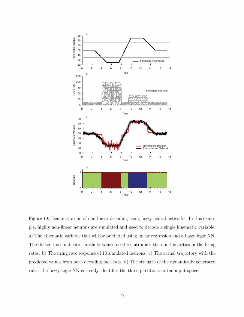
00
2 4 6 8 10 12 14 16 18
20
30
40
50
60
7080
00
2
1
4 6 8 10 12 14 16 18
0 2 4 6 8 10 12 14 16 180
50
100
150
200
250
0 2 4 6 8 10 12 14 16 1820
30
40
50
60
7080
Time
Time
Time
Time
Firin
g ra
te
Reverse Regression
Kine
mat
ic v
aria
ble
Stre
ngth
Kine
mat
ic V
aria
ble
a)
b)
d)
c)
Fuzzy Neural Network
Simulated neurons
Simulated kinematics
Figure 19: Demonstration of non-linear decoding using fuzzy neural networks. In this exam-
ple, highly non-linear neurons are simulated and used to decode a single kinematic variable.
a) The kinematic variable that will be predicted using linear regression and a fuzzy logic NN.
The dotted lines indicate threshold values used to introduce the non-linearities in the firing
rates. b) The firing rate response of 10 simulated neurons. c) The actual trajectory with the
predicted values from both decoding methods. d) The strength of the dynamically generated
rules; the fuzzy logic NN correctly identifies the three partitions in the input space.
77

100
110
120
130
140Hip Angle Prediction
Hip
Ang
le
0 5 10 15 20 25 300
0.2
0.4
0.6
0.8
1FNN Contribution of Rules (3 total)
Rul
e St
reng
th
Time (s) Rule strength indicators
A)
B)
Original Rev. Regression Fuzzy Neural Network
Figure 20: Example of a decoded hip angle during a center-out passive movement trial. A)
The hip angle plotted versus time and the estimates of the hip angle using reverse regression
decoding and fuzzy neural network decoding. B) The strength of the rules over time during
decoding using the fuzzy neural network. The sum of the strength of the rules equals 1 at
all times. It is clear that different rules are utilized for various states of the limb kinematics.
78

Although fuzzy neural networks are widely utilized by the engineering community to
implement non-linear controllers, alternative algorithms modeling non-linear behavior have
been proposed which are rooted in a more statistical reference frame. Spline regression
models provide a similar methodology to partition the input space and apply local linear
models for decoding. The next section will present decoding results using splines in an
extension of the reverse regression method.
4.2 SPLINE REVERSE REGRESSION
Instead of using fuzzy neural networks, one can extend the reverse regression models to allow
for non-linear effects of the firing rates on the kinematic variable. As described in section
2.2.2, we modeled each kinematic variable Ak as a function of the primary afferent firing
rates FR,
Ak = βk0 +∑i∈Sk
si(FRi) (4.7)
where s(.) indicates a spline and Sk the set of neurons used in the analysis.
Using the same data-set as the previous example, we plotted the estimates of hip-angle
using reverse regression and spline based reverse regression in figure 21. For this example
we used splines with 4 non-parametric degrees of freedom for all regression variables. As
expected, the spline based regression outperforms the reverse regression significantly.
Using splines, the input variable space is also sectioned and locally fitted. For each
regression variable, a linear or quadratic function is fitted for each of the sections marked
by the knots. Therefore, the number and location of the knots influence the variability of
the fitted model. As with fuzzy neural networks, model selection is the main difficulty when
using spline bases for the reverse regression method. Especially with the large number of
regression variables (the firing rates), there are an infinite number of feasible models. In
order to simplify the model selection, we can try to estimate the number and locations of the
knots for each regression variable separately and use the resulting knots for the kinematic
79

0 5 10 15 20 25 30100
110
120
130
140Hip Angle Prediction
Angl
e
Time (s)
Original Rev. Regression Spline Rev. Regression
Figure 21: Decoding center-out movement using spline reverse regression. Limb kinematic
predictions are shown for reverse regression and reverse regression using smoothing splines
with 4 degrees of freedom.
model described in equation 4.7. We can then proceed to eliminate knots from the new
model to minimize the degrees of freedom if necessary. Thus, in order to find an accurate
model for kinematic variable Ak, we first try to model this variable directly using each of
the recorded afferent firing rates individually.
We define the set of models Ak = βk0 + si(FRi), where we vary the number of knots
and/or their location. For example, we can start by performing a model selection on the
models with 1, 2 or 3 knots at equidistance. Model selection is used to determine the most
appropriate knot locations for that particular spline. Once this is done for all neurons, we
use the resulting knot locations as an initial guess for the splines in equation 4.7. We can
continue our model selection by randomly removing knots to minimize the degrees of freedom
in our kinematic model.
In summary, fuzzy logic neural networks are capable of describing a non-linear transfer
function in terms of a weighted average of linear functions. The methodology is relatively
easy to interpret which might be one of the reasons that the technique still is popular
amongst engineers for non-linear modeling. However, using non-parametric splines for non-
80

linear multivariate modeling can result in similar or better estimates and is well regarded
with the statistical community. Although the primary focus of this chapter has been on the
fuzzy neural networks as a result of the collaboration with Dr. Silvestro Micera, at the ARTS
laboratory of the Scuola Superiore Sant’Anna in Italy, it seems that regression splines should
be considered as the more viable option for improving the accuracy of decoded trajectories
in a ‘real-time’ neuroprostheses. Implementation of such methods in Labview and or Matlab
are currently being pursuit in the lab and will be used during subsequent experiments.
81

5.0 CLOSED LOOP CONTROL OF FUNCTIONAL ELECTRICAL
STIMULATION
A functioning demonstration of closed loop control of limb state using primary afferent
firing rates as the feedback loop for the controller is presented in this chapter. It will address
and discuss the hypothesis described in the 4th specific aim of this thesis. It combines
the techniques described in the previous chapters and provides a stepping stone for further
development towards continuous, stable and reliable feedback control of FES.
5.1 INTRODUCTION
Functional electrical stimulation (FES) has long been recognized as a viable way to restore
function in the extremities of paraplegic patients. Recognizing that the muscle is an efficient
actuator for limb movement, it is not surprising that many studies have focussed on the
implementation of FES for limb kinetic restoration. To date, multiple devices have been
developed and are commercially used such as, the bionic glove [81], the WalkAid [28, 107]
and the NESS Handmaster [42].
The Walk-aid is the only application within these examples that can be regarded as a
closed loop FES-system because stimulation is based on the angle of the shank of the affected
leg. When the subject reaches the end of the stance phase, the stimulator turns on, lifting the
foot which enables the swing phase to be executed appropriately. Despite this success story,
feedback sensors have proven difficult to implement in prosthesis due to their unreliability,
fragility and practical difficulties.
82

Despite these difficulties, it is widely recognized that a FES system would benefit tremen-
dously from sensory feedback in terms of adaptability and functionality as long as the feed-
back system would be reliable [79, 67]. With closed loop control of FES, it is possible to
change the stimulation parameters dynamically and make them dependent on the feedback
from the sensors. If accurate predictions of limb state are available to the FES controller, it
will be able to compensate for muscle fatigue and possibly be able to adjust for unexpected
perturbations of the extremity, e.g. stumbling.
Although the single external sensor works well in the case of the WalkAid, this approach
might not work as well when detailed multivariate information is required as the feedback for
the neuroprosthesis [67, 53]. Implantable sensors have been suggested as a viable alternative
to external sensors. In 2004, Tan et al. described a method to use the antenna coils of
implantable stimulation units (BIONs) to infer limb state variables. They conclude that
using such sensors can potentially be combined with other sensing techniques to ultimately
provide sufficient accuracy for closed loop control of FES for patients with paralysis [112, 111].
Alternatively, one can record from the natural sensors of the nervous system and decode
the limb state based on their neural response. Muscle spindles as well as golgi tendon
organs and cutaneous afferents are known to be contributors to proprioception although it is
generally accepted that the muscle spindles are the main contributors to proprioception [35].
The firing rate response of these afferents can be correlated to global kinematic variables
such as endpoint position of the extremity of joint angles (see section 1.1.3 ).
With current technology, it is possible to record simultaneously from many of those
afferents and previous research has showed that by recording from these afferent neurons in
the Dorsal Root Ganglia (DRG), it is possible to predict the limb state accurately throughout
a movement [106, 122, 119, 120]. In these experiments, the hind limb of a cat was passively
manipulated throughout various movement patterns while kinematics and primary afferents
were recorded. After the experiment, the data was analyzed and limb kinematics were
predicted using the recorded firing rates of the primary afferents. For neural prosthesis, a
realtime version has to be implemented that is capable of estimating the limb state in real
time.
83

There are various ways to implement the interface for electrical stimulation. Surface
stimulation and intra-musclular stimulation are the most direct method of activating the
muscles. Alternative methods have been proposed over the years such as selective stimulation
using a multi-site nerve cuff [62] and intra-spinal micro-stimulation [5, 41]. These methods
have the advantage that they require lower stimulation currents and have lower stimulation
artifacts as a result. In addition, these methods target multiple muscles using a single
interface which makes it attractive for clinical use. ISMS also claims to potentially activate
synergies of muscles which may be beneficial to the correct recruitment of muscle tissue [60].
In this work however, we used intramuscular stimulation as it is the easiest to implement
and the most reliable way to stimulate different muscles in an experimental setup.
The following sections investigate the feasibility of using primary afferent signals in a
‘real-time’ closed loop controller for FES. The work described in this chapter leading to-
wards the complete closed loop controller includes discussions about various aspects of this
engineering problem; 1) The real-time decoding algorithm will be discussed, 2) a method
for removing the stimulation artifacts and its implications on the decoded signal will be dis-
cussed and 3) a state-machine based stimulation controller is proposed as an initial approach
towards a closed loop FES controller.
5.2 METHODS
5.2.1 Surgical procedures
All procedures were approved by the Institutional Animal Care and Use Committee of the
University of Pittsburgh. Four animals were used in these procedures. Anesthesia was ini-
tiated using Isoflurane (1-2%) and switched to Alpha Chloralose for the duration of the
trials. Temperature, end tidal CO2, heart rate, blood pressure and oxygen saturation were
monitored continuously during the experiments and maintained within normal ranges. In-
travenous catheters were placed in the forelimbs to deliver fluids and administer drugs. A
laminectomy was performed on the left side and penetrating micro-electrode arrays (1.5mm
84

length, Blackrock Microsystems LLC, USA) were inserted in the L7 (50 electrodes in 10x5
grid) and L6 (40 electrodes in 10x4 grid) dorsal root ganglia. A combination of patch and
intramuscular stimulating electrodes were placed in various muscles spanning hip, knee and
ankle joints. Suitable locations for electrode placement were found by stimulating the site
with a mono-polar probe. At the conclusion of the experiments, the animals were euthanized
with KCL (120 mg kg−1).
5.2.2 Experiment setup
A custom frame was designed to support the cats torso, spine and pelvis while allowing the
hind limb to move freely through its full range of motion. A stereotaxic frame and vertebrae
clamp were used to support the head and torso, and bone screws were place bilaterally in
the iliac crests to tether the pelvis with stainless steel wire (see figure 22).
Neural data was sampled at 25kHz using an RZ-2 real time signal processing system
(Tucker Davis Technologies, USA). The neural data was filtered using a bandpass filter with
cutoff frequencies of 300 and 3000 Hz. Neural activity was defined as an event where the raw
recorded signal crossed a manually set threshold. This threshold was set manually for each
channel depending on the signal to noise ratio of the particular electrode. A snippet of 1ms
was recorded each time the signal crossed the threshold and the neural sources on a single
channel were discriminated using a k-means clustering algorithm which was implemented to
function on the recording hardware (RZ-2). Events (spikes) were binned for each independent
source in 50ms windows within the RZ-2 device and subsequently streamed over the ethernet
using the UDP protocol to the ‘real-time’ stimulation controller.
Kinematic data was captured using a high speed motion capture system (Impulse system,
PhaseSpace Motion Capture, USA). Joint angles for hip, knee and ankle were computed in
realtime using custom developed software and were streamed over the ethernet to the ‘real-
time’ stimulation controller using the UDP protocol. A haptic device (Phantom Premium
1.5HF, Sensable Technologies Inc, USA) was used to create an artificial floor and estimate
ground reaction forces during the FES trials. In addition, a slight viscous force field was
simulated to dampen the effect of stimulation and reduce unwanted oscillations.
85

TDT RZ-2Neural Data Acquisition System
Kinematic Markers
Stereotaxic head frame not shown
Electrodes
L6 & L7 dorsal root ganglia
CWE FNS1616 Channel Stimulator
Force Field
Figure 22: The animal was positioned in a custom designed frame to support the torso and
pelvis, enabling unrestrained movement of the left hind limb. Active markers were placed to
track the hind limb kinematics and a 90-channel micro electrode array was inserted in the
L6/L7 DRG to record neural activity. Intra-muscular electrodes were place in various hind
limb muscle to evoke movement and a phantom robot was attached to the foot to generate
an artificial floor by means of a force field (not shown).
86

Binned spike counts and joint angles were retrieved by the stimulation controller PC run-
ning custom analysis software developed in Labview (National Instruments, Austin, USA).
Binned spike counts were smoothed by convolving a triangular window (150ms) were paired
with the recorded kinematics. The joint data-structure was used to train and decode the
kinematic models. Both neural and kinematic data were processed in 50ms windows to
facilitate the software to compute the kinematic predictions. This conforms with low-pass
filtering methods used in previous experiments using reverse regression methods [122, 106].
5.2.3 Realtime encoding of firing rate models
Offline decoding limb kinematics from a population of primary afferents in the DRG has
been demonstrated previously using various decoding techniques such as reverse regression
and state-space modeling [106, 119, 120]. Although the state-space modeling algorithms
were found to be clearly superior to the previously used reverse regression techniques, we
implemented the latter because of implementation considerations (see chapter 4 for additional
information). For these experiments, we did not use any non-parametric splines as the
development package did not natively support this type of regression algorithm.
For this work, let X = (Xk, k = 1, . . . , K) be the vector of K kinematic variables we
want to decode, based on the firing rates FR = (FRi, i = 1, . . . , I) of I neurons. In this
work we considered two reference frames to express limb state (X); a joint-based frame with
state vector (Ak, k = 1, 2, 3) that represents intersegmental angles for the hip, knee, and
ankle joints, and a endpoint force frame with state vector (X,Z) that represents the vertical
and forward force generated at the endpoint of the extremity. A subscript t added to any
variable means that we consider the value of that variable at time t. The firing rates FR
were obtained by smoothing the incoming binned spike counts using a triangular window
spanning 150ms. Using reverse regression we can predict the joint angles and endpoint forces
by modeling these variables as a linear function of the observed firing rates, such that
Xk = βk0 +∑i∈Sk
βkiFRi + εk, (5.1)
87

where Sk indexes the set of neurons which were classified in realtime by the clustering
algorithm, and εk are uncorrelated random errors. The predictions are obtained by evaluating
the model at the observed firing rates.
5.2.4 Removing stimulation artifact
Stimulation of the muscles results in significant artifacts in the recorded neural data and can
potentially give rise to erroneous estimates of neural firing rates. Previous studies have used
input blanking to remove stimulation artifacts during recording, shielded the stimulation
sites to minimize artifacts [131] or used the fact that a stimulus artifact appears on all
channels simultaneously to eliminate these events in an offline analysis [123].
In order to estimate the effect of stimulation artifact on the recorded neural data and the
ability to record meaningful afferent responses, we simulated the amount of time stimulation
artifacts would mask the input channels as a function of the average stimulation frequency
and the number of independent channels of stimulation. Figure 23 shows the percentage of
time available for uncontaminated recording as a function of these variables. We can see
that the number of independent channels of stimulation significantly degrades the possibility
to record afferents. The circumvent this problem, we programmed the stimulation controller
such that all channels were synchronized during stimulation. The stimulation frequency was
set to 30Hz and the intensity of the stimulation was solely determined by the amplitude of
the stimulation pulses. At 30 Hz stimulation, muscles in general display tonic contractions.
By using synchronous stimulation of the electrodes, we can eliminate the effects of multiple
electrodes and, given a blanking window of 1ms, still have approximately 95% of the time
for neural decoding.
One problem with blanking the input channels during stimulation is that this introduced
discontinuities of the values on the input channels. As neural data are usually smoothed
before processing, this introduces unwanted oscillations following blanking. In the worst
case scenario, this could result in an unwanted spike event when the oscillations exceed the
channel threshold. In addition, blanking the inputs removes all data during that period and
makes offline analysis and verification of the method impossible.
88

10 20 30 40 50
0.5
0.6
0.7
0.8
0.9
1.0
Average Stimulation Frequency (Hz)
Dec
odin
g tim
e / t
otal
tim
e
● 1 Electrode3 Electrodes6 Electrodes12 Electrodes
Stimulation artifact duration: 1ms
● ● ● ● ● ● ● ● ● ●
Figure 23: Effects of blanking stimulus artifacts on the available time to record neural data.
As the average stimulation frequency increases or multiple electrodes are active in a non-
synchronous way, the remaining time for decoding the firing rates decreases. This plot was
generated using multiple simulations of multichannel stimulation. The decoding time was
defined as the time where no stimulation was occurring.
89

Detection window (DW)Rejection window (RW)
Stimulation
Activity
Blanked activity
If DW > TH ignore(RW )
TH = threshold sum of spikes
Figure 24: This simulated schematic describes the stimulation artifact removal algorithm as
implemented on the RZ2 DSPs. Spike activity from all channels is represented on a single
time-axis. The number of spikes recorded during the detection window (DW) are summed
and if this number exceeds a threshold (TH = 0.9*number of channels), all recorded spikes
in the rejection window (RW) are ignored. The size of RW can be equal or bigger than the
size of the DW.
Using a state of the art neural data acquisition system, we were able to implement a
hardware based version of the synchronous event detection algorithm. Figure 24 shows the
implemented method. We defined a small time window (DW = 1ms) and summed all
recorded events within at each time-point. In case more than 90% of the channels recorded
a spike during that interval, all spikes in the rejection window RW were excluded from
the calculation of the instantaneous firing rates of the units. The RW could be set to
an arbitrary length and could be used to exclude afferent responses generated by direct
stimulation of the afferent fibers. The instantaneous firing rate was subsequently calculated
per unit on the neural data acquisition system and streamed over the ethernet using the UDP
protocol. Using this artifact rejection method, all signals including stimulation artifacts will
be recorded for offline analysis while they will be omitted during the realtime control of FES.
90

5.3 RESULTS
Data from multiple closed loop FES experiments are presented in this section. As previous
chapters discussed the ability to decode limb kinematics from primary afferent firing rates in
detail, no example will be given in this chapter. Analysis of realtime encoding and decoding
of limb kinematics will be presented in section 5.3.1. Section 5.3.2 will present data on the
ability to decode during functional electrical stimulation and finally, section 5.3.3 will present
an example of closed loop FES.
5.3.1 Realtime decoding of primary afferents
An example of real-time decoding using reverse regression is presented in figure 25. Here,
the hindlimb was passively manipulated through a series of center-out movement tasks.
At t = 0s, the kinematics and observed instantaneous firing rates were used to update
models for the kinematic parameters (joint angles). At t = 60s, the estimated models were
used in combination with the observed firing rates to predict the kinematics. The results
in figure 25 were produced during the trial and not manipulated afterwards. The typical
noisy characteristic of reverse regression and the incorrect predictions during high velocity
movement (overshoot) can easily be seen although the overall predicted values for hip, knee
and ankle angle seem accurate.
Figure 26 shows the progression of the coefficients during the ‘realtime’ encoding process
during a random walk passive movement test. The bottom panel shows the joint angles
for hip, knee and ankle during the encoding process and the top panel shows a heat-map
representing the influence of each neuron in the model of the accompanying kinematic vari-
able. The influence was calculated by multiplying the value of the coefficient by the the
maximum firing rate of that neuron over the course of the encoding process. Subsequently
all resulting values were normalized to fall within a range of [-1,1]. The encoding algorithm
was implemented in Labview and developed such that the models were updated as fast as
possible during the trial which resulted in an update rate from 200ms to 3 seconds as the
encoding trial progressed.
91

50
60
70
80
80
100
120
140
0 20 40 60 80 100 12040
60
80
100
120
Real Time Estimation of Joint Angles during Center Out movement
Hip
Ang
leKn
ee A
ngle
Ankl
e An
gle
Time (s)
TrainingEstimating
Figure 25: Realtime encoding and decoding of the firing rates of primary afferents during a
passive center-out movement trial. During the first minute, the kinematic and the observed
firing rates are used to encode the kinematic models, during the second minute the observed
firing rates are used to predict limb kinematics.
92
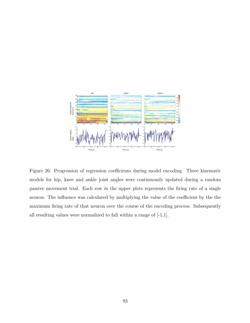
0 20 40 60 80
5
10
15
20
25
30
35
40
0 20 40 60 8066
68
70
72
74
76
78
0 20 40 60 80
0 20 40 60 8070
80
90
100
110
120
130
0 20 40 60 80
0 20 40 60 8040
50
60
70
80
90
100
-1
-0.8
-0.6
-0.4
-0.2
0
0.2
0.4
0.6
0.8
1
Time (s) Time (s) Time (s)
HIP KNEE ANKLE
COEF
FICI
ENTS
Neur
on n
r. JO
INT
ANG
LE(d
eg)
Figure 26: Progression of regression coefficients during model encoding. Three kinematic
models for hip, knee and ankle joint angles were continuously updated during a random
passive movement trial. Each row in the upper plots represents the firing rate of a single
neuron. The influence was calculated by multiplying the value of the coefficient by the the
maximum firing rate of that neuron over the course of the encoding process. Subsequently
all resulting values were normalized to fall within a range of [-1,1].
93

The neurons corresponding to each row are matched across the different models. This
implies that some of the same neurons heavily influence the predictions of multiple models.
In addition, we can see that a relatively large group of neurons have equal contributions for
the hip model whereas for knee and ankle, a limited set of neurons convey all information
about the kinematic variable.
5.3.2 Decoding during stimulation
Decoding during FES requires the controller to dismiss stimulation artifact. Figure 27 shows
that the observed firing rates of primary afferents continue to provide information about
limb state during stimulation. Here, the hind limb was manipulated through a series of
flexion and extension movements using a robotic manipulator. During the second set of
movements, electrical stimulation was applied to generate stimulation artifact at a rate of
30 Hz. The location and amplitude of the stimulation was chosen such that no significant
muscle force was generated during these trials. It can be seen that the example neurons carry
information about ankle position under both scenarios. This demonstrates that information
can be extracted from the primary afferent population in the presence of FES.
To demonstrate that the primary afferent neurons continue to generate graded responses
to the desired variables, we used FES to generate ground reaction forces in a semi-isometric
preparation. Here, the foot was strapped to a stationary force transducer. Limb extensors
were stimulated at 30 Hz over a prolonged period of time to induce fatigue. The stimulation
was alternated on/off manually to generate an alternating pattern of ground reaction forces.
Figure 28 shows the neural response as well as the stimulation times. Overlaid is a prediction
of the ground reaction forces based on the primary firing rates recorded in the DRG. The
ability to track the forces during fatigue demonstrates that the decoded forces are not merely
tracking the periods of stimulation.
94

Ankle Position
Unit 1Fi
ring
Rat
e (s
p/s)
60
0
Unit 2
Time (s)0
110
400 Time (s) 500
Stimulation
Figure 27: Primary afferent firing rates recorded during passive flexion and extension of
the hind-limb with and without stimulation. It can be seen that the firing rate response of
both units is maintained during stimulation of the leg. In this scenario the amplitude of the
stimulation created significant artifacts during recording but did not produce any significant
activation of a muscle.
0 10 20 30 40 50 60 70 80 90-20
-10
0
10
Forc
e (N
)
Time (s)
Ground reaction force Force prediction
Figure 28: Decoding ground reaction forces during functional electrical stimulation. The
stimulation was manually triggered and forces were recorded with the foot fixed to a sta-
tionary load cell. Fatigue of the muscle is accurately predicted using primary afferent firing
rates during stimulation.
95
5.3.3 Closed loop control of FES
Labview was used to implement a ‘real-time’ closed loop FES controller which was capable of
switching stimulations parameters using a state machine triggered by the endpoint kinemat-
ics of the hindlimb (actual or predicted). Figure 30 shows the front-end of this state machine
as well as some of the trajectories obtained using FES on multiple channels. This display is
similar to the display used to define the state-machine during the actual experiments.
The hindlimb is represented by a stick-figure with segments between the Iliac Crest
and the Hip, Hip-Knee, Knee-Ankle and Ankle-Foot. The state machine can be configured
by ‘drawing’ boxes in the workspace to indicate the regions in which the controller should
increment the state of the stimulation paradigm and accompanying stimulation parameters.
In this case, we defined 4 states. The transition between the states was initiated when
the endpoint of the hind limb entered a switch point section and remained there for a
predetermined amount of time. Transitions between states could be set to instantaneously
or could be changed gradually by fading in/out of the stimulation amplitudes. All channels
were set to stimulate at 30 Hz in synchrony to minimize the stimulation artifacts.
Prior to the trial, we selected a subset of stimulation channels per state such that the
resulting limb movement was directed towards the next stimulation switch location. We could
do so by selecting individual channels and amplitudes per state. Minimum and maximum
stimulation period were enforced such that the trial was aborted when the next box was not
reached.
Figure 30 also shows some recorded trajectories during a closed loop trial. In this par-
ticular case, we switched the stimulation states based on the kinematics recorded with the
camera setup. Other trials using the predicted kinematics from the neural data showed
similar results, albeit a little less accurately.
96

200
260 A)
B)
C)
D)
Hip
-to-to
e di
stan
ce (m
m)
Stim
ulat
ion
0
250
Uni
t firi
ng ra
te (s
p/s)
0 350
120
Time (s)
Figure 29: Limb movement and afferent responses during a closed loop stepping trial in which
movement was created by FES using 9 channels and 4 different states in the state-machine.
A) The kinematic variable indicting the distance between the hip and toe marker. B) The
stimulation pulses on 9 channels; the red lines indicate the 4 different stimulation patterns.
C) and D) show the response of two primary afferent neurons, both neurons correlate with
the kinematics independently of the stimulation.
97

Subsequently, we imposed perturbations to the leg by obstructing its movement during
stimulation (not shown). This resulted in prolonged period of stimulation of the same pattern
as the leg was not able to reach the following state switch point. Although the estimates
of limb state were sufficient to drive the state-machine during these closed loop trials, the
accuracy of the decoded trajectories has room for improvement. New decoding methods,
such as those proposed in the previous chapters, should provide the required improvements
and will be implemented in future experiments.
Figure 29 shows the response of two primary afferent neurons during the closed loop
stimulation. In A), we plotted the distance between the hip marker and the toe marker
for a series of FES evoked steps. As the foot is placed forward (First red dotted line), we
can see some oscillations resulting from the simulated floor created by the haptic device.
Subsequently, the foot is pushed back, lifted up and moved forward before repeating the
sequence.
The second panel (B) shows the stimulation sequence on the 9 implanted stimulation
sites. We can see the four distinct patterns responsible for the different stages in the step-
cycle. Panels C) and D) show the response of two units which are correlated to the kinematic
variables. During these trials, all recorded unit activity was used to decode the kinematics;
that is, there was no selection of neurons used for decoding.
5.4 DISCUSSION
A closed loop neural prosthesis should be regarded as a complex system integrating different
challenges such as afferent recording, kinematic state decoding, actuating the muscles and the
accompanying control algorithms. The results presented in this chapter should be regarded
as an initial attempt to combine these challenges in order to understand the complexity of
the task. We showed that with the current technology, it is possible to develop a rudimentary
closed loop FES controller which is able to generate walking-like behavior in a closed loop
fashion.
98

00 50 100 150 200
50
100
150
200
250
t = 6.75:11.50s
Position (mm)
State switch locationsPosi
tion
(mm
)Predicted trajectoryActual trajectory
hip
knee
Figure 30: Example trajectories produced by closed loop FES. The solid thick black stick
figure represents the hind limb of the animal and the endpoint is used to trigger the state-
machine. The state switch location boxes can be positioned by the experimenter and indicate
the areas where the state-machine should switch stimulation parameters. The displayed
boxes are an approximate location in this particular trial. The black thin line represents the
actual limb endpoint kinematics over 4 cycles and the red dotted line represents the limb
endpoint prediction using the firing rates of the recorded primary afferent neurons.
99

Although reverse regression has been proven to provide good estimates of limb kinemat-
ics, recent work has shown that other decoding techniques can improve the estimates signif-
icantly. State-space decoding improves the resulting estimates by a factor of two. However,
this decoding technique is not fast enough to be implemented in real time. An alternative
is to use a fuzzy logic decoding algorithm. Rigosa et al. showed that this type of decoder
can also improve the estimates significantly in an offline situation [89]. Fuzzy logic decoding
sections the input variable space and defines a linear model for each subspace. Limb kine-
matics are inferred by a weighted average of the models where the weights are determined
by a measure of proximity of the inputs to each section. The previous chapter also intro-
duced spline regression as a viable extension to reverse regression. Challenges will include
the implementation of such decoders in a ‘real-time’ environment as currently developed in
Labview.
Alternatively, as the stimulation parameters are driven by a state-machine, it can be
suggested to use a classifier decoding method rather than a continuous representation of
limb angles. Such a method could predict the likelihood of the leg being in one of the
switching states. Such a method might result in more robust state switching but will loose
the ability to track the limb-state variables.
Artifact rejection is an integral part of a closed loop controller using functional electrical
stimulation as the muscle activator. We showed that when the stimulation paradigm is
tuned to minimize the stimulation artifact by aligning stimulation on different channels,
it is possible to remove the stimulation artifacts without losing the ability to decode limb
state variables from the primary afferent population. Although direct stimulation artifacts
are relatively easy to identify and reject based on amplitude and wave-shape, this is not
the case for artifact arising from direct stimulation of the afferent neurons as the recorded
signal will be indistinguishable from a neural response related to a change in limb state.
However, synchrony detection across a large number of channels might be able to separate
the different scenarios. This type of artifact could potentially be greatly reduced by changing
the stimulation paradigm.
100

A vast body of research has been published on the application of functional electrical
stimulation as a means of reanimating paralyzed extremities. Intra-spinal micro stimulation
(ISMS) has been suggested as an alternative to intra-muscular and surface stimulation during
the recent years [5, 41]. ISMS has the advantage that it uses very small stimulation artifacts
as compared to surface stimulation and can potentially activate synergies of muscles which
may be beneficial to the correct recruitment of muscle tissue [60]. Using the DRG or the
ventral roots as the location for stimulation has also been suggested as an alternative location
[5]. Our lab is currently investigating the feasibility of using these alternative locations for
stimulation.
The relationship between muscle length and joint or limb position is typically complex
and in many cases indeterminate [9], suggesting that other sources of feedback are required
to resolve ambiguities in spindle feedback related to joint position [26]. In addition, sensory
receptors as the muscle spindle are innervated by modulated motor neurons (γ) that change
the behavior of the sensors constantly. Spinal cord injuries change this descending neural
track and therefore alter the afferent coding scheme. The impact of this change on the
ability to decode accurately from the afferent population is unknown but highly relevant for
applications of FES while spinal cord patients are part of the target population.
In summary, a closed loop neural prosthesis comprises a complex system integrating dif-
ferent challenges such as afferent recording, kinematic state decoding, actuating the muscles
and the accompanying control algorithms. The results presented in this chapter should be
regarded as an initial attempt to combine these challenges in order to understand the com-
plexity of the task. They showed that with the current technology, it is possible to develop
a rudimentary closed loop FES controller which is able to generate walking like behavior in
a closed loop fashion.
Advancements in the neural engineering field are largely reliant of improvements of the
stability and reliability of the neural interfaces used in these applications. Continuing efforts
to improve FES control, afferent decoding and interface technology should be pursued to
enable the use of closed loop FES neuroprostheses in the future.
101

6.0 GENERAL DISCUSSION
In this final chapter of my thesis, I will elaborate on the results presented in this work as
well as provide my view on the necessary research to be conducted extending the presented
work. Section 6.1 will summarize and discuss the findings in this work and section 6.2 will
discuss its significance in the bioengineering field and suggest directions for future work.
6.1 SUMMARY
It is believed that the nervous system represents the kinematic state of extremities in various
ways throughout the nervous system [38, 11, 12]. An interface with the nervous system to
extract this sensory information would significantly aid the development of advanced neu-
roprostheses using FES to animate paralyzed extremities. By means of sensory integration,
the CNS is thought to be able to reduce the highly redundant input space into a representa-
tion of limb state that is more useful to process. The location of the interface can therefore
influence the types of signals we are able to extract. The work presented in this document
has focussed solely on the sensory nervous system at the level of the DRG; the firing rates
of the individual sensory neurons.
The foundation for the work presented in this thesis originates with the work of Stein
and Weber who presented methods for decoding limb kinematics from the firing rates of
populations of primary afferent neurons in [105, 122]. In chapter 2, we provided a more
generalized and principled method for decoding limb kinematics from the firing rates of
primary afferent neurons. We showed that by modeling the firing rate of the primary afferents
102

instead of modeling the kinematic variables, the decoder could take into account that the
firing rate of an afferent neurons could be non-linearly related to multiple kinematic variable.
Subsequently, in chapter 3, we extended these methods to be able to incorporate velocity
components of the firing rate. In addition, we showed how state-space modeling can be
used to predict multiple correlated kinematic variables in a principled way. The resulting
estimates of limb state were on average twice as accurate as previously suggested methods
(reverse regression). Although the results of state-space modeling were promising, it required
significant computing power to execute and was therefore not ready for implementation in
a ‘real-time’ environment at this time.
Chapter 4 discussed some alternative methods for decoding limb kinematics that would
be fast enough to implement in ‘real-time’. Fuzzy neural networks have been proposed to
find a set of input-output relations describing a non-linear process [108]. We showed that
an adapted version of the TSK fuzzy logic decoder can be used to decode limb kinematics
and improve decoding accuracy over reverse regression. Alternatively we found that spline
regression shows equal improvements over reverse regression and is more principled and easier
to implement than fuzzy neural networks. Although both methods improve upon reverse
regression, they are not as principled as state-space modeling because velocity components
and the coupling between kinematic variables are not taken into account.
Finally, in chapter 5, various aspects and challenges of a closed loop FES neuroprosthesis
are presented. A ‘real-time’ controller was implemented and it was shown that the firing
rates of primary afferents could be recorded, sorted and used for decoding limb kinematics
in such a setup. Stimulation artifacts were removed in hardware using a sliding window and
a synchronous detection algorithm. The FES controller was updated using a state-machine
based on the predicted limb kinematics.
In summary, the work in this thesis provides methods for decoding primary afferent
neurons and sets a foundation for further development of closed loop FES control of paralyzed
extremities. Although a complete closed loop neuroprosthesis for natural behavior seems far
away, the premise of this work argues that an interface at the dorsal root ganglia should be
considered as a viable option.
103

6.2 SIGNIFICANCE AND FUTURE WORK
Functional electrical stimulation has been regarded as highly potential for restoring func-
tionality in hemi/paraplegic patients. It has been proven to facilitate improved hand func-
tionality [81], standing capability [29, 30], improved walking capability [107] and is used in
many other applications. Using muscles to generate movement might be the most power
efficient way to displace extremities which facilitates assisted movement of extremities with
a relatively small power source. In addition, FES helps the body to maintain muscle mass,
rigidity, and in general be in a more healthy state.
However, FES applications suffer from multiple drawbacks that require additional atten-
tion before FES can be used reliably as a means to restore the functionality of an affected
extremity. One of the most important issues that need to be addressed is how to measure
the actual kinematic state of the limb while using the prosthesis to facilitate closed-loop
control of FES [44]. Exteriorly placed sensors such as gyroscopes and goniometers, force
sensors and stretch sensors have been proposed and tested in closed loop FES applications
[78, 28, 103]. Although these options are viable when limited information is needed, the use
of exterior placed sensors rapidly becomes difficult due to practicality issues when multiple
degrees of freedom are necessary. Therefore, the use of the body’s own sensory signals has
seen an increasing amount of attention and has been the focus of this dissertation.
Fundamental knowledge of the mechanisms and nature of proprioception is necessary to
understand the neural processes responsible for motor planning, control, and adaptation.
Despite a large body of literature that describes many details of primary afferent response
characteristics, and their projections to intra-spinal networks and ascending pathways to the
brain, relatively little is known about the actual neural coding and decoding processes that
support representations of limb state at any level of the sensory system. Thus, there are
several fundamental, yet unanswered questions about the nature of somatosensory feedback.
Which state variables are represented and which classes of afferent neurons contribute to the
neural representation of each state variable? Although this thesis has mostly focussed on
the practicality of using primary afferents for neuroprostheses, more knowledge about the
104

physiology, interactions and changes of primary afferent firing rates as a result of spinal cord
injury will likely be beneficial to the development of viable neuroprostheses.
This work has argued that afferent feedback is required to be able to compensate for
fatigue and account for unexpected perturbations as represented schematically in figure 5.
However, in the particular scenario where the person has impaired motor control but intact
sensory perception, one could argue against the need to decode the afferent signals for closed
loop control of FES. Although not represented in figure 5, direct connections exist between
sensory and motor areas in the higher regions of the CNS which might provide an adequate
feedback loop in this scenario. Therefore, when afferent pathways remain intact and the
patient only suffers from diminished motor control, it is possible that feedback loops in
higher regions of the CNS are sufficient to compensate the motor intent signal to the FES
controller.
It has been shown that a monkey can control a robot arm using cortical signals with
increasing accuracy and degrees of freedom [38, 117]. However, state feedback of the robotic
arm is purely visually in these experiments. An interesting extension of this work would
be to investigate whether proprioception will provide alternative/additive information which
could potentially result in better control of the neural prosthesis. This untested hypothesis
would be interesting to explore in an animal model as this could give us direct insight in the
flexibility of higher regions in the CNS to afferent information.
In order to address these questions, one could surgically sever the ventral roots innervat-
ing one of the upper extremities in a monkey while leaving the dorsal roots intact. Alterna-
tively, one could use botulinum toxin (BOTOX R©) to temporarily paralyze the muscles while
leaving the afferent response intact. Although both methods would also affect the gamma
motor drive to muscle spindles, it would provide a good model for the investigated scenario.
The affected extremity could then either be fitted with a custom exoskeletal robotic manip-
ulator or with surgically implanted FES electrodes (BOTOX R©inhibits Acetylcholine release
and it should therefore still be possible to use direct stimulation of the muscles using FES).
Results of reaching/drawing tasks could be compared to results obtained using only visual
feedback.
105

In the neural engineering community, there has been a steady search for the coordinate
frame in which the CNS encodes proprioception. In 2000, Bosco and Poppele presented
studies in which they claimed that secondary afferent neurons in the dorsal spinocerebellar
tract (DSCT) can signal foot position independently from the specific joint angles [12].
This could suggest that an abstraction of the primary afferent sensory space is performed
at relative low levels of the CNS. However, a closer look at their observations raises the
question whether the conclusions they present really reflect the observed behavior of the
DSCT neurons. For example, figure 8 in [12] is supposed to show that a neuron is invariant
to endpoint position while having different behavior in joint angle space when its response
is compared in a restraint and passive movement task. They argue that the data during the
passive trial can best be described by a linear function whereas the data in the constraint
trial is best described by a quadratic. However, this is most likely caused by the fact that
the range of motion of the hip angle is drastically smaller in the passive trial than in the
constraint trial. In my opinion, it is very likely that if the researchers would have ‘forced’
to record data over the same movement range, it would look exactly similar. As it might
be hypothesized that the neuron used for in the paper is a better than average example,
it seems that there is insufficient evidence from either statistical point or visually to infer
any underlying mechanisms in my opinion. They correctly conclude that an alternative
explanation is that the DSCT cells respond to additional unmeasured input variables such
as forces acting on the joint as a result of their setup [12].
In general, we should be very careful about statements explaining how the CNS interprets
the afferent firing rates and kinematic variables. Statements about the CNS representing
limb state only in endpoint coordinates can easily be rejected as this kinematic representation
is our ability to sense and we obviously experience more than pure endpoint positions of our
extremities. This does not mean that a reduced kinematic representation cannot be found
somewhere in our CNS but does prove that the CNS does not directly integrate all afferent
inputs to form a very reduced variable space before processing it in higher regions of the
CNS.
106

Over the last couple of years, we advanced from offline reverse regression methods to
state space modeling and ‘real-time’ FES applications. Specifically looking at the ‘real-time’
application, I think that we could have focussed more directly on a decoding method based
on state classification rather than continuous decoding. The advantage of classifiers is that it
directly address the events you are interested in. Especially in gait, this might be a more solid
and robust solution to switch between the different stimulation states. However, a continuous
prediction of limb kinematics might be advantageous when more detailed information is
required. For example, if we want to detect perturbations and unexpected events. The
reason we decided to start with the continuous predictions is that it relates to previous
published work for decoding primary afferent firing rates in an offline setup.
An unmentioned, but interesting, topic concerning FES neuroprosthesis is the location
of the stimulation. We used intra-musclular electrodes for stimulation during the closed
loop experiments because of their practicality and easy of implementation. However, the
large currents necessary for muscle animation produced significant stimulation artifacts.
In addition, this type of stimulation is prone to activating the sensory receptors directly,
resulting in a distorted representation of limb kinematics directly following a stimulation
pulse. Intra-spinal microstimulation has been suggested as an alternative strategy which
lacks the drawback previously mentioned but has shown mixed results as well [109, 60].
Using the DRG or the ventral roots as the location for stimulation has previously been
suggested as an alternative location [5]. Unpublished experiments in our lab show that
micro-stimulation in these areas show potential as they can selectively activate different
muscle groups. Additional research will have to investigate the feasibility in more detail.
Finally, as mentioned in previous chapters, the physical interface with the nervous system
is a crucial point of interest for neuroprostheses and its stability and reliability needs to be
addressed before any decoding efforts can successfully be used to provide limb state feedback
for controlling neural prostheses.
107

6.3 FINAL THOUGHTS
In pursuit of functional applications for neuroprostheses, one should realize that state of
the art hardware and software will continue to be one of the drivers behind their success or
failure. The experimental setup required for experiments towards these goals tend to grow
increasingly complex and the quantity of processed data require serious investments towards
analysis strategies. As this trend continues, it will be important to develop standardized
protocols for data interaction, manipulation and storage in order to maintain an efficient
research facility.
In addition, as the technology advances and the reality of bi-directional brain computer
interfaces inches closer, collaborations between the fields of Bioengineering, Robotics, Neu-
roscience, Computer science and Statistics will be more important with every step. One
of the biggest challenges will be to combine the knowledge in these fields and to rely on
each-others expertise.
108

BIBLIOGRAPHY
[1] E D Adrian. The impulses produced by sensory nerve endings: Part i. J Physiol,61(1):49–72, Mar 1926.
[2] E D Adrian and Y Zotterman. The impulses produced by sensory nerve-endings: Partii. the response of a single end-organ. J Physiol, 61(2):151–71, Apr 1926.
[3] E Alnaes, J K Jansen, and T Rudjord. Fusimotor activity in the spinal cat. ActaPhysiol Scand, 63:197–212, 1965 Mar.
[4] Y Aoyagi, R B Stein, A Branner, K G Pearson, and R A Normann. Capabilities ofa penetrating microelectrode array for recording single units in dorsal root ganglia ofthe cat. J Neurosci Methods, 128(1-2):9–20, Sep 2003.
[5] Yoichiro Aoyagi, Vivian K Mushahwar, Richard B Stein, and Arthur Prochazka. Move-ments elicited by electrical stimulation of muscles, nerves, intermediate spinal cord, andspinal roots in anesthetized and decerebrate cats. IEEE Trans Neural Syst Rehabil Eng,12(1):1–11, 2004.
[6] R S Arutiunian. Changes in the sensitivity of the muscle spindles of fast and slow-contracting muscle fibers following chronic de-efferentation. Neirofiziologiia, 13(2):204–209, 1981.
[7] D J Bennett, S J De Serres, and R B Stein. Regulation of soleus muscle spindlesensitivity in decerebrate and spinal cats during postural and locomotor activities. JPhysiol, 495 ( Pt 3):835–850, 1996 Sep 15.
[8] Rajmohan Bhandari, Sandeep Negi, and Florian Solzbacher. Wafer-scale fabricationof penetrating neural microelectrode arrays. Biomed Microdevices, 12(5):797–807, Oct2010.
[9] J Biggs and K Horch. Biomechanical model predicts directional tuning of spindlesin finger muscles facilitates precision pinch and power grasp. Somatosens Mot Res,16(3):251–262, 1999.
109

[10] Jaimie F Borisoff, Lowell T McPhail, James T W Saunders, Gary E Birch, and Matt SRamer. Detection and classification of sensory information from acute spinal cordrecordings. IEEE Trans Biomed Eng, 53(8):1715–1719, 2006.
[11] G Bosco and R E Poppele. Reference frames for spinal proprioception: kinematicsbased or kinetics based? J Neurophysiol, 83(5):2946–2955, 2000.
[12] G Bosco, R E Poppele, and J Eian. Reference frames for spinal proprioception: limbendpoint based or joint-level based? J Neurophysiol, 83(5):2931–2945, 2000.
[13] G Bosco, A Rankin, and R Poppele. Representation of passive hindlimb postures incat spinocerebellar activity. J Neurophysiol, 76(2):715–26, 1996.
[14] L J G Bouyer and S Rossignol. Contribution of cutaneous inputs from the hindpaw tothe control of locomotion. i. intact cats. J Neurophysiol, 90(6):3625–3639, 2003.
[15] L J G Bouyer and S Rossignol. Contribution of cutaneous inputs from the hindpaw tothe control of locomotion. ii. spinal cats. J Neurophysiol, 90(6):3640–3653, 2003.
[16] A Branner and R A Normann. A multielectrode array for intrafascicular recording andstimulation in sciatic nerve of cats. Brain Res Bull, 51(4):293–306, Mar 2000.
[17] A Branner, R B Stein, E Fernandez, Y Aoyagi, and R A Normann. Long-term stimula-tion and recording with a penetrating microelectrode array in cat sciatic nerve. IEEETrans Biomed Eng, 51(1):146–157, Jan 2004.
[18] A E Brockwell, A L Rojas, and R E Kass. Recursive bayesian decoding of motorcortical signals by particle filtering. J Neurophysiol, 91(4):1899–907, 2004.
[19] AE Brockwell, RE Kass, and AB Schwartz. Statistical signal processing and the motorcortex. In Proceedings of the IEEE, volume 95, pages 881–898, 2007.
[20] E N Brown, L M Frank, D Tang, M C Quirk, and M A Wilson. A statistical paradigmfor neural spike train decoding applied to position prediction from ensemble firingpatterns of rat hippocampal place cells. J Neurosci, 18(18):7411–7425, Sep 1998.
[21] E N Brown, L M Frank, D Tang, M C Quirk, and M A Wilson. A statistical paradigmfor neural spike train decoding applied to position prediction from ensemble firingpatterns of rat hippocampal place cells. J Neurosci, 18(18):7411–25, Sep 1998.
[22] Jane H Burridge, Morten Haugland, Birgit Larsen, Ruth M Pickering, Niels Svaneborg,Helle K Iversen, P Brøgger Christensen, Jens Haase, Jannick Brennum, and ThomasSinkjaer. Phase ii trial to evaluate the actigait implanted drop-foot stimulator inestablished hemiplegia. J Rehabil Med, 39(3):212–8, Apr 2007.
[23] Ettore Cavallaro, Silvestro Micera, Paolo Dario, Winnie Jensen, and Thomas Sinkjaer.On the intersubject generalization ability in extracting kinematic information from
110

afferent nervous signals. IEEE transactions on bio-medical engineering, 50(9):1063–73,Sep 2003.
[24] Cynthia A Chestek, Vikash Gilja, Paul Nuyujukian, Ryan J Kier, Florian Solzbacher,Stephen I Ryu, Reid R Harrison, and Krishna V Shenoy. Hermesc: low-power wirelessneural recording system for freely moving primates. IEEE Trans Neural Syst RehabilEng, 17(4):330–8, Aug 2009.
[25] D F Collins and A Prochazka. Movement illusions evoked by ensemble cutaneous inputfrom the dorsum of the human hand. J Physiol, 496 ( Pt 3):857–71, Nov 1996.
[26] D F Collins, K M Refshauge, and S C Gandevia. Sensory integration in the perceptionof movements at the human metacarpophalangeal joint. J Physiol, 529 Pt 2:505–515,2000.
[27] X Cui, V A Lee, Y Raphael, J A Wiler, J F Hetke, D J Anderson, and D C Martin. Sur-face modification of neural recording electrodes with conducting polymer/biomoleculeblends. J Biomed Mater Res, 56(2):261–72, Aug 2001.
[28] R Dai, R B Stein, B J Andrews, K B James, and M Wieler. Application of tilt sensorsin functional electrical stimulation. IEEE Trans Rehabil Eng, 4(2):63–72, 1996.
[29] R Davis, T Houdayer, B Andrews, and A Barriskill. Paraplegia: prolonged stand-ing using closed-loop functional electrical stimulation and andrews ankle-foot orthosis.Artif Organs, 23(5):418–420, 1999.
[30] M J Dolan, B J Andrews, and P H Veltink. Switching curve controller for fes-assistedstanding up and sitting down. IEEE Trans Rehabil Eng, 6(2):167–171, 1998.
[31] John P. Donoghue. Bridging the brain to the world: A perspective on neural interfacesystems. Neuron, 60(3):511 – 521, 2008.
[32] D Durand, H Park, and B Wodlinger. Localization and control of activity in peripheralnerves. Engineering in Medicine and Biology Society, Jan 2008.
[33] B Edin. Cutaneous afferents provide information about knee joint movements in hu-mans. J Physiol, 531(Pt 1):289–297, 2001.
[34] James B Fallon and Vaughan G Macefield. Vibration sensitivity of human musclespindles and golgi tendon organs. Muscle Nerve, 36(1):21–9, Jul 2007.
[35] S C Gandevia, D I McCloskey, and D Burke. Kinaesthetic signals and muscle contrac-tion. Trends Neurosci, 15(2):62–5, Feb 1992.
[36] S. C. Gandevia, J. L. Smith, M. Crawford, U. Proske, and J. L. Taylor. Motor com-mands contribute to human position sense. Journal of Physiology, 571(3):703–710,2006.
111

[37] Simon C Gandevia, Kathyrn M Refshauge, and David F Collins. Proprioception:peripheral inputs and perceptual interactions. Adv Exp Med Biol, 508:61–68, 2002.
[38] A P Georgopoulos, A B Schwartz, and R E Kettner. Neuronal population coding ofmovement direction. Science, 233(4771):1416–9, 1986.
[39] E V Goodall, T M Lefurge, and K W Horch. Information contained in sensory nerverecordings made with intrafascicular electrodes. IEEE Trans Biomed Eng, 38(9):846–50, Sep 1991.
[40] G E Jr Goslow, R M Reinking, and D G Stuart. The cat step cycle: hind limb jointangles and muscle lengths during unrestrained locomotion. J Morphol, 141(1):1–41,1973.
[41] Lisa Guevremont, Jonathan A Norton, and Vivian K Mushahwar. Physiologically basedcontroller for generating overground locomotion using functional electrical stimulation.J Neurophysiol, 97(3):2499–2510, 2007.
[42] H. T. Handricks, M. J. LJzerman, J. R. deKroon, and G. Zilvold. Functional electricalstimulation by means of the ’ness handmaster orthosis’ in chronic stroke patients: Anexploratory study. Clinical Rehabilitation, 15(2):217–220, 2001.
[43] R.R Harrison, R.J Kier, C.A Chestek, V Gilja, P Nuyujukian, S Kim, L Rieth, D.JWarren, N.M Ledbetter, S.I Ryu, K.V Shenoy, G.A Clark, and F Solzbacher. A wire-less neural interface for chronic recording. Proceedings of the 2008 IEEE BiomedicalCircuits and Systems Conference, 2008.
[44] M Haugland and T Sinkjaer. Interfacing the body’s own sensing receptors into neuralprosthesis devices. Technol Health Care, 7(6):393–399, 1999.
[45] M.K. Haugland and T. Sinkjaer. Cutaneous whole nerve recordings used for correctionof footdrop in hemiplegic man. Rehabilitation Engineering, IEEE Transactions on,3(4):307 –317, December 1995.
[46] J F Hetke, J L Lund, K Najafi, K D Wise, and D J Anderson. Silicon ribbon cables forchronically implantable microelectrode arrays. IEEE Trans Biomed Eng, 41(4):314–21,Apr 1994.
[47] Leigh R Hochberg, Mijail D Serruya, Gerhard M Friehs, Jon A Mukand, MaryamSaleh, Abraham H Caplan, Almut Branner, David Chen, Richard D Penn, and John PDonoghue. Neuronal ensemble control of prosthetic devices by a human with tetraple-gia. Nature, 442(7099):164–71, Jul 2006.
[48] A. L. Hodgkin and A. F. Huxley. Action Potentials record from inside a nerve fiber.Nature (Lond), 144:710–711, October 1939.
112
[49] A L Hodgkin and A F Huxley. A quantitative description of membrane current andits application to conduction and excitation in nerve. J Physiol, 117(4):500–44, Aug1952.
[50] Valerie Hospod, Jean-Marc Aimonetti, Jean-Pierre Roll, and Edith Ribot-Ciscar.Changes in human muscle spindle sensitivity during a proprioceptive attention task. JNeurosci, 27(19):5172–8, May 2007.
[51] J C Houk, R W Cornew, and L Stark. A model of adaptation in amphibian spindlereceptors. J Theor Biol, 12(2):196–215, 1966.
[52] W Jensen, S M Lawrence, R R Riso, and T Sinkjaer. Effect of initial joint positionon nerve-cuff recordings of muscle afferents in rabbits. IEEE transactions on neuralsystems and rehabilitation engineering : a publication of the IEEE Engineering inMedicine and Biology Society, 9(3):265–73, Sep 2001.
[53] Winnie Jensen, Thomas Sinkjaer, and Francisco Sepulveda. Improving signal reliabilityfor on-line joint angle estimation from nerve cuff recordings of muscle afferents. IEEEtransactions on neural systems and rehabilitation engineering : a publication of theIEEE Engineering in Medicine and Biology Society, 10(3):133–9, Sep 2002.
[54] S Jezernik, W M Grill, and T Sinkjaer. Neural network classification of nerve activityrecorded in a mixed nerve. Neurol Res, 23(5):429–34, Jul 2001.
[55] Kelly Jones, Patrick Campbell, and Richard Normann. A glass/silicon compositeintracortical electrode array. Annals of Biomedical Engineering, 20:423–437, 1992.10.1007/BF02368134.
[56] Robert E Kass, Valerie Ventura, and Emery N Brown. Statistical issues in the analysisof neuronal data. J Neurophysiol, 94(1):8–25, Jul 2005.
[57] Bernard Katz. Nerve, muscle, and synapse. McGraw-Hill Books, New York, 1966.
[58] Sung-Phil Kim, John D Simeral, Leigh R Hochberg, John P Donoghue, and Michael JBlack. Neural control of computer cursor velocity by decoding motor cortical spikingactivity in humans with tetraplegia. J Neural Eng, 5(4):455–76, Dec 2008.
[59] Daryl R Kipke, Rio J Vetter, Justin C Williams, and Jamille F Hetke. Silicon-substrateintracortical microelectrode arrays for long-term recording of neuronal spike activityin cerebral cortex. IEEE Trans Neural Syst Rehabil Eng, 11(2):151–5, Jun 2003.
[60] Bernice Lau, Lisa Guevremont, and Vivian K Mushahwar. Strategies for generatingprolonged functional standing using intramuscular stimulation or intraspinal micros-timulation. IEEE Trans Neural Syst Rehabil Eng, 15(2):273–285, 2007 Jun.
113
[61] S M Lawrence, G S Dhillon, W Jensen, K Yoshida, and K W Horch. Acute peripheralnerve recording characteristics of polymer-based longitudinal intrafascicular electrodes.IEEE Trans Neural Syst Rehabil Eng, 12(3):345–348, Sep 2004.
[62] Daniel K Leventhal and Dominique M Durand. Subfascicle stimulation selectivity withthe flat interface nerve electrode. Annals of biomedical engineering, 31(6):643–52, Jun2003.
[63] Faa-Jeng Lin, Chih-Hong Lin, and Po-Hung Shen. Self-constructing fuzzy neural net-work speed controller for permanent-magnet synchronous motor drive. Fuzzy Systems,IEEE Transactions on, 9(5):751 –759, October 2001.
[64] G E Loeb, M J Bak, and J Duysens. Long-term unit recording from somatosensoryneurons in the spinal ganglia of the freely walking cat. Science, 197(4309):1192–4, Sep1977.
[65] Gerard M Lyons, Thomas Sinkjaer, Jane H Burridge, and David J Wilcox. A review ofportable fes-based neural orthoses for the correction of drop foot. IEEE Trans NeuralSyst Rehabil Eng, 10(4):260–79, Dec 2002.
[66] Mitchell G Maltenfort and R E Burke. Spindle model responsive to mixed fusimotorinputs and testable predictions of beta feedback effects. J Neurophysiol, 89(5):2797–2809, 2003 May.
[67] Z Matjacic, K Hunt, H Gollee, and T Sinkjaer. Control of posture with fes systems.Med Eng Phys, 25(1):51–62, 2003.
[68] P B Matthews. Muscle spindles and their motor control. Physiol Rev, 44:219–288,1964.
[69] P B Matthews and R B Stein. The sensitivity of muscle spindle afferents to smallsinusoidal changes of length. J Physiol, 200(3):723–743, 1969.
[70] T G McNaughton and K W Horch. Action potential classification with dual channelintrafascicular electrodes. IEEE Trans Biomed Eng, 41(7):609–16, Jul 1994.
[71] S Micera, W Jensen, F Sepulveda, R R Riso, and T Sinkjaer. Neuro-fuzzy extrac-tion of angular information from muscle afferents for ankle control during standing inparaplegic subjects: an animal model. IEEE transactions on bio-medical engineering,48(7):787–94, Jul 2001.
[72] Milana P Mileusnic, Ian E Brown, Ning Lan, and Gerald E Loeb. Mathematical modelsof proprioceptors. i. control and transduction in the muscle spindle. J Neurophysiol,96(4):1772–1788, 2006.
114
[73] Milana P Mileusnic and Gerald E Loeb. Mathematical models of proprioceptors. ii.structure and function of the golgi tendon organ. J Neurophysiol, 96(4):1789–1802,2006.
[74] Mark E Nelson. Electrophysiological models of neural processing. Wiley InterdiscipRev Syst Biol Med, 3(1):74–92, 2011.
[75] M A Nicolelis. Actions from thoughts. Nature, 409(6818):403–7, Jan 2001.
[76] J B Nielsen, C Crone, and H Hultborn. The spinal pathophysiology of spasticity–froma basic science point of view. Acta Physiol (Oxf), 189(2):171–180, 2007.
[77] Craig T. Nordhausen, Edwin M. Maynard, and Richard A. Normann. Single unitrecording capabilities of a 100 microelectrode array. Brain Research, 726(1-2):129 –140, 1996.
[78] I P Pappas, M R Popovic, T Keller, V Dietz, and M Morari. A reliable gait phasedetection system. IEEE Trans Neural Syst Rehabil Eng, 9(2):113–125, 2001.
[79] M R Popovic, A Curt, T Keller, and V Dietz. Functional electrical stimulation forgrasping and walking: indications and limitations. Spinal Cord, 39(8):403–412, 2001.
[80] R E Poppele and R J Bowman. Quantitative description of linear behavior of mam-malian muscle spindles. J Neurophysiol, 33(1):59–72, 1970.
[81] A Prochazka, M Gauthier, M Wieler, and Z Kenwell. The bionic glove: an electricalstimulator garment that provides controlled grasp and hand opening in quadriplegia.Arch Phys Med Rehabil, 78(6):608–614, 1997.
[82] A Prochazka and M Gorassini. Models of ensemble firing of muscle spindle afferentsrecorded during normal locomotion in cats. J Physiol, 507 ( Pt 1):277–291, 1998.
[83] A Prochazka, M Hulliger, P Zangger, and K Appenteng. ’fusimotor set’: new evidencefor alpha-independent control of gamma-motoneurones during movement in the awakecat. Brain Res, 339(1):136–140, 1985.
[84] A Prochazka, R A Westerman, and S P Ziccone. Discharges of single hindlimb afferentsin the freely moving cat. J Neurophysiol, 39(5):1090–1104, Sep 1976.
[85] A Prochazka, R A Westerman, and S P Ziccone. Ia afferent activity during a varietyof voluntary movements in the cat. J Physiol, 268(2):423–448, Jun 1977.
[86] Kian Hong Quah and Chai Quek. Fitsk: online local learning with generic fuzzy inputtakagi-sugeno-kang fuzzy framework for nonlinear system estimation. Systems, Man,and Cybernetics, Part B: Cybernetics, IEEE Transactions on, 36(1):166 –178, 2006.
115

[87] P M Rack and D R Westbury. The effects of suxamethonium and acetylcholine onthe behaviour of cat muscle spindles during dynamics stretching, and during fusimotorstimulation. J Physiol, 186(3):698–713, 1966.
[88] Edith Ribot-Ciscar, Valerie Hospod, Jean-Pierre Roll, and Jean-Marc Aimonetti.Fusimotor drive may adjust muscle spindle feedback to task requirements in humans.J Neurophysiol, 101(2):633–40, Feb 2009.
[89] J Rigosa, D J Weber, A Prochazka, R B Stein, and S Micera. Neuro-fuzzy decodingof sensory information from ensembles of simultaneously recorded dorsal root ganglionneurons for fes applications. J Neural Eng, In press, 2011.
[90] Serge Rossignol, Rejean Dubuc, and Jean-Pierre Gossard. Dynamic sensorimotor in-teractions in locomotion. Physiol Rev, 86(1):89–154, Jan 2006.
[91] P J Rousche and R A Normann. Chronic recording capability of the utah intracorticalelectrode array in cat sensory cortex. J Neurosci Methods, 82(1):1–15, Jul 1998.
[92] E Salinas and L F Abbott. Vector reconstruction from firing rates. J Comput Neurosci,1(1-2):89–107, Jun 1994.
[93] T D Sanger. Probability density estimation for the interpretation of neural populationcodes. J Neurophysiol, 76(4):2790–2793, Oct 1996.
[94] A B Schwartz. Direct cortical representation of drawing. Science, 265(5171):540–2, Jul1994.
[95] Andrew B Schwartz. Cortical neural prosthetics. Annu Rev Neurosci, 27:487–507,2004.
[96] Andrew B. Schwartz, X. Tracy Cui, Douglas J. Weber, and Daniel W. Moran. Brain-controlled interfaces: Movement restoration with neural prosthetics. Neuron, 52(1):205– 220, 2006.
[97] Gideon Schwarz. Estimating the dimension of a model. The Annals of Statistics,6(2):461–464, Mar 1978.
[98] S H Scott and G E Loeb. The computation of position sense from spindles in mono-and multiarticular muscles. J Neurosci, 14(12):7529–40, 1994.
[99] K Seidl, S Spieth, S Herwik, J Steigert, R Zengerle, O Paul, and P Ruther. In-plane silicon probes for simultaneous neural recording and drug delivery. Journal ofMicromechanics and Microengineering, 20(10):105006, 2010.
[100] John P Seymour and Daryl R Kipke. Neural probe design for reduced tissue encapsu-lation in cns. Biomaterials, 28(25):3594–607, Sep 2007.
116

[101] C. S. Sherrington. On the anatomical constitution of nerves of skeletal muscles; withremarks on recurrent fibres in the ventral spinal nerve-root. J Physiol, 3-4(17), 1894.
[102] C.S. Sherrington. The Integrative Action of the Nervous System. New York: C Scribner’s sons, 1906.
[103] Y Shimada, K Sato, T Matsunaga, Y Tsutsumi, A Misawa, S Ando, T Minato, M Sato,S Chida, and K Hatakeyama. Closed-loop control using a stretch sensor for restorationof standing with functional electrical stimulation in complete paraplegia. Tohoku JExp Med, 193(3):221–227, 2001.
[104] F B Simmons, J M EPLEY, R C Lummis, N Guttman, L S Frishkopf, L D Harmon,and E Zwicker. Auditory nerve: Electrical stimulation in man. Science, 148:104–6,Apr 1965.
[105] R B Stein, Y Aoyagi, D J Weber, S Shoham, and R A Normann. Encoding mechanismsfor sensory neurons studied with a multielectrode array in the cat dorsal root ganglion.Can J Physiol Pharmacol, 82(8-9):757–68, 2004.
[106] R B Stein, D J Weber, Y Aoyagi, A Prochazka, J B Wagenaar, and R A Normann.Coding of position by simultaneously recorded sensory neurones in the cat dorsal rootganglion. J Physiol, 560(PT 3):883–896, 2004.
[107] Richard B Stein, Suling Chong, Dirk G Everaert, Robert Rolf, Aiko K Thompson,Maura Whittaker, Jenny Robertson, Joyce Fung, Richard Preuss, Kimito Momose,and Kouji Ihashi. A multicenter trial of a footdrop stimulator controlled by a tiltsensor. Neurorehabil Neural Repair, 20(3):371–379, 2006.
[108] M. Sugeno and G. T. Kang. Structure identification of fuzzy model. Fuzzy Sets andSystems, 28(1):15 – 33, 1988.
[109] C. Tai, A. M. Booth, C. J. Robinson, W. C. De Groat, and J. R. Roppolo. Multi-jointmovement of the cat hindlimb evoked by microstimulation of the lumbosacral spinalcord. Experimental Neurology, 183(2):620–627, 2003.
[110] Tomohiro Takagi and Michio Sugeno. Fuzzy identification of systems and its applica-tions to modeling and control. IEEE Transactions on Systems, Man, and Cybernetics,15(1):116–132, February 1985.
[111] Wei Tan and Gerald E Loeb. Feasibility of prosthetic posture sensing via injectableelectronic modules. IEEE Trans Neural Syst Rehabil Eng, 15(2):295–309, 2007.
[112] Wei Tan, Qiang Zou, E S Kim, and Gerald E Loeb. Sensing human arm posture withimplantable sensors. Conf Proc IEEE Eng Med Biol Soc, 6:4290–4293, 2004.
117
[113] A Taylor, P H Ellaway, R Durbaba, and S Rawlinson. Distinctive patterns of static anddynamic gamma motor activity during locomotion in the decerebrate cat. J Physiol,529 Pt 3:825–836, 2000.
[114] A Taylor, J F Rodgers, A J Fowle, and R Durbaba. The effect of succinylcholine oncat gastrocnemius muscle spindle afferents of different types. J Physiol, 456:629–44,Oct 1992.
[115] Dawn M Taylor, Stephen I Helms Tillery, and Andrew B Schwartz. Direct corticalcontrol of 3d neuroprosthetic devices. Science, 296(5574):1829–32, 2002.
[116] Artur S P Varejao and Vitor M Filipe. Contribution of cutaneous inputs from thehindpaw to the control of locomotion in rats. Behav Brain Res, 176(2):193–201, 2007.
[117] Meel Velliste, Sagi Perel, M Chance Spalding, Andrew S Whitford, and Andrew BSchwartz. Cortical control of a prosthetic arm for self-feeding. Nature, 453(7198):1098–101, Jun 2008.
[118] R Vinjamuri, D J Weber, A D Degenhart, J L Collinger, G P Sudre, P D Adelson,D L Holder, M L Boninger, A B Schwartz, D J Crammond, E C Tyler-Kabara, andW Wang. A fuzzy logic model for hand posture control using human cortical activityrecorded by micro-ecog electrodes. Conf Proc IEEE Eng Med Biol Soc, 2009:4339–4342,2009.
[119] J B Wagenaar, V Ventura, and D J Weber. Improved decoding of limb-state feedbackfrom natural sensors. Conf Proc IEEE Eng Med Biol Soc, 1:4206–9, 2009.
[120] J B Wagenaar, V Ventura, and D J Weber. State-space decoding of primary afferentneuron firing rates. J Neural Eng, 8(1):016002, Jan 2011.
[121] Matthew P Ward, Pooja Rajdev, Casey Ellison, and Pedro P Irazoqui. Toward acomparison of microelectrodes for acute and chronic recordings. Brain Res, 1282:183–200, Jul 2009.
[122] D. J. Weber, R. B. Stein, D. G. Everaert, and A. Prochazka. Decoding sensory feedbackfrom firing rates of afferent ensembles recorded in cat dorsal root ganglia in normallocomotion. IEEE Transactions on Neural Systems and Rehabilitation Engineering,14(2):240–243, 2006.
[123] D J Weber, R B Stein, D G Everaert, and A Prochazka. Limb-state feedback fromensembles of simultaneously recorded dorsal root ganglion neurons. J Neural Eng,4(3):S168–80, 2007.
[124] J C Williams, R L Rennaker, and D R Kipke. Long-term neural recording character-istics of wire microelectrode arrays implanted in cerebral cortex. Brain Res Brain ResProtoc, 4(3):303–13, Dec 1999.
118

[125] L R Wilson, S C Gandevia, J T Inglis, J Gracies, and D Burke. Muscle spindle activityin the affected upper limb after a unilateral stroke. Brain, 122 ( Pt 11):2079–2088,1999 Nov.
[126] Jeffrey Winslow, Patrick L Jacobs, and Dejan Tepavac. Fatigue compensation duringfes using surface emg. J Electromyogr Kinesiol, 13(6):555–68, Dec 2003.
[127] Shiqian Wu and Meng Joo Er. Dynamic fuzzy neural networks-a novel approach tofunction approximation. Systems, Man, and Cybernetics, Part B: Cybernetics, IEEETransactions on, 30(2):358 –364, April 2000.
[128] Shiqian Wu, Meng Joo Er, and Yang Gao. A fast approach for automatic generationof fuzzy rules by generalized dynamic fuzzy neural networks. Fuzzy Systems, IEEETransactions on, 9(4):578 –594, August 2001.
[129] W Wu, Y Gao, E Bienenstock, J P Donoghue, and M J Black. Bayesian populationdecoding of motor cortical activity using a kalman filter. Neural Comput, 18(1):80–118,Jan 2006.
[130] Wei Wu, Michael J Black, David Mumford, Yun Gao, Elie Bienenstock, and John PDonoghue. Modeling and decoding motor cortical activity using a switching kalmanfilter. IEEE Trans Biomed Eng, 51(6):933–42, Jun 2004.
[131] K Yoshida and K Horch. Closed-loop control of ankle position using muscle affer-ent feedback with functional neuromuscular stimulation. IEEE Trans Biomed Eng,43(2):167–176, 1996.
[132] K Yoshida and R B Stein. Characterization of signals and noise rejection with bipolarlongitudinal intrafascicular electrodes. IEEE Trans Biomed Eng, 46(2):226–34, Feb1999.
[133] K Zhang, I Ginzburg, B L McNaughton, and T J Sejnowski. Interpreting neuronal pop-ulation activity by reconstruction: unified framework with application to hippocampalplace cells. J Neurophysiol, 79(2):1017–1044, Feb 1998.
119