Using Mimicry to learn about Phonology

Greg Kochanski

This document is submitted to the 2008 volume of the Oxford Working Papers on Phonetics Philology and Linguistics. It may also be found at http://kochanski.org/gpk/papers/2008/WorkingPaper-gpk.pdf

Introduction

We often think of intonational phonology in terms of discrete entities: accents which fall into just a few categories (Gussenhoven 1999; Ladd 1996; Beckman and Ayers Elam 1997). In this view, accents in intonation correspond to phonemes in segmental phonology (except that they cover a larger interval). They have a rough correspondence to the acoustic properties of the relevant region and they are a small set of atomic objects that do not have meaning individually but they can be combined to form larger objects that carry meaning. For segmental phonology, the larger objects are words; for intonation, the larger objects are tunes over a phrase.

However, the analogy is not strong, and there are many differences. For instance, acoustic representations of words are discrete in the sense that one cannot normally transform one word into another by incremental acoustic changes without going through pronunciations that are poorly formed1. Between most pairs of words is a region that sounds wrong, containing sounds that are not acceptable words. Likewise for the written representation: one cannot incrementally change the printed representation of “one” into “two” without going through some badly-formed shapes that are not letters.

Intonation, however, does not have this property. One can incrementally transform one good intonation contour into another by way of acceptable intermediate contours, so intonation contours do not seem to be discrete. Between any two acceptable intonation contours is another acceptable intonation contour.

Another difference is that there is no known useful mapping from intonation phonology to meaning. (Pierrehumbert & Hirschberg 1990 pointed out some of the difficulties.) For words, this is accomplished by dictionaries and internet search engines. These technologies have no intonational equivalents. To date, attempts to connect between intonation or fundamental frequency contours have not escaped from academia: the results to date are either probabilistic (Grabe, Kochanski & Coleman 2005), have been theoretical and primarily based on intuition, or have been conducted in tightly controlled laboratory conditions (D. R. Ladd and R. Morton 1997; Gussenhoven & Rietveld 1997).

Likewise, there is no reliable mapping between sound and intonational phonology. Probability distributions overlap (Grabe, Kochanski & Coleman 2007) and automated 1 The terms “discrete” and “continuous” will be use to describe representations of objects such as a word or an intonation contour in memory. Loosely, discrete=digital and continuous=analogue. These terms are not equivalent to categorical perception; they refer to memory representations not the perceptual process.

systems for recognizing intonation have not become commercially useful. In contrast, for words, the acoustic-to-phonology connection is made by speech synthesis and recognition systems. The mapping between sound and segmental phonology is complicated, but it is reasonably well understood, reliable, and commercially useful. As a further contrast, transcription of intonation (e.g. Grice et al 1996; Jun et al 2000, Yoon et al 2004) requires extensive training and is far more error-prone than transcription of words.

So, in light of these differences, it is reasonable to ask whether intonation can be usefully described by a conventional discrete phonology or not. If it can be, what are the properties of the objects upon which the phonological rules operate?

In this paper, I will interpret the mimicry experiments of (Braun et al 2006) in terms of simple models of mimicry. The goal is to understand how this kind of experiment can inform us about phonology and phonological objects.

Modeling Mimicry

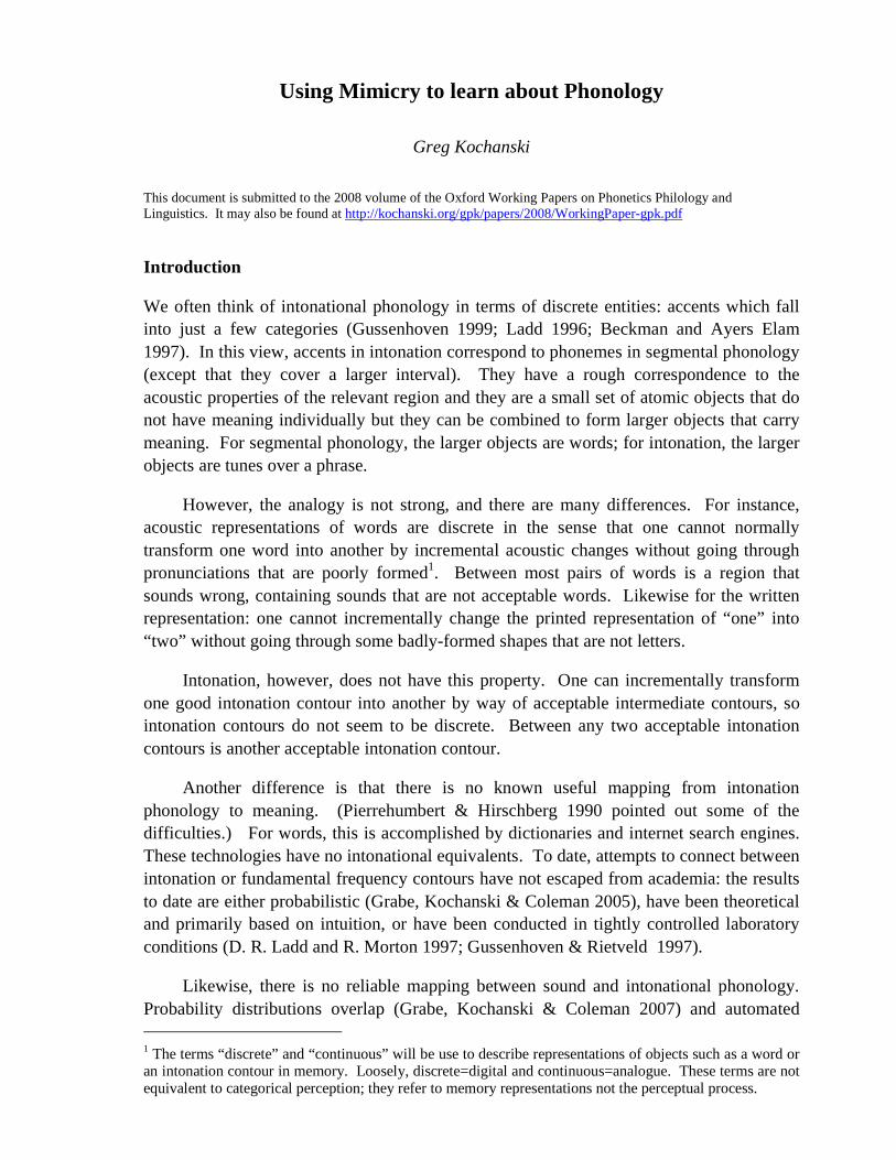
Figure 1 shows a simple model of mimicry. This model treats mimicry as a completely normal speech process: a person hears speech, perceives it, and generates a memory representation for it. Later, the person produces speech from the memory. Most contentious point might be the identification of the memory representation with a phonological representation. But, if people don’t produce speech from phonological entities2, what is the relevance of linguistics? Likewise, if phonological entities are not the end-product of the perceptual process, where do they come from?3 It is certainly not satisfactory to divorce phonology from behaviour and perception because phonological entities are not directly observable, so we can only study phonology by aiming sounds at people and observing what they do4.

2 Or, more precisely, “If we cannot usefully predict the acoustic properties of speech from phonology…” 3 Of course, the perceptual process can be described at various levels of detail, and phonology is only one level of description. However, for phonology to be meaningful, there must eventually be a consistent description of the perceptual process (ideally, a quantitative, numerical model) that takes acoustics on one side and yields phonological entities on the other side. 4 And, one of those behaviours, especially common among linguists, is to speak, describing the sounds in terms of phonological entities.

Sound Perception Memory Production Sound

Domain of phonology

Figure 1: Mimicry via phonology. Sound is perceived, stored in memory in some phonological representation, then when the subject begins to speak, he or she articulates based on the stored memory representation.

Other models of mimicry are possible, but they lead to a more complex overall description of human behaviour. For instance, if mimicry were a hard-wired part of early language learning, one might imagine that there were two separate parallel channels, one for non-phonological mimicry and one for speech that is treated phonologically. However, such a model would be more complex and evidence for a separate channel is weak5.

If we assume Figure 1, the critical question then becomes the nature of the memory trace. Is it continuous in the sense that a small change in fundamental frequency always corresponds to a small change in the memory representation? This would imply that memory stores something much like pitch, suggesting some variety of Exemplar model (Pierrehumbert 2001). Or, alternatively, is the memory representation could be discrete, leading to a model with a model close to Generative Phonology (e.g. Liberman 1970). These two hypotheses will be considered below.

Below, I follow standard practice and approximate intonation by measurements of speech fundamental frequency. This is undoubtedly incomplete: for instance loudness and duration are important in defining accent locations (Kochanski et al 2005, Kochanski 2006 and references therein).

5 Most arguments for a separate mimicry channel assumes that the phonological channel is strictly discrete. Under that assumption, then early learning of speech before phonology is well-established, demands a specialised mimicry channel. However, in the context of this paper, we are not assuming that phonology is discrete so this assumption becomes circular.

Memory Production Sound

Domain of phonology

f0 f0

Hypothesis 1: memory stores an acoustic trace

Continuous

Sound Perception

Figure 2: Hypothetical model of mimicry where the memory store is continuous. The lower half of the drawing represents speech fundamental frequency (increasing upwards) at some point in a phrase. The lines connect input fundamental frequency (left axis) to the corresponding memory representation (centre) to the fundamental frequency that is eventually produced (right axis).

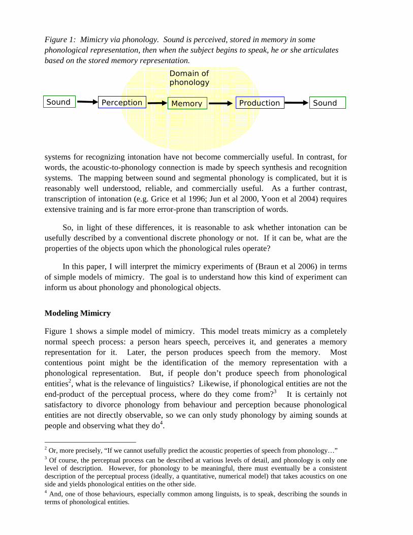
Hypothesis 1: The memory store is a continuous representation of fundamental frequency.

In this hypothesis (Figure 2) nearby values of speech fundamental frequency in the input utterance are represented by nearby memory representations. Further, nearby memory representations yield nearby fundamental frequencies in the speech that is eventually produced. In other words, there is a continuous mapping between input fundamental frequency and the memory representation, a continuous memory representation, and a continuous mapping on the output.

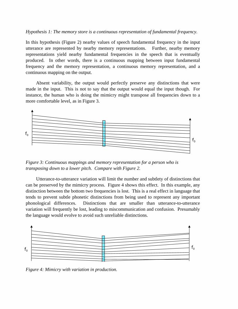
Absent variability, the output would perfectly preserve any distinctions that were made in the input. This is not to say that the output would equal the input though. For instance, the human who is doing the mimicry might transpose all frequencies down to a more comfortable level, as in Figure 3.

Utterance-to-utterance variation will limit the number and subtlety of distinctions that can be preserved by the mimicry process. Figure 4 shows this effect. In this example, any distinction between the bottom two frequencies is lost. This is a real effect in language that tends to prevent subtle phonetic distinctions from being used to represent any important phonological differences. Distinctions that are smaller than utterance-to-utterance variation will frequently be lost, leading to miscommunication and confusion. Presumably the language would evolve to avoid such unreliable distinctions.

f0

f0

Figure 3: Continuous mappings and memory representation for a person who is transposing down to a lower pitch. Compare with Figure 2.

f0 f0

Figure 4: Mimicry with variation in production.

However, while language users are limited by variation, laboratory experiments need not be. Experiments can average over many utterances (a luxury that language users don’t have in the midst of a conversation), reducing the variation as much as needed. If we do so, we can construct an ideal variation-free model such as Figure 5. In that model, all input distinctions are preserved through the memory representation to the output.

Hypothesis 0: The memory store is discrete

The null hypothesis for the field of Intonational Phonology is different. Intonational Phonology, like most of linguistics, assumes that the phonology can be represented well by discrete symbols. For the sake of argument, we assume that we can find a minimal pair of intonation contours that differ only by a single symbol, H vs. L6. Figure 6 shows this hypothesis schematically. The intonation is perceived (either categorically or not), then stored in memory as one or the other of two discrete representations. Finally, when the subject mimics the intonation contour, his/her speech is produced from the memory representation.

6 However, the argument presented here does not depend upon having a minimal pair or upon having a simple difference. We will merely assume that there are a finite number of discrete memory representations. We also assume that these memory representations are not so numerous that perception is ambiguous.

f0 f0

Figure 5: ideal model obtained by averaging results from many utterances to reduce variation. In this model of mimicry, all input distinctions are preserved and appear in the output. The pair of coloured lines show a distinction between two slightly different utterances. At some point, these utterances have different fundamental frequency (left), which is perceived as two different memory representations (centre). These different memory representations lead to a measurable difference in the fundamental frequency that the subject produces (right).

Now, on the basis of an individual utterance, production variation will yield a broad range of outputs for each memory representation. Figure 7 shows several potential outputs from the same phonology. Potentially, the resulting probability distributions produced from H and L could even overlap (though any substantial overlap would mean that the H vs. L distinction was not sufficiently clear to form a minimal pair).

However, just as with Hypothesis 1, we can average over all productions from the same phonology and remove the effect of the variation. In this case, we see that the averaged productions form two well-separated values, different for H and L. However, the crucial difference between Hypotheses 0 and 1 lies in which distinctions are preserved. Hypothesis 1 preserves all input distinctions through to the output, but that is not the case for Hypothesis 0.

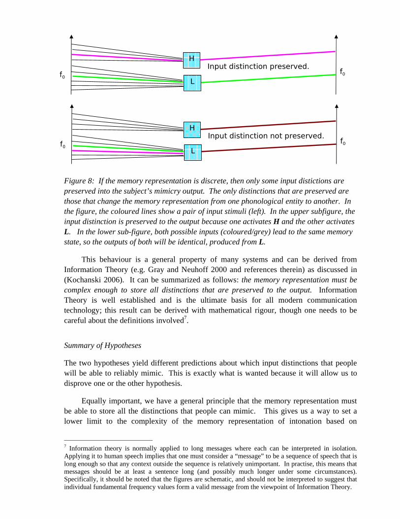
Figure 8 shows that distinctions between phonological entities are preserved but not input distinctions that produce the same phonological entity. In other words, any inputs that yield the same memory representation will produce the same output; distinctions within those sets are lost.

f0 f0

H

L

f f

H

L

f f

H

Lf f

H

Lf f

H

L

Figure 6: Hypothetical model of mimicry where the memory store is discrete. The drawing represents speech fundamental frequency (increasing upwards) at some point in a phrase. The lines connect input fundamental frequency (left axis) to the corresponding memory representation (centre) to the fundamental frequency that is eventually produced (right axis).

Figure 7: Several productions from the same phonology. The sub-figures show production variation.

This behaviour is a general property of many systems and can be derived from Information Theory (e.g. Gray and Neuhoff 2000 and references therein) as discussed in (Kochanski 2006). It can be summarized as follows: the memory representation must be complex enough to store all distinctions that are preserved to the output. Information Theory is well established and is the ultimate basis for all modern communication technology; this result can be derived with mathematical rigour, though one needs to be careful about the definitions involved7.

Summary of Hypotheses

The two hypotheses yield different predictions about which input distinctions that people will be able to reliably mimic. This is exactly what is wanted because it will allow us to disprove one or the other hypothesis.

Equally important, we have a general principle that the memory representation must be able to store all the distinctions that people can mimic. This gives us a way to set a lower limit to the complexity of the memory representation of intonation based on

7 Information theory is normally applied to long messages where each can be interpreted in isolation. Applying it to human speech implies that one must consider a “message” to be a sequence of speech that is long enough so that any context outside the sequence is relatively unimportant. In practise, this means that messages should be at least a sentence long (and possibly much longer under some circumstances). Specifically, it should be noted that the figures are schematic, and should not be interpreted to suggest that individual fundamental frequency values form a valid message from the viewpoint of Information Theory.

f0 f0

H

L

Input distinction not preserved.

f0 f0

H

L

Input distinction preserved.

Figure 8: If the memory representation is discrete, then only some input distictions are preserved into the subject’s mimicry output. The only distinctions that are preserved are those that change the memory representation from one phonological entity to another. In the figure, the coloured lines show a pair of input stimuli (left). In the upper subfigure, the input distinction is preserved to the output because one activates H and the other activates L. In the lower sub-figure, both possible inputs (coloured/grey) lead to the same memory state, so the outputs of both will be identical, produced from L.

observations of human behaviour. This allows us to experimentally measure at least one property of phonological entities.

Experiments on the Intonation of Speech

The experiments discussed here have been reported in (Kochanski et al 2005). The goal of this paper is not to present the data again, but rather to interpret it in the light of Hypotheses 0 and 1 to see what can be learned about human memory for intonation.

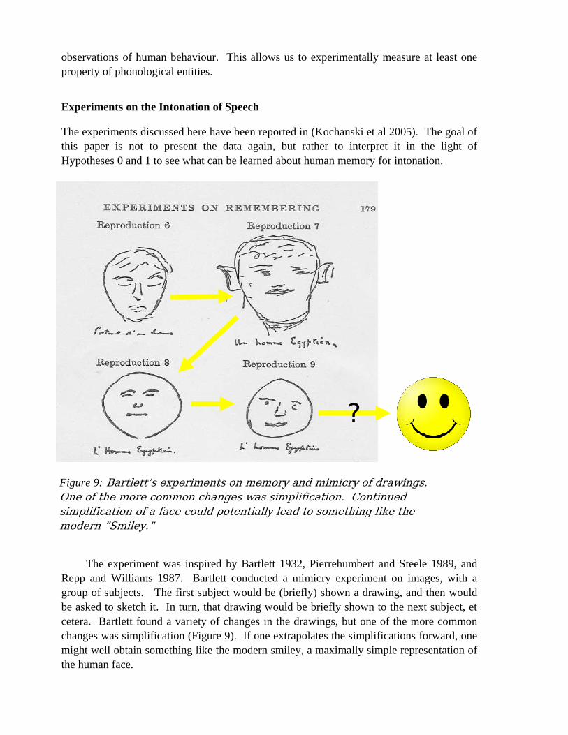
The experiment was inspired by Bartlett 1932, Pierrehumbert and Steele 1989, and Repp and Williams 1987. Bartlett conducted a mimicry experiment on images, with a group of subjects. The first subject would be (briefly) shown a drawing, and then would be asked to sketch it. In turn, that drawing would be briefly shown to the next subject, et cetera. Bartlett found a variety of changes in the drawings, but one of the more common changes was simplification (Figure 9). If one extrapolates the simplifications forward, one might well obtain something like the modern smiley, a maximally simple representation of the human face.

?

Figure 9: Bartlett’s experiments on memory and mimicry of drawings.

One of the more common changes was simplification. Continued

simplification of a face could potentially lead to something like the

modern “Smiley.”

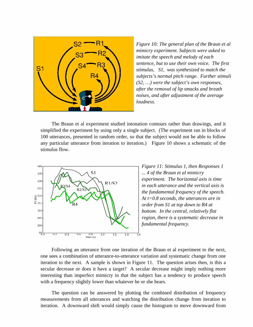
The Braun et al experiment studied intonation contours rather than drawings, and it simplified the experiment by using only a single subject. (The experiment ran in blocks of 100 utterances, presented in random order, so that the subject would not be able to follow any particular utterance from iteration to iteration.) Figure 10 shows a schematic of the stimulus flow.

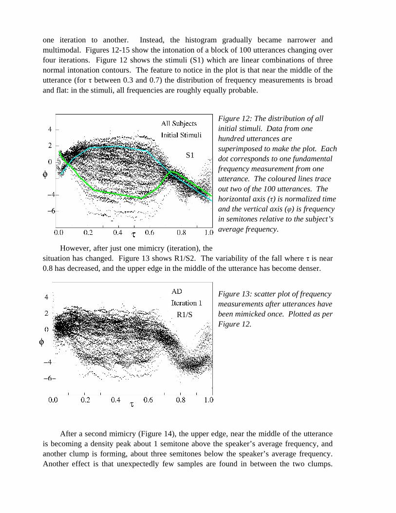
Following an utterance from one iteration of the Braun et al experiment to the next, one sees a combination of utterance-to-utterance variation and systematic change from one iteration to the next. A sample is shown in Figure 11. The question arises then, is this a secular decrease or does it have a target? A secular decrease might imply nothing more interesting than imperfect mimicry in that the subject has a tendency to produce speech with a frequency slightly lower than whatever he or she hears.

The question can be answered by plotting the combined distribution of frequency measurements from all utterances and watching the distribution change from iteration to iteration. A downward shift would simply cause the histogram to move downward from

Figure 10: The general plan of the Braun et al mimicry experiment. Subjects were asked to imitate the speech and melody of each sentence, but to use their own voice. The first stimulus, S1, was synthesized to match the subjects’s normal pitch range. Further stimuli (S2, …) were the subject’s own responses, after the removal of lip smacks and breath noises, and after adjustment of the average loudness.

S1

R1/S2 R2/S3

R3/S4

R4

Figure 11: Stimulus 1, then Responses 1 ... 4 of the Braun et al mimicry experiment. The horizontal axis is time in each utterance and the vertical axis is the fundamental frequency of the speech. At t=0.8 seconds, the utterances are in order from S1 at top down to R4 at bottom. In the central, relatively flat region, there is a systematic decrease in fundamental frequency.

one iteration to another. Instead, the histogram gradually became narrower and multimodal. Figures 12-15 show the intonation of a block of 100 utterances changing over four iterations. Figure 12 shows the stimuli (S1) which are linear combinations of three normal intonation contours. The feature to notice in the plot is that near the middle of the utterance (for τ between 0.3 and 0.7) the distribution of frequency measurements is broad and flat: in the stimuli, all frequencies are roughly equally probable.

However, after just one mimicry (iteration), the situation has changed. Figure 13 shows R1/S2. The variability of the fall where τ is near 0.8 has decreased, and the upper edge in the middle of the utterance has become denser.

After a second mimicry (Figure 14), the upper edge, near the middle of the utterance is becoming a density peak about 1 semitone above the speaker’s average frequency, and another clump is forming, about three semitones below the speaker’s average frequency. Another effect is that unexpectedly few samples are found in between the two clumps.

Figure 12: The distribution of all initial stimuli. Data from one hundred utterances are superimposed to make the plot. Each dot corresponds to one fundamental frequency measurement from one utterance. The coloured lines trace out two of the 100 utterances. The horizontal axis (τ) is normalized time and the vertical axis (φ) is frequency in semitones relative to the subject’s average frequency.

Figure 13: scatter plot of frequency measurements after utterances have been mimicked once. Plotted as per Figure 12.

S1

R1/S2

The region where τ is near 0.25, one to two semitones below the speaker’s average is becoming sparse.

Finally, after four mimicries, Figure 15 shows that two separate groups of intonation contours have formed in the central part of the utterance. Utterances with intermediate frequencies have almost disappeared.

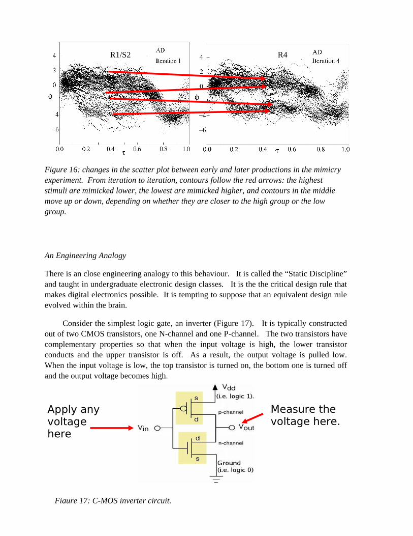
What is happening is that every time an utterance is mimicked, the produced intonation contour is biased towards one or the other of these two groups of contours. Figure 16 shows this by comparing an early and a late production. Aside from a certain amount of random variation, the contours approach either a high target or a low target, whichever they are closest to. In mathematical terms, from one iteration to the next, the contours are mapped towards one of these two attractors.

Figure 14: scatter plot of fundamental frequency measurements after two mimicries. Plotted as per Figure 12.

R4

R2/S3

Figure 15: The scatterplot at the end of the experiment, after four mimicries. Plotted as per Figure 12. The blue line marks one utterance’s intonation contour.

An Engineering Analogy

There is an close engineering analogy to this behaviour. It is called the “Static Discipline” and taught in undergraduate electronic design classes. It is the the critical design rule that makes digital electronics possible. It is tempting to suppose that an equivalent design rule evolved within the brain.

Consider the simplest logic gate, an inverter (Figure 17). It is typically constructed out of two CMOS transistors, one N-channel and one P-channel. The two transistors have complementary properties so that when the input voltage is high, the lower transistor conducts and the upper transistor is off. As a result, the output voltage is pulled low. When the input voltage is low, the top transistor is turned on, the bottom one is turned off and the output voltage becomes high.

R1/S2 R4

Apply any voltage here

Measure the voltage here.

Figure 17: C-MOS inverter circuit.

Figure 16: changes in the scatter plot between early and later productions in the mimicry experiment. From iteration to iteration, contours follow the red arrows: the highest stimuli are mimicked lower, the lowest are mimicked higher, and contours in the middle move up or down, depending on whether they are closer to the high group or the low group.

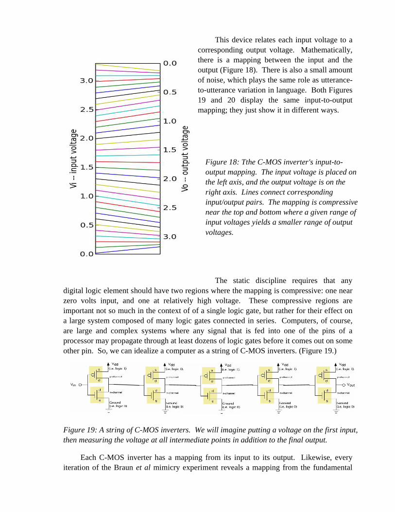
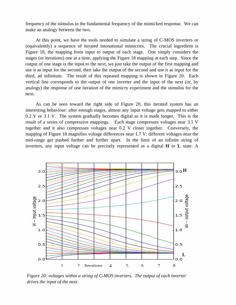
This device relates each input voltage to a corresponding output voltage. Mathematically, there is a mapping between the input and the output (Figure 18). There is also a small amount of noise, which plays the same role as utterance-to-utterance variation in language. Both Figures 19 and 20 display the same input-to-output mapping; they just show it in different ways.

The static discipline requires that any digital logic element should have two regions where the mapping is compressive: one near zero volts input, and one at relatively high voltage. These compressive regions are important not so much in the context of of a single logic gate, but rather for their effect on a large system composed of many logic gates connected in series. Computers, of course, are large and complex systems where any signal that is fed into one of the pins of a processor may propagate through at least dozens of logic gates before it comes out on some other pin. So, we can idealize a computer as a string of C-MOS inverters. (Figure 19.)

Each C-MOS inverter has a mapping from its input to its output. Likewise, every iteration of the Braun et al mimicry experiment reveals a mapping from the fundamental

Figure 18: Tthe C-MOS inverter's input-to-output mapping. The input voltage is placed on the left axis, and the output voltage is on the right axis. Lines connect corresponding input/output pairs. The mapping is compressive near the top and bottom where a given range of input voltages yields a smaller range of output voltages.

Figure 19: A string of C-MOS inverters. We will imagine putting a voltage on the first input, then measuring the voltage at all intermediate points in addition to the final output.

frequency of the stimulus to the fundamental frequency of the mimicked response. We can make an analogy between the two.

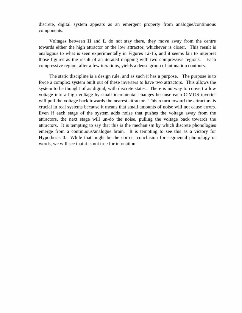
At this point, we have the tools needed to simulate a string of C-MOS inverters or (equivalently) a sequence of iterated intonational mimicries. The crucial ingredient is Figure 18, the mapping from input to output of each stage. One simply considers the stages (or iterations) one at a time, applying the Figure 18 mapping at each step. Since the output of one stage is the input to the next, we just take the output of the first mapping and use it as input for the second, then take the output of the second and use it as input for the third, ad infinitum. The result of this repeated mapping is shown in Figure 20. Each vertical line corresponds to the output of one inverter and the input of the next (or, by analogy) the response of one iteration of the mimicry experiment and the stimulus for the next.

As can be seen toward the right side of Figure 20, this iterated system has an interesting behaviour: after enough stages, almost any input voltage gets mapped to either 0.2 V or 3.1 V. The system gradually becomes digital as it is made longer. This is the result of a series of compressive mappings. Each stage compresses voltages near 3.1 V together and it also compresses voltages near 0.2 V closer together. Conversely, the mapping of Figure 18 magnifies voltage differences near 1.7 V: different voltages near the mid-range get pushed further and further apart. In the limit of an infinite string of inverters, any input voltage can be precisely represented as a digital H or L state. A

Figure 20: voltages within a string of C-MOS inverters. The output of each inverter drives the input of the next.

H

L

1 2 Iterations 4 5 6 7 8

discrete, digital system appears as an emergent property from analogue/continuous components.

Voltages between H and L do not stay there, they move away from the centre towards either the high attractor or the low attractor, whichever is closer. This result is analogous to what is seen experimentally in Figures 12-15, and it seems fair to interpret those figures as the result of an iterated mapping with two compressive regions. Each compressive region, after a few iterations, yields a dense group of intonation contours.

The static discipline is a design rule, and as such it has a purpose. The purpose is to force a complex system built out of these inverters to have two attractors. This allows the system to be thought of as digital, with discrete states. There is no way to convert a low voltage into a high voltage by small incremental changes because each C-MOS inverter will pull the voltage back towards the nearest attractor. This return toward the attractors is crucial in real systems because it means that small amounts of noise will not cause errors. Even if each stage of the system adds noise that pushes the voltage away from the attractors, the next stage will un-do the noise, pulling the voltage back towards the attractors. It is tempting to say that this is the mechanism by which discrete phonologies emerge from a continuous/analogue brain. It is tempting to see this as a victory for Hypothesis 0. While that might be the correct conclusion for segmental phonology or words, we will see that it is not true for intonation.

Discussion

Intonational Attractors are Slow

We saw already that it took several iterations of the mimicry experiment for the intonation contours to approach the high and low attractors. This can be quantified by measuring how strongly bimodal is each scatter-plot of fundamental frequency (e.g. Figure 15). Without going into the details which can be found in Braun et al, the results can be seen in Figure 21. The scatter-plots become more strongly bimodal as the experiment progresses, but it happens slowly, over several iterations. Recall that each iteration is a complete pass through the human subject involving on the order of 100 stages where one neuron triggers another, so if we equate a logic gate with a few neurons, the rate of convergence per group of neurons (i.e. per logic gate) must be small indeed.

More practically, if it takes roughly four iterations for the fundamental frequency to converge toward a pair of almost-discrete states, then one certainly should not expect digital behaviour to emerge on a single trip between the ears and memory. The

Figure 21: Answer to the question “How strongly bi-modal is the frequency distribution?” The vertical axis (valley depth) measures the how empty is the middle of the scatterplot (e.g. Figure 15), relative to the density of fundamental frequency measurements near the high and low attractors. A value of zero implies that there is only a single peak; one corresponds to strongly overlapping peaks; values over two correspond to two well-separated peaks. The horizontal axis shows the number of experimental iterations. Each curve corresponds to a different experimental subject. The gradual increase in valley depth values implies a slow and gradual separation of the scatter-plots into two peaks ( except for one subject who seemed unable to mimic at all).

convergence that we see is approximately ten times too slow for intonational phonology to be accurately represented by a discrete memory representation.

What is stored in the memory representation?

One should also consider which distinctions the subjects can mimic. Recall that the memory representation must be at least rich enough to store all the distinctions that can be mimicked. A comparison of Figures 12 and 13 shows that subjects are able to mimic fine phonetic detail fairly accurately. Not only can subjects reproduce the contours that happen to be near the attractors, but they can reproduce the extreme contours and the contours half-way between the attractors, too. So, all this detail is stored in memory and is plausibly part of the phonological entities.

Hypothesis 1 is actually the better approximation to our data, at least over a single iteration. All input distinctions are carried through to the output, although some distinctions may be emphasized and others reduced. Figure 22 shows one reasonable interpretation for mimicry behaviour. This model takes the view that the memory representation is essentially an acoustic memory, but biased slightly toward one or another special intonation contours. If interpreted literally, this model suggests that intonation contours are stored in something like the phonological loop (Baddeley 1997) and the gentle bias toward the attractors is due to interactions something stable outside the phonological loop.

Another reasonable interpretation that is closer to the traditional phonological approach is to consider the memory to be a discrete phonological symbol along with substantial amounts of fine phonetic detail. This is a sort of “decorated object”, shown in Figure 23. However, this interpretation does not carry a license to do traditional discrete phonology. We know that the fine phonetic detail is there, stored in the memory representation, so one cannot arbitrarily ignore it. A proper phonological theory would include it, would involve it in the computations, and presumably, the fine phonetic detail would affect the answer generated in some phonological computations.

f0 f0

EXAGGERATE

ERODE

ERODE

Figure 22: A plausible interpretation of the mimicry results, corresponding to an intermediate case between Hypothesis 0 and Hypothesis 1. All distinctions are preserved, but some are partially eroded and others are emphasised.

Given that some fine phonetic detail is stored, the onus is on the phonologists to show

that their computations are useful approximations to human language behaviour. Any phonological theory that uses discrete objects carries a hidden assumption that such discrete representations actually exist in the mind. This is a strong assumption and needs to be justified, otherwise the resulting theory is built on sand.

Especially since we know the fine phonetic detail is used by some phonological processes, because we can hear the detail when a subject mimics an intonation contour. The phonological processes of speech production do not limit themselves to using the strictly discrete part of a decorated object. They use both the discrete part and the fine phonetic decoration, and presumably other phonological processes also do so. It will be a challenge for theorists to re-cast phonology in terms of either of these interpretations.

Conclusion

A straightforward interpretation of results from mimicry experiments shows interesting, complicated behaviour. The existence of attractors in intonation and their similarity to common intonation contours suggests that something like intonational phonology exists. However, the approach toward the attractors is far too slow for discrete phonological categories to be a good approximation to the way humans actually remember and reproduce intonation. To the extent that discrete phonological entities exist for intonation, they have only a weak influence on actual behaviour.

Humans do not behave as if their memory representation of intonation were a few discrete states. Memory certainly captures a much richer set of distinctions than two phonological categories, and a reasonable interpretation is that a substantial amount of detailed information about the intonation contour is stored in memory, available for processing. Further, this detailed information is actually used in the mental processes of speech production.

Acknowlegment

The beginnings of this work were been funded by the Oxford University Research Development fund and later stages by the UK’s Economic and Social Research Council under grant RES-000-23-1094. Both were greatly appreciated.

f0 f0

Figure 23: A plausible interpretation of mimicry results in terms of decorated categories or decorated symbols.

References

Baddeley, A. (1997) Human Memory: Theory and Practice (Revised Edition), Psychology Press, Hove, East Sussex, UK. ISBN 0-86377-431-8.

Bartlett, F. C. (1932), Remembering, Cambridge University Press, Cambridge.

Beckman, M. & Ayers Elam, G. (1997) Guidelines for ToBI labeling, Linguistics Department, Ohio State University, http://ling.ohio-state-edu/~tobi/ame_tobi/labelling_guide_v3.pdf

Braun, B., Kochanski, G., Grabe, E. & Rosner, B. (2006) ‘Evidence for attractors in English intonation’, J. Acoustical Society of America 119(6): 4006-4015, doi:10.1121/1.2195267

Grabe, E., Kochanski, G. & Coleman, J. (2005), ‘The intonation of native accent varieties in the British Isles – Potential for miscommunication?’ in K. Dziubalska-Kolaczyk and J. Przedlacka (eds) English pronunciation models: A changing scene. Linguistic Insights Series 21, Peter Lang (Oxford, Berlin, New York), ISBN 3-03910-662-7, US-ISBN 0-8204-7173-9.

Grabe, E., Kochanski, G. & Coleman, J. (2007), ‘Connecting Intonation Labels to Mathematical Descriptions of Fundamental Frequency,’ Language and Speech, 50 (3): 281-310.

Gray, R. M. & Neuhoff, D. L. (2000) ‘Quantization’ in Information Theory: 50 years of discovery, S. Verdú (ed), IEEE Press, Piscataway NJ. Reprinted from IEEE Transactions of Information Theory 4: (1998).

Grice, M., Reyelt, M., Benzmüller, R., Mayer, J. & Batliner, R. (1996), ‘Consistency of transcription and labelling of German intonation with GToBI’, Proceedings of the Fourth International Conference on Spoken Language Processing (ICSLP) 1716-1719, Philadelphia, PA.

Gussenhoven, C. ‘Discreteness and Gradience in Intonational Contrasts’ (1999) Language and Speech, 42(2-3): 283-305.

Gussenhoven, C. & Rietveld, A. M. C. (1997), ‘Empirical evidence for the contrast between Dutch rising intonation contours’, in A. Botinis, G. Kouroupetroglou, and G. Carayiannis, Intonation: Theory, Models and Applications, Proceedings of an ESCA Tutorial and Research Workshop, Athens, Greece, September 18-20.

Jun, S. –A., Sook-Hyang, L., Keeho, K. & Yong-Ju, L. (2000) ‘Labeler agreement in transcribing Korean intonation with K-ToBI’, Proceedings of the Sixth International Conference on Spoken Language Processing (ICSLP), Beijing, China.

Kochanski, G. (2006) ‘Prosody beyond fundamental frequency’ in Methods in Empirical Prosody Research, S. Sudhoff, P. Augurzky, I. Mleinek and N. Richter, eds. De Gruyter; Language, Context and Cognition Series (Berlin, New York). ISBN 3-11-018856-2.

Kochanski, G., Grabe, E., Coleman, J. & Rosner, B. (2005) ‘Loudness predicts prominence: fundamental frequency lends little’, J. Acoustic Society of America 118(2): 1038-1054. doi:10.1121/1.1923349.

Ladd, D. R. (1996) Intonational Phonology, Cambridge Studies in Linguistics, Cambridge University Press, Cambridge UK. ISBN 0-521-47498-1.

Ladd, D. R. & Moreton, R. (1997) ‘The perception of intonational emphasis: continuous or categorical?’ J. of Phonetics 25: 313-342.

Liberman, A. M. ‘The grammars of speech and language’ (1970), Cognitive Psychology (1): 301-323.

Pierrehumbert, J. ‘Exemplar dynamics: Word frequency, lenition and contrast’ (2001) in Frequency and the Emergence of Linguistic Structure, J. Bybee and P.Hopper, eds. Benjamins, Amsterdam.

Pierrehumbert J. & Hirschberg, J. (1990) ‘The meaning of intonation contours in the interpretation of discourse.’ In P. R. Cohen, J. Morgan and M. E. Pollack (eds), Proceedings of the Third International Conference on Spoken Language Processing (ICSLP), v. 2: 123-126, Yokohama.

Pierrehumbert, J. & Steele, S. A. (1989) ‘Categories of tonal alignment in English,’ Phonetica 46: 181-196.

Repp, B. H. & Williams, D. R. (1987) ‘Categorical tendencies in self-imitating self-produced vowels’, Speech Communication 6: 1-14.

Yoon, T., Chavarria, S., Cole, J. & Hasegawa-Johnson, M. (2004), ‘Intertranscriber reliability of prosodic labeling on telephone conversation using ToBI’, Proceedings of the ICSA International Conference on Spoken :Language Processing (Interspeech 2004), 2729-2732, Jeju, Korea.