USING MATHEMATICAL MODEL TO

ILLUSTRATE THE SPREAD OF MALARIA

Kiyeny Silas Kipchirchir

July 2014

1

Abstract

We present an ordinary differential equation mathematical model for

the spread of malaria in human and Mosquito populations.Susceptible

humans can be infected when the are bitten by an infectious Mosquito.They

then progress through the infectious and asymptomatic classes, before

re-entering the susceptible class.Susceptible Mosquitoes can become

infected when they bite infectious and asymptomatic humans, and

once infected they move through infectious class. The basic repro-

duction number R0 is established and used to determine whether the

disease dies out or persists in the population. We show that given

R0 ≤ 1, the disease-free equilibrium is globally asymptotically stable

and the disease always dies out and if R0 > 1, there exists a unique

endemic equilibrium which is globally stable and the disease persists.

2

Contents

1 INTRODUCTION 5

1.1 Malaria . . . . . . . . . . . . . . . . . . . . . . . . . . . . . . 5

1.2 Causes of malaria . . . . . . . . . . . . . . . . . . . . . . . . . 7

1.3 Life cycle of Plasmodium and how malaria spreads . . . . . . 8

1.4 Signs and Symptoms of Malaria . . . . . . . . . . . . . . . . . 10

1.5 Asymptomatic malaria . . . . . . . . . . . . . . . . . . . . . . 11

1.6 Mathematical models and epidemiology . . . . . . . . . . . . . 13

1.7 Problem Statement . . . . . . . . . . . . . . . . . . . . . . . . 14

1.8 Objectives of the study . . . . . . . . . . . . . . . . . . . . . . 15

1.8.1 Specific objectives . . . . . . . . . . . . . . . . . . . . . 15

2 LITERATURE REVIEW 16

2.1 History of Malaria . . . . . . . . . . . . . . . . . . . . . . . . 16

2.2 Mathematical modeling of malaria . . . . . . . . . . . . . . . . 20

3 MODEL DESCRIPTION AND ANALYSIS 27

3.1 Model formulation . . . . . . . . . . . . . . . . . . . . . . . . 27

3.2 Model analysis . . . . . . . . . . . . . . . . . . . . . . . . . . 32

3.3 A compact positively invariant set . . . . . . . . . . . . . . . . 37

3.4 Reduction of the model . . . . . . . . . . . . . . . . . . . . . . 38

3.5 The Basic Reproduction Number . . . . . . . . . . . . . . . . 40

3.6 Stability analysis . . . . . . . . . . . . . . . . . . . . . . . . . 47

3

3.6.1 Disease Free Equilibrium (DFE), E0 . . . . . . . . . . 47

3.6.2 Local stability analysis of the DFE,E0 . . . . . . . . . 48

3.6.3 Global stability analysis of the DFE, E0 . . . . . . . . 54

3.6.4 Endemic equilibrium . . . . . . . . . . . . . . . . . . . 57

3.6.5 Local stability analysis of the endemic equilibrium EE,E1 64

3.7 Numerical simulations . . . . . . . . . . . . . . . . . . . . . . 70

4 CONCLUSION 73

4

1 INTRODUCTION

1.1 Malaria

Malaria is an ancient disease having huge social, economic and health burden.

It is predominantly present in the tropical countries. Even though the disease

has been investigated for hundreds of years, it still remains a major public

health problem. The WHO estimates that in 2010 there were 219 million

cases of malaria resulting in 660,000 deaths [1,2]. Others have estimated the

number of cases at between 350 and 550 million for falciparum malaria [3] and

deaths in 2010 at 1.24 million [4] up from 1.0 million deaths in 1990 [5]. The

majority of cases (65 percent) occur in children under 15 years old [4]. About

125 million pregnant women are at risk of infection each year; in Sub-Saharan

Africa, maternal malaria is associated with up to 200,000 estimated infant

deaths yearly [6]. There are about 10,000 malaria cases per year in Western

Europe, and 1300-1500 in the United States [7]. About 900 people died from

the disease in Europe between 1993 and 2003 [8]. Both the global incidence

of disease and resulting mortality have declined in recent years. According

to WHO, deaths attributable to malaria in 2010 were reduced by over a

third from a 2000 estimate of 985,000, largely due to the widespread use of

insecticide-treated nets and artemisinin-based combination(ACT) therapies

[9].

Malaria is presently endemic in a broad band around the equator, in areas

5

of the Americas, many parts of Asia, and much of Africa; 85-90 percent

of malaria fatalities occur in Sub-Saharan Africa [10]. An estimate for 2009

reported that countries with the highest death rate per 100,000 of population

were Ivory Coast (86.15), Angola (56.93) and Burkina Faso (50.66) [11]. A

2010 estimate indicated the deadliest countries per population were Burkina

Faso, Mozambique and Mali [4]. The Malaria Atlas Project aims to map

global endemic levels of malaria, providing a means with which to determine

the global spatial limits of the disease and to assess disease burden [12,13].

This effort led to the publication of a map of P. falciparum endemicity in

2010 [20]. As of 2010, about 100 countries have endemic malaria [2,14]. Every

year, 125 million international travellers visit these countries, and more than

30,000 contract the disease [8].

The geographic distribution of malaria within large regions is complex, and

malaria-afflicted and malaria-free areas are often found close to each other

[15]. Malaria is prevalent in tropical and subtropical regions because of rain-

fall, consistent high temperatures and high humidity, along with stagnant

waters in which mosquito larvae readily mature, providing them with the en-

vironment they need for continuous breeding [16]. In drier areas, outbreaks

of malaria have been predicted with reasonable accuracy by mapping rainfall

[17]. Malaria is more common in rural areas than in cities. For example, sev-

eral cities in the Greater Mekong Subregion of Southeast Asia are essentially

malaria-free, but the disease is prevalent in many rural regions, including

along international borders and forest fringes [18]. In contrast, malaria in

6

Africa is present in both rural and urban areas, though the risk is lower in

the larger cities [19].

1.2 Causes of malaria

Malaria is caused by Plasmodium parasite which can be spread to humans

through the bites of an infected Mosquitoes. There are many different types

of Plasmodium parasite, but only five types cause malaria in humans [21,22].

These are:

• Plasmodium falciparum- mainly found in Africa and responsible for

most malaria deaths worldwide.

• Plasmodium vivax - mainly found in Asia and Latin America. This

parasite produces less severe symptoms than Plasmodium falciparum,

but it can stay in the liver for up to three years, which can result in

relapses.

• Plasmodium Ovale-fairly uncommon and usually found in west Africa.

It can remain in human liver for several years without producing symp-

toms.

• Plasmodium Malariae- this is quite rare and usually found in Africa.

• Plasmodium Knowlesi - this is very rare and found in parts of Southeast

Asia.

7

Of these Plasmodium falciparum is the most common cause of infection in

Africa and Southeast Asia, and is responsible for approximately 80 percent

of all malaria cases and approximately 90 percent of deaths [1].

1.3 Life cycle of Plasmodium and how malaria spreads

In the life cycle of Plasmodium, a female Anopheles mosquito (the definitive

host) transmits a motile infective form (called the sporozoite) to a vertebrate

host such as a human (the secondary host), thus acting as a transmission

vector. A sporozoite travels through the blood vessels to liver cells (hepa-

tocytes), where it reproduces asexually (tissue schizogony), producing thou-

sands of merozoites. These infect new red blood cells and initiate a series of

asexual multiplication cycles (blood schizogony) that produce 8 to 24 new

infective merozoites, at which point the cells burst and the infective cycle

begins a new [23].

Other merozoites develop into immature gametocytes, which are the pre-

cursors of male and female gametes. When a fertilised mosquito bites an

infected person, gametocytes are taken up with the blood and mature in the

mosquito gut. The male and female gametocytes fuse and form a ookinetea

fertilized, motile zygote. Ookinetes develop into new sporozoites that mi-

grate to the insect’s salivary glands, ready to infect a new vertebrate host.

The sporozoites are injected into the skin, in the saliva, when the mosquito

takes a subsequent blood meal [24].

8

Only female mosquitoes feed on blood; male mosquitoes feed on plant nectar,

and thus do not transmit the disease. The females of the Anopheles genus

of mosquito prefer to feed at night. They usually start searching for a meal

at dusk, and will continue throughout the night until taking a meal [25].

Malaria parasites can also be transmitted by blood transfusions, although

this is rare [26]

9

Figure 1: Life cycle of Plasmodium parasite

1.4 Signs and Symptoms of Malaria

The signs and symptoms of malaria typically begin 8-25 days following infec-

tion [27]; however, symptoms may occur later in those who have taken anti-

malarial medications as prevention [1]. Initial manifestations of the disease-

common to all malaria species-are similar to flu-like symptoms [28], and can

resemble other conditions such as septicemia, gastroenteritis, and viral dis-

eases [1]. The presentation may include headache, fever, shivering, joint

10

pain, vomiting, hemolytic anemia, jaundice, hemoglobin in the urine, retinal

damage, and convulsions [29].

The classic symptom of malaria is paroxysm-a cyclical occurrence of sudden

coldness followed by shivering and then fever and sweating, occurring every

two days (tertian fever) in P. vivax and P. ovale infections, and every three

days (quartan fever) for P. malariae. P. falciparum infection can cause re-

current fever every 36-48 hours or a less pronounced and almost continuous

fever [30].

Severe malaria is usually caused by P. falciparum (often referred to as fal-

ciparum malaria). Symptoms of falciparum malaria arise 9-30 days after in-

fection [28]Individuals with cerebral malaria frequently exhibit neurological

symptoms, including abnormal posturing, nystagmus, conjugate gaze palsy

(failure of the eyes to turn together in the same direction), opisthotonus,

seizures, or coma [28].

1.5 Asymptomatic malaria

Human host is considered asymptomatic when it is a carrier for malaria

or infection but experiences no symptoms.In malaria-endemic countries, a

large proportion of P. falciparum infections are asymptomatic or sub-clinical.

Microscopy-detected levels of asymptomatic carriage as high as 39 percent

have been reported [88-92]. Invariably, this hidden pool of parasites is es-

11

sential for maintaining the cycle of infection.In high transmission areas, con-

tinuous exposures to Plasmodium parasites lead to partial immunity and

consequently, create asymptomatic carriers in a given population [93]. In

addition, asymptomatic cases provide a fundamental reservoir of parasites

and they might become gametocyte carriers, contributing in the persistence

of malaria transmission [94]. Therefore, the presence of asymptomatic cases

is a big challenge for the management of the elimination programme in any

malaria endemic area. In order to achieve a successful elimination, detection

of all parasite carriers by active case detection and then treatment of all cases

must be considered to interrupt the malaria transmission in endemic areas.

Asymptomatic malaria infections were frequently described in high and in-

termediate transmission areas including Ghana [95,96], Kenya [94], Sene-

gal [97,98], Gabon [97,100], Nigeria [101,102], Uganda [103], Thailand [104],

Burma [105] and Yemen [110]. However, in recent years, such cases have also

been reported from low endemic areas such as Amazon region of Brazil and

Peru [107,89], Colombia [90], Solomon Island [91] and Principe [75]. Notably,

John and colleagues [76] reported that administration of different malaria

control interventions reduced the asymptomatic malaria cases in an unstable

malaria transmission area of Kenya and also in high transmission endemic

area of Sri Lanka [77]. Since symptomless malaria consequences in the persis-

tence of the parasite reservoirs and increases malaria transmission in human

population, it can interfere with malaria elimination strategies. Therefore,

to achieve successful elimination and finally eradication of malaria from the

12

world, survey on the presences and the prevalence of asymptomatic cases in

diverse malaria settings is recommended.

1.6 Mathematical models and epidemiology

Among all areas in biology, researchers in infectious diseases were one of

the foremost to realize the important role of mathematics and mathematical

models. That is, it providing an explicit framework for understanding the

disease transmission dynamics within and between hosts and parasites. In

a mathematical expression or a model, several known clinical and biological

information are included in a simplified form by selecting features that seem

to be important to the question being investigated in the disease progression

and dynamics. Therefore, a model is an ”approximation” of the complex re-

ality, and its structure depends upon the processes being studied and aimed

for extrapolation. Based on the question being investigated, these studies

can help fit empirical observations, and can be applied to make theoretical

predictions on lesser known or unknown situations. For example, mathemat-

ical models have been widely used by epidemiologists as tools to predict the

occurrence of epidemics of infectious diseases, and also as a tool for guiding

research for eradication of malaria at the present time [31,32].

Malaria is one of the oldest diseases studied for a long time from all angles,

and vast literature exists describing a host of modeling approaches. Differ-

ent approaches are helpful in guiding different stages of the disease through

13

synthesizing available information and extrapolating it. It is felt that com-

bination of different approaches, rather than a single type of modeling, may

have long term usefulness in eradication and control [31].

Mathematical models that study transmission of malaria are based on the

”reproduction number”, which defines the most important aspects of trans-

mission for any infectious disease. Specifically, it is defined as the expected

number of infected organisms that can trace their infection directly back to

a single organism after one disease generation. The solution to controlling

the disease is to arrive at a reproduction number at which the disease-free

state can be established and maintained [33,34].

Previous studies used ordinary differential equations to model the transmis-

sion of malaria, in which human populations are classified as susceptible,

exposed, infectious and recovered. Likewise, mosquito populations are di-

vided into susceptible, exposed and infectious groups.

1.7 Problem Statement

To consider the asymptomatic class of humans as it is a major problem which

is the Plasmodium parasite reservoir.

14

1.8 Objectives of the study

The overall objective of this study is to come up with a mathematical model

on how malaria spreads.

1.8.1 Specific objectives

The specific objectives of this study are:

• Formulate a deterministic dynamic model to represent the transmission

of the disease in different compartments.

• Compute the basic reproduction number, R0 for the model.

• Establish the disease free equilibrium, DFE and endemic equilibrium,

EE.

• Stability analysis of equilibrium states.

• Numerical simulation to show the variation of the population with time.

15

2 LITERATURE REVIEW

2.1 History of Malaria

Although the parasite responsible for P. falciparum malaria has been in ex-

istence for 50,000-100,000 years, the population size of the parasite did not

increase until about 10,000 years ago, concurrently with advances in agricul-

ture [35] and the development of human settlements. Close relatives of the

human malaria parasites remain common in chimpanzees. Some evidence

suggests that the P. falciparum malaria may have originated in gorillas [36].

References to the unique periodic fevers of malaria are found throughout

recorded history, beginning in 2700 BC in China [37]. Malaria may have

contributed to the decline of the Roman Empire, [38] and was so pervasive

in Rome that it was known as the ”Roman fever” [39]. Several regions in

ancient Rome were considered at-risk for the disease because of the favorable

conditions present for malaria vectors. This included areas such as southern

Italy, the island of Sardinia, the Pontine Marshes, the lower regions of coastal

Etruria and the city of Rome along the Tiber River. The presence of stag-

nant water in these places was preferred by mosquitoes for breeding grounds.

Irrigated gardens, swamp-like grounds, runoff from agriculture, and drainage

problems from road construction led to the increase of standing water [40].

The term malaria originates from Medieval Italian: ”mala aria” - ”bad air”;

the disease was formerly called ague or marsh fever due to its association with

16

swamps and marshland [41]. Malaria was once common in most of Europe

and North America, [42] where it is no longer endemic,[43] though imported

cases do occur [44].

Malaria was the most important health hazard encountered by U.S. troops

in the South Pacific during World War II, where about 500,000 men were

infected [45]. According to Joseph Patrick Byrne, ”Sixty thousand American

soldiers died of malaria during the African and South Pacific campaigns.”

[46] Scientific studies on malaria made their first significant advance in 1880,

when Charles Louis Alphonse Laveran a French army doctor working in the

military hospital of Constantine in Algeria observed parasites inside the red

blood cells of infected people for the first time. He therefore proposed that

malaria is caused by this organism, the first time a protist was identified

as causing disease [47]. For this and later discoveries, he was awarded the

1907 Nobel Prize for Physiology or Medicine. A year later, Carlos Finlay, a

Cuban doctor treating people with yellow fever in Havana, provided strong

evidence that mosquitoes were transmitting disease to and from humans [48].

This work followed earlier suggestions by Josiah C. Nott, [49] and work by

Sir Patrick Manson, the ”father of tropical medicine”, on the transmission

of filariasis [50].

In April 1894, a Scottish physician Sir Ronald Ross visited Sir Patrick Man-

son at his house on Queen Anne Street, London. This visit was the start

of four years of collaboration and fervent research that culminated in 1898

17

when Ross, who was working in the Presidency General Hospital in Calcutta,

proved the complete life-cycle of the malaria parasite in mosquitoes. He thus

proved that the mosquito was the vector for malaria in humans by showing

that certain mosquito species transmit malaria to birds. He isolated malaria

parasites from the salivary glands of mosquitoes that had fed on infected

birds [51]. For this work, Ross received the 1902 Nobel Prize in Medicine.

After resigning from the Indian Medical Service, Ross worked at the newly es-

tablished Liverpool School of Tropical Medicine and directed malaria-control

efforts in Egypt, Panama, Greece and Mauritius [52]. The findings of Finlay

and Ross were later confirmed by a medical board headed by Walter Reed in

1900. Its recommendations were implemented by William C. Gorgas in the

health measures undertaken during construction of the Panama Canal. This

public-health work saved the lives of thousands of workers and helped de-

velop the methods used in future public-health campaigns against the disease

[53].

The first effective treatment for malaria came from the bark of cinchona tree,

which contains quinine. This tree grows on the slopes of the Andes, mainly in

Peru. The indigenous peoples of Peru made a tincture of cinchona to control

fever. Its effectiveness against malaria was found and the Jesuits introduced

the treatment to Europe around 1640; by 1677, it was included in the London

Pharmacopoeia as an antimalarial treatment.[54] It was not until 1820 that

the active ingredient, quinine, was extracted from the bark, isolated and

named by the French chemists Pierre Joseph Pelletier and Joseph Bienaim

18

Caventou [55,56].

Quinine become the predominant malarial medication until the 1920s, when

other medications began to be developed. In the 1940s, chloroquine replaced

quinine as the treatment of both uncomplicated and severe malaria until re-

sistance supervened, first in Southeast Asia and South America in the 1950s

and then globally in the 1980s [57]. Artemisinins, discovered by Chinese sci-

entist Tu Youyou and colleagues in the 1970s from the plant Artemisia annua,

became the recommended treatment for P. falciparum malaria, administered

in combination with other antimalarials as well as in severe disease [58].

Plasmodium vivax was used between 1917 and the 1940s for malariotherapy-

deliberate injection of malaria parasites to induce fever to combat certain

diseases such as tertiary syphilis. In 1917, the inventor of this technique,

Julius Wagner-Jauregg, received the Nobel Prize in Physiology or Medicine

for his discoveries. The technique was dangerous, killing about 15 percent of

patients, so it is no longer in use [59].

The first pesticide used for indoor residual spraying was DDT [60]. Although

it was initially used exclusively to combat malaria, its use quickly spread to

agriculture. In time, pest control, rather than disease control, came to dom-

inate DDT use, and this large-scale agricultural use led to the evolution of

resistant mosquitoes in many regions. The DDT resistance shown by Anophe-

les mosquitoes can be compared to antibiotic resistance shown by bacteria.

During the 1960s, awareness of the negative consequences of its indiscrim-

19

inate use increased, ultimately leading to bans on agricultural applications

of DDT in many countries in the 1970s [61]. Before DDT, malaria was suc-

cessfully eliminated or controlled in tropical areas like Brazil and Egypt by

removing or poisoning the breeding grounds of the mosquitoes or the aquatic

habitats of the larva stages, for example by applying the highly toxic arsenic

compound Paris Green to places with standing water [62]

Malaria vaccines have been an elusive goal of research. The first promising

studies demonstrating the potential for a malaria vaccine were performed in

1967 by immunizing mice with live, radiation-attenuated sporozoites, which

provided significant protection to the mice upon subsequent injection with

normal, viable sporozoites. Since the 1970s, there has been a considerable

effort to develop similar vaccination strategies within humans [63].

2.2 Mathematical modeling of malaria

More than a century has passed since Ross [64,65,74] introduced the first

deterministic differential equation model of malaria by dividing the human

population into susceptible Sh and infected Ih compartments, with the in-

fected class returning to susceptible class again leading to the SIS structure.

The mosquito population also has only two compartments (Sm, Im), but they

do not recover from infection due to their short life span, and thereby fol-

low the SI structure. Time evolution of the fraction of individuals in the

infected classes (Ih, Im) is studied using two differential equations, one each

20

for the human and mosquito as given below. It is clear that the parameters,

m, a, b,and c, that contribute to the increase of R0 in this model, are related

to mosquitoes and humans, and any change in them can significantly affect

malaria transmission. Increasing mosquito mortality and reducing mosquito

biting rate can reduce R0. The Ross model outlines the basic features of

malaria transmission, and puts the main burden of transmission on mosquito-

specific features, thereby paving the way for mosquito-based malaria control

programmes.

Ross model

dIhdt

= abmIm(1− Ih)− γIh

dImdt

= acIh(1− Ih)− µ2Im

with

R0 =ma2bc

rµ2

with parameters and their values as;

a : Man biting rate [0.01-0.5 day per day].

b : Proportion of bites that produce infection in human [0.2-0.5].

c : Proportion of bites by which one susceptible mosquito becomes infected

[0.5].

21

m : Ratio of number of female mosquitoes to that of humans [0.5-40].

γ : Average recovery rate of human [0.005-0.05 per day].

µ1: Per capita rate of human mortality [0.017 year per year].

µ2: Per capita rate of mosquito mortality [0.05-0.5 per day].

τm: Latent period of mosquito [5-15 days].

τh: Latent period of human [10-100 day].

The malaria parasite spends approximately 10 days inside a mosquito during

its life cycle. The simple Ross model did not consider this latency period of

the parasite in mosquitoes and their survival during that period. This re-

sulted in the model predicting a rapid progress of the epidemic in human, and

a higher equilibrium prevalence of infectious mosquitoes. MacDonald (1955-

1969) considered this latency period tm, and introduced the Exposed Em class

in the mosquitoes [66-69,73]. Therefore, in the model below, the mosquito

population is divided into three compartments (SEI), and the model studies

the time evolution of the exposed Em and infected Im classes in mosquito.

The R0 for this model is consequently scaled down with increasing latency

period.

MacDonald model

dIhdt

= abmIm(1− Ih)− γIh

22

dEm

dt= acIh(1− Em − Im)

−acIh(t− τm)[1− Em(t− τm − Im(t− τm)]e−µ2τm − µ2Em

dImdt

= acIh(t− τm)[1− Em(t− τm − Im(t− τm)]e−µ2τm − µ2Im

with

R0 =ma2bc

rµ2

e−µ2τm

In a natural extension to the Ross and McDonald’s models, Anderson and

May(1991) considered the 21 days latency period of the parasite in hu-

mans, and introduced the Exposed Eh class in human population in their

model [85,64,65]. This divided the host population into three compartments

(Sh, Eh, Ih), along with that in the mosquito population (Sm, Em, Im). This,

therefore, is a SEIS model for the human population, and the model con-

sists of four differential equations as shown below, describing the time evo-

lution of both the exposed and infected classes for humans and mosquitoes

(Eh, Ih, Em, Im). The R0 for this model is further reduced due to inclusion

of human latency period.

Anderson and May model

dEh(t)

dt= abmIm(t)(1− Eh(t)− Ih(t))− abmIm(t− τh)[1− Eh(t− τh)− Ih(t− τh)]e

−(r+µ1)τh

−rEh(t)− µ1Eh(t)

23

dIh(t)

dt= abmIm(t− τh)[1− Eh(t− τh)− Ih(t− τh)]e

−(r+µ1)τh

−rIh(t)− µ1Ih(t)

dEm

dt= acIh(1− Em − Im)

−acIh(t− τm)[1− Em(t− τm − Im(t− τm)]e−µ2τm − µ2Em

dImdt

= acIh(t− τm)[1− Em(t− τm − Im(t− τm)]e−µ2τm

−µ2Im

with

R0 =ma2bc

rµ2

e−µ2τme−µ1τh

As a result of continuous exposure and the ability to develop a degree of

immunity to the disease. Immunity, therefore, are known to be important

inter-related factors for transmission of malaria in a population. The im-

portance of incorporation of immunity in malaria models is aptly described

by Koella (1991) [71] - ”Incorporating immunity into malaria models is im-

portant for two reasons. First, the neglect of immunity leads to unrealistic

predictions. Incorporating immunity can help to make models more realis-

tic.”

24

Ngwa and Shu proposed an immunity model in which disease related death

rate is considered to be significantly high, and the total population is not

constant. The Ngwa-Shu model (2000) [84] consists of four compartments in

humans - Susceptible Sh, Exposed Eh, Infected Ih and Immune Rh - and three

compartments in mosquitoes - Susceptible Sm, Exposed Em, and Infected Im

. Mathematical analysis of the model shows that the Basic Reproductive

Number, R0, can describe the malaria transmission dynamics of the disease,

where a globally stable disease-free state exists if R0 < 1, while for R0 > 1,

the endemic equilibrium becomes globally stable. This model explicitly shows

the role of inclusion of demographic effects (net population growth) in pre-

dicting the number of fatalities that may arise as a result of the disease. In

a similar theme, Chitins et al (2005) [85] included constant immigration of

susceptible human population. Considering immigration of people and ex-

cluding direct human recovery from the infectious to susceptible class, they

showed that the population approaches the locally asymptotically stable en-

demic equilibrium point, or stable disease-free equilibrium point, depending

on the initial size of the susceptible class.

Immunity can be described as a continuum of different levels of protection

rather than a single class, as anti-malarial immunity develops slowly among

people exposed to continuous and intense malaria transmission. Yang (2000)

[72] divided the immune class Rh in human population into immune Rh1,

partially immune Rh2 and non-immune but with immunologic memory Rh3,

with each class having differential immunity. The mathematical analysis of

25

Yang model shows that the effects of these three types of immune responses

lead to delay in the reappearance of the individuals, who already had expe-

rienced malaria, to the susceptible population. Hence the community under

high threat of malaria (high R0) shows low prevalence of individuals with

asexual blood-stage infection and without infectious gametocytes, whereas,

the same community is relatively free of severe infection due to the increase

in immunity by re-infection.

The models discussed in the earlier section consider the immune individu-

als as a separate class, with no consideration of the types of processes that

drive acquisition of immunity and its role in disease progression. In an in-

sightful approach, Filipe et al (2007) [82,83] introduced three age-specific

”immunity-functions” in their SEI model for the human host, in which the

infected humans are divided into three classes - infected with severe disease

Ih1, asymptomatic patent infection Ih2, and infected with undetectable para-

site density Rh3. The effect of mosquito density is incorporated through the

force of infection h.

26

3 MODEL DESCRIPTION AND ANALY-

SIS

3.1 Model formulation

The compartmental model below was considered;

Figure 2: Compartmental Model

where in the dotted line indicates the human-mosquito interaction, while the

solid line indicates movement from one compartment to the other within the

same population, i.e. either human or mosquito population.

27

The mathematical model helps to understand better the transmission and

spread of malaria. We model the spread of the disease using ordinary dif-

ferential equations (ODEs) where humans and mosquitoes interact and in-

fect each other. In the model Nh and Nv are respective notations of total

population sizes for the human hosts and the female anopheles mosquitoes

respectively. In the model the human population is divided into three classes:

the Susceptible (Sh) , the Infectious (Ih) and the Asymptomatic (Ah). The

mosquito population is divided into two classes: the Susceptible (Sv) and the

Infectious (Iv). A human host or mosquito vector is said to be susceptible

if they are not infected and are capable of being infected and the suscep-

tible compartment is the collection of such individuals. A human host or

mosquito vector is infectious if they have been infected and can infect others

while infectious compartment is a collection of such individuals.Human host

is considered asymptomatic when it is a carrier for malaria or infection but

experiences no symptoms while asymptomatic compartment is its collection.

28

state variables

and parameters Definitions

Sh Number of susceptible humans at time t

Ih Number of infectious humans at time t

Ah Number of asymptomatic humans at time t

Sv Number of susceptible vectors(mosquitoes) at time t

Iv Number of infectious vectors (mosquitoes) at time t

λh constant human recruitment by birth

λv constant vector recruitment

µh human death rate

µv mosquito death rate

α disease dependent death rate

γ recovery rate of humans

δ rate which infectious humans become asymptomatic

a man biting rate of vectors

b1 proportion of infectious bites to a human at time t

b2 probability that a susceptible vector gets infected

when it bites an infectious human at time t

b3 probability that a susceptible vector gets infected

when it bites an asymptomatic human at time t

29

Assumptions in the model

• The total human population varies with time.

• The total mosquito population is constant.

• There is homogenous interaction in the population.

• No recovery for infected mosquito.

• Mosquitoes die naturally and not due to disease infection.

• All parameters in the model are non-negative.

30

The model equations are:

Sh =dSh

dt= λh − ab1Iv

Sh

Nh

− µhSh + γ(Ih + Ah),

Ih =dIhdt

= ab1IvSh

Nh

− (µh + α + δ + γ)Ih,

Ah =dAh

dt= δIh − (µh + γ)Ah,

Sv =dSv

dt= λv − ab2Sv

IhNh

− ab3SvAh

Nh

− µvSv,

Iv =dIvdt

= ab2SvIhNh

+ ab3SvAh

Nh

− µvIv.

The term λh in the susceptible hosts compartment corresponds to a constant

recruitment of susceptible hosts by birth. The transmission term ab1IvSh

Nh

corresponds to frequency dependent infection of of susceptible hosts by in-

fectious mosquitoes, on infection they move to infectious compartment. The

infected and asymptomatic hosts γIh and γAh respectively who recover be-

come susceptible again as malaria has no permanent immunity. The re-

spective terms µhSh, µhIh and µhAh represents the per capita deaths of the

susceptible, infectious and asymptomatic hosts respectively. The term −αIh

in the infectious compartment represents deaths due to infection while δIh

represents the number of infectious humans which gain immunity and move

to the asymptomatic compartment. In the susceptible mosquito vectors, λv

31

represent the recruitment of susceptible mosquitoes by birth. The respective

terms ab2SvIhNh

and ab3SvAh

Nhcorresponds to transmission of malaria to a sus-

ceptible mosquito by the infected and asymptomatic host respectively. Both

susceptible and infectious mosquitoes are subject to natural deaths as defined

in the terms µvSv and µvIv respectively. Infective period of mosquitoes ends

with their death due to their relatively short life-cycle, so we do not have

recovery or immune term in the vector equations [86,87].

3.2 Model analysis

To analyze the system we know that the total human population varies with

time due to disease induced death, i.e. for the human population we have;

Nh = Sh + Ih + Ah

From the model equations above we have;

Nh = Sh + Ih + Ah

=λh−ab1IvSh

Nh−µhSh+γ(Ih+Ah)+ab1Iv

Sh

Nh− (µh+α+ δ+γ)Ih+ δIh−

(µh + γ)Ah

=λh − µh(Sh + Ih + Ah)− αIh

=λh − µhNh − αIh ,since Nh = Sh + Ih + Ah Hence,

32

Nh(t) = λh − µhNh − αIh

which is a clear indication that the human population varies with time.

If we consider the model at disease free state i.e Ih = 0 , we have from above

equation;

Nh = λh − µhNh

dNh

dt= λh − µhNh

or

dNh

dt+ µhNh = λh

and using the integrating factor

e∫µhdt = eµht

we have;

eµhtdNh

dt+ eµhtµhNh = λhe

µht

33

or

d

dt(Nhe

µht) = λheµht

or

d(Nheµht) = λhe

µhtdt

or

∫d(Nhe

µht) =

∫λhe

µhtdt

or

∫d(Nhe

µht) = λh

∫eµhtdt

or

Nheµht =

λh

µh

eµht + C1

or

Nh(t) =λh

µh

+ C1e−µht

giving human population at disease free state as t approaches 0 as Nh(0) =

34

N0h = λh

µh+ C1, where C1 is a constant of integration. The limit of Nh(t) =

λh

µh+ C1e

−µht as t approaches infinity is N∞h = λh

µh, which is the carrying

capacity of the human population. From this it implies that the human

population is constant in the absence of the disease.

For the vector population we have at disease free state;

Nv = Sv + Iv

=λv − ab2SvIhNh

− ab3SvAh

Nh− µvSv + ab2Sv

IhNh

+ ab3SvAh

Nh− µvIv

=λv − µv(Sv + Iv) = 0

or

using Nv = Sv + Iv, we have;

dNv

dt= λv − µvNv

or

dNv

dt+ µvNv = λv

and using the integrating factor

e∫µvdt = eµvt

35

we have;

eµvtdNv

dt+ eµvtµvNv = λve

µvt

or

d

dt(Nve

µvt) = λveµvt

or

d(Nveµvt) = λve

µvtdt

or

∫d(Nve

µvt) =

∫λhe

µvtdt

or

∫d(Nve

µvt) = λv

∫eµvtdt

or

Nveµvt =

λv

µv

eµvt + C2

36

or

Nv(t) =λv

µv

+ C2e−µht

giving mosquito population at disease free state as t approaches 0 as Nv(0) =

N0v = λv

µv+C2, where C2 is a constant of integration. The limit ofNv(t) =

λv

µv+

C2e−µvt as t approaches infinity is N∞

v = λv

µv, which is the carrying capacity

of the mosquito population. Which implies that the mosquito population is

a constant.

3.3 A compact positively invariant set

Using Barrier theorems [79,80] we prove that the set

T =(Ih, Ah, Iv, Nh, Nv)|0 ≤ Ah ≤ Ih ≤ Nh ≤ λh

µh, 0 ≤ Iv ≤ Nv ≤ λv

µv

is a

positively invariant compact set for the system. Moreover T is a global

attractor on the non-negative orthant R5+.

Since the ODE is Lipschitz we check that the vector field induced by the

system is either tangent or entering T on the boundary T . We have the

following clear implications:

• Nv = 0 ⇒ Nv > 0 and Nv ≥ λv

µv⇒ Nv ≤ 0;

• Ih = 0 ⇒ Ih ≥ 0;

• Ah = 0 ⇒ Ah ≥ 0;

37

• Since Iv ≤ Nv we have IV = 0 ⇒ Iv ≥ 0

• Nh = 0 ⇒ Nh > 0 and Nh ≥ λh

µh⇒ Nh ≤ 0;

• When Nv = Iv and Nv ≥ λv

µvwe have Nv − Iv = λv − 2µvNv ≤ 0;

• When Nh = (Ih + Ah) and Nh ≥ λh

µhwe have Nh − (Ih + Ah) = λh −

(2µh + 2α+ γ)Nh ≤ 0.

The above relations prove that all trajectories tends to T , which ends the

proof of the above claim.This also implies that all trajectories are forward

bounded.We denote the demographic equilibria by N∗h = λh

µhand N∗

v = λv

µv.

3.4 Reduction of the model

We see that in the equation Nv = λv−µvNv that only Nv is appearing. Hence

our system can be reduced to a four equations. Using Vidyasagar theorem

on T [80] we can reduce the stability study to the stability of the equivalent

system.

Ih =dIhdt

= ab1IvSh

Nh

− (µh + α + δ + γ)Ih,

Ah =dAh

dt= δIh − (µh + γ)Ah,

Iv =dIvdt

= ab2SvIhNh

+ ab3SvAh

Nh

− µvIv.

38

Nh =dNh

dt= λh − µhNh − αIh

which is considered on

Ω = (Ih, Ah, Iv, Nh)|0 ≤ Ih ≤ Ah ≤ Nh ≤ N∗h , 0 ≤ Iv ≤ Nv ≤ N∗

v

A similar argument, as in the preceding section shows that Ω is a global

attractor on the non-negative orthant R4+ for the above system.

Disease Free Equilibrium

Equating the right hand side of the model odes to zero and using the fact

that at Disease Free Equilibrium; I∗h = A∗h = I∗v = 0, Sv = Nv and Sv = Nv,

We have;

Nh = λh − µhNh = 0

Ih = 0

Ah = 0

Nv = λv − µvNv = 0

Iv = 0

From the first and the third equations above we have N∗h = λh

µhand N∗

v = λv

µv

as the other equilibrium points. From this we see that N∗h = S∗

h = λh

µh

and N∗v = S∗

v = λv

µv, which are the equilibrium populations for both human

and vector respectively. Which implies that the ODEs at disease free state

are always greater than or equal to zero hence the well-posedness of the

39

compartmental model differential equations at disease free state.

3.5 The Basic Reproduction Number

We use the next generation matrix K to obtain the basic reproduction num-

ber and we let F denote the matrix for new infection term and V denote the

matrix for transition term [78]. Using the fact that Sh = Nh − (Ah + Ih) and

Sv = Nv − Iv . Since the human population is not constant due to disease

induced death, we study the four equations below, that is;

Ih =dIhdt

= ab1IvSh

Nh

− (µh + α + δ + γ)Ih,

Ah =dAh

dt= δIh − (µh + γ)Ah,

Iv =dIvdt

= ab2SvIhNh

+ ab3SvAh

Nh

− µvIv.

Nh =dNh

dt= λh − µhNh − αIh

which can be written in matrix form as,

Ih

Ah

Iv

Nh

=

−(µh + α + δ + γ) 0 ab1Sh

Nh0

δ −(µh + γ) 0 0

ab2Sv

Nh

ab3Sv

Nh−µv 0

−α 0 0 −µh

Ih

Ah

Iv

Nh

40

or

Ih

Ah

Iv

Nh

=

0 0 ab1Sh

Nh0

0 0 0 0

ab2Sv

Nh

ab3Sv

Nh0 0

0 0 0 0

−

(µh + α + δ + γ) 0 0 0

−δ (µh + γ) 0 0

0 0 µv 0

α 0 0 µh

Ih

Ah

Iv

Nh

or

Ih

Ah

Iv

Nh

=

0 0 ab1Sh

Nh0

0 0 0 0

ab2Sv

Nh

ab3Sv

Nh0 0

0 0 0 0

Ih

Ah

Iv

Nh

−

(µh + α+ δ + γ) 0 0 0

−δ (µh + γ) 0 0

0 0 µv 0

α 0 0 µh

Ih

Ah

Iv

Nh

or

Ih

Ah

Iv

Nh

= [F − V ]

Ih

Ah

Iv

Nh

where, [F − V ] = J , the Jacobian matrix of the system of differential equa-

41

tions on linearizing, with;

F =

0 0 ab1Sh

Nh0

0 0 0 0

ab2Sv

Nh

ab3Sv

Nh0 0

0 0 0 0

and

V =

(µh + α + δ + γ) 0 0 0

−δ (µh + γ) 0 0

0 0 µv 0

α 0 0 µh

Now linearizing at disease free equilibrium E0 = (0, 0, 0, N∗h) we have N∗

h =

S∗h = λh

µh, N∗

v = S∗v = λv

µvand A∗

h = I∗h = I∗v = 0 we have F and V matrices as;

F =

0 0ab1S∗

h

N∗h

0

0 0 0 0

ab2S∗v

N∗h

ab3S∗v

N∗h

0 0

0 0 0 0

=

0 0ab1N∗

h

N∗h

0

0 0 0 0

ab2N∗v

N∗h

ab3N∗v

N∗h

0 0

0 0 0 0

=

0 0 ab1 0

0 0 0 0

ab2λvµh

µvλh

ab3λvµh

µvλh0 0

0 0 0 0

42

V =

(µh + α + δ + γ) 0 0 0

−δ (µh + γ) 0 0

0 0 µv 0

α 0 0 µh

It follows that the basic reproduction number, R0 is given by; R0 = ρ(FV −1).

From Diekmann and Heesterbeek, the matrix K = FV −1 is referred to as the

next generation matrix for the system of differential equations at the disease

free equilibrium. We use the theorem below in calculating, R0 i.e,

Theorem 1:s(F − V ) < 0 ⇔ ρ(FV −1) < 1. The matrix K = FV −1 is the

next generation matrix and its spectral radius, R0 = ρ(FV −1), is the basic

reproduction number.

We now use the Gauss-Jordan method of matrix inversion to find the inverse

matrix, V −1 of matrix, V by setting the system as,

[V | I3] =

(µh + α + δ + γ) 0 0 0

−δ (µh + γ) 0 0

0 0 µv 0

α 0 0 µh

1 0 0 0

0 1 0 0

0 0 1 0

0 0 0 1

43

In which after row reduction becomes,

[I3 | V −1] =

1 0 0 0

0 1 0 0

0 0 1 0

0 0 0 1

1µh+α+δ+γ

0 0 0

δ(µh+γ)(µh+α+δ+γ)

1(µh+γ)

0 0

0 0 1µv

0

− αµh(µh+α+δ+γ)

0 0 1µh

where,

V −1 =

1µh+α+δ+γ

0 0 0

δ(µh+γ)(µh+α+δ+γ)

1(µh+γ)

0 0

0 0 1µv

0

− αµh(µh+α+δ+γ)

0 0 1µh

or

V −1 =1

(µh + α + δ + γ)

1 0 0 0

δ(µh+γ)

(µh+α+δ+γ)(µh+γ)

0 0

0 0 (µh+α+δ+γ)µv

0

− αµh

0 0 (µh+α+δ+γ)µh

44

K = FV −1 =

0 0 ab1 0

0 0 0 0

ab2λvµh

µvλh

ab3λvµh

µvλh0 0

0 0 0 0

1µh+α+δ+γ

0 0 0

δ(µh+γ)(µh+α+δ+γ)

1(µh+γ)

0 0

0 0 1µv

0

− αµh(µh+α+δ+γ)

0 0 1µh

=

0 0 ab1µv

0

0 0 0 0

aλvµh[(µh+γ)b2+δb3]µvλh(µh+γ)(µh+α+δ+γ)

ab3λvµh

µvλh(µh+γ)0 0

0 0 0 0

The characteristic polynomial of the matrix K is given by,

P (λ) = |K − λI| = 0

or

P (λ) = |K − λI| =

∣∣∣∣∣∣∣∣∣∣∣∣∣

−λ 0 ab1µv

0

0 −λ 0 0

aλvµh[(µh+γ)b2+δb3]µvλh(µh+γ)(µh+α+δ+γ)

ab3λvµh

µvλh(µh+γ)−λ 0

0 0 0 −λ

∣∣∣∣∣∣∣∣∣∣∣∣∣= −λ

∣∣∣∣∣∣∣∣∣∣

−λ 0 ab1µv

0 −λ 0

aλvµh[(µh+γ)b2+δb3]µvλh(µh+γ)(µh+α+δ+γ)

ab3λvµh

µvλh(µh+γ)−λ

∣∣∣∣∣∣∣∣∣∣

= 0

45

On expanding along the fourth row then along the second row of the 3 by 3

matrix, we have;

P (λ) = |K − λI| = −λ

−λ

∣∣∣∣∣∣∣−λ ab1

µv

aλvµh[(µh+γ)b2+δb3]µvλh(µh+γ)(µh+α+δ+γ)

−λ

∣∣∣∣∣∣∣ = 0

P (λ) = λ2

λ2 − a2b1λvµh[(µh + γ)b2 + δb3]

µ2vλh(µh + γ)(µh + α + δ + γ)

= 0

with the eigenvalues of K as ;

λ1 = λ2 = 0

λ3 = −

a2b1λvµh[(µh + γ)b2 + δb3]

µ2vλh(µh + γ)(µh + α + δ + γ)

12

and

λ4 =

a2b1λvµh[(µh + γ)b2 + δb3]

µ2vλh(µh + γ)(µh + α + δ + γ)

12

Since all parameters are positive we have;

λ4 =

a2b1λvµh[(µh + γ)b2 + δb3]

µ2vλh(µh + γ)(µh + α + δ + γ)

12

> 0

Since ρ is the spectral radius of K = FV −1 and using the fact that we are

46

considering two populations for both human and mosquito, we have;

ρ = R0 = λ24 =

a2b1λvµh[(µh + γ)b2 + δb3]

µ2vλh(µh + γ)(µh + α + δ + γ)

or using the expressions for N∗h = λh

µhand N∗

v = λv

µv

ρ = R0 = λ24 =

a2b1N∗v [(µh + γ)b2 + δb3]

µvN∗h(µh + γ)(µh + α + δ + γ)

which is the basic reproduction number.

3.6 Stability analysis

In this section we establish the local and global stability of the disease free

equilibrium (D.F.E) and local stability of endemic equilibrium (EE).

3.6.1 Disease Free Equilibrium (DFE), E0

In the absence of the disease in the population we have I∗h = 0, A∗h = 0 and

I∗v = 0 which gives N∗h = λh

µhand N∗

v = λv

µv. This implies that the disease free

equilibrium is the set E0 = (0, 0, 0, λh

µh)

47

3.6.2 Local stability analysis of the DFE,E0

We let γ = (µh + α + δ + γ) and consider the reduced system;

Ih =dIhdt

= ab1IvSh

Nh

− γIh,

Ah =dAh

dt= δIh − (µh + γ)Ah,

Iv =dIvdt

= ab2SvIhNh

+ ab3SvAh

Nh

− µvIv,

Nh =dNh

dt= λh − µhNh − αIh

we analyse the stability of the disease free equilibrium by linearizing the

above system of differential equations to give the Jacobian matrix as,

J =

−γ 0 ab1Sh

Nh0

δ −(µh + γ) 0 0

ab2Sv

Nh

ab3Sv

Nh−µv 0

−α 0 0 −µh

the Jacobian at the disease free equilibrium is given by,

48

JDFE =

−γ 0 ab1 0

δ −(µh + γ) 0 0

ab2λvµh

µvλh

ab3λvµh

µvλh−µv 0

−α 0 0 −µh

with the characteristic polynomial P (λ) at disease free equilibrium given by,

P (λ) = |JDFE − λI| = 0

or

P (λ) = |JDFE − λI| =∣∣∣∣∣∣∣∣∣∣∣∣∣

−γ 0 ab1 0

δ −(µh + γ + λ) 0 0

ab2λvµh

µvλh

ab3λvµh

µvλh−(µv + λ) 0

−α 0 0 −(µh + λ)

∣∣∣∣∣∣∣∣∣∣∣∣∣= 0

49

Expanding along the fourth row we have;

P (λ) = α

∣∣∣∣∣∣∣∣∣∣0 ab1 0

−γ 0 0

ab3λvµh

µvλh−(µv + λ) 0

∣∣∣∣∣∣∣∣∣∣−(µh + λ)

∣∣∣∣∣∣∣∣∣∣−(γ + λ) 0 ab1

δ −(µh + γ + λ) 0

ab2λvµh

µvλh

ab3λvµh

µvλh−(µv + λ)

∣∣∣∣∣∣∣∣∣∣= α[0]− (µh + λ)

∣∣∣∣∣∣∣∣∣∣−(γ + λ) 0 ab1

δ −(µh + γ + λ) 0

ab2λvµh

µvλh

ab3λvµh

µvλh−(µv + λ)

∣∣∣∣∣∣∣∣∣∣= −(µh + λ)

∣∣∣∣∣∣∣∣∣∣−(γ + λ) 0 ab1

δ −(µh + γ + λ) 0

ab2λvµh

µvλh

ab3λvµh

µvλh−(µv + λ)

∣∣∣∣∣∣∣∣∣∣= 0

which gives −(µv + λ) = 0, that is λ1 = −µv or;

P (λ) =

∣∣∣∣∣∣∣∣∣∣−(γ + λ) 0 ab1

δ −(µh + γ + λ) 0

ab2λvµh

µvλh

ab3λvµh

µvλh−(µv + λ)

∣∣∣∣∣∣∣∣∣∣= 0,

50

Expanding this along the first row we have

P (λ) = −(γ+λ)

∣∣∣∣∣∣∣−(µh + γ + λ) 0

ab3λvµh

µvλh−(µv + λ)

∣∣∣∣∣∣∣+ab1

∣∣∣∣∣∣∣δ −(µh + γ + λ)

ab2λvµh

µvλh

ab3λvµh

µvλh

∣∣∣∣∣∣∣ = 0

or

P (λ) = λ3 + λ2[2(µh + γ) + α + δ + µv]

+λ

γ(µh + γ + µv) + (µh + γ)µv −

a2b1b2λvµh

µvλh

+

(µh + γ)µvγ − a2b1λvµh[b2(µh + γ) + b3δ]

µvµh

= 0

which is equivalent to the polynomial

a0λ3 + a1λ

2 + a2λ+ a3 = 0

where

a0 = 1 > 0

51

a1 = 2(µh + γ) + α + δ + µv > 0

a2 = γ(µh + γ + µv) + (µh + γ)µv −a2b1b2λvµh

µvλh

= γ(µh + γ) + (µh + γ)µv + γµv

− a2b1b2λvµh(µh + γ)

µvλh(µh + γ)− a2b1b3λvµhδ

µvλh(µh + γ)+

a2b1b3λvµhδ

µvλh(µh + γ)

= (µh + γ)(µv + γ) +a2b1b3λvµhδ

µvλh(µh + γ)

+ γµv

[1− a2b1λvµh[(µh + γ)b2 + δb3]

µ2vλh(µh + γ)γ

]= (µh + γ)(µv + γ) +

a2b1b3λvµhδ

µvλh(µh + γ)+ (µh + α + δ + γ)µv[1− R0],

which is always greater than zero when(µh + α + δ + γ)µv[1 − R0] > 0 that

is, if and only if R0 ≤ 1

a3 = (µh + γ)µvγ − a2b1λvµh[b2(µh + γ) + b3δ]

µvµh

= (µh + γ)µvγ

[1− a2b1λvµh[(µh + γ)b2 + δb3]

µ2vλh(µh + γ)γ

]= (µh + γ)µvγ[1 − R0]

52

which is greater than zero if and only if R0 ≤ 1

Since solving the above characteristic polynomial for eigenvalues is tedious

we will use the Routh-Hurwitz criterion to determine whether all roots have

negative real parts and establish the stability of the system without solving

the characteristic equation itself. We use the following lemma.

Lemma 1 (Routh-Hurwitz criterion): The roots of the characteristic

equation have negative real parts if and only if all the principal diagonal

minors of the Hurwitz matrix are positive provided that a0 > 0 .

For our case of a third order system, the stability criterion is defined by the

inequalities a0 > 0, a1 > 0, a2 > 0 and a1a2 − a0a3 > 0. Now,

a1a2 − a0a3 = [2(µh + γ) + α + δ + µv]×[(µh + γ)(µv + γ) +

a2b1b3λvµhδ

µvλh(µh + γ)+ γµv[1−R0]

]− [(µh + γ)µvγ[1−R0]]

= [2(µh + γ) + α + δ + µv]×[(µh + γ)(µv + γ) +

a2b1b3λvµhδ

µvλh(µh + γ)

]+ [2(µh + γ) + α + δ + µv]γµv[1−R0]

− [(µh + γ)µvγ[1−R0]]

= [2(µh + γ) + α + δ + µv]×[(µh + γ)(µv + γ) +

a2b1b3λvµhδ

µvλh(µh + γ)

]+ γµv[1− R0][µv + γ]

53

which is always greater than zero if and only if R0 ≤ 1

It is clear from the above that all coefficients and a1a2 − a0a3 are greater

than zero when R0 ≤ 1. Hence from Routh-Hurwitz criterion we have all

the real parts of eigenvalues of the Hurwitz matrix being negative, hence the

stability. From the above criterion we can state the following lemma.

Lemma 2: The Disease Free Equilibrium, E0 is locally asymptotically stable

if R0 ≤ 1, and unstable if R0 > 1.

The quantity, R0 is a measure of the number of secondary infections infected

by a single infected vector or individual [82]. It is an important threshold

parameter that plays a big role in the control of malaria infection. The

reduction of the infection targets the parameters that will bring its value

to less than unity. When the reproduction number, is less than unity, the

disease free equilibrium is locally asymptotically stable, and therefore, the

disease dies out after some period of time.

3.6.3 Global stability analysis of the DFE, E0

The global stability of the disease free equilibrium, E0 is established from

the following theorem.

Theorem 2: The disease free equilibrium E0 = (0, 0, 0, λh

µh) of the system of

differential equations is globally asymptotically stable if R0 ≤ 1 , and unstable

if R0 > 1

54

proof : Consider the Lyapunov function

L = µv(µh + γ)Ih +a2b1b3λvµhAh

µvλh

+ ab1(µh + γ)Iv

55

Its derivative along the solutions of the system of differential equations is;

L = µv(µh + γ)Ih +a2b1b3λvµhAh

µvλh

+ ab1(µh + γ)Iv

= µv(µh + γ)[ab1ShIvNh

− γIh]

+a2b1b3λvµh

µvλh

[δIh − (µh + γ)Ah]

+ab1(µh + γ)

[ab2IhSv

Nh

+ab3AhSv

Nh

− µvIv

]≤ µv(µh + γ)[ab1Iv − γIh]

+a2b1b3λvµh

µvλh

[δIh − (µh + γ)Ah]

+ab1(µh + γ)

[ab2λvµhIh

µvλh

+ab3λvµhAh

µvλh

− µvIv

]=

[a2b1λvµhb2(µh + γ)

µvλh

+a2b1λvµhδb3

µvλh

− µv(µh + γ)γ

]Ih

+

[a2b1b3λvµh(µh + γ)

µvλh

− a2b1b3λvµh(µh + γ)

µvλh

]Ah

+[a(µh + γ)µvb1 − a(µh + γ)µvb1]Iv

=

[a2b1λvµh[(µh + γ)b2 + δb3]

µvλh

− µv(µh + γ)γ

]Ih + 0Ah + 0Iv

=

[a2b1λvµh[(µh + γ)b2 + δb3]

µvλh

− µv(µh + γ)γ

]Ih

= µv(µh + γ)γ

[a2b1λvµh[(µh + γ)b2 + δb3]

µ2vλh(µh + γ)γ

− 1

]Ih

= µv(µh + γ)γ[R0 − 1]Ih ≤ 0 iff R0 ≤ 1.

Thus we have established that L ≤ 0 if R0 ≤ 1 and the equality L = 0

holds if and only if R0 = 1 and Ih = Ah = Iv = 0. If R0 > 1, then

56

L > 0 when Sh(t) and Sv(t) is sufficiently close to λh

µhand λv

µvrespectively

except when Ah = Ih = Iv = 0. Therefore the largest compact invariant

set D =(I∗h, A

∗h, I

∗v , N

∗v , N

∗h) ∈ D : L = 0

, when R0 ≤ 1, is the singleton

E0. On the boundary when Ih = Ah = Iv = 0, Nh(t) = λh − µhNh and

Nv(t) = λv−µvNv andNh(t) −→ λh

µh, Nv(t) −→ λv

µvas t −→ ∞. From Lasalle-

Lyapunov theorem, every solution that starts in the region D approaches E0

as t −→ ∞. When R0 ≤ 1 this proves the theorem and thus the disease free

equilibrium is globally asymptotically stable.

3.6.4 Endemic equilibrium

Endemic equilibrium points E1 = (Ih, Ah, Iv, Nh)

To establish the endemic equilibrium we equate to zero the right hand side of

the below and using the fact that at endemic equilibrium Sh = Nh− Ih− Ah,

Sv = N∗v − Iv and γ = (µh + α + δ + γ);

Ih =dIhdt

= ab1IvSh

Nh

− (µh + α + δ + γ)Ih,

Ah =dAh

dt= δIh − (µh + γ)Ah,

Iv =dIvdt

= ab2SvIhNh

+ ab3SvAh

Nh

− µvIv.

Nh =dNh

dt= λh − µhNh − αIh

57

that is,

ab1Iv(Nh − Ih − Ah)

Nh

− γIh = 0,

δIh − (µh + γ)Ah = 0,

ab2(N∗v − Iv)

IhNh

+ ab3(N∗v − Iv)

Ah

Nh

− µv Iv = 0

λh − µhNh − αIh = 0

or

ab1Iv(Nh − Ih − Ah)− γIhNh = 0, (1)

δIh − (µh + γ)Ah = 0, (2)

ab2(N∗v − Iv)Ih + ab3(N

∗v − Iv)Ah − µv IvNh = 0, (3)

and

λh − µhNh − αIh = 0 (4)

From equations 2 and 4 we can solve for Ah and Nh in terms of Ih, that is;

Ah =δ

(µh + γ)Ih (5)

58

and

Nh =λh

µh

− α

µh

Ih (6)

using equations 5 and 6 we simplify equation 1 and hence solve for Iv in

terms of Ih, that is;

ab1Iv(Nh − Ih − Ah) = γIhNh

or

ab1Iv

[λh

µh

− α

µh

Ih − Ih −δ

(µh + γ)Ih

]= γIh

[λh

µh

− α

µh

Ih

]

or

ab1Iv

[(µh + γ)(λh − αIh)− µh(µh + γ)Ih − µhδIh

µh(µh + γ)

]= γIh

[λh

µh

− α

µh

Ih

]

or

ab1Iv[(µh + γ)(λh − αIh)− µh(µh + γ)Ih − µhδIh

]= γ(µh + γ)(λh − αIh)Ih

or

ab1Iv[(µh + γ)λh − [(µh + γ)(α + µh) + µhδ]Ih

]= γ(µh + γ)[λh − αIh]Ih

59

or

Iv =γ(µh + γ)[λh − αIh]Ih

ab1[(µh + γ)λh − [(µh + γ)(α + µh) + µhδ]Ih](7)

With the same argument we use equations 5 and 6 in equation 3 to determine

the value of Iv in terms of Ih with N∗v = λv

µv, that is;

ab2(N∗v − Iv)Ih + ab3(N

∗v − Iv)Ah = µv IvNh

or

ab2

[λv

µv

− Iv

]Ih + ab3

[λv

µv

− Iv

] [δ

(µh + γ)Ih

]= µv Iv

[λh

µh

− α

µh

Ih

]

or

ab2λvµh(µh + γ)Ih + ab3λvµhδIh

=µ2v(µh + γ)[λh − αIh] + ab2µhµv(µh + γ)Ih + ab3µhµvδIh

Iv

or

aµhλv[b2(µh + γ) + b3δ]Ih

=µ2v(µh + γ)λh − µ2

v(µh + γ)αIh + aµhµv[b2(µh + γ) + b3δ]IhIv

60

or

aµhλv[b2(µh + γ) + b3δ]Ih

=µ2v(µh + γ)λh + [aµhµv[b2(µh + γ) + b3δ]− µ2

v(µh + γ)α]IhIv

or

Iv =aµhλv[b2(µh + γ) + b3δ]Ih

µ2v(µh + γ)λh + [aµhµv[b2(µh + γ) + b3δ]− µ2

v(µh + γ)α]Ih

or

Iv =aµhλvKIh

µ2v(µh + γ)λh + [aµhµvK − µ2

v(µh + γ)α]Ih(8)

where K = [b2(µh + γ) + b3δ].

Equating the values of Iv in equations 7 and 8 we obtain the value of Ih as

an expression of parameters only, that is;

γ(µh + γ)[λh − αIh]Ihab1[(µh + γ)λh − [(µh + γ)(α+ µh) + µhδ]Ih]

=aµhλvKIh

µ2v(µh + γ)λh + [aµhµvK − µ2

v(µh + γ)α]Ih

61

or

γ(µh + γ)[λh − αIh]Ih

µ2v(µh + γ)λh + [aµhµvK − µ2

v(µh + γ)α]Ih

=aµhλvKIh

ab1[(µh + γ)λh − [(µh + γ)(α + µh) + µhδ]Ih]

or

AI2h +BIh + C = 0 (9)

where;

A = γ(µh + γ)α[aµhµvK − µ2

v(µh + γ)α]

= γ(µh + γ)µvα aµhK − µv(µh + γ)α

= γ(µh + γ)µvα

γ(µh + γ)λhµ

2v

ab1λv

[R0 −

ab1λvα

µvλhγ

]=

γ(µh + γ)2µ3vλhα

ab1λv

R0 −

ab1λvα

µvλhγ

,

B = 2γα(µh + γ)2µ2vλh − aµhK γ(µh + γ)µvλh + λv[(µh + γ)(µh + α) + µhδ]

=γ(µh + γ)µ2

vλh

ab1λv

2ab1λvα(µh + γ)−R0[γ(µh + γ)µvλh + λv[(µh + γ)(µh + α) + µhδ]] ,

62

and

C = aµhλvλh(µh + γ)K − γ(µh + γ)2µ2vλ

2h

=γ(µh + γ)2µ2

vλ2h

ab1[R0 − 1] .

Multiplying both sides of the quadratic equation by the term ab1λv

γ(µh+γ)µ2vλh

the

above constants becomes;

A = γ(µh + γ)µv

R0 −

ab1λvα

µvλhγ

,

B = 2ab1λvα(µh + γ)−R0[γ(µh + γ)µvλh + λv[(µh + γ)(µh + α) + µhδ]] ,

and

C = (µh + γ)λhλv [R0 − 1] .

we now use the quadratic formula to find the roots of equation 9, that is;

Ih =−B ±

√B2 − 4AC

2A

from this we see that −B is always positive when R0 > 1 hence we take,

Ih =−B +

√B2 − 4AC

2A(10)

63

which is always positive for it to biologically realistic. Now from equations

5, 6, 8 and using this value of Ih we have in terms of parameters only;

Ah =δ

(µh + γ)Ih (11)

Nh =λh

µh

− α

µh

Ih (12)

Iv =aµhλvKIh

µ2v(µh + γ)λh + [aµhµvK − µ2

v(µh + γ)α]Ih=

R0γλvλhIh(µvγλhR0 − α)Ih + ab1λvλh

.

(13)

Hence the endemic equilibrium points have been determined in terms of

parameters in equations 10, 11, 12 and 13 above.

3.6.5 Local stability analysis of the endemic equilibrium EE,E1

In this section we prove that if R0 > 1, then the endemic equilibrium E1 is

locally asymptotically stable.

Theorem 3: If R0 > 1 then the endemic equilibrium of the system is locally

asymptotically stable.

The endemic equilibrium E1 = (Ih, Ah, Iv, Nh) is expressed in terms of R0

with the components as in the above equations 10, 11, 12 and 13. It is noted

from these equations that the system has no positive endemic equilibrium

64

point if R0 < 1. This is because Ih, Ah, Iv will assume negative values which

is not biologically realistic. Thus a positive endemic equilibrium point is

achieved only when R0 > 1. That is for existence of endemic equilibrium,

E1 = (Ih, Ah, Iv, Nh),its coordinates should satisfy Ih > 0, Ah > 0, Iv > 0

and Nh > 0

Proof of theprem 3: The Jacobian matrix of the system

Ih =dIhdt

= ab1IvSh

Nh

− γIh,

Ah =dAh

dt= δIh − (µh + γ)Ah,

Iv =dIvdt

= ab2SvIhNh

+ ab3SvAh

Nh

− µvIv.

Nh =dNh

dt= λh − µhNh − αIh

is given by;

J =

−γ 0 ab1Sh

Nh0

δ −(µh + γ) 0 0

ab2Sv

Nh

ab3Sv

Nh−µv 0

−α 0 0 −µh

65

giving the Jacobian at the endemic equilibrium as,

JEE =

−γ 0 ab1(Nh−Ih−Ah)

Nh0

δ −(µh + γ) 0 0

ab2(N∗v−Iv)

Nh

ab3(N∗v−Iv)

Nh−µv 0

−α 0 0 −µh

with the characteristic polynomial P (λ) at endemic equilibrium given by,

P (λ) = |JEE − λI| = 0

or

P (λ) = |JEE − λI| =

−(γ + λ) 0 ab1(Nh−Ih−Ah)

Nh0

δ −(µh + γ + λ) 0 0

ab2(N∗v−Iv)

Nh

ab3(N∗v−Iv)

Nh−(µv + λ) 0

−α 0 0 −(µh + λ)

= 0

66

Expanding along the fourth row we have;

P (λ) = −α

∣∣∣∣∣∣∣∣∣∣0 ab1(Nh−Ih−Ah)

Nh0

−(µh + γ + λ) 0 0

ab3(N∗v−Iv)

Nh−(µv + λ) 0

∣∣∣∣∣∣∣∣∣∣−(µh + λ)

∣∣∣∣∣∣∣∣∣∣−(γ + λ) 0 ab1(Nh−Ih−Ah)

Nh

δ −(µh + γ + λ) 0

ab2(N∗v−Iv)

Nh

ab3(N∗v−Iv)

Nh−(µv + λ)

∣∣∣∣∣∣∣∣∣∣= −(µh + λ)

∣∣∣∣∣∣∣∣∣∣−(γ + λ) 0 ab1(Nh−Ih−Ah)

Nh

δ −(µh + γ + λ) 0

ab2(N∗v−Iv)

Nh

ab3(N∗v−Iv)

Nh−(µv + λ)

∣∣∣∣∣∣∣∣∣∣= 0

which gives −(µv + λ) = 0, that is λ1 = −µv or;

P (λ) =

∣∣∣∣∣∣∣∣∣∣−(γ + λ) 0 ab1(Nh−Ih−Ah)

Nh

δ −(µh + γ + λ) 0

ab2(N∗v−Iv)

Nh

ab3(N∗v−Iv)

Nh−(µv + λ)

∣∣∣∣∣∣∣∣∣∣= 0,

expanding this along the first row we have

P (λ) =

−(γ + λ)

∣∣∣∣∣∣∣−(µh + γ + λ) 0

ab3λvµh

µvλh−(µv + λ)

∣∣∣∣∣∣∣+ab1(Nh − Ih − Ah)

Nh

∣∣∣∣∣∣∣δ −(µh + γ + λ)

ab2(N∗v−Iv)

Nh

ab3(N∗v−Iv)

Nh

∣∣∣∣∣∣∣ = 0

67

or

P (λ) = −(γ + λ)(µh + γ + λ)(µv + λ)

+ab1(Nh − Ih − Ah)

Nh

[δab3(N

∗v − Iv)

Nh

+ (µh + γ + λ)ab2(N

∗v − Iv)

Nh

]= 0

or

P (λ) = −(γ+λ)[(µh+γ)µv+λ(µh+γ+µv)+λ2]+a2b1b3δ(N∗v−Iv)

(Nh − Ih − Ah)

N2h

+ a2b1b2(µh + γ + λ)(N∗v − Iv)

(Nh − Ih − Ah)

N2h

= 0

or

P (λ) = λ3 + λ2(γ + µh + γ + µv) + λ[γ(µh + γ + µv) + (µh + γ)µv − a2b1b2P

](14)

+[γ(µh + γ)µv − a2b1P

]= 0

(15)

where

P = (N∗v − Iv)

(Nh − Ih − Ah)

N2h

68

in which equation 14 is equivalent to the cubic polynomial,

a0λ3 + a1λ

2 + a2λ+ a3 = 0

Where;

a0 = 1

a1 = (γ + µh + γ + µv)

a2 = [γ(µh + γ + µv) + (µh + γ)µv − a2b1b2P ]

a3 = [γ(µh + γ)µv − a2b1P ]

From above equations it is clearly seen that if R0 > 1 we have a1 > 0, a2 > 0

and a3 > 0 since p is always a small fraction. Now we find a1a2 − a3a0, that

is;

a1a2 − a3a0

= (γ + µh + γ + µv)[γ(µh + γ + µv) + (µh + γ)µv − a2b1b2P ]

−[γ(µh + γ)µv − a2b1P ]

= γ(µh + γ + µv)

+(µh + γ + µv)[(µh + γ + µv) + (µh + γ)µv]

+a2b1P − (γ + µh + γ + µv)a2b1b2P

69

Which is clearly greater than zero when R0 > 1. Thus, according to Hurwitz

Criterion, the cubic polynomial has only roots with negative real parts and

the endemic equilibrium is locally asymptotically stable; otherwise, if

R0 < 1 it may have atleast one positive root hence the endemic equilibrium

is unstable. Hence the theorem above is proved.

3.7 Numerical simulations

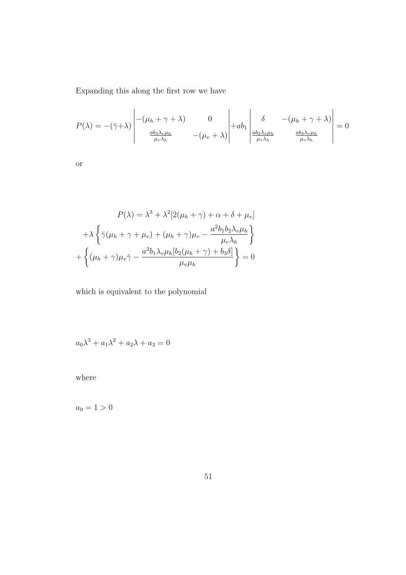
The graphs of population agaist time was plotted. The following numer-

ical values were used: a = 0.01, b1 = 0.2, b2 = b3 = 0.5, δ = 0.005, γ =

0.03, α = 0.01, µv = 0.04, µh = 0.02, λv = 10 and λh = 20 with initial condi-

tions Nh(0) = 520, Nv(0) = 150, Ih(0) = 10, Ah(0) = 0 and Iv(0) = 0 giving

R0 = 0.001058. In the first graph all compartments populations were plotted

against time and it was clear that populations increased with time level-

ing off in the long-run. In the second figure only the disease compartment

populations were considered.

70

71

72

4 CONCLUSION

We modeled malaria as a 5-dimensional system of ordinary differential equa-

tions. We showed the existence and uniqueness of a domain where the model

is epidemiologically and mathematically well-posed. The model was analysed

for the disease free equilibrium and endemic equilibrium. We defined the re-

production number in terms of the parameters. It was also established that

for the basic reproduction number, R0 ≤ 1, the disease free equilibrium point

is asymptotically stable so that the disease dies out after some period of time

and if R0 > 0, the disease free equilibrium is unstable. We also established

that when R0 > 1 then the endemic equilibrium is locally asymptotically

stable, and unstable if R0 < 1. From the numerical simulations it is clear

that populations increase with time and finally leveling off in the long run

when carrying capacity is reached.

73

References

[1] Nadjm B, Behrens RH (2012). ”Malaria: An update for physi-

cians”. Infectious Disease Clinics of North America 26 (2): 24359.

doi:10.1016/j.idc.2012.03.010. PMID 22632637.

[2] World Malaria Report (2012). World Health Organization.

[3] Olupot-Olupot P, Maitland, K (2013). ”Management of severe

malaria: Results from recent trials”. Advances in Experimental

Medicine and Biology. Advances in Experimental Medicine and Biology

764: 24150. doi:10.1007/978-1-4614-4726-9-20. ISBN 978-1-4614-4725-

2. PMID 23654072.

[4] Murray CJ, Rosenfeld LC, Lim SS, Andrews KG, Foreman KJ, Har-

ing D, Fullman N, Naghavi M, Lozano R, Lopez AD (2012). ”Global

malaria mortality between 1980 and 2010: A systematic analysis”.

Lancet 379 (9814): 41331. doi:10.1016/S0140-6736(12)60034-8. PMID

22305225.

[5] Lozano R, et al. (2012). ”Global and regional mortality from 235 causes

of death for 20 age groups in 1990 and 2010: A systematic analysis for

the Global Burden of Disease Study 2010”. Lancet 380 (9859): 2095128.

doi:10.1016/S0140-6736(12)61728-0. PMID 23245604.

[6] Hartman TK, Rogerson SJ, Fischer PR (2010). ”The impact of ma-

ternal malaria on newborns”. Annals of Tropical Paediatrics 30 (4):

74

27182. doi:10.1179/146532810X12858955921032. PMID 21118620.

[7] Taylor WR, Hanson J, Turner GD, White NJ, Dondorp AM (2012).

”Respiratory manifestations of malaria”. Chest 142 (2): 492505.

doi:10.1378/chest.11-2655. PMID 22871759.

[8] Kajfasz P (2009). ”Malaria prevention”. International Maritime Health

60 (12): 6770. PMID 20205131.

[9] Howitt P, Darzi A, Yang GZ, Ashrafian H, Atun R, Barlow J, Blake-

more A, Bull AM, Car J, Conteh L, Cooke GS, Ford N, Gregson SA,

Kerr K, King D, Kulendran M, Malkin RA, Majeed A, Matlin S, Mer-

rifield R, Penfold HA, Reid SD, Smith PC, Stevens MM, Templeton

MR, Vincent C, Wilson E (2012). ”Technologies for global health”. The

Lancet 380 (9840): 50735. doi:10.1016/S0140-6736(12)61127-1. PMID

22857974.

[10] Layne SP. ”Principles of Infectious Disease Epidemiology” (PDF). EPI

220. UCLA Department of Epidemiology. Archived from the original

on 2006-02-20. Retrieved 2007-06-15.

[11] Provost C (April 25, 2011). ”World Malaria Day: Which countries are

the hardest hit? Get the full data”. The Guardian. Retrieved 2012-05-

03.

[12] Guerra CA, Hay SI, Lucioparedes LS, Gikandi PW, Tatem AJ, Noor

AM, Snow RW (2007). ”Assembling a global database of malaria par-

75

asite prevalence for the Malaria Atlas Project”. Malaria Journal 6 (6):

17. doi:10.1186/1475-2875-6-17. PMC 1805762. PMID 17306022.

[13] Hay SI, Okiro EA, Gething PW, Patil AP, Tatem AJ, Guerra CA,

Snow RW (2010). ”Estimating the global clinical burden of Plasmod-

ium falciparum malaria in 2007”. In Mueller, Ivo. PLoS Medicine

7 (6): e1000290. doi:10.1371/journal.pmed.1000290. PMC 2885984.

PMID 20563310.

[14] Feachem RG, Phillips AA, Hwang J, Cotter C, Wielgosz B, Greenwood

BM, Sabot O, Rodriguez MH, Abeyasinghe RR, Ghebreyesus TA, Snow

RW (2010). ”Shrinking the malaria map: progress and prospects”.

Lancet 376 (9752): 156678. doi:10.1016/S0140-6736(10)61270-6. PMC

3044848. PMID 21035842.

[15] Greenwood B, Mutabingwa T (2002). ”Malaria in 2002”. Nature 415

(6872): 6702. doi:10.1038/415670a. PMID 11832954.

[16] Jamieson A, Toovey S, Maurel M (2006). Malaria: A Traveller’s Guide.

Struik. p. 30. ISBN 978-1-77007-353-1.

[17] Abeku TA (2007). ”Response to malaria epidemics in Africa”. Emerg-

ing Infectious Diseases 14 (5): 6816. doi:10.3201/eid1305.061333. PMC

2738452. PMID 17553244.

[18] Cui L, Yan G, Sattabongkot J, Cao Y, Chen B, Chen X, Fan Q, Fang Q,

Jongwutiwes S, Parker D, Sirichaisinthop J, Kyaw MP, Su XZ, Yang H,

76

Yang Z, Wang B, Xu J, Zheng B, Zhong D, Zhou G (2012). ”Malaria in

the Greater Mekong Subregion: Heterogeneity and complexity”. Acta

Tropica 121 (3): 22739.

[19] Machault V, Vignolles C, Borchi F, Vounatsou P, Pages F, Briolant S,

Lacaux JP, Rogier C (2011). ”The use of remotely sensed environmental

data in the study of malaria” (PDF). Geospatial Health 5 (2): 15168.

PMID 21590665.

[20] Gething PW, Patil AP, Smith DL, Guerra CA, Elyazar IR, Johnston

GL, Tatem AJ, Hay SI (2011). ”A new world malaria map: Plas-

modium falciparum endemicity in 2010”. Malaria Journal 10 (1): 378.

doi:10.1186/1475-2875-10-378. PMC 3274487. PMID 22185615.

[21] Mueller I, Zimmerman PA, Reeder JC (2007). ”Plasmodium malariae

and Plasmodium ovalethe ”bashful” malaria parasites”. Trends in Par-

asitology 23 (6): 27883. doi:10.1016/j.pt.2007.04.009. PMC 3728836.

PMID 17459775.

[22] Collins WE (2012). ”Plasmodium knowlesi: A malaria parasite of

monkeys and humans”. Annual Review of Entomology 57: 10721.

doi:10.1146/annurev-ento-121510-133540. PMID 22149265.

[23] Schlagenhauf-Lawlor 2008, pp. 701.

[24] Cowman AF, Berry D, Baum J (2012). ”The cellular and molecular

basis for malaria parasite invasion of the human red blood cell”. Jour-

77

nal of Cell Biology 198 (6): 96171. doi:10.1083/jcb.201206112. PMC

3444787. PMID 22986493.

[25] Arrow KJ, Panosian C, Gelband H, Institute of Medicine (U.S.). Com-

mittee on the Economics of Antimalarial Drugs (2004). Saving Lives,

Buying Time: Economics of Malaria Drugs in an Age of Resistance.

National Academies Press. p. 141. ISBN 978-0-309-09218-0.

[26] Owusu-Ofori AK, Parry C, Bates I (2010). ”Transfusion-transmitted

malaria in countries where malaria is endemic: A review of the liter-

ature from sub-Saharan Africa”. Clinical Infectious Diseases 51 (10):

11928. doi:10.1086/656806. PMID 20929356.

[27] Fairhurst RM, Wellems TE (2010). ”Chapter 275. Plasmodium species

(malaria)”. In Mandell GL, Bennett JE, Dolin R (eds). Mandell, Dou-

glas, and Bennett’s Principles and Practice of Infectious Diseases 2

(7th ed.). Philadelphia, Pennsylvania: Churchill Livingstone/Elsevier.

pp. 34373462. ISBN 978-0-443-06839-3.

[28] Bartoloni A, Zammarchi L (2012). ”Clinical aspects of uncomplicated

and severe malaria”. Mediterranean Journal of Hematology and In-

fectious Diseases 4 (1): e2012026. doi:10.4084/MJHID.2012.026. PMC

3375727. PMID 22708041.

[29] Beare NA, Taylor TE, Harding SP, Lewallen S, Molyneux ME (2006).

”Malarial retinopathy: A newly established diagnostic sign in severe

78

malaria”. American Journal of Tropical Medicine and Hygiene 75 (5):

7907. PMC 2367432. PMID 17123967.

[30] Ferri FF (2009). ”Chapter 332. Protozoal infections”. Ferri’s Color At-

las and Text of Clinical Medicine. Elsevier Health Sciences. p. 1159.

ISBN 978-1-4160-4919-7.

[31] Anderson RM, May RM: Infectious diseases of humans: dynamics and

control. London: Oxford University Press; 1991.

[32] The malERA Consultative Group on Modeling: A Research agenda for

malaria eradication: modeling. PLoS Med 2011, 8:e1000403.

[33] Roll Back Malaria Partnership: The global malaria action plan, for a

malaria free world . Geneva, Switzerland; 2008.

[34] Alonso PL, Brown G, Arevalo M, Binka F, Chitnis C, Collins F,

Doumbo O, Greenwood B, Hall L, Levine M, Mendis K, Newmann R,

Plowe C, Rodriguez MH, Sinden R, Slusker L, Tanner M: A research

agenda to underpin malaria eradication. PLoS Med 2011, 8: e1000406.

[35] Harper K, Armelagos G (2011). ”The changing disease-scape

in the third epidemiological transition”. International Journal

of Environmental Research and Public Health 7 (2): 67597.

doi:10.3390/ijerph7020675. PMC 2872288. PMID 20616997.

[36] Prugnolle F, Durand P, Ollomo B, Duval L, Ariey F, Arnathau

C, Gonzalez JP, Leroy E, Renaud F (2011). ”A fresh look at

79

the origin of Plasmodium falciparum, the most malignant malaria

agent”. In Manchester, Marianne. PLoS Pathogens 7 (2): e1001283.

doi:10.1371/journal.ppat.1001283. PMC 3044689. PMID 21383971.

[37] Cox F (2002). ”History of human parasitology”. Clinical Microbiology

Reviews 15 (4): 595612. doi:10.1128/CMR.15.4.595-612.2002. PMC

126866. PMID 12364371.

[38] ”DNA clues to malaria in ancient Rome”. BBC News. February 20,

2001., in reference to Sallares R, Gomzi S (2001). ”Biomolecular ar-

chaeology of malaria”. Ancient Biomolecules 3 (3): 195213. OCLC

538284457.

[39] Sallares R (2002). Malaria and Rome: A History

of Malaria in Ancient Italy. Oxford University Press.

doi:10.1093/acprof:oso/9780199248506.001.0001. ISBN 978-0-19-

924850-6.

[40] Hays JN (2005). Epidemics and Pandemics: Their Impacts on Human

History. Santa Barbara, California: ABC-CLIO. p. 11. ISBN 978-1-

85109-658-9.

[41] Reiter P (2000). ”From Shakespeare to Defoe: Malaria in England

in the Little Ice Age”. Emerging Infectious Diseases 6 (1): 111.

doi:10.3201/eid0601.000101. PMC 2627969. PMID 10653562.

[42] Lindemann M (1999). Medicine and Society in Early Modern Europe.

80

Cambridge University Press. p. 62. ISBN 978-0-521-42354-0.

[43] Gratz NG, World Health Organization (2006). The Vector- and

Rodent-borne Diseases of Europe and North America: Their Distri-

bution and Public Health Burden. Cambridge University Press. p. 33.

ISBN 978-0-521-85447-4.

[44] Webb Jr JLA (2009). Humanity’s Burden: A Global History of Malaria.

Cambridge University Press. ISBN 978-0-521-67012-8.

[45] Bray RS (2004). Armies of Pestilence: The Effects of Pandemics on

History. James Clarke. p. 102. ISBN 978-0-227-17240-7.

[46] Byrne JP (2008). Encyclopedia of Pestilence, Pandemics, and Plagues:

A-M. ABC-CLIO. p. 383. ISBN 978-0-313-34102-1.

[47] ”The Nobel Prize in Physiology or Medicine 1907: Alphonse Laveran”.

The Nobel Foundation. Retrieved 2012-05-14.

[48] Tan SY, Sung H (2008). ”Carlos Juan Finlay (18331915): Of

mosquitoes and yellow fever” (PDF). Singapore Medical Journal 49

(5): 3701. PMID 18465043.

[49] Chernin E (1983). ”Josiah Clark Nott, insects, and yellow fever”. Bul-

letin of the New York Academy of Medicine 59 (9): 790802. PMC

1911699. PMID 6140039.

[50] Chernin E (1977). ”Patrick Manson (18441922) and the transmission

81

of filariasis”. American Journal of Tropical Medicine and Hygiene 26

(5 Pt 2 Suppl): 106570. PMID 20786.

[51] ”The Nobel Prize in Physiology or Medicine 1902: Ronald Ross”. The

Nobel Foundation. Retrieved 2012-05-14.

[52] ”Ross and the Discovery that Mosquitoes Transmit Malaria Parasites”.

CDC Malaria website. Archived from the original on 2007-06-02. Re-

trieved 2012-06-14.

[53] Simmons JS (1979). Malaria in Panama. Ayer Publishing. ISBN 978-

0-405-10628-6.

[54] Kaufman TS, Rveda EA (2005). ”The quest for quinine: Those

who won the battles and those who won the war”. Ange-

wandte Chemie (International Edition in English) 44 (6): 85485.

doi:10.1002/anie.200400663. PMID 15669029.

[55] Pelletier PJ, Caventou JB (1820). ”Des recherches chimiques sur les

Quinquinas” [Chemical research on quinquinas]. Annales de Chimie et

de Physique (in French) 15: 33765.

[56] Kyle R, Shampe M (1974). ”Discoverers of quinine”. Jour-

nal of the American Medical Association 229 (4): 462.

doi:10.1001/jama.229.4.462. PMID 4600403.

[57] Achan J, Talisuna AO, Erhart A, Yeka A, Tibenderana JK, Bali-

raine FN, Rosenthal PJ, D’Alessandro U (2011). ”Quinine, an old

82

anti-malarial drug in a modern world: Role in the treatment of

malaria”. Malaria Journal 10 (1): 144. doi:10.1186/1475-2875-10-144.

PMC 3121651. PMID 21609473.

[58] Hsu E (2006). ”Reflections on the ’discovery’ of the antimalarial

qinghao”. British Journal of Clinical Pharmacology 61 (3): 66670.

doi:10.1111/j.1365-2125.2006.02673.x. PMC 1885105. PMID 16722826.

open access publication - free to read

[59] Vogel V (2013). ”Malaria as a Lifesaving Therapy”. Science 342 (6159):

684687. doi:10.1126/science.342.6159.684.

[60] ”Eradication of Malaria in the United States (19471951)”. US Centers

for Disease Control and Prevention. February 8, 2010. Retrieved 2012-

05-02.

[61] van den Berg H (2009). ”Global status of DDT and its alternatives for

use in vector control to prevent disease”. Environmental Health Per-

spectives 117 (11): 165663. doi:10.1289/ehp.0900785. PMC 2801202.

PMID 20049114.

[62] Killeen G, Fillinger U, Kiche I, Gouagna L, Knols B (2002). ”Eradica-

tion of Anopheles gambiae from Brazil: Lessons for malaria control in

Africa?”. Lancet Infectious Diseases 2 (10): 61827. doi:10.1016/S1473-

3099(02)00397-3. PMID 12383612.

[63] Vanderberg JP (2009). ”Reflections on early malaria vaccine studies,

83

the first successful human malaria vaccination, and beyond”. Vaccine

27 (1): 29. doi:10.1016/j.vaccine.2008.10.028. PMC 2637529. PMID

18973784.

[64] Ross SR. 1908 Report on the prevention of malaria in Mauritius. Lon-

don, UK: Waterlow and Sons Limited.

[65] Ross SR. 1911 The prevention of malaria. New York, NY: Dutton.

[66] Macdonald G. 1956 Epidemiological basis of malaria control. Bull.

World Health Organ. 15, 613626.

[67] Macdonald G. 1956 Theory of the eradication of malaria. Bull. World

Health Organ. 15, 369387.

[68] Macdonald G,Gckel GW. 1964 The malaria parasite rate and interrup-

tion of transmission. Bull. World Health Organ. 31, 365377.

[69] WHO. 1957 Expert Committee on Malaria, sixth report. Technical

Report Series 123, World Health Organization, Geneva.

[70] Macdonald G. 1957 The epidemiology and control of malaria. Oxford,

UK: Oxford University Press.

[71] On the use of mathematical models of malaria transmission. Koella JC

Acta Trop. 1991 Apr; 49(1):1-25..

[72] Yang HM. Malaria transmission model for different levels of acquired

immunity and temperature-dependent parameters (vector) Revista de

84

Sade Pblica. 2000;34:223231.

[73] Macdonald G, Cuellar CB, Foll CV. 1968 The dynamics of malaria.

Bull. World Health Organ. 38, 743.

[74] Smith DL, Battle KE, Hay SI, Barker CM, Scott TW, McKenzie

FE. 2012 Ross, macdonald and a theory for the dynamics and con-

trol of mosquito-transmitted pathogens. PLoS Pathogens 8, e1002588.

doi:10.1371/journal.ppat.1002588 (doi:10.1371/journal.ppat.1002588).

[75] John CC, Riedesel MA, Magak NG, Lindblade KA, Menge DM, Hodges

JS, Vulule JM, Akhwale W: Possible interruption of malaria transmis-

sion, highland Kenya, 20072008. Infect Dis 2009, 15:1917-1924.

[76] Fernando SD, Abeyasinghe RR, Galappaththy GN, Rajapaksa LC: Ab-

sence of asymptomatic malaria infections in previously high endemic

areas of Sri Lanka. Am J Trop Med Hyg 2009, 81:763-767.

[77] P Van Den Driessche and J. Watmough,”Reproduction numbers and

subthreshold Endemic Equilibria for Compartmental models of Disease

tansmission,” Mathematical Biosciences, Vol. 180, No.1-2,2002, PP.29-

48.

[78] R.M. Anderson, R.M.May, Infectious Diseases of humans: Dynamics

and control, Oxford Univeresity press, Oxford, 1991, PP.451-524.

[79] Bony and J. Michael, vol.19, No.1, 1969, PP. 277-304.

85

[80] M. Quincampoix, ”Differential inclusions and Target problems,” SIAM

Journal on control and optimization, Vol. 30, NO.2,1992, PP 324-335.

[81] M.Vidyasagar,”Decomposition techniques for largescale systems with

non-additive interactions: stability and stabilizability,” IEE Transac-

tions on Automatic control, Vol.25, NO. 4, 1980,PP.773-779.

[82] N. Chitnis. Using mathematical models in controlling the spread of

malaria. PhD thesis, University of Arizona, 2005.

[83] Filipe JAN, Riley EM, Darkeley CJ, Sutherland CJ, Ghani AC. De-

termination of the processes driving the acquisition of immunity to

malaria using a mathematical transmission model. PLoS Comp Biol.

2007;3:25692579.

[84] N. Chitnis, J.M. Cushing, and M. Hyman. Determining important pa-

rameters in the spread of malaria through the sensitivity analysis of a

mathematical model. Bulletin of mathematical Biology,70:1272-1296,

2008.

[85] A.Ngwa and W.S.shu. A mathematical model for endemic malaria with

variable human and mosquito populations. Math. Comput. Mathemat-

ical modeling, 32:747-763, 2000.

[86] Anderson RM, May RM. Infectious diseases of humans: dynamics and

control. London: Oxford University Press; 1991

86

[87] H.W. Hethcote , ”Qualitative analysis of communicable Disease mod-

els,” Mathematical Biosciences, Vol.28,No. 3-4, 1976, pp. 335-356.

[88] Mabunda S, Aponte JJ, Tiago A, Alonso P. A country-wide malaria

survey in Mozambique. II. Malaria attributable proportion of fever and

establishment of malaria case definition in children across different epi-

demiological settings. Malar J. 2009;8:74. doi: 10.1186/1475-2875-8-74.

[89] Surez-Mutis MC, Cuervo P, Leoratti FM, Moraes-Avila SL, Ferreira

AW, Fernandes O, Coura JR: Cross sectional study reveals a high per-

centage of asymptomatic Plasmodium vivax infection in the Amazon

Rio Negro area, Brazil. Rev Inst Med Trop Sao Paulo 2007, 49:159-164.

[90] Cucunub ZM, Guerra AP, Rahirant SJ, Rivera JA, Corts LJ, Nicholls

RS: Asymptomatic Plasmodium spp. infection in Tierralta, Colombia.

Mem Inst Oswaldo Cruz 2008, 103:668-673.

[91] Harris I, Sharrock WW, Bain LM, Gray KA, Bobogare A, Boaz L,

Lilley K, Krause D, Vallely A, Johnson ML, Gatton ML, Shanks GD,

Cheng Q: A large proportion of asymptomatic Plasmodium infections

with low and sub-microscopic parasite densities in the low transmission

setting of Temotu Province, Solomon Islands: challenges for malaria

diagnostics in an elimination setting. Malar J 2010, 9:254.

[92] Lee PW, Liu CT, Rampao HS, do Rosario VE, Shaio MF: Pre-

elimination of malaria on the island of Prncipe. Malar J 2010, 9:26.

87

[93] Staalsoe T, Hviid L: The role of variant-specific immunity in asymp-

tomatic malaria infections: maintaining a fine balance. Parasitol Today

1998, 14:177-178.

[94] Bousema JT, Gouagna LC, Drakeley CJ, Meutstege AM, Okech BA,

Akim IN, Beier JC, Githure JI, Sauerwein RW: Plasmodium falciparum

gametocyte carriage in asymptomatic children in western Kenya. Malar

J 2004, 3:18.

[95] Crookston BT, Alder SC, Boakye I, Merrill RM, Amuasi JH, Porucznik

CA, Stanford JB, Dickerson TT, Dearden KA, Hale DC, Sylverken J,

Snow BS, Osei-Akoto A, Ansong D: Exploring the relationship be-

tween chronic undernutrition and asymptomatic malaria in Ghanaian

children. Malar J 2010, 9:39.

[96] Owusu-Agyei S, Koram KA, Baird JK, Utz GC, Binka FN, Nkrumah

FK, Fryauff DJ, Hoffman SL: Incidence of symptomatic and asymp-

tomatic Plasmodium falciparum infection following curative therapy in

adult residents of Northern Ghana. Am J Trop Med Hyg 2001, 65:197-

203.

[97] Males S, Gaye O, Garcia A: Long-term asymptomatic carriage of Plas-

modium falciparum protects from malaria attacks: a prospective study

among SeneGhalese children. Clin Infect Dis 2008, 46:516-522.

[98] Le Port A, Cot M, Etard JF, Gaye O, Migot-Nabias F, Garcia A:

88

Relation between Plasmodium falciparum asymptomatic infection and

malaria attacks in a cohort of SeneGhalese children. Malar J 2008,

7:193.

[99] Klein Klouwenberg PM, Oyakhirome S, Schwarz NG, Glser B, Issifou

S, Kiessling G, Klpfer A, Kremsner PG, Lngin M, Lassmann B, Necek

M, Ptschke M, Ritz A, Grobusch MP: Malaria and asymptomatic par-

asitaemia in Gabonese infants under the age of 3months. Acta Trop

2005, 95:81-85.

[100] Nkoghe D, Akue JP, Gonzalez JP, Leroy EM: Prevalence of Plasmod-

ium falciparum infection in asymptomatic rural Gabonese populations.

Malar J 2011, 10:33.

[101] Eke RA, Chigbu LN, Nwachukwu W: High prevalence of asymptomatic

Plasmodium infection in a suburb of Aba Town, Nigeria. Ann of Afr

Med 2006, 5:42-45.

[102] Achidi EA, Perlmann H, Berzins K: Asymptomatic malaria para-

sitaemia and seroreactivities to Plasmodium falciparum antigens in

blood donors from Ibadan, south-western Nigeria. Ann Trop Med Par-

asitol 1995, 89:601-610.

[103] Njama-Meya D, Kamya MR, Dorsey G: Asymptomatic parasitaemia as

a risk factor for symptomatic malaria in a cohort of Ugandan children.

Trop Med Int Health 2004, 9:862-868.

89

[104] Coleman RE, Maneechai N, Rachaphaew N, Kumpitak C, Miller RS,

Soyseng V, Thimasarn K, Sattabongkot J: Comparison of field and

expert laboratory microscopy for active surveillance for asymptomatic

Plasmodium falciparum and Plasmodium vivax in western Thailand.

Am J Trop Med Hyg 2002, 67:141-144.

[105] Richards AK, Smith L, Mullany LC, Lee CI, Whichard E, Banek K,

Mahn M, ShweOo EK, Lee TJ: Prevalence of Plasmodium falciparum

in active conflict areas of eastern Burma: a summary of cross-sectional

data. Confl Health 2007, 1:9.

[106] Bin Mohanna MA, Bin Ghouth AS, Rajaa YA: Malaria signs and infec-

tion rate among asymptomatic schoolchildren in Hajr Valley, Yemen.

East Mediterr Health J 2007, 13:35-40.

[107] Roper MH, Torres RS, Goicochea CG, Andersen EM, Guarda JS,

Calampa C, Hightower AW, Magill AJ: The epidemiology of malaria in

an epidemic area of the Peruvian Amazon. Am J Trop Med Hyg 2000,

62:247-256.

[108] Alves FP, Durlacher RR, Menezes MJ, Krieger H, Silva LH, Camargo

EP: High prevalence of asymptomatic Plasmodium vivax and Plasmod-

ium falciparum infections in native Amazonian populations. Am J Trop

Med Hyg 2002, 66:641-648.

[109] Roshanravan B, Kari E, Gilman RH, Cabrera L, Lee E, Metcalfe J,

90

Calderon M, Lescano AG, Montenegro SH, Calampa C, Vinetz JM:

Endemic malaria in the Peruvian Amazon region of Iquitos. Am J Trop

Med Hyg 2003, 69:45-52.

[110] Marcano TJ, Morgado A, Tosta CE, Coura JR: Cross-sectional study

defines difference in malaria morbidity in two Yanomami communi-

ties on Amazonian boundary between Brazil and Venezuela. Mem Inst

Oswaldo Cruz 2004, 99:369-376.

[111] Branch O, Casapia WM, Gamboa DV, Hernandez JN, Alava FF, Ron-

cal N, Alvarez E, Perez EJ, Gotuzzo E: Clustered local transmission and

asymptomatic Plasmodium falciparum and Plasmodium vivax malaria

infections in a recently emerged, hypoendemic Peruvian Amazon com-

munity. Malar J 2005, 4:27.

[112] Cerutti C, Boulos M, Coutinho AF, HatabMdo C, Falqueto A, Rezende

HR, Duarte AM, Collins W, Malafronte RS: Epidemiologic aspects of

the malaria transmission cycle in an area of very low incidence in Brazil.

Malar J 2007, 6:33.

[113] Fugikaha E, Fornazari PA, Penhalbel Rde S, Lorenzetti A, Maroso RD,

Amoras JT, Saraiva AS, Silva RU, Bonini-Domingos CR, Mattos LC,

Rossit AR, Cavasini CE, Machado RL: Molecular screening of Plas-

modium spp. asymptomatic carriers among transfusion centers from

Brazilian Amazon region. Rev Inst Med Trop Sao Paulo 2007, 49:1-4.

91

[114] Gil LH, Tada MS, Katsuragawa TH, Ribolla PE, da Silva LH: Ur-

ban and suburban malaria in Rondnia (Brazilian Western Amazon) II.

Perennial transmissions with high anopheline densities are associated

with human environmental changes. Mem Inst Oswaldo Cruz 2007,

102:271-276.

92