Embed Size (px)
Citation preview

1
Submission for the 2013 IAOS Prize for Young Statisticians
Using kernel methods to
visualise crime data
Dr. Kieran Martin and Dr. Martin Ralphs
Office for National Statistics, UK

2
Abstract
Kernel smoothing methods can be used to better visualise data that are available over
geography. The visualisations creased by these methods allow users to observe trends in the
data which may not be apparent from numerical summaries or point data.
Crime data in the UK has recently been made available to the public at post code level, with
visualisations of the amount of recorded events at each postcode for a given area available
online. In this paper we apply existing kernel smoothing methods to this data, to assess the
use of kernel smoothing methods as applied to open access data.
Kernel smoothing methods are applied to crime data from the greater London metropolitan
area, using methods freely available in R. We also investigate the utility of using simple
methods to smooth the data over time.
The kernel smoothers used are demonstrated to provide effective and useful visualisations of
the data, and it is proposed that these methods should be more widely applied in data
visualisations in the future.

3
1. Introduction
With the increasing level of access to data, users have an unprecedented access to statistics
produced across government. There are currently over 8000 data sets available at data.gov.uk.
This increased access presents issues with confidentiality; releasing such data should not
compromise the identity for individuals or businesses from which statistics are gathered. This
issue has been discussed in a government white paper, Unleashing the Potential (2012). The
government wishes to provide more transparent data, but avoid compromising people’s
identity. Large data releases are also likely to contain mistakes (see Hand, 2012). Approaches
to releasing administrative data thus far tend to have focused on releasing data assigned to a
specific location, often released in a less disclosive form by attaching multiple records to one
geographical location.
Raw point estimates can be difficult to understand, especially when they are given over time
or space. Simple data summaries (means over an area) can improve comprehension, but
doing so can remove some of the spatial patterns that were of interest initially, as well as
privilege particular geographical boundaries. One method of summarising data over
geography which avoids this problem is to “smooth” the data, creating summaries over small
geographical areas which blend together naturally. There have been some investigations into
this by the Office for National Statistics (ONS); Carrington et al (2007), produced smoothed
estimates for mortality where estimates were smoothed by simple averages, and more
recently Ralphs (2011) applied kernel smoothing methods to business data.
Kernel density estimation is a so called “non-parametric” method for summarising data
gathered over one or more dimensions. It can be used in multiple contexts, such as estimating
the shape of a density function, or looking for underlying trends in data. Kernel density
estimation is a descriptive measure, applying to observed data, and does not necessarily
provide accurate predictions for future data as parametric methods can.
One use of kernel density estimation can be to visualise patterns in spatial data, such as levels
of unemployment or poverty across the country. In this report we illustrate the use of kernel
smoothing methods by application to a publically available data set. Smoothed data will
naturally reduce how easy it is to identify individuals, and help control against mistakes in
releases by averaging out errors.
The British police keep a record of all reported crime in each constabulary. This is one
method used in the United Kingdom for recording crime levels; the British Crime Survey is
also used to supplement recorded crime by surveying people’s experience of crime in the last
12 months.
For the last two years police.uk has released monthly information on the number of criminal
events that have been recorded in police authorities in England and Wales. This release
combines all crimes recorded across that month, and the events are then associated with the
centre of the postcode in which said crime was reported to have occurred. While this is a
useful visualisation at a local level, as of yet there is no real summary of crime statistics
across an area, meaning like with like comparisons are difficult. Comparing one month with

4
another in a particular area can only be done by examining the raw totals of crimes recorded
for an area.
This paper describes the application of kernel smoothing methods to crime data. In section 2
the general theory of the kernel density methods used are briefly described, and how the
methods were applied to the crime data is outlined in section 3. Section 4 presents results for
crime across the greater London metropolitan area for several crime types, as well as for a
smaller area, in Camden. Section 5 presents results when the crime data has been averaged
over time, to try to dampen the effect of small spikes in crime in a particular month. Section 6
details conclusions and proposals for further investigation.
2. Kernel density estimation for spatial point process patterns
Kernel density estimation involves applying a function (known as a “kernel”) to each data
point, which averages the location of that point with respect to the location of other data
points. The method has been extended to multiple dimensions and provides an effective
method for estimating geographical density. There is a good deal of literature discussing
kernel density estimation, such as Simonoff, (1996); kernel density estimation was applied in
this paper using the package spatstat in R (for more details, see Baddeley and Turner 2005).
Figure 1 provides an illustration of how this works in practice. The figure shows a number of
data points scattered across a two dimensional space. In kernel density estimation, a smooth,
curved surface in the form of a kernel function (which looks a little like a tent in the diagram)
is placed at each data point. The value of the kernel function is highest at the location of the
point, and diminishes with increasing distance from the point.
Figure 1: visualisation of kernel smoothing process
Now follows a brief introduction to the mathematical underpinnings of kernel estimation.
Given a data set (x1,...,xn)T where xi=(xi1,...,xid)
T, d being the dimension being averaged over.
Kernel density estimation uses a pre-defined kernel, K, and a bandwidth matrix H to produce
an estimate of the density of said data. The estimate of the density of the data at a point x is
then:
�n
i
i=1
1F ( )= ( - ),
n∑ H
x K x x
where,
1/ 2 1/ 2( ) | | ( ).− −
=HK x H K H x �
5
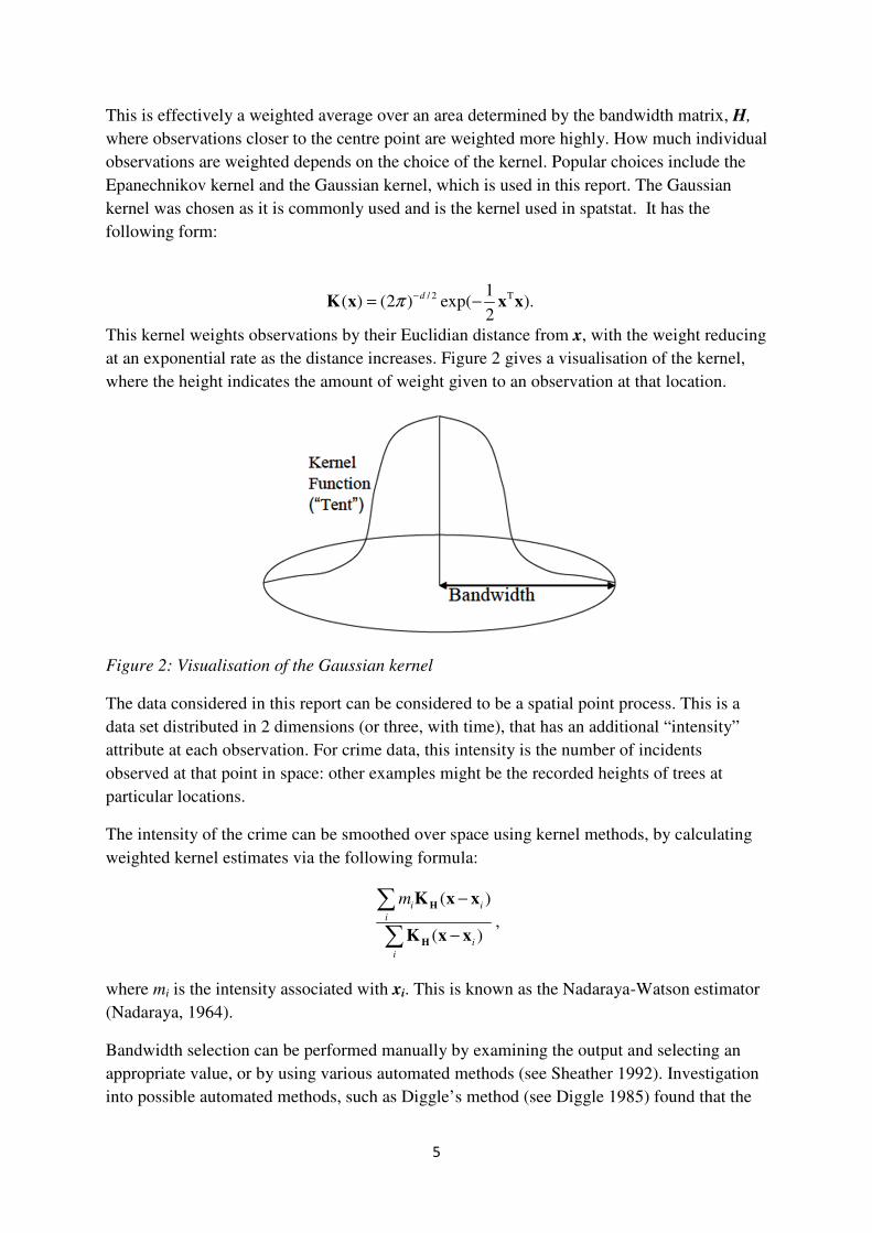
This is effectively a weighted average over an area determined by the bandwidth matrix, H,
where observations closer to the centre point are weighted more highly. How much individual
observations are weighted depends on the choice of the kernel. Popular choices include the
Epanechnikov kernel and the Gaussian kernel, which is used in this report. The Gaussian
kernel was chosen as it is commonly used and is the kernel used in spatstat. It has the
following form:
/ 2 T1( ) (2 ) exp( ).
2
dπ
−
= −K x x x �
This kernel weights observations by their Euclidian distance from x, with the weight reducing
at an exponential rate as the distance increases. Figure 2 gives a visualisation of the kernel,
where the height indicates the amount of weight given to an observation at that location.
Figure 2: Visualisation of the Gaussian kernel
The data considered in this report can be considered to be a spatial point process. This is a
data set distributed in 2 dimensions (or three, with time), that has an additional “intensity”
attribute at each observation. For crime data, this intensity is the number of incidents
observed at that point in space: other examples might be the recorded heights of trees at
particular locations.
The intensity of the crime can be smoothed over space using kernel methods, by calculating
weighted kernel estimates via the following formula:
( )
( )
i i
i
i
i
m −
−
∑
∑
H
H
K x x
K x x,
where mi is the intensity associated with xi. This is known as the Nadaraya-Watson estimator
(Nadaraya, 1964).
Bandwidth selection can be performed manually by examining the output and selecting an
appropriate value, or by using various automated methods (see Sheather 1992). Investigation
into possible automated methods, such as Diggle’s method (see Diggle 1985) found that the
6
bandwidths obtained over smoothed the results at small geographies, and were
computationally difficult to obtain at high geographies. It was found that Scott’s rule of
thumb (Scott 1992, page 152) provided good values for the bandwidth and was easy to
quickly calculate. Scott’s rule has the form:
1/( 4),
d
j jh n σ− +
=
where hj is the bandwidth for the jth dimension, j=1,..,d (d=2 in this paper), n the number of
observations and jσ is the standard deviation of the observations in the jth dimension. This is
a simple method, which is based on providing the optimal bandwidth for a reference
distribution, in this case a multivariate normal distribution.
3. Applying kernel density estimation to crime data
The crime data as released by the home office is given in the form of the number of events
associated with a particular location. While in practice these events will have not occurred in
the exact same geographical location, to avoid disclosure the outputs are given in this form.
This means that the data is treated as a spatial point process, with the number of events being
the intensity, m.
Treating the data as a spatial process implies that each point is an observation of intensity. In
this case, the model needs to take account of the fact that most locations do not observe
crimes in any given month, otherwise the smoothing process will assume that the minimum
value of crimes observed at any location is 1. To account for this, all crime data over the two
year period available was gathered to populate London with possible locations where crimes
might occur and each location was assigned an intensity of 0; then, in any given month, those
locations which recorded crimes had their intensity value replaced with the number of
recorded crimes. Note that there may be some locations that in the two year period that data is
available for did not report any criminal events, and thus are missed by this method, but as
recorded crimes include anti-social behaviour it is hoped that the majority of postcodes are
included by this method.
Two different areas were considered: the greater metropolitan London area, and a small area
which includes south Camden and Euston. This latter area was chosen to demonstrate the
kernel smoothing method applied to smaller geographies.
For each geographical area multiple crime types could be considered. This paper focuses on
vehicle crime, but this method can easily be applied to any crime type. The chosen bandwidth
depends on the total number (and spread) of points smoothed over, so is constant across
crime type, but varies depending on the level of geography considered.

7
4. Kernel smoothing crime over London
Crime maps were generated for each month from 03/2011-08/2011 for vehicle crime. These
are displayed for London in Figure 3. The scale gives the average number of events in that
area.
This figure demonstrates the power of this technique. It can be seen that while there is some
variance in crime levels between different months, the hot spots remain in similar locations.
In particular, vehicle crime remains high in north east London throughout the six month
period considered. Visualisations at any level which include greater than 10,000 crimes are
not currently available at police.uk.
Figure 4 displays the results for vehicle crime in Camden. The figure also includes the
recorded crime events for that month, represented by circles, which are sized proportional to
the number of recorded events at the centre of the circle. This allows a comparison between
currently available crime visualisations and the new method.
Figure 3: Vehicle crime in London between 03/2011 and 08/2011
It is clear that over small areas crime is more variable, which is possibly unsurprising, as
smaller areas will show small changes each month, while across London these minor changes
8
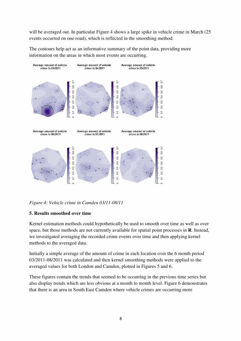
will be averaged out. In particular Figure 4 shows a large spike in vehicle crime in March (25
events occurred on one road), which is reflected in the smoothing method.
The contours help act as an informative summary of the point data, providing more
information on the areas in which most events are occurring.
Figure 4: Vehicle crime in Camden 03/11-08/11
5. Results smoothed over time
Kernel estimation methods could hypothetically be used to smooth over time as well as over
space, but those methods are not currently available for spatial point processes in R. Instead,
we investigated averaging the recorded crime events over time and then applying kernel
methods to the averaged data.
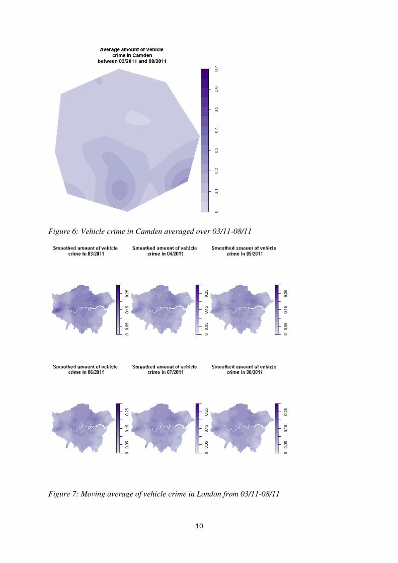
Initially a simple average of the amount of crime in each location over the 6 month period
03/2011-08/2011 was calculated and then kernel smoothing methods were applied to the
averaged values for both London and Camden, plotted in Figures 5 and 6.
These figures contain the trends that seemed to be occurring in the previous time series but
also display trends which are less obvious at a month to month level. Figure 6 demonstrates
that there is an area in South East Camden where vehicle crimes are occurring more

9
frequently; this is less apparent when observing individual months.
Figure 5: Vehicle crime in London averaged over 03/11-08/11
Another possible option for averaging data over time is to use a centralised moving average.
For a given lag (two was used here), a centralised moving average gives the value for each
month as the average of the values recorded for that month, and the two months before and
after (with the number depending on the lag).
The method of centralised moving averages has the advantage of smoothing out individual
spikes in each month, and hopefully makes any underlying trend easier to distinguish.
Different weightings can be applied to each month, and the lag can be varied depending on
the practitioner’s understanding of how long it might take for a trend to appear. One
downside of this method is that, as it requires the months before and after the current one, for
a complete time series the last and first two (depending on the size of the lag) observations
will not be using all data, and should not be displayed. In this report we have chosen a subset
of the available data so this does not affect the plots we display, but it is a practical
consideration that should be kept in mind when this technique is applied.
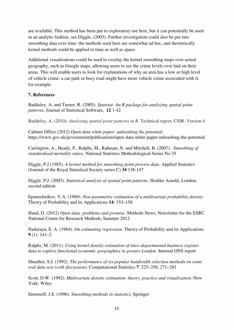
Figures 7-8 display the centralised moving averaged crime data, smoothed over London and
Camden.
Figure 7 shows less month to month variation, while allowing for gradual change, and is
possibly a better visualisation of crime data than Figures 5 and 3 for appreciating the trends
over time of crime in London. The figure is a compromise between simply averaging over the
six months and not averaging at all. The 6 month average removes any short term trends in
the data, while the simple month by month summary can be too sensitive to mild variation.
10
Figure 6: Vehicle crime in Camden averaged over 03/11-08/11
Figure 7: Moving average of vehicle crime in London from 03/11-08/11

11
The downside of this method is that outliers may have too strong an effect. Figure 8, which
displays vehicle crime in Camden, does shows less noise than Figure 4, but picks out a trend
of vehicle crime being concentrated in the south for the first three months which is due to the
extreme spike in vehicle crime in 03/2011 rather than a consistent pattern over that period of
time. The same problem affects Figure 6, which has the same hot spot.
Figure 8: Moving average of vehicle crime in Camden from 03/11-08/11
6. Conclusions and future research
This investigation has demonstrated that kernel smoothing methods can be a powerful tool
for visualising and understanding patterns in crime data. This method could be applied to
additional data sets, such as mortality data and business data; both data sets have had
smoothing techniques applied them in the past. Potentially any data set with a geographical
element could have kernel smoothing methods applied to it.
The method allows users to compare the crime both over time and within an area; this
provides advantages when looking for patterns which may be less apparent in point data. It
also potentially aids in avoiding disclosure issues; if data is released only in smoothed format
then it might be more difficult to identify individuals.
Kernel estimates are relatively easy to calculate in R, which is freely available. Interpreting
patterns and differences between areas can be much more difficult when only point estimates
12
are available. This method has been put to exploratory use here, but it can potentially be used
in an analytic fashion, see Diggle, (2003). Further investigation could also be put into
smoothing data over time: the methods used here are somewhat ad hoc, and theoretically
kernel methods could be applied to time as well as space.
Additional visualisations could be used to overlay the kernel smoothing maps over actual
geography, such as Google maps, allowing users to see the crime levels over laid on their
areas. This will enable users to look for explanations of why an area has a low or high level
of vehicle crime: a car park or busy road might have more vehicle crime associated with it,
for example.
7. References
Baddeley, A. and Turner, R. (2005). Spatstat: An R package for analyzing spatial point
patterns. Journal of Statistical Software, 12 1-42
Baddeley, A. (2010). Analysing spatial point patterns in R. Technical report, CSIR. Version 4
Cabinet Office (2012) Open data white paper: unleashing the potential.
https://www.gov.uk/government/publications/open-data-white-paper-unleashing-the-potential
Carrington, A., Heady, P., Ralphs, M., Rahman, N. and Mitchell, B. (2007). Smoothing of
standardised mortality ratios. National Statistics Methodological Series No 35
Diggle, P.J.(1985). A kernel method for smoothing point process data. Applied Statistics
(Journal of the Royal Statistical Society series C) 34 138-147
Diggle. P.J. (2003). Statistical analysis of spatial point patterns. Hodder Arnold, London,
second edition
Epanechnikov, V.A. (1969). Non-parametric estimation of a multivariate probability density.
Theory of Probability and its Applications 14: 153–158
Hand, D. (2012) Open data: problems and promise. Methods News, Newsletter for the ESRC
National Centre for Research Methods, Summer 2012
Nadaraya, E. A. (1964). On estimating regression. Theory of Probability and its Applications
9 (1): 141–2
Ralphs, M. (2011). Using kernel density estimation of inter-departmental business register
data to explore functional economic geographies in greater London. Internal ONS report
Sheather, S.J. (1992). The performance of six popular bandwidth selection methods on some
real data sets (with discussion). Computational Statistics 7: 225–250, 271–281
Scott, D.W. (1992). Multivariate density estimation. theory, practice and visualization. New
York: Wiley
Simonoff, J.S. (1996). Smoothing methods in statistics. Springer