Embed Size (px)
Citation preview
Using Invariant Theory to Obtain Unknown Size, Shape, Motion, and Three-Dimensional Images from
Single Aperture Synthetic Aperture Radar
October 2005Mark Stuff
This talk contains results which have been contributed to by many persons:
Martin Biancalana (GDAIS)Joseph Gabarino (ALTARUM)Jason Hunt (GDAIS)Susan Wei (GDAIS)Gregory Arnold (AFRL)Vincent Velton (AFRL)Michael Woodroofe (U of Mich)Robert Keener (U of Mich)Pedro Sanchez (Eastern Mich U)
Significant portions of the work reported here were supported by the United States Air Force under contract F33615-02-C-1177
SN-05-0378AFRL/WS Approved
Security and Policy Review Worksheet
Reviewed File:
• ima_presentation_v3.ppt
SN-05-0378: Your document (Presentation/Brief), Using Invariant Theory to Obtain Unknown Size, Shape, Motion, and Three-Dimensional Images from Single Aperture Synthetic Aperture Radar was cleared by AFRL/WS on 11-OCT-05 as Document Number AFRL/WS-05-2360.
2
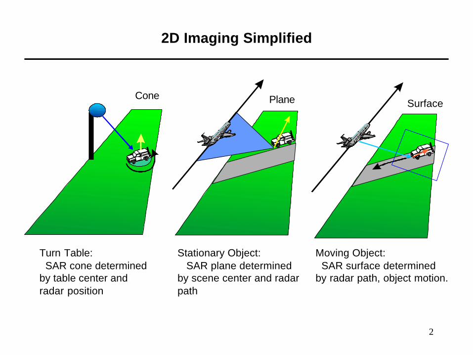
2D Imaging Simplified
Cone Plane Surface
Turn Table:SAR cone determined
by table center and radar position
Stationary Object:SAR plane determined
by scene center and radarpath
Moving Object:SAR surface determined
by radar path, object motion.
3
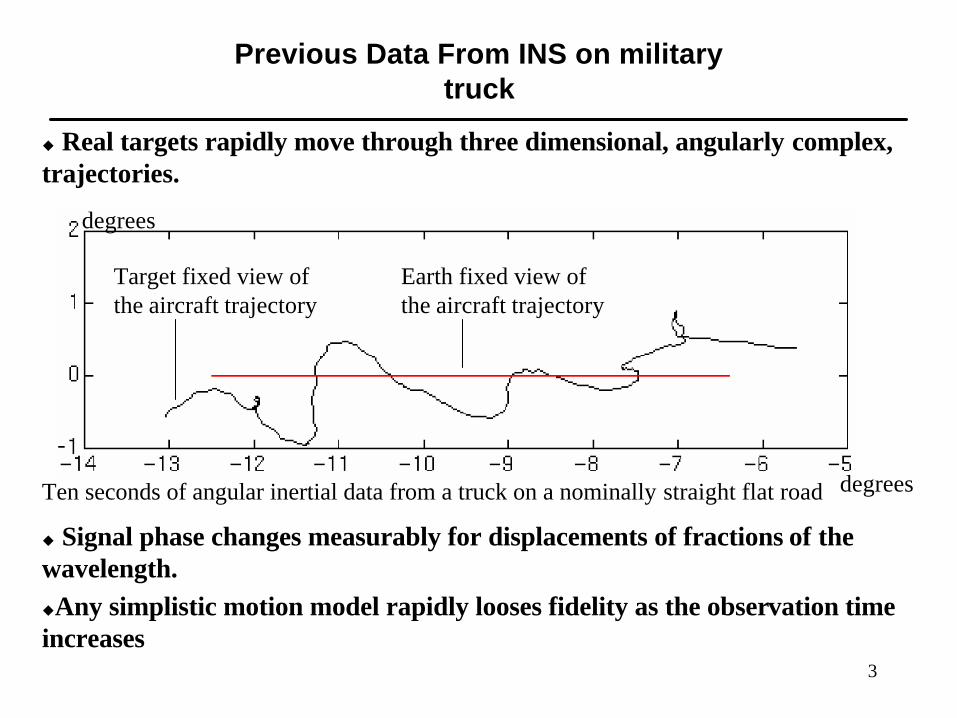
Previous Data From INS on military truck
u Real targets rapidly move through three dimensional, angularly complex, trajectories.
u Signal phase changes measurably for displacements of fractions of the wavelength. uAny simplistic motion model rapidly looses fidelity as the observation time increases
degrees
degrees
Target fixed view of the aircraft trajectory
Earth fixed view of the aircraft trajectory
Ten seconds of angular inertial data from a truck on a nominally straight flat road
4
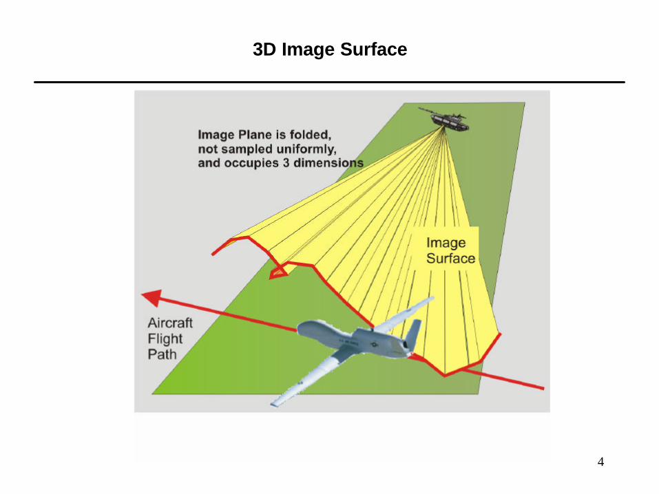
3D Image Surface
5
Implications of complex, random angular motions in three dimensions:
u“Auto-focus” techniques are not enough: uncompensated target rotations limit SAR/ISAR image quality, no matter how well the range translations are compensated.
u Radar data contains three dimensional target size and shape information: No two dimensional image can contain all the target information present in the radar data.
u Sensor flight geometry does not determine viewing geometry: side views are as common as top views; mixed up, mangled, some of each views are what you really get.
u Finite parametric models for the motion rapidly loose fidelity: who can predict the bumps on the road, or the jitters of the driver?

6
Hope for a New Way to Understand Radar Signals
u Moving targets overload conventional processors with information
• System design often ignores or destroys much of this information• Result is smeared, offset images, in 2 dimensions
u The 3DMAGI system exploits the additional information• No restricting assumptions on the complexity of the motions• No prior knowledge of the target type needed; build models on the fly, track objects
which have never been seen before• Developed to work with single aperture systems; extends to multi-aperture systems• Requires understanding of geometric theory and unconventional signal processing
uMost of the work remains to be done: Progress has been made by adapting the work to perceived immediate needs
• Focus moving targets• Track moving targets
7
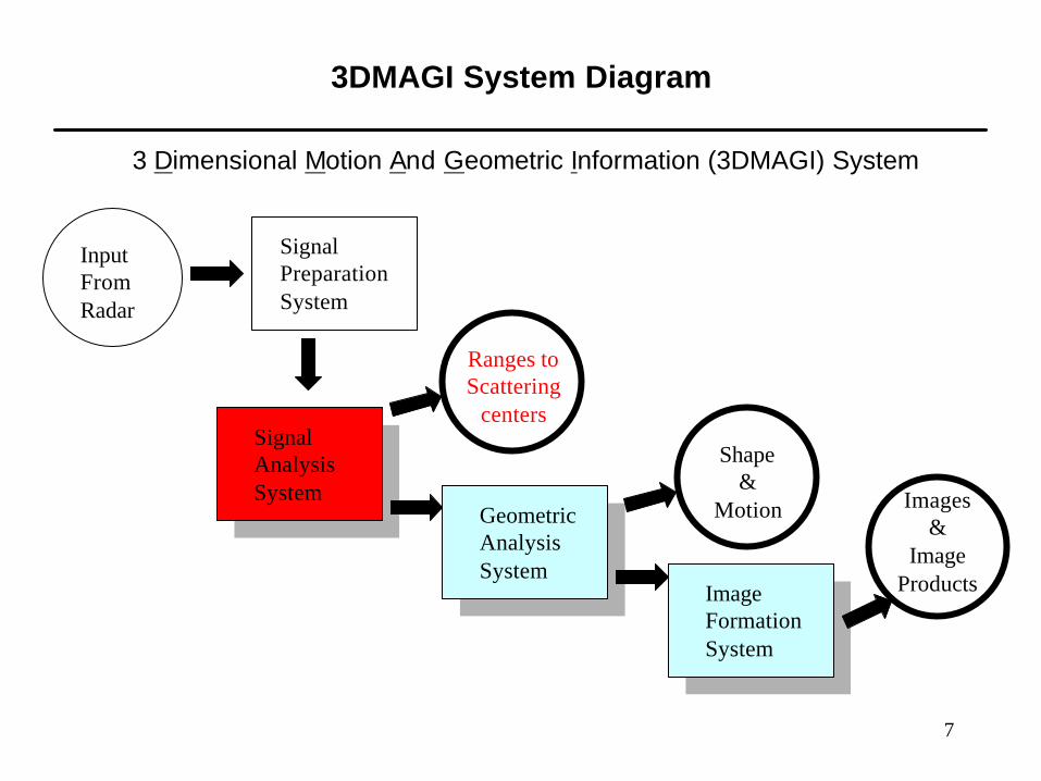
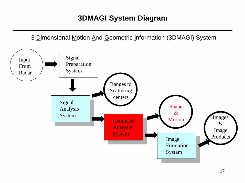
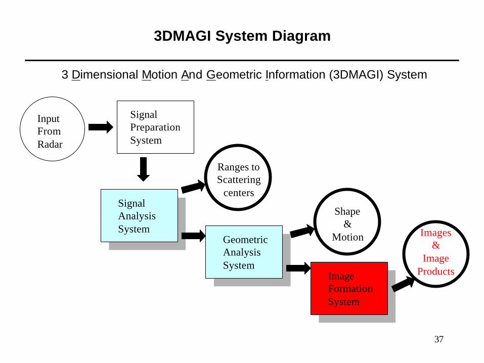
3DMAGI System Diagram
SignalPreparationSystem
InputFromRadar
Signal AnalysisSystem
GeometricAnalysisSystem
ImageFormationSystem
Shape&
Motion Images&
ImageProducts
3 Dimensional Motion And Geometric Information (3DMAGI) System
Ranges toScattering
centers
8
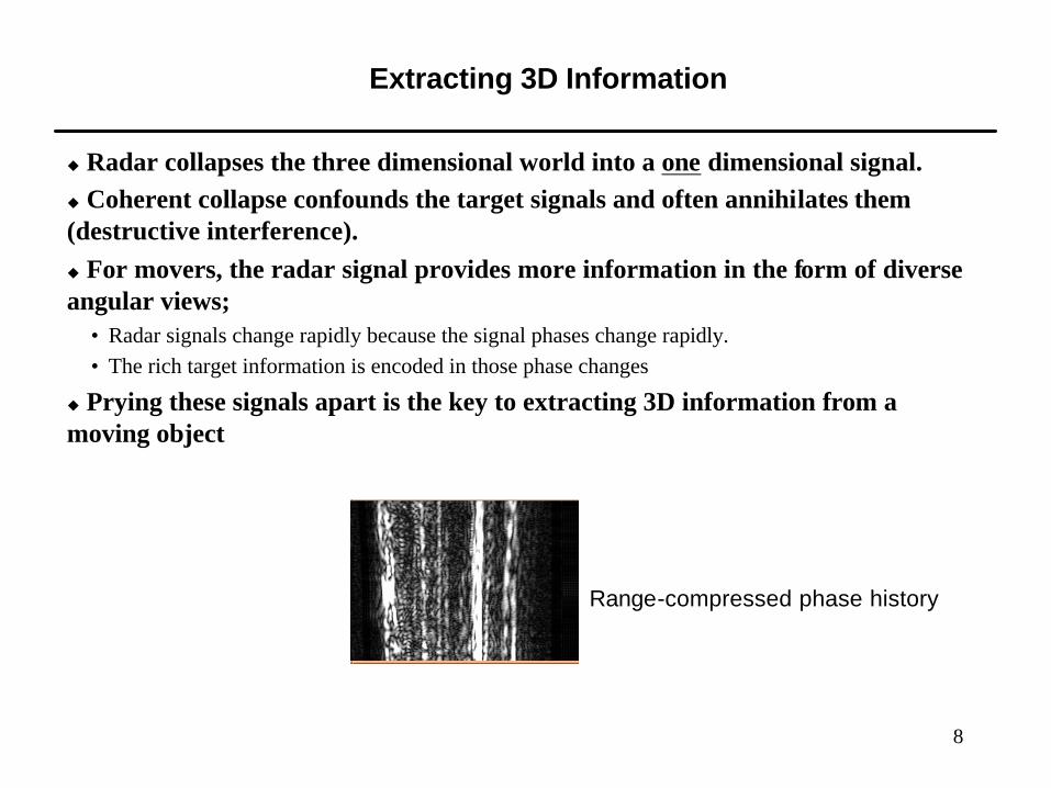
Extracting 3D Information
u Radar collapses the three dimensional world into a one dimensional signal.u Coherent collapse confounds the target signals and often annihilates them (destructive interference).u For movers, the radar signal provides more information in the form of diverse angular views;
• Radar signals change rapidly because the signal phases change rapidly.• The rich target information is encoded in those phase changes
u Prying these signals apart is the key to extracting 3D information from a moving object
Range-compressed phase history
9
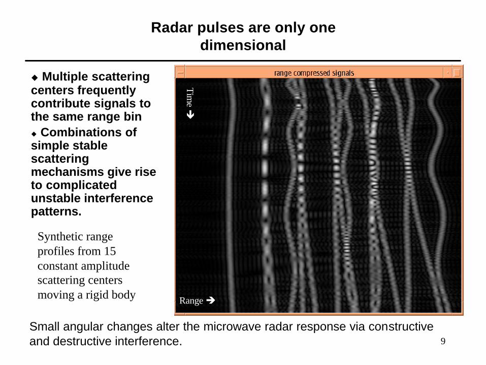
Radar pulses are only one dimensional
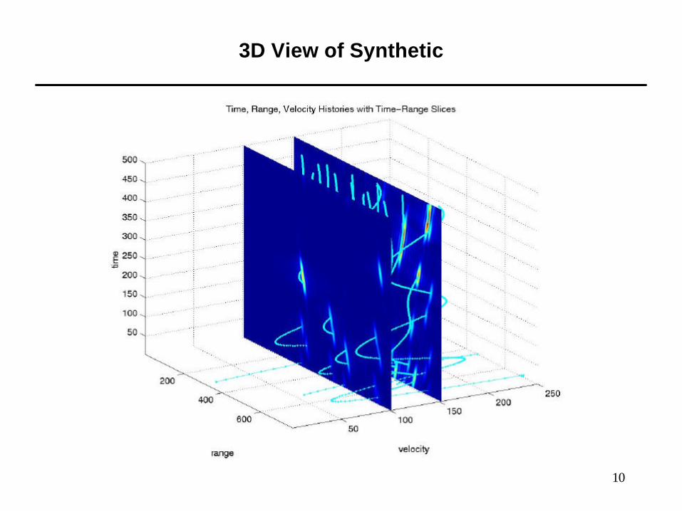
u Multiple scattering centers frequently contribute signals to the same range binu Combinations of simple stable scattering mechanisms give rise to complicated unstable interference patterns.
Range è
Time è
Time è
Synthetic range profiles from 15 constant amplitude scattering centers moving a rigid body
Time è
Small angular changes alter the microwave radar response via constructive and destructive interference.
10
3D View of Synthetic
11
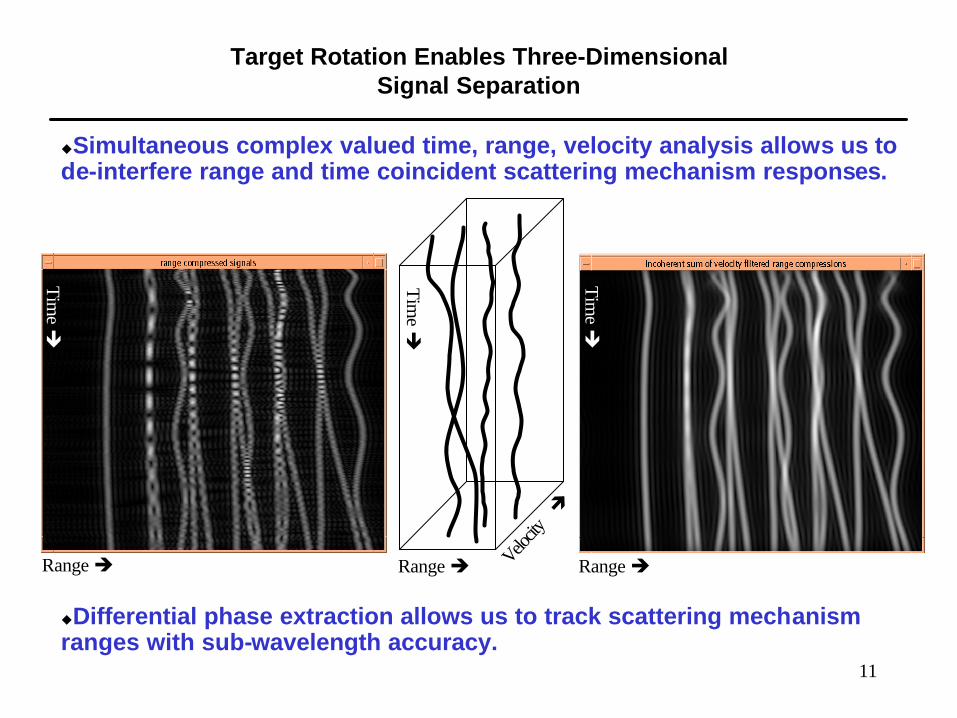
Target Rotation Enables Three-Dimensional Signal Separation
uSimultaneous complex valued time, range, velocity analysis allows us to de-interfere range and time coincident scattering mechanism responses.
uDifferential phase extraction allows us to track scattering mechanism ranges with sub-wavelength accuracy.
Range èRange è Range èVelocity
è
Time è
Time è
Time è
12
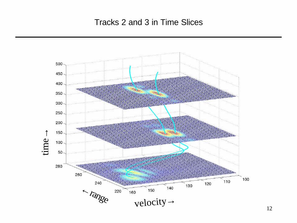
Tracks 2 and 3 in Time Slices
time→
←range velocity→
13
Dynamic progamming method automates optimal track extraction
u The globally optimal path is guaranteed for each passu Several locally optimal paths per pass, in practiceu Optimizing over exponentially many possible trajectories in linear computational complexityu Decisions depend on the integrated scores over the entire dwell; this enables success at lower signal to noise ratiosu Natural tendency to find scattering mechanisms well spread around on the targetu Natural opportunity to enforce continuous differentiabilityu Any local optimality score can be used; phase information can be exploited
14
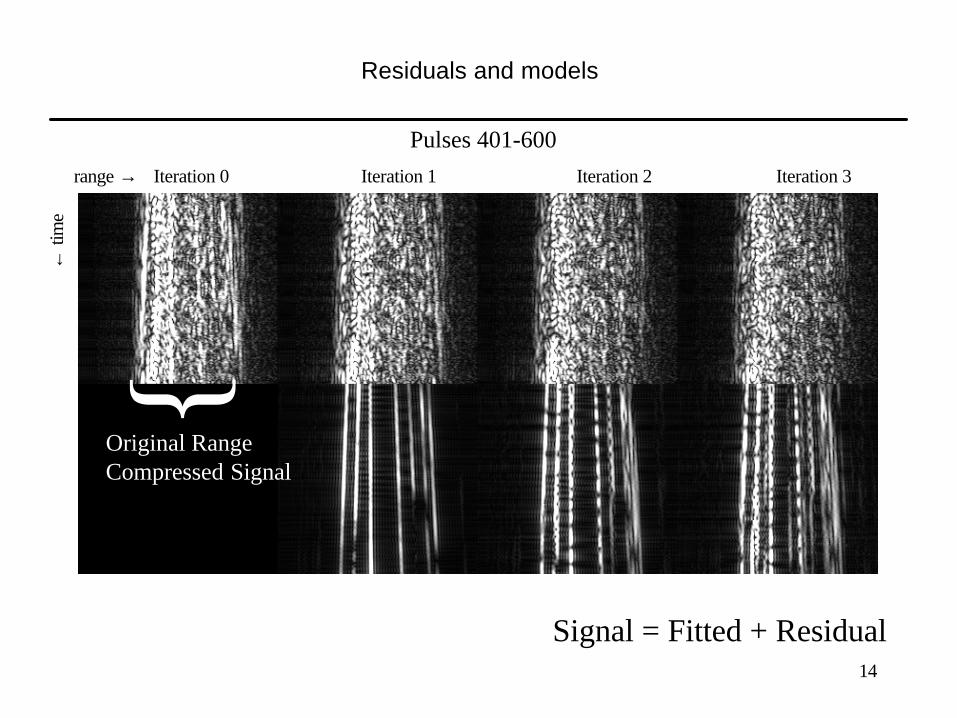
Residuals and models
range →
←tim
e
Pulses 401-600
Signal = Fitted + Residual
Iteration 0 Iteration 1 Iteration 2 Iteration 3
Original Range Compressed Signal
15
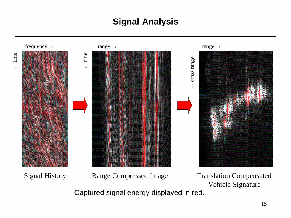
Signal Analysis
Signal History Range Compressed Image Translation Compensated Vehicle Signature
Captured signal energy displayed in red.
←tim
e
←tim
e
frequency → range → range →
←cr
oss
rang
e

16
Three-dimensional signal separation yields range histories with sub-wavelength precision
35 feet
3 feet
17
3DMAGI System Diagram
SignalPreparationSystem
InputFromRadar
Signal AnalysisSystem
GeometricAnalysisSystem
ImageFormationSystem
Shape&
Motion Images&
ImageProducts
3 Dimensional Motion And Geometric Information (3DMAGI) System
Ranges toScattering
centers

18
Rigid Body Kinematics
Consider a configuration of Q points (landmarks) on a moving rigid body:Coordinates at time t
Rotation matrix at time t
Coordinates at time zero
Translation vector at time t
What if we can only observe one of the three coordinates?
Line of sight translation at time t
Far field range at time t
Illumination direction at time t
Fixed 3D coordinates
19
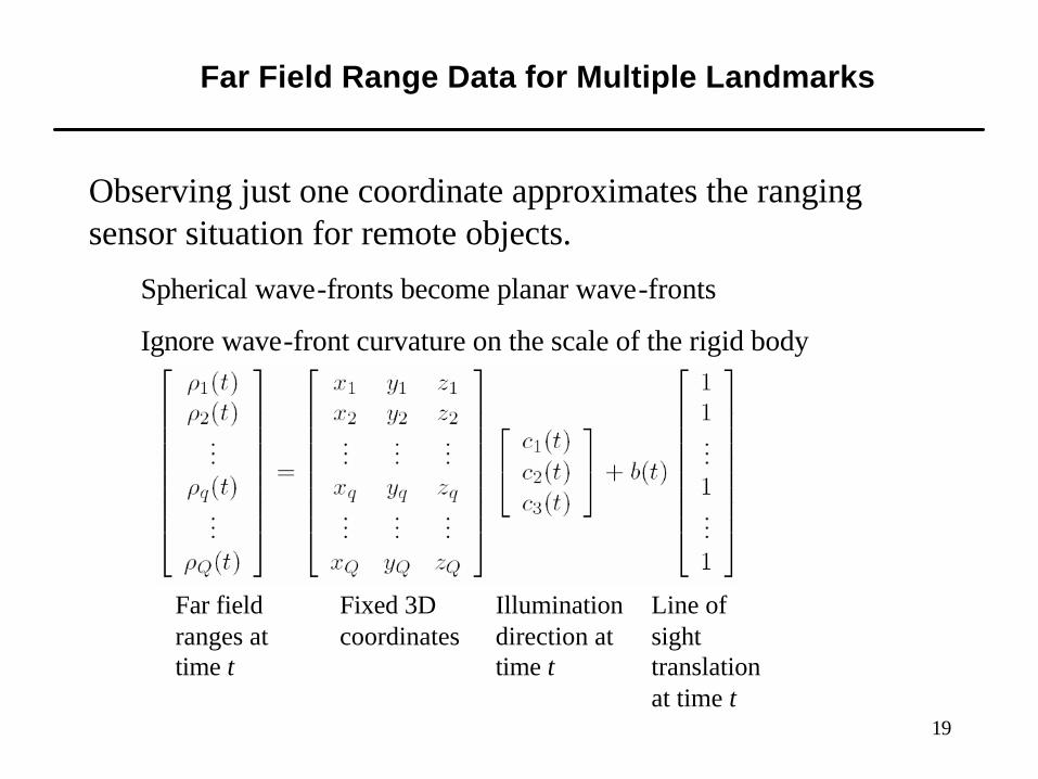
Far Field Range Data for Multiple Landmarks
Observing just one coordinate approximates the ranging sensor situation for remote objects.
Spherical wave-fronts become planar wave-fronts
Ignore wave-front curvature on the scale of the rigid body
Line of sight translation at time t
Far field ranges at time t
Illumination direction at time t
Fixed 3D coordinates

20
Special Cases of the Geometric Inverse Problem
u The ranges are observed data (or are estimated from observed data).u If the motions are known, then solving for the coordinates of the configuration leads to a linear regression problem.u If the coordinates are known, then solving for the motions (illumination directions and line of sight translation) leads toanother linear regression problem.
u What if the motions and coordinates are both unknown?• A nonlinear estimation problem• Non-trivial uniqueness question (well-posedness, identifiability) • The number of unknowns grows with the number of observations
21
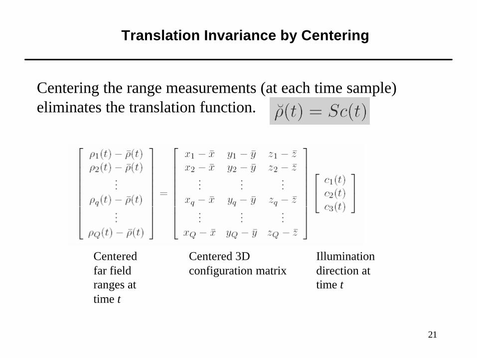
Translation Invariance by Centering
Centering the range measurements (at each time sample) eliminates the translation function.
Centered far field ranges at time t
Illumination direction at time t
Centered 3D configuration matrix
22
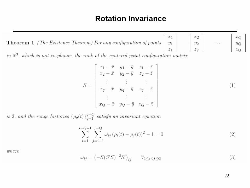
Rotation Invariance
23
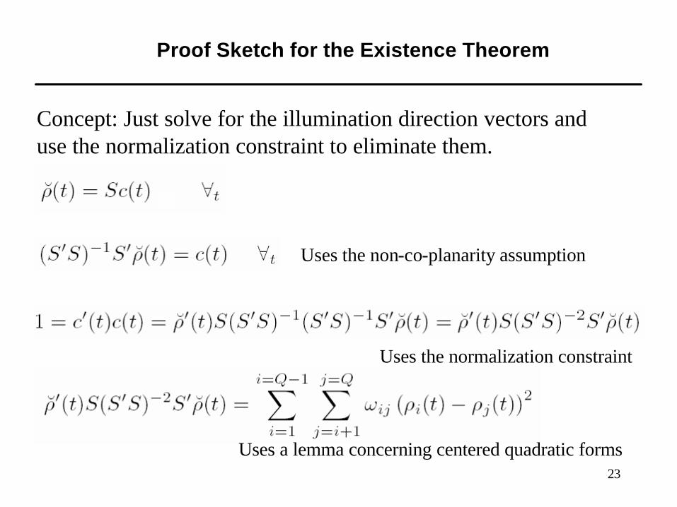
Proof Sketch for the Existence Theorem
Concept: Just solve for the illumination direction vectors and use the normalization constraint to eliminate them.
Uses the non-co-planarity assumption
Uses the normalization constraint
Uses a lemma concerning centered quadratic forms

24
How We Want to Use the Invariant Equation
Try to create an over-determined set of equations for the invariants:
Problems:
Matrix rank never exceeds 6 (S has rank 3, so centered range histories have rank 3, so quadratic combinations of range histories span, at most, 6 dimensions),
Motion must escape any elliptic cone to reach rank 6,
For Q > 4, we need another condition to identify the invariants.
25
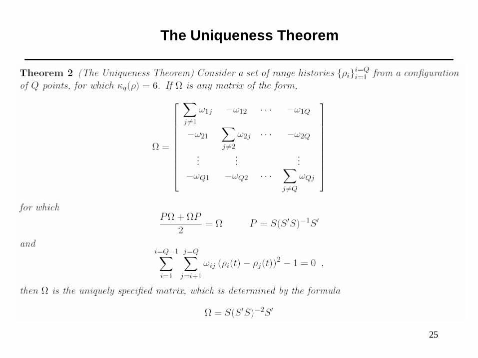
The Uniqueness Theorem
26
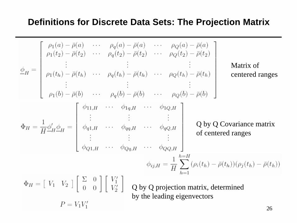
Definitions for Discrete Data Sets: The Projection Matrix
Matrix of centered ranges
Q by Q Covariance matrix of centered ranges
Q by Q projection matrix, determined by the leading eigenvectors
27
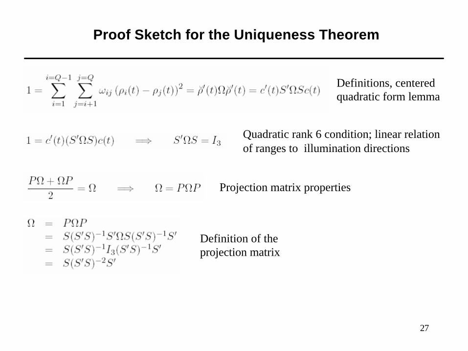
Proof Sketch for the Uniqueness Theorem
Definitions, centered quadratic form lemma
Quadratic rank 6 condition; linear relation of ranges to illumination directions
Projection matrix properties
Definition of the projection matrix

28
Estimation Strategy
29
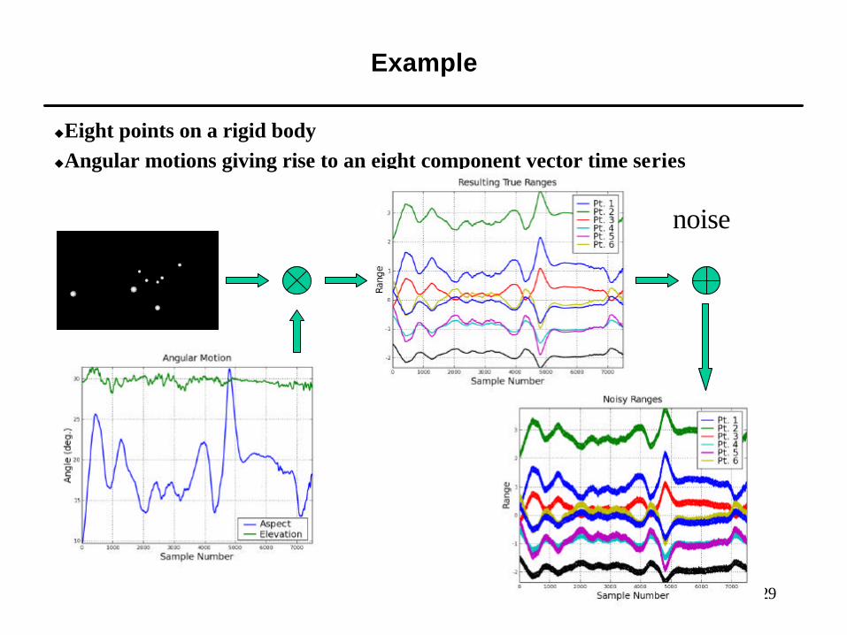
Example
uEight points on a rigid bodyuAngular motions giving rise to an eight component vector time series
noise
30
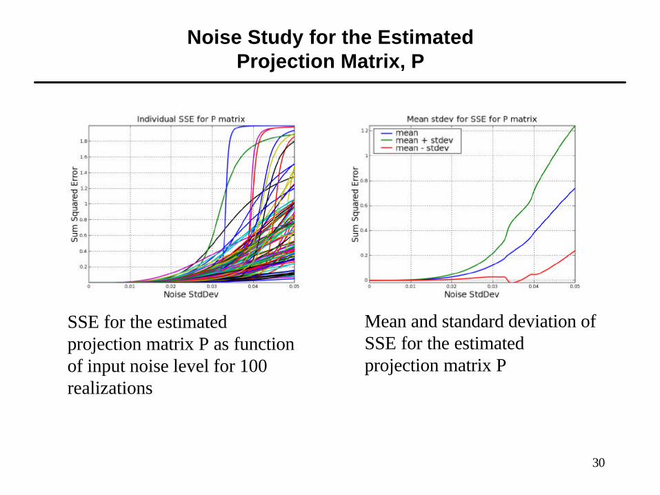
Noise Study for the Estimated Projection Matrix, P
Mean and standard deviation of SSE for the estimated projection matrix P
SSE for the estimated projection matrix P as function of input noise level for 100 realizations
31
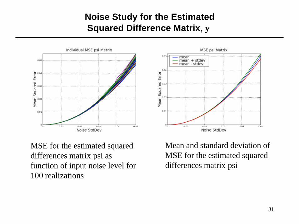
Noise Study for the Estimated Squared Difference Matrix, ψ
Mean and standard deviation of MSE for the estimated squared differences matrix psi
MSE for the estimated squared differences matrix psi as function of input noise level for 100 realizations
32
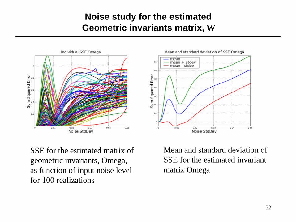
Noise study for the estimated Geometric invariants matrix, Ω
Mean and standard deviation of SSE for the estimated invariant matrix Omega
SSE for the estimated matrix of geometric invariants, Omega, as function of input noise level for 100 realizations
33
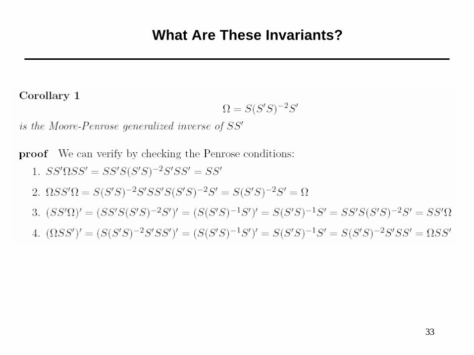
What Are These Invariants?
34
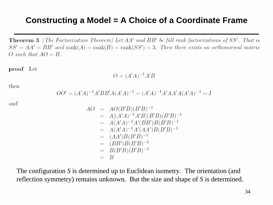
Constructing a Model = A Choice of a Coordinate Frame
The configuration S is determined up to Euclidean isometry. The orientation (and reflection symmetry) remains unknown. But the size and shape of S is determined.

35
Scattering center locations extracted from radar signals
Show movie here

36
Constructing a Model = A Choice of a Coordinate Frame
Low noise
High noise
Estimated point coordinates for three realizations of noise (blue, green, red)
37
3DMAGI System Diagram
SignalPreparationSystem
InputFromRadar
Signal AnalysisSystem
GeometricAnalysisSystem
ImageFormationSystem
Shape&
Motion Images&
ImageProducts
3 Dimensional Motion And Geometric Information (3DMAGI) System
Ranges toScattering
centers
38
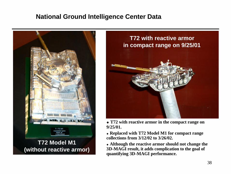
National Ground Intelligence Center Data
T72 with reactive armorin compact range on 9/25/01
T72 Model M1(without reactive armor)
u T72 with reactive armor in the compact range on 9/25/01.u Replaced with T72 Model M1 for compact range collections from 3/12/02 to 3/26/02.u Although the reactive armor should not change the 3D-MAGI result, it adds complication to the goal of quantifying 3D-MAGI performance.
39
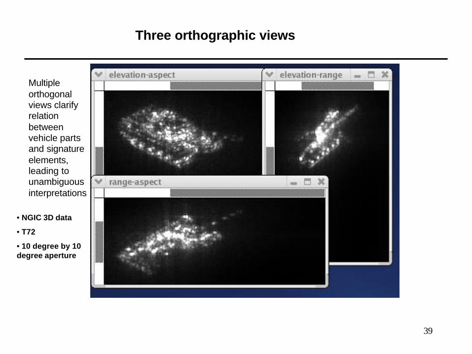
Three orthographic views
Multiple orthogonal views clarify relation between vehicle parts and signature elements, leading to unambiguous interpretations
• NGIC 3D data
• T72
• 10 degree by 10 degree aperture
40
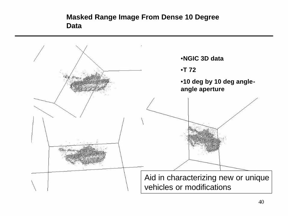
Masked Range Image From Dense 10 Degree Data
•NGIC 3D data
•T 72
•10 deg by 10 deg angle-angle aperture
Aid in characterizing new or uniquevehicles or modifications

41
3D Image Surface

42
Moving target signal history formatted in three dimensions
•Signal history extracted from NGIC t72 data
•TEL motion data quantized to NGIC illumination angles
•Dragnet II Collection
•China Lake
•6 seconds collection time
Fz
?Fy ?
43
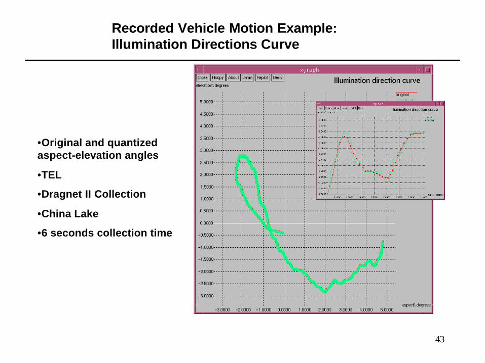
Recorded Vehicle Motion Example: Illumination Directions Curve
•Original and quantized aspect-elevation angles
•TEL
•Dragnet II Collection
•China Lake
•6 seconds collection time
44
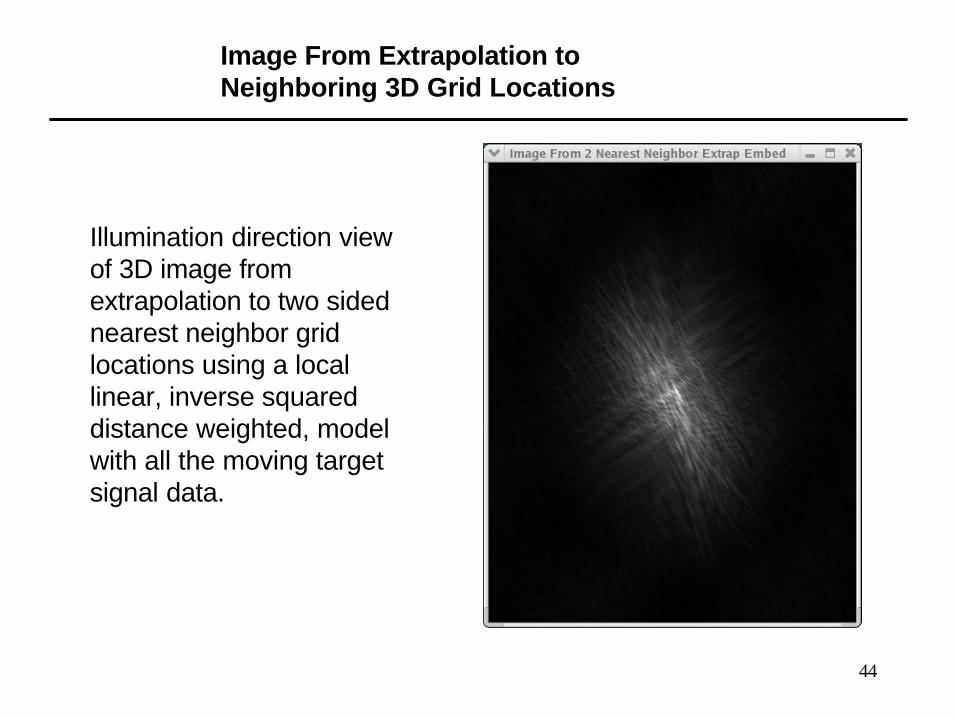
Image From Extrapolation to Neighboring 3D Grid Locations
Illumination direction view of 3D image from extrapolation to two sided nearest neighbor grid locations using a local linear, inverse squared distance weighted, model with all the moving target signal data.
45
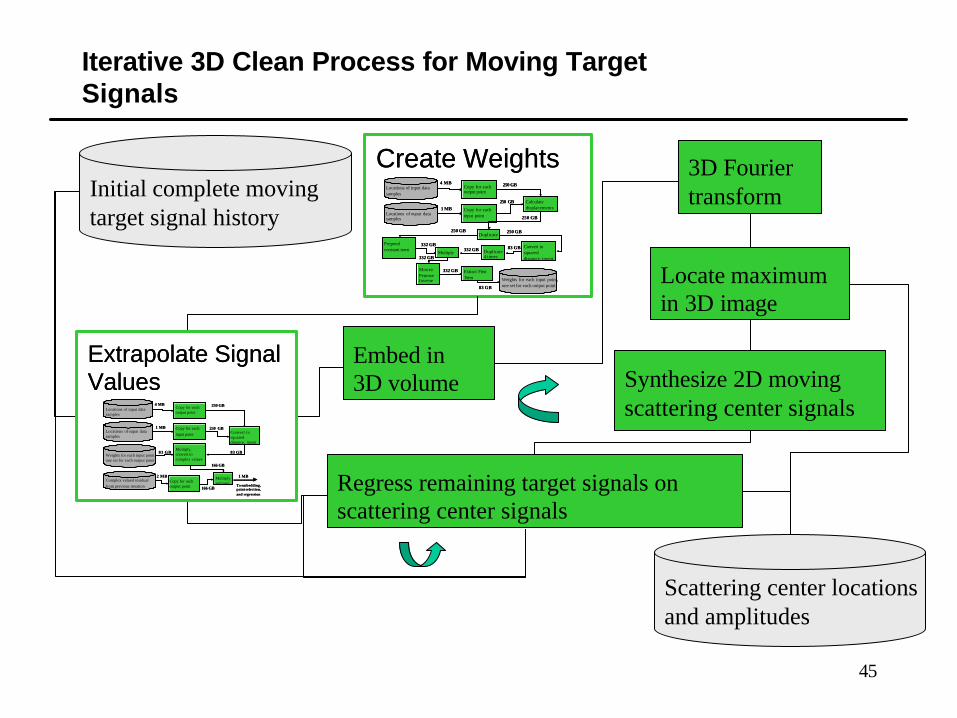
Iterative 3D Clean Process for Moving Target Signals
Copy for each input point
Locations of input data samples
Locations of ouput data samples
Copy for each output point
4 MB
1 MBCalculate displacements
250 GB
250 GB
Prepend constant term
250 GB
Convert to squared distance, invert
250 GBDuplicate
250 GB
332 GBDuplicate 4 times
83 GBMultiply
332 GB
Moore-Penrose Inverse
332 GB
Extract First Term Weights for each input point,
one set for each output point
332 GB
83 GB
Create Weights
Embed in 3D volume
3D Fourier transform
Locate maximum in 3D image
Synthesize 2D moving scattering center signals
Regress remaining target signals on scattering center signals
Initial complete moving target signal history
Weights for each input point, one set for each output point
83 GB
Copy for each input point
Locations of input data samples
Locations of ouput data samples
Copy for each output point
4 MB
1 MBConvert to squared distance, invert
250 GB
250 GB
Multiply, convert to complex values
166 GB
Complex valued residual from previous iteration
Copy for each output point
2 MB Multiply and sum
83 GB
166 GB
1 MB
To embedding, point selection, and regression
Extrapolate Signal Values
Scattering center locations and amplitudes
46
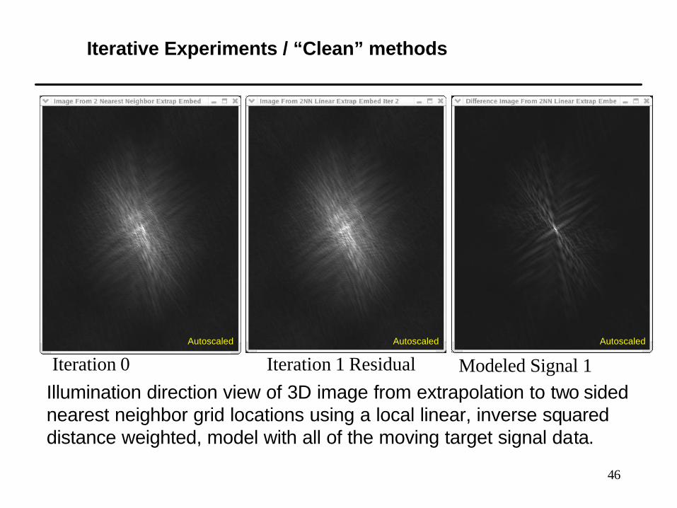
Iterative Experiments / “Clean” methods
Illumination direction view of 3D image from extrapolation to two sided nearest neighbor grid locations using a local linear, inverse squared distance weighted, model with all of the moving target signal data.
Iteration 0 Iteration 1 Residual Modeled Signal 1AutoscaledAutoscaledAutoscaled
47
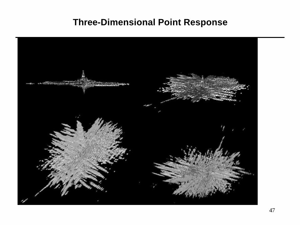
Three-Dimensional Point Response
48
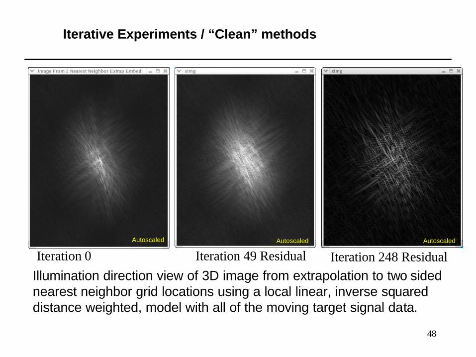
Iterative Experiments / “Clean” methods
Illumination direction view of 3D image from extrapolation to two sided nearest neighbor grid locations using a local linear, inverse squared distance weighted, model with all of the moving target signal data.
Iteration 0 Iteration 49 Residual Iteration 248 ResidualAutoscaled Autoscaled Autoscaled
49
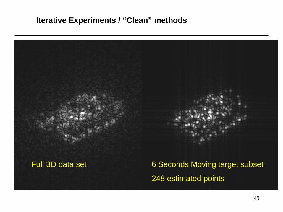
Iterative Experiments / “Clean” methods
Full 3D data set 6 Seconds Moving target subset
248 estimated points
50
Summary
u Moving targets impose 3D information on SAR radar returnsu This extra information confuses any process that does not take it specifically into accountu To take advantage of the 3d information, the motion of the target is needed
• This cannot be predicted, so must be measured
u With the motion information the proper relationships between the target and the data can be determinedu From this data 3D images are possible and are useful for exploiting moving targetsu More research must be done to improve the methods for creating the 3D image products