Using interferometry to measure CMB polarization - …ccapp.osu.edu/workshops/RadioSim2/talks/08-le-zhang-cmb-ohio.pdf · Using interferometry to measure CMB polarization ... provided

Using interferometry to measure CMB polarization

Le Zhang

Interferometric Techniques for Impulsive Signals at Radio/Microwave Frequencies

CCAPP 2013.4.23 based on: arXiv:1209.2930; 1209.2676

Thursday, April 25, 13

http://arxiv.org/abs/1302.6608




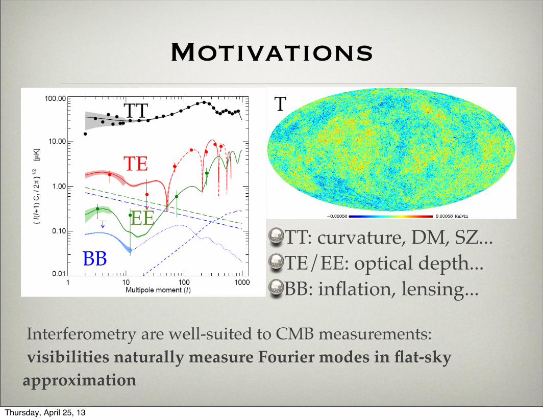
Motivations

TT

TE

EE

BB

T

TT: curvature, DM, SZ...TE/EE: optical depth... BB: inflation, lensing...

Interferometry are well-suited to CMB measurements: visibilities naturally measure Fourier modes in flat-sky approximation


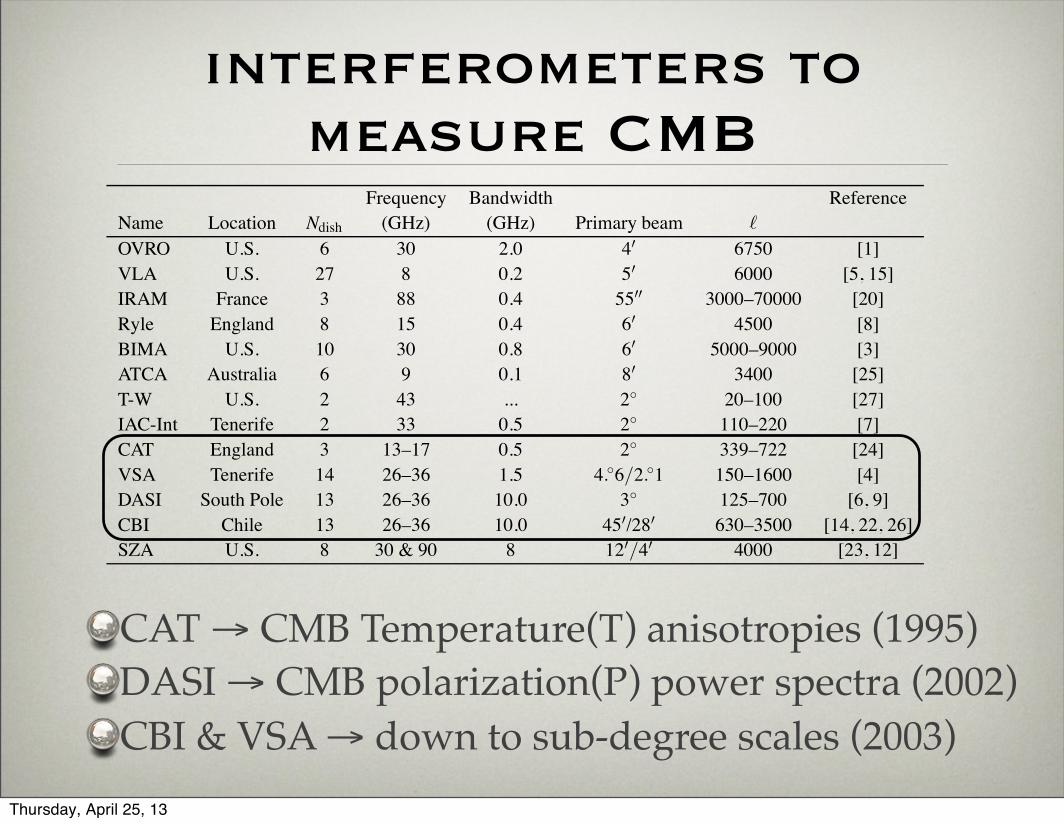
interferometers to measure CMB CMB interferometry Clive Dickinson

Frequency Bandwidth ReferenceName Location Ndish (GHz) (GHz) Primary beam !

OVRO U.S. 6 30 2.0 4! 6750 [1]VLA U.S. 27 8 0.2 5! 6000 [5, 15]IRAM France 3 88 0.4 55!! 3000–70000 [20]Ryle England 8 15 0.4 6! 4500 [8]BIMA U.S. 10 30 0.8 6! 5000–9000 [3]ATCA Australia 6 9 0.1 8! 3400 [25]T-W U.S. 2 43 ... 2" 20–100 [27]IAC-Int Tenerife 2 33 0.5 2" 110–220 [7]CAT England 3 13–17 0.5 2" 339–722 [24]VSA Tenerife 14 26–36 1.5 4."6/2."1 150–1600 [4]DASI South Pole 13 26–36 10.0 3" 125–700 [6, 9]CBI Chile 13 26–36 10.0 45!/28! 630–3500 [14, 22, 26]SZA U.S. 8 30 & 90 8 12!/4! 4000 [23, 12]

Table 2: Summary of interferometric experiments to measure CMB anisotropies. This is an update of aprevious version of this table produced by [30].

only given to utilise a single 1.5GHz channel. The VSA was carefully designed to minimise allsystematics, both instrumental and astrophysical. The entire telescope was located inside a largeground-screen while the tracking elements on the tip-tilt table allowed fringe-rate filtering of non-astronomical signals such as cross-talk and and ground spillover [29]. This proved to be essentialfor observing during the day (to filter out the Sun and Moon) and also for filtering out correlatedsignals that were found to be strong on the shortest baselines. The VSA also employed an additionalsingle-baseline interferometer consisting of two 3.7m dishes located in their own ground screens.This allowed for a survey of the brightest sources in each VSA field (positions were provided froman earlier 15GHz survey of the VSA fields by the Ryle telescope) at the same frequency and at thesame time. The VSA produced accurate measurements of the CMB power spectrum over the range!= 150–1600 [4].

The DASI instrument was located at the South Pole and used 13 20 cm horns located on a tablemounted onto an az-el mount. It operated at 26–36GHz with 10 channel 10GHz digital correlator.Its small horns and table provided good sensitivity over the !-range 140–900 allowing detectionof the first 3 acoustic peaks [6]. DASI was reconfigured to measure CMB polarization, with eachantenna measuring a single polarization (left or right circular). In 2002 DASI obtained the firstdetection of CMB polarization which provided remarkable confirmation of the standard theory ofcosmology [9].

The CBI was located in the Atacama desert, Chile and operated from 1999–2008 and utilisedmany of the same components as its “sister” instrument, DASI. The CBI consisted of 13 0.9mantennas also located on a table that could be moved along 3 axes (az,el,parallactic angle). LikeDASI, the antennas did not track giving a constant coverage in the u,v plane, which was improvedby rotating the telescope in parallactic angle. The CBI utilised the same 10 channel 10GHz digitalcorrelator as was used for DASI. After discussions between the CBI/DASI/VSA groups (circa2000), the CBI group focussed on high-! measurements. The CBI was the first experiment toconvincingly show the drop in power due to the Silk damping tail expected from the standard theory

5

CAT → CMB Temperature(T) anisotropies (1995) DASI → CMB polarization(P) power spectra (2002)CBI & VSA → down to sub-degree scales (2003)


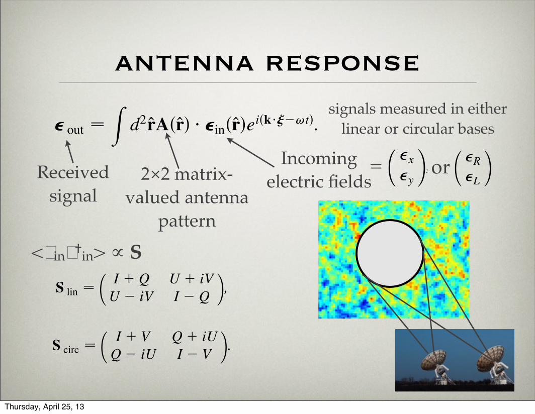
antenna response

data than for maps made with single-dish instruments[35,36].

As we will see, a variety of systematic errors in inter-ferometers can be modeled via Jones matrices [16,37,38]and by deviations of the antenna patterns (including cross-polar contributions) from assumed ideal forms. We willassume that each of these errors can be characterized bysmall unknown parameters, such as gain fluctuations, crosstalk between detectors, pointing errors, etc. We will firstcalculate the effect of each error on the measured visibil-ities. We will then provide a method of quantifying theeffects of each of these errors on estimates of the polariza-tion power spectra CEl , CBl that can be obtained from ahypothetical data set.

This paper has the following structure. Section IIpresents the mathematical formalism we will use to de-scribe interferometric visibilities for polarization data.Section III presents the effects of various systematic errorson the visibilities extracted from a hypothetical CMBexperiment. Section IV presents a method of forecastingerrors on power spectrum estimates from errors on visibil-ities. Sections V and VI contain results showing how theerror forecasts on both E and B power spectra depend onthe parameters that characterize the various systematicerrors. Section VII summarizes these results, comparesthem with simulations, and concludes with a discussionof the implications. A brief appendix contains a usefulmathematical result.

Sections IV, V, and VI contain quite a bit of technicaldetail. The particularly busy or impatient reader shouldnote that the key ideas of Sec. IV are summarized at thebeginning, and the final results of Secs. V and VI aresummarized in Sec. VII and Table I.

II. FORMALISM

A. Antenna patterns and visibilities

In this section we review some basic properties of CMBinterferometric polarimetry and establish some notation. Amore detailed introduction to interferometry may be foundin [39], and [37] provides a useful guide to astronomicalpolarimetry.

We begin by considering some properties of the individ-ual antennas in our hypothetical interferometer. Supposethat each element of our interferometer is designed tomeasure two polarization states (say, horizontal and verti-cal polarizations or right and left circular polarizations).We can model the response of this antenna as

! out !Zd2rA"r# $ !in"r#ei"k$"%!t#: (2.1)

Here !in"r# is the electric field of the incoming radiationfrom direction r, and !out is a two-component vector givingthe two measurements. The vector " is the location of theantenna, and A is a matrix-valued antenna pattern. Thewave vector and frequency are k and !. (We assumemonochromatic radiation for simplicity.) In a particularexperiment, only one output from each antenna may bemeasured. In these cases, we can simply ignore the othercomponent of !out.

Throughout this paper, we will consider experiments inwhich the beam width is small enough that the flat-skyapproximation is appropriate in analyzing any single point-ing of the instrument. (Mosaicking of multiple pointings ofsuch an instrument, in which this approximation may notbe valid, is considered in [30].) In that case, we canrepresent the direction r by a vector in the plane (specifi-cally, the tangent plane to the sphere at the pointing center)with components "x; y#.

We can of course express the components of the vectors!in and !out in any basis we like. In particular, we canresolve these vectors in either a linear polarization basiswith components "!x; !y# or a right and left circular basiswith components "!R; !L#. The two bases are related by aunitary transformation

!R!L

! "! Rcirc $

!x!y

! "; (2.2)

with

R circ !1###2p 1 i

1 %i! "

: (2.3)

In either case, an ideal antenna, i.e., one with equal re-

FIG. 1. Power spectra for temperature anisotropy (T), TE cross-correlation (X, absolute value plotted), E-type polarization, andB-type polarization. The best-fit parameters from the three-year WMAP data were used [42] with a tensor-to-scalar ratio T=S ! 0:01.The right panel shows the ratios of the power spectra.

EMORY F. BUNN PHYSICAL REVIEW D 75, 083517 (2007)

083517-2

Received signal

2×2 matrix-valued antenna

pattern

Incoming electric fields

signals measured in either linear or circular bases

sponse to both polarization states and no mixing betweenthem, would have A equal to a scalar function A!r" timesthe identity matrix. Since these antenna patterns apply toelectric fields, not intensities, the intensity beam pattern isjAj2.

We now move on from consideration of individual an-tennas to the visibilities formed from pairs of antennas.Consider an interferometer with N antennas. The outputsignal from antenna jwill be denoted !!j"out. As noted earlier,we will treat this as a two-component vector with compo-nents !!j"out , with m # X, Y for a linear polarization experi-ment or m # R, L for a circular-polarization experiment.Each of the measured visibilities is obtained by correlatinga component of !out from one antenna with a componentfrom another antenna: V!jk"mn # h!!j"out m!

!k"$out ni. For a fixed pair

of antennas (jk), the visibilities form a 2% 2 matrix V!jk",which is related to the Stokes parameter matrix as follows:

V !jk" #Zd2rA!j"!r" & S!r" &A!k"y!r"e'2"iujk&r: (2.4)

Here the A’s are the antenna patterns for the two antennas,and the baseline vector ujk # !"!k" ' "!j""=# is the sepa-ration between the two antennas in units of wavelength.The matrix Ay is the Hermitian conjugate of A. The 2% 2Stokes parameter matrix S is proportional to h!in i! $

in ji. Inthe linear and circular-polarization bases, it is given by

S lin #I (Q U( iVU' iV I 'Q

! "; (2.5)

S circ #I ( V Q( iUQ' iU I ' V

! ": (2.6)

In an ideal experiment with A proportional to the iden-tity matrix (no cross-polar response and identical copolarresponse to both polarization states), V!jk" / S. In otherwords, each visibility measures a simple linear combina-tion of the Stokes parameters. To be explicit, let us defineStokes visibilities

V!jk"Z )Zd2rA!j"!r"Z!r"A!k"!r"e'2"iujk&r; (2.7)

where Z # I, Q, U, V is a Stokes parameter. As is wellknown, these can also be written as a convolution inFourier space:

V!jk"Z /Zd2k ~Z!k" ~A$

jk!k' 2"u" (2.8)

with Ajk # A!j"A!k".A polarimetric interferometer can work either by inter-

fering linear polarization states or circular-polarizationstates. Throughout this paper, we will refer to these possi-bilities as linear experiments and circular experiments,respectively. Information about both linear and circular

polarization can be obtained from either type ofexperiment.

In an ideal linear experiment, we would extract theStokes parameters from the visibility matrix as follows:

VI #12!VXX ( VYY"; (2.9a)

VQ #12!VXX ' VYY"; (2.9b)

VU #12!VXY ( VYX"; (2.9c)

VV #12i!VXY ' VYX": (2.9d)

Here we are assuming that all antennas split up the incom-ing radiation into orthogonal linear polarizations with re-spect to a single fixed coordinate system !X; Y". Thesuperscript (jk) is suppressed.

For the weak polarization found in CMB data, Eq. (2.9b)is not a practical way to measure Stokes Q because itrequires perfect cancellation of the much larger I contri-butions; in practice, such an experiment measures linearpolarization only via U, not Q. Since Q! U under a 45*

rotation, we measure Q in practice by using antennas thatmeasure linear polarization states in a basis !X0; Y0" that isrotated with respect to !X; Y". This can be done either byrotating the instrument or by having the polarizers ondifferent antennas oriented in different ways. In eithercase, note that in general the Stokes parameters Q, U arenot generally measured with the same baseline at the sametime.

The corresponding relations in a circular experiment are

VI #12!VRR ( VLL"; (2.10a)

VQ #12!VRL ( VLR"; (2.10b)

VU #12i!VRL ' VLR"; (2.10c)

VV #12!VRR ' VLL": (2.10d)

In a circular experiment, both Q and U visibilities can bemeasured simultaneously on a single baseline.

We do not expect any cosmological source of circularpolarization: Stokes V is expected to be zero. Nonetheless,it may be useful to measure the Stokes visibility VV as amonitor of systematic errors. Conversely, if a noncosmo-logical source of circular polarization is present, system-atic errors may cause it to contribute to measurements oflinear polarization.

B. Modeling systematic errors

A wide variety of systematic errors can be modeled asimperfections in the matrix-valued antenna patterns of theantennas. We will model these errors in the following way:

SYSTEMATIC ERRORS IN COSMIC MICROWAVE . . . PHYSICAL REVIEW D 75, 083517 (2007)

083517-3





II. FORMALISM








!R!L

! "! Rcirc $

!x!y

! "; (2.2)

with

R circ !1###2p 1 i

1 %i! "

: (2.3)




083517-2





II. FORMALISM








!R!L

! "! Rcirc $

!x!y

! "; (2.2)

with

R circ !1###2p 1 i

1 %i! "

: (2.3)




083517-2

= or

<"in"†in> ∝ S


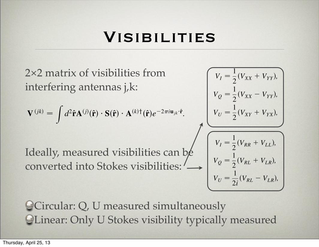
Visibilitiessponse to both polarization states and no mixing betweenthem, would have A equal to a scalar function A!r" timesthe identity matrix. Since these antenna patterns apply toelectric fields, not intensities, the intensity beam pattern isjAj2.








! "; (2.5)


! ": (2.6)





jk!k' 2"u" (2.8)





VI #12!VXX ( VYY"; (2.9a)

VQ #12!VXX ' VYY"; (2.9b)

VU #12!VXY ( VYX"; (2.9c)

VV #12i!VXY ' VYX": (2.9d)





VI #12!VRR ( VLL"; (2.10a)

VQ #12!VRL ( VLR"; (2.10b)

VU #12i!VRL ' VLR"; (2.10c)

VV #12!VRR ' VLL": (2.10d)






083517-3









! "; (2.5)


! ": (2.6)





jk!k' 2"u" (2.8)





VI #12!VXX ( VYY"; (2.9a)

VQ #12!VXX ' VYY"; (2.9b)

VU #12!VXY ( VYX"; (2.9c)

VV #12i!VXY ' VYX": (2.9d)





VI #12!VRR ( VLL"; (2.10a)

VQ #12!VRL ( VLR"; (2.10b)

VU #12i!VRL ' VLR"; (2.10c)

VV #12!VRR ' VLL": (2.10d)






083517-3









! "; (2.5)


! ": (2.6)





jk!k' 2"u" (2.8)





VI #12!VXX ( VYY"; (2.9a)

VQ #12!VXX ' VYY"; (2.9b)

VU #12!VXY ( VYX"; (2.9c)

VV #12i!VXY ' VYX": (2.9d)





VI #12!VRR ( VLL"; (2.10a)

VQ #12!VRL ( VLR"; (2.10b)

VU #12i!VRL ' VLR"; (2.10c)

VV #12!VRR ' VLL": (2.10d)






083517-3

Circular: Q, U measured simultaneouslyLinear: Only U Stokes visibility typically measured

2×2 matrix of visibilities from interfering antennas j,k:

Ideally, measured visibilities can be converted into Stokes visibilities:


6

(a) I(x) (b) Q(x) (c) U(x)

(d) VI (u) (e) VQ(u) (f) VU (u)

Fig. 1.— Simulated interferometric observations. The images shown in panels (a), (b) and (c) are a 30 ! 30-degree realization of thetwo-dimensional CMB Stokes fields I, Q and U based on the standard CMB power spectra, with a 64 ! 64 pixel grid. All Fourier modeshigher than the Nyquist frequency are filtered out to avoid aliasing. The images shown in the remaining panels are simulated Stokesvisibilities (shown as magnitudes) by a QUBIC-like observation, assuming a Gaussian primary beam A(x) with beam width ! = 5!, asimulated 12-h uv-coverage of single field with 400 close-packed antennas and Gaussian random noise of 0.015µK per visibility. The mapunits are equivalent thermodynamic temperature in µK.

ferences numerically along each parameter direction todirectly obtain the Hessian matrix and then calculatethe statistical error estimates on the band-power spec-tra. We find this procedure requires only about 30 minsof CPU time for ! 4000 visibilities.Fig. 2 shows the resulting maximum-likelihood CMB

power spectra based on the simulated observations inthe absence of systematic errors. The recovered powerspectra are basically consistent with the true underlyingCMB power spectra within 2-!.

4. ANALYSIS OF POINTING ERRORS

Using the simulated Stokes visibilities and applying theML analysis described in the previous section, we ob-tained estimates of the systematic pointing errors in theCMB power spectra. Other systematics, such as beamshape errors, gain errors and cross polarization, will bepresented in a detailed analysis on various instrumentalsystematics in a forthcoming paper.The quadrature di!erence between the recovered power

spectrum with and without pointing errors is used to es-timate the e!ect of systematic pointing errors. Also thepointing errors can potentially change the statistical er-ror (which depends on the curvature of the likelihoodfunction) for a given experiment. The bias in the i-thband-power spectrum Ci and the change in the corre-sponding statistical error !i are given by

"Ci = "(Cerrori # Ci)2$1/2

"!i = "(!errori # !i)

2$1/2 , (19)

where Cerrori refers to values obtained in the presence

of pointing errors and Ci is the recovered power spec-trum for that same patch of the sky in the absence ofsystematic errors (refers to “ML” in Fig. 2). To quan-

tify how significant this systematic error is when com-pared with the systematics-free 1-! statistical error, fol-lowing O’Dea et al. (2007) and Miller et al. (2008), weintroduce the tolerance parameters defined by

"i ="Ci!i

#i ="!i

!i, (20)

where "Ci and "!i are quadrature di!erences in Eq. 19.We set up a tolerance limit, say 10%, which requires thatneither " nor # exceed 0.1. In our simulations, we con-sider two types of pointing errors, which we call uncorre-lated and fully-correlated. In the uncorrelated case, thepointing errors are assumed to be Gaussian-distributedfor each antenna (and tend to average out), and in thefully-correlated case, the pointing o!sets "x relative tothe desired observing direction are identical for all theantennas and remain fixed on the sky as the sky ro-tates. Note this situation is di!erent from the case ofa misalignment of the entire interferometer by "x fromthe expected direction, where the observed patch wouldchange as the sky rotates.As introduced by Bunn (2007), we use an error pa-

rameter p in units of the beam width ! to characterizethe pointing error level, i.e., p = $/! and p = |"x|/! re-spectively for the uncorrelated and fully-correlated cases,where $ is the root-mean-square (rms) value of Gaussian-distributed pointing errors and |"x| is the amplitude ofidentical pointing o!sets. For clear comparison, Fig. 3shows the values of " and # in the BB, TB and EBpower spectra with the identical p = 0.1 for both thecases. As illustrated in Fig. 3 for the uncorrelated case,the parameter " in each band-power bin for the BB

~1/σ

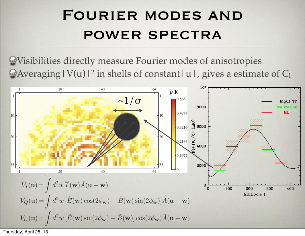
Fourier modes and power spectra

Visibilities directly measure Fourier modes of anisotropiesAveraging|V(u)|2 in shells of constant|u|, gives a estimate of Cl

8

(a) TT power spectrum (b) EE power spectrum (c) BB power spectrum

(d) TE power spectrum (e) TB power spectrum (f) EB power spectrum

Fig. 2.— The CMB power spectra TT,EE,BB, TE, TB,EB (red) recovered by maximizing the likelihood function from a mock QUBIC-like observation in the absence of systematic errors (see details in text). The flat band powers are estimated in 6 bins with bin-widths!u = 9.5 and with 1-! (red hatched) statistical uncertainties. The input CMB power spectra are shown in black and the specific realizationsof such input power spectra are shown in green.

(a) BB power spectrum (b) TB power spectrum (c) EB power spectrum

Fig. 3.— Assessment of systematic pointing error for BB, TB and EB power spectra. In the units of systematics-free 1-! statisticaluncertainties, the solid lines are for the induced bias in the power spectra and dotted for the changes in statistical uncertainties. Greentriangles denote the results in the case of the independent Gaussian-distributed pointing errors with the dispersion " = 0.1! for eachantenna, which are estimated by averaging over 50 simulations. The corresponding analytical result by Bunn (2007) is shown in dashed-black line. Blue points correspond to all the antennas having the identical pointing o"sets with the amplitude |!x| = 0.1! and the resultsare obtained by averaging over 20 random directions relative to the target direction.

3

over the beam. The total e!ect on the visibilities can befound from the relations:

V jk =

!

d2xJj"

Gj(x) · S(x) ·G†k(x)

#

J†ke!2!iujk·x .

(5)For the j-th antenna with gain errors gj1, g

j2 and cross-

talk couplings !j1, !j2, the Jones matrix reads

Jj =

$

1 + gj1 !j1!j2 1 + gj2

%

. (6)

Similar to the Jones matrix, an azimuthally symmetricantenna pattern has the form of

Gj(r,") =

$

Gj0 +

12G

j1 cos(2")

12G

j1 sin(2")

12G

j1 sin(2") Gj

0 ! 12G

j1 cos(2")

%

,

(7)where (r,") are polar coordinates, G0 is the ideal beamshape and G1 leads to two polarization states mixing.The scalar functions G0, G1 depend only on r. Foran ideal interferometer, each antenna has an identicalresponse to both polarization states while there is nomixing between them. In this case, G is equal to ascalar function multiplied by the identity matrix, i.e.,G(x) = G(x)1.For both linear and circular polarization experiments,

coupling errors (!) are the major sources of systemat-ics a!ecting the B-mode power spectrum due to leakagefrom I into Q and U , while less worrisome gain errorswould mix VQ and VU with each other. Furthermore, asshown by Bunn (2007), the visibility for Stokes V couldprovide a useful diagnostic to monitor the presence ofthese systematics.For simplicity we assume that instrument errors in the

Jones matrix are negligible (taking J = 1) and each an-tenna has identical beam patterns for both polarizationstates and has no cross-polar response (i.e., o!-diagonalentries in G). Then, each visibility measures a simplelinear combination of the Stokes parameters. We canextract Stokes visibilities from Eq. 2, yielding

V jkZ =

!

d2xZ(x)Gj(x)G"k(x)e!2!iujk ·x , (8)

for Z = {I,Q, U, V }. Since the visibility function is theFourier transform of the Stokes fields on the sky weightedby the antenna response, by using the well-known con-volution theorem, we can write the visibility function inFourier space (uv-domain):

V jkZ (u) =

!

d2w Z(u!w)Gjk(w) , (9)

where Z(u) and Gjk(u) are the Fourier transforms ofZ(x) and Gj(x)G"k(x), respectively. Note that each an-tenna pattern could di!er from the others because of sys-tematic beam errors.In this study, we only focus on di!erential pointing er-

rors. The pipeline presented in this paper can be appliedin a straightforward manner to other systematics. Point-ing errors occur when not all the antennas point in thesame direction. Following Bunn (2007), we model thepointing error as a Gaussian-distributed error with dis-persion #. Assuming the j-th antenna has the pointing

o!set #xj relative to a desired direction, then accordingto Eq. 8, each visibility can be expressed in the form

V jkZ =

!

d2xZ(x)Gj(x+ #xj)G"k(x+ #xk)

"e!2!iujk·x , (10)

where Z = {I,Q, U} and the beam response G(x) canbe approximated by a circular Gaussian of a frequency-dependent dispersion $, i.e., G(x) = exp(!|x|2/2$2(%)).The corresponding Fourier transform is thus given byG(u) = 2&$2(%) exp(!2&2|u|2$2(%)).In order to recovery the power spectrum based on sim-

ulated visibility data, one needs to construct the covari-ance matrix, which is the fundamental tool for analysisof Gaussian random CMB fields. In principle, all kinds ofsystematic errors in visibilities can be simulated throughEq. 5, whereas the theoretically predicted covariance ma-trix does not include any systematic uncertainties. Tak-ing the error-free beam pattern, G, with identical re-sponse between antennas, Eqs. 8 and 9 can be simplifiedas follows:

VZ(u)=

!

d2xZ(x)A(x)e!2!iu·x (11)

VZ(u)=

!

d2w Z(u!w)A(w) . (12)

Here the intensity beam pattern, A(x), is defined by|G(x)|2 and A is its Fourier transform.In the flat-sky approximation, the Stokes parameters

Q and U can be decomposed into the E- and B-modes inFourier space (Zaldarriaga & Seljak 1997). Using Eq. 12,the Stokes visibilities VI , VQ and VU then can be ex-pressed in terms of T , E and B modes as follows:

VQ(u)=

!

d2w [E(w) cos(2"w)! B(w) sin(2"w)]A(u!w)

VU (u)=

!

d2w [E(w) sin(2"w) + B(w)] cos(2"w)A(u!w)

VI(u)=

!

d2w T (w)A(u!w) , (13)

where T , E and B stand for the CMB temperature field,T , and polarization fields, E and B, in Fourier space and"w is the angle made by the vector w with respect to thex-axis. In this study we assume the Stokes visibility VVto be zero.Given a set of visibility measurements, one can use

maximum likelihood analysis to evaluate the CMB powerspectra of the temperature and polarization. By defin-ing a vector of data V # (V 1

I , V1Q, V

1U ; · · · ;V n

I , V nQ , V n

U )at each baseline vector ui with i = 1, . . . , n, the corre-sponding covariance matrices of the CMB visibilities are

CijZZ! #$VZ(ui)V

"Z! (uj)%

=

!

d2w

!

d2w#&

Z(w)Z #"(w#)'

" A(ui !w)A"(uj !w#)

=

!

d2w Szz!(|w|)A(ui !w)A"(uj !w) , (14)

where i, j denote visibility data indices and the depen-dence of the correlation functions Szz! on the CMB

3

over the beam. The total e!ect on the visibilities can befound from the relations:

V jk =

!

d2xJj"

Gj(x) · S(x) ·G†k(x)

#

J†ke!2!iujk·x .

(5)For the j-th antenna with gain errors gj1, g

j2 and cross-

talk couplings !j1, !j2, the Jones matrix reads

Jj =

$

1 + gj1 !j1!j2 1 + gj2

%

. (6)

Similar to the Jones matrix, an azimuthally symmetricantenna pattern has the form of

Gj(r,") =

$

Gj0 +

12G

j1 cos(2")

12G

j1 sin(2")

12G

j1 sin(2") Gj

0 ! 12G

j1 cos(2")

%

,

(7)where (r,") are polar coordinates, G0 is the ideal beamshape and G1 leads to two polarization states mixing.The scalar functions G0, G1 depend only on r. Foran ideal interferometer, each antenna has an identicalresponse to both polarization states while there is nomixing between them. In this case, G is equal to ascalar function multiplied by the identity matrix, i.e.,G(x) = G(x)1.For both linear and circular polarization experiments,

coupling errors (!) are the major sources of systemat-ics a!ecting the B-mode power spectrum due to leakagefrom I into Q and U , while less worrisome gain errorswould mix VQ and VU with each other. Furthermore, asshown by Bunn (2007), the visibility for Stokes V couldprovide a useful diagnostic to monitor the presence ofthese systematics.For simplicity we assume that instrument errors in the

Jones matrix are negligible (taking J = 1) and each an-tenna has identical beam patterns for both polarizationstates and has no cross-polar response (i.e., o!-diagonalentries in G). Then, each visibility measures a simplelinear combination of the Stokes parameters. We canextract Stokes visibilities from Eq. 2, yielding

V jkZ =

!

d2xZ(x)Gj(x)G"k(x)e!2!iujk ·x , (8)

for Z = {I,Q, U, V }. Since the visibility function is theFourier transform of the Stokes fields on the sky weightedby the antenna response, by using the well-known con-volution theorem, we can write the visibility function inFourier space (uv-domain):

V jkZ (u) =

!

d2w Z(u!w)Gjk(w) , (9)

where Z(u) and Gjk(u) are the Fourier transforms ofZ(x) and Gj(x)G"k(x), respectively. Note that each an-tenna pattern could di!er from the others because of sys-tematic beam errors.In this study, we only focus on di!erential pointing er-

rors. The pipeline presented in this paper can be appliedin a straightforward manner to other systematics. Point-ing errors occur when not all the antennas point in thesame direction. Following Bunn (2007), we model thepointing error as a Gaussian-distributed error with dis-persion #. Assuming the j-th antenna has the pointing

o!set #xj relative to a desired direction, then accordingto Eq. 8, each visibility can be expressed in the form

V jkZ =

!

d2xZ(x)Gj(x+ #xj)G"k(x+ #xk)

"e!2!iujk·x , (10)

where Z = {I,Q, U} and the beam response G(x) canbe approximated by a circular Gaussian of a frequency-dependent dispersion $, i.e., G(x) = exp(!|x|2/2$2(%)).The corresponding Fourier transform is thus given byG(u) = 2&$2(%) exp(!2&2|u|2$2(%)).In order to recovery the power spectrum based on sim-

ulated visibility data, one needs to construct the covari-ance matrix, which is the fundamental tool for analysisof Gaussian random CMB fields. In principle, all kinds ofsystematic errors in visibilities can be simulated throughEq. 5, whereas the theoretically predicted covariance ma-trix does not include any systematic uncertainties. Tak-ing the error-free beam pattern, G, with identical re-sponse between antennas, Eqs. 8 and 9 can be simplifiedas follows:

VZ(u)=

!

d2xZ(x)A(x)e!2!iu·x (11)

VZ(u)=

!

d2w Z(u!w)A(w) . (12)

Here the intensity beam pattern, A(x), is defined by|G(x)|2 and A is its Fourier transform.In the flat-sky approximation, the Stokes parameters

Q and U can be decomposed into the E- and B-modes inFourier space (Zaldarriaga & Seljak 1997). Using Eq. 12,the Stokes visibilities VI , VQ and VU then can be ex-pressed in terms of T , E and B modes as follows:

VQ(u)=

!

d2w [E(w) cos(2"w)! B(w) sin(2"w)]A(u!w)

VU (u)=

!

d2w [E(w) sin(2"w) + B(w)] cos(2"w)A(u!w)

VI(u)=

!

d2w T (w)A(u!w) , (13)

where T , E and B stand for the CMB temperature field,T , and polarization fields, E and B, in Fourier space and"w is the angle made by the vector w with respect to thex-axis. In this study we assume the Stokes visibility VVto be zero.Given a set of visibility measurements, one can use

maximum likelihood analysis to evaluate the CMB powerspectra of the temperature and polarization. By defin-ing a vector of data V # (V 1

I , V1Q, V

1U ; · · · ;V n

I , V nQ , V n

U )at each baseline vector ui with i = 1, . . . , n, the corre-sponding covariance matrices of the CMB visibilities are

CijZZ! #$VZ(ui)V

"Z! (uj)%

=

!

d2w

!

d2w#&

Z(w)Z #"(w#)'

" A(ui !w)A"(uj !w#)

=

!

d2w Szz!(|w|)A(ui !w)A"(uj !w) , (14)

where i, j denote visibility data indices and the depen-dence of the correlation functions Szz! on the CMB


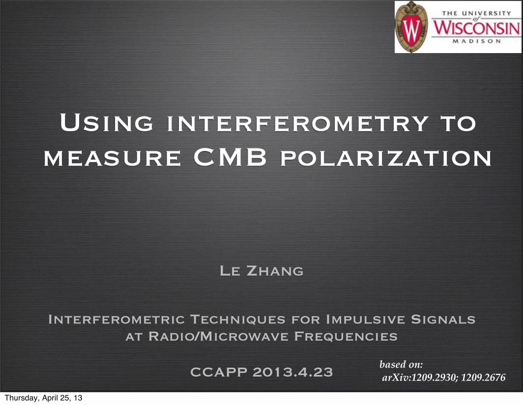
What the simulator can do?

Simulate CMB Stokes fields I,Q,U

Simulate interferometric CMB observations to generate mock visibilities (instrumental noise, beam pattern, uv-coverage, systematics)

Use two techniques Gibbs sampling(GS)/maximum likelihood(ML) to recover the underlying power spectra

Provide optimal sky map reconstruction

Simulation can test the ability of our instruments in CMB power spectrum recovery:


5

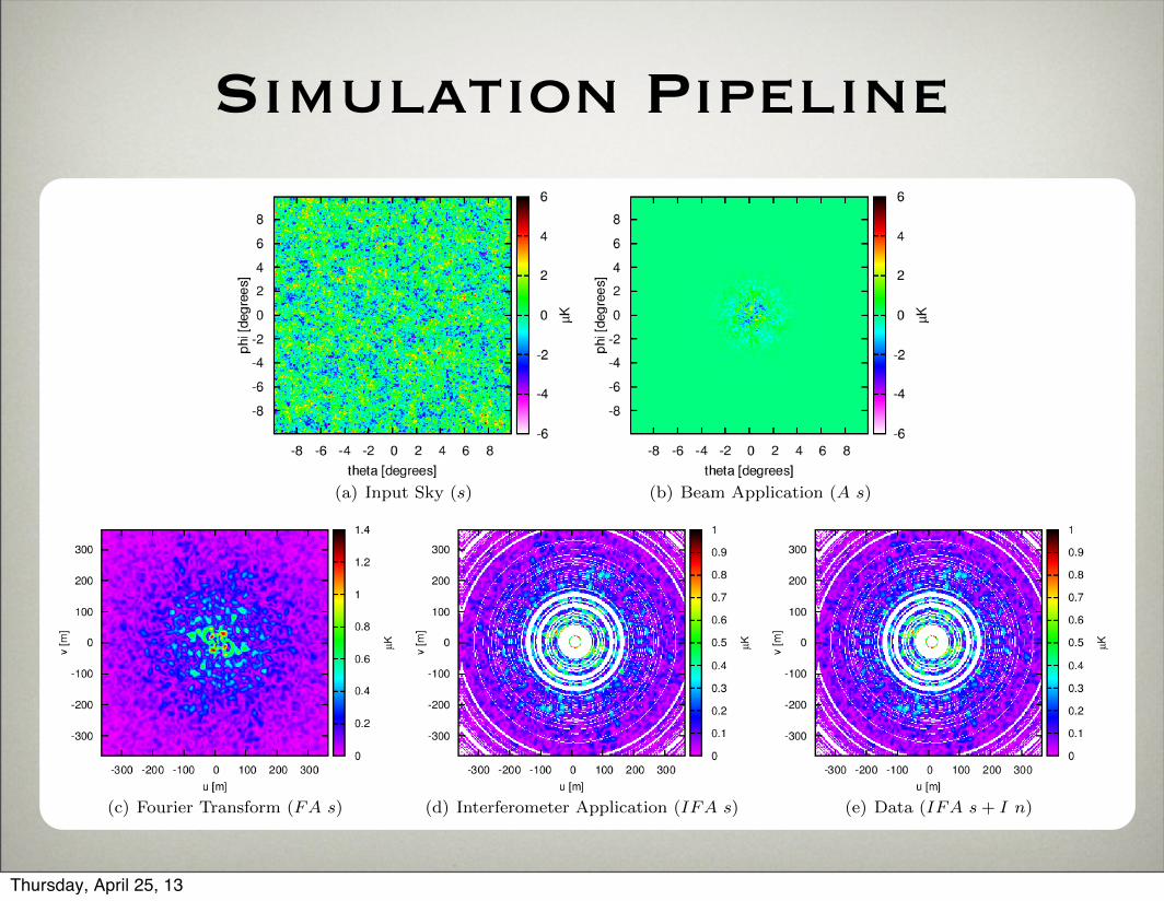
(a) Input Sky (s) (b) Beam Application (A s)

(c) Fourier Transform (FA s) (d) Interferometer Application (IFA s) (e) Data (IFA s+ I n)

Fig. 3.— Observation-making process. Shown are (a) the input sky signal s, (b) the application of a primary beam, which we model asa Gaussian with standard deviation 1.5 deg, (c) Fourier transformation onto the uv-plane, (d) application of 20 randomly placed antennasrotated uniformly for 12 hr, and (e) the addition of the noise. Note that all images in the uv-plane are shown as magnitudes.

of the example analysis we present here; however, theywould be more important in the limit where detectornoise is large compared to the observed signal (e.g., if thegoal was to place upper limits on an as-yet unobservedsignal, as is currently the case with inflationary B-modemissions). This issue will therefore have to be revisitedfor polarization data. In any case, if long correlationlengths in the Markov chain were to cause poor perfor-mance, we could follow the general prescription of Jewellet al. (2009) by incorporating a step with a Metropolis-Hastings sampler and deterministic rescaling of the skysignal.

4. RESULTS

4.1. Power Spectrum

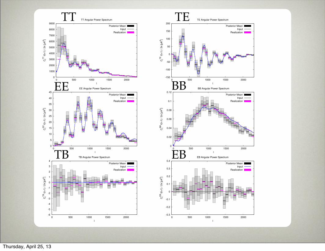
In Figure 5 we show the mean posterior angular powerspectrum of the of the four independent chains afterreaching convergence. We also show the uncertainty as-sociated with each `-bin and the corresponding power ofour input signal realization. The size of the uncertaintiesin each bin are consistent with varying coverage in theuv-plane; i.e., those bins with little to no coverage havecorrespondingly large error bars, while those bins withcomplete coverage have the tightest constraints. All ofour estimates fall within 2� of the expected value, andmost within 1�, as expected with this number of bins.Figure 6 shows individual marginalized probability

densities for a selection of `-bin. We immediately notethe shape of each probability distribution matches qual-itatively that of an inverse gamma distribution, as ex-pected. We see the damaging e↵ects of the lack of uv-

0

50

100

150

200

250

300

350

400

450

500

550

0 0.2 0.4 0.6 0.8 1

Num

bers

of S

teps

Until

Conve

rgence

Percent Covered

Fig. 4.— Number of steps after burn-in required to satisfy theG-R convergence criterion versus the sky coverage percentage foreach `-bin.

plane coverage especially in the case of ` ⇠ 300. Here, thelack of any input signal leads to a uniformly decreasingposterior probability density function (pdf) with a verylong power-law tail to large power. This can be summa-rized as an upper bound on the power in that bin. Inother bins, slightly reduced coverage combined with thee↵ects of noise yields wide and noisy distributions.Beyond the marginalized posteriors for each angular

power spectrum bin amplitude, the posterior samplesalso contain higher-order information. Figure 7 showsthe two-point correlations between all pairs of angularpower spectrum bins. For this plot, we suppress the di-

Simulation Pipeline


4

power spectra are listed in Table 1. In the flat sky ap-proximation, the 2D power spectrum 4!2|u|2S(|u|) !"("+ 1)C!|!=2"u for " ! 10 (White et al. 1999).

2.2. Simulated Observations

The CMB Stokes fields are believed to be isotropicand Gaussian in the standard inflationary models (Guth1981; Kamionkowski et al. 1997a,b; Zaldarriaga & Sel-jak 1997). On a small patch of the sky, the correspond-ing Fourier components of these fields are complex ran-dom variables and the value of the real and imaginaryparts of each point u in Fourier space are drawn inde-pendently from a normal distribution with zero meanand variance " C!|!=2"|u|. With cosmological parame-ters derived from WMAP 7-year results (Larson et al.2011; Komatsu et al. 2011), we use the public codeCAMB (Lewis et al. 2000) to compute the CMB powerspectra CTT

! , CEE! , CTE

! , CBB! . The input B-mode con-

tains a primordial component with a tensor-to-scalar per-turbation ratio, r, and a secondary component inducedby lensing. In our simulation we fix r = 0.01, the goalfor many current observations.Based on these power spectra, we generate Fourier

modes and then perform the inverse Fourier transformto obtain real-space Stokes fields I(x), Q(x) and U(x).From Eq. 5, for a given Jones matrix and beam responseG, the Stokes visibilities are then obtained by performingthe Fourier transform again.We assume the instrumental noise at each point of

the uv-plane is a complex, Gaussian-distributed numberwhich is independent between di!erent baselines (Whiteet al. 1999; Morales & Wyithe 2010). For an instrumentwhich measures both polarizations with an identical un-certainty in Stokes parameters, we can separately gener-ate the Gaussian noise with identical rms levels for eachI, Q and U visibility. The correlation function of thenoise for baselines i and j is determined by

CijN =

!

#2Tsys

$AAD

"2 !1

"#tanb

"

%ij , (15)

where Tsys stands for the system noise temperature, #for the observing wavelength, AD for the physical areaof a antenna, $A for the aperture e#ciency, "# for band-width, nb for the number of baselines with the same base-line vector u and ta for the integration time of the base-line.In order to illustrate the e!ect of systematic errors on

the recovered CMB power spectra and set allowable tol-erance levels for those errors, we perform simulations fora specific interferometer design. We choose an antennaconfiguration similar to that of the QUBIC instrument(Battistelli et al. 2011) which is under construction forobservations at 150 GHz. In our simulation, the interfer-ometer is a two-dimensional square close-packed array of400 horn antennas with Gaussian beams of width 5! inthe intensity beam pattern A(x), corresponding to# 7.1!

in G(x). The antennas have uniform physical separationsof 7.89#. With this configuration, the resolution in theuv-plane is about &u = 1.82 ("" ! 11), and the uv cov-erage reaches down to " ! 50 $ 2"" = 28, probing theprimordial B-mode bump at " % 50.We also assume that all Stokes visibilities. I, Q and

U , can be measured simultaneously for each antenna pair

with an associated rms noise level of 0.015µK per visi-bility, roughly corresponding to low-noise detectors eachwith 150µKs1/2 and a total integration time of threeyears. With this noise level, the simulations show thatthe averaged overall signal-to-noise ratio (SNR) in StokesQ and U maps is about 5. The high SNR ensures an accu-rate recovery of the B-mode power spectrum and allowsus to see systematic e!ects clearly.We generate realizations of Stokes parameter maps

having a physical size of 30 degrees on a side and resolu-tion of 64& 64 pixels. This large patch size ensures thatthe intensity beam pattern |G|2 at the edges decreases to# 1-percent level of its peak value. Although this size ofpatch seems to severely violate the flat-sky approxima-tion, the primary beam pattern itself is small enough (thefield-of-view $ is about 0.047 sr) so that the flat-sky ap-proximation is still valid. For simplicity, we assume thatall the antennas continuously observe the same sky patchat a celestial pole and the interferometer is located at thenorth or south pole , the uv-tracks should be perfectlycircular for a 12-h observation. Fig. 2.2 shows the mocksystematics-free visibility data from these observations.

3. MAXIMUM LIKELIHOOD ANALYSIS

The maximum likelihood estimator of the power spec-trum has many desirable properties (Bond et al. 1998;Kendall et al. 1987). The idea is to choose a model forthe data and construct a likelihood estimator to evaluatehow well the model matches the data. For a given model,comparing to the actual data set will give a likelihood ofthe model parameters. In practice, it is easier to max-imize the logarithm of the likelihood function than thelikelihood function itself.Since CMB Stokes visibilities are complex Gaussian

random variables with zero mean and dispersion CV +CN , the logarithm of the likelihood function is given by

lnL(C!) = n log !$ log |CV +CN |$V†(CV +CN )"1

V ,(16)

where V is the visibility data vector, CV is the signal co-variance matrix predicted by 'V†V(, which can be con-structed through Eq. 14, and CN is the noise covariancematrix, which can be computed by Eq. 15.In practice, we parameterize the CMB power spectrum

C! as flat band-powers over some multipole range toevaluate the likelihood function (Bunn & White 1996;Bond et al. 1998; Gorski et al. 1996; White et al.1999). We divide the power spectrum "(" + 1)C! intoNb piecewise-constant bins. Each bin corresponds toseparate annuli in the uv-plane, characterizing the av-eraged C! over its bin-width. In our case, we evaluatethe likelihood function by varying the CMB band-powers{CTT

b , CEEb , CBB

b , CTEb , CTB

b , CEBb } with b = 1, . . . , Nb.

Here Cb ) 2!|ub|2S(|ub|).The bin-width can be chosen arbitrarily, but an ap-

propriate choice of width is fine enough resolution toaccurately detect the structure of the power spectrumand also wide enough to reduce the correlation betweenthe band-power estimates so that the statistical errorson di!erent band-power bins are approximately uncor-related. The natural choice of bin-width can be ap-proximated by the characteristic width of the Fouriertransformed intensity beam pattern A(x), which definesthe typical correlation length in the uv-plane. The

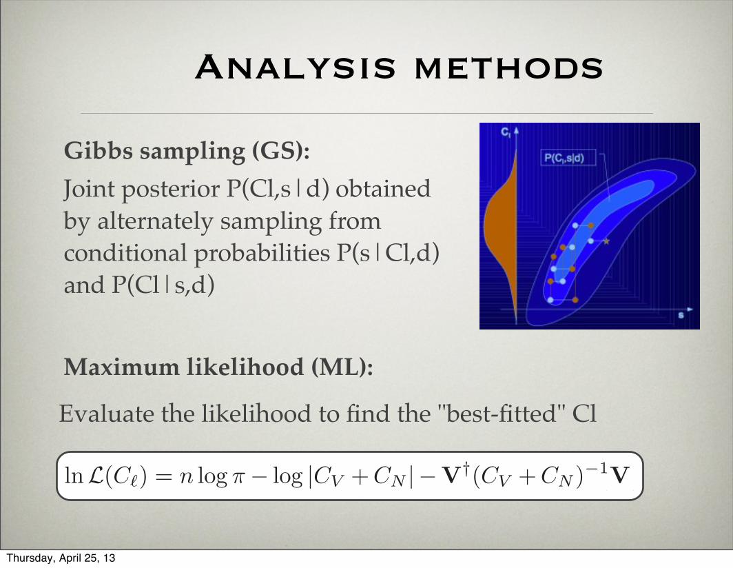
Maximum likelihood (ML):

Evaluate the likelihood to find the "best-fitted" Cl

Gibbs sampling (GS): Joint posterior P(Cl,s|d) obtained by alternately sampling from conditional probabilities P(s|Cl,d) and P(Cl|s,d)

Analysis methods


5

0

1000

2000

3000

4000

5000

6000

7000

8000

9000

0 500 1000 1500 2000

ClT

T l(

l+1)

/ 2

! [

µK

2]

l

TT Angular Power Spectrum

Posterior Mean

Input

Realization

-150

-100

-50

0

50

100

150

200

0 500 1000 1500 2000

ClT

E l(

l+1)

/ 2

! [

µK

2]

l

TE Angular Power Spectrum

Posterior Mean

Input

Realization

0

5

10

15

20

25

30

35

40

45

0 500 1000 1500 2000

ClE

E l(

l+1)

/ 2

! [

µK

2]

l

EE Angular Power Spectrum

Posterior Mean

Input

Realization

0

0.02

0.04

0.06

0.08

0.1

0.12

0 500 1000 1500 2000

ClB

B l(

l+1)

/ 2

! [

µK

2]

l

BB Angular Power Spectrum

Posterior Mean

Input

Realization

-6

-5

-4

-3

-2

-1

0

1

2

3

4

0 500 1000 1500 2000

ClT

B l(

l+1)

/ 2

! [

µK

2]

l

TB Angular Power Spectrum

Posterior Mean

Input

Realization

-0.3

-0.2

-0.1

0

0.1

0.2

0.3

0.4

0 500 1000 1500 2000

ClE

B l(

l+1)

/ 2

! [

µK

2]

l

EB Angular Power Spectrum

Posterior Mean

Input

Realization

Figure 4. Mean posterior power spectra for each `-bin are shown in black. Dark and light grey indicate 1� and 2� uncertainties,respectively. The binned power spectra of signal realization are shown in pink. Blue lines are the input CMB power spectra obtained byCAMB for a tensor-to-scalar ratio of T/S = 0.01.

Figure 5. Correlation matrices of TE, EE and BB power spectra � only the o↵-diagonal elements are shown. Correlations and anti-correlations between nearby power spectrum bins are the results of having a finite beam width and a finite bin size, respectively. Correlationsare stronger towards lower signal-to-noise values (from TE to BB) and towards higher `-values.

TT TE

EE

TB

BB

EB


I

Q

U

Real signals Recovered Dirty 30GHz 7

(a) Signal Realization (c) Final Mean Posterior Map (c) Dirty Map

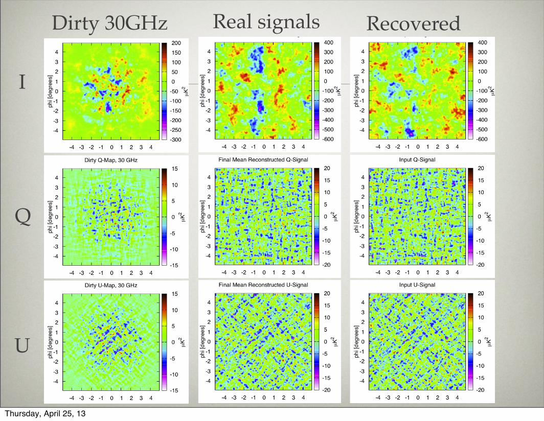
Figure 8. Signal maps. a) The signal realization, which is constructed from the input power spectra shown in blue in Figure 4, isused as the input map for the interferometer simulation. b) The final mean posterior map is the sum of solutions of Eq. 7 and Eq. 8;⌦F

�1R(~x+ ~y)↵, transformed into Stokes variables T , Q and U and averaged over all iterations. It provides the reconstruction of the

noiseless input signal by the Gibbs sampler within the area of the primary beam. c) The dirty map is simply the inverse Fourier transformof the data. The three rows show, from top to bottom, temperature, Stokes Q and Stokes U parameters.

duced as patches cut out from full-sky maps, then the“realization” and the “mean posterior” power spectra inFigure 4 would have been severely contaminated by E-B coupling, which can be easily resolved in the flat-skyapproximation (Bunn 2002).Our Gibbs sampling approach is also applicable to

more realistic cases of interferometic polarimetry simula-tions, such as close-packed arrays with systematic errors.Such simulations with varying systematics can providean idea about the limitations of interferometers for up-coming missions, such as the QUBIC experiment, whichaims to detect B-mode polarization anisotropies of theCMB signal.

ACKNOWLEDGMENTS

Computing resources were provided by the Universityof Richmond under NSF Grant 0922748. Our implemen-tation of the Gibbs sampling algorithm uses the open-source PETSc library (Balay et al. 1997, 2010, 2011)and FFTW (Frigo & Johnson 2005). G. S. Tucker andA. Karakci acknowledge support from NSF Grant AST-

0908844. P. M. Sutter and B. D. Wandelt acknowledgesupport from NSF Grant AST-0908902. B. D. Wandeltacknowledges funding from an ANR Chaire d’Excellence,the UPMC Chaire Internationale in Theoretical Cosmol-ogy, and NSF grants AST-0908902 and AST-0708849.L. Zhang and P. Timbie acknowledge support from NSFGrant AST-0908900. E. F. Bunn acknowledges sup-port from NSF Grant AST-0908900. We are grateful forthe generous hospitality of The Ohio State University’sCenter for Cosmology and Astro-Particle Physics, whichhosted a workshop during which some of these resultswere obtained.

REFERENCES

Balay, S., Gropp, W. D., McInnes, L. C., & Smith, B. F. 1997, inModern Software Tools in Scientific Computing, ed. E. Arge, -Revision 3.1, Argonne National Laboratory A. M. Bruaset, &H. P. Langtangen, (Birkhauser Press) 163 202.

Balay, S., Gropp, W. D., McInnes, L. C., & Smith, B. F. 2010,PETSc Users Manual - Revision 3.1, Argonne NationalLaboratory - http://www.mcs.anl.gov/petsc/

7







ACKNOWLEDGMENTS



REFERENCES



7







ACKNOWLEDGMENTS



REFERENCES




Documents

Using interferometry to measure CMB polarization - …ccapp.osu.edu/workshops/RadioSim2/talks/08-le-zhang-cmb-ohio.pdf · Using interferometry to measure CMB polarization ... provided