Using global arrays to investigate internal-waves and mixing

Jennifer MacKinnon,1 Matthew Alford,2 Pascale Bouruet-Aubertot,3 Nathan Bindoff,4 Shane Elipot,5 Sarah Gille,6 JamesGirton,7 Mike Gregg,8 Robert Hallberg,9 Eric Kunze,10 Alberto Naveira Garabato,11 Helen Phillips,12 Rob Pinkel,13 Kurt

Polzin,14 Tom Sanford,15 Harper Simmons,16 Kevin Speer17

1 Corresponding author, Scripps Institution of Oceanography, USA, jmackinn@ucsd.edu2 University of Washington, USA, malford@apl.washington.edu

3 LOCEAN/IPSL, France, Pascale.Bouruet-Aubertot@locean-ipsl.upmc.fr4 University of Tasmania, Australia, n.bindoff@utas.edu.au

5 Proudman Oceanographic Laboratory, UK, ship@pol.ac.uk6 Scripps Institution of Oceanography, USA, sgille@ucsd.edu7 University of Washington, USA, girton@apl.washington.edu8 University of Washington, USA, gregg@apl.washington.edu

9 Geophysical Fluid Dynamics Laboratory, USA, Robert.Hallberg@noaa.gov10 University of Victoria, Canada, kunze@uvic.ca

11 National Oceanographic Center, UK, acng@noc.soton.ac.uk12 University of Tasmania, Australia, h.e.phillips@utas.edu.au

13 Scripps Institution of Oceanography, USA, rpinkel@ucsd.edu14 Woods Hole Oceanographic Institution, USA, kpolzin@whoi.edu

15 University of Washington, USA, sanford@apl.washington.edu16 University of Alaska, USA, hsimmons@sfos.uaf.edu

17 Florida State University, USA, kspeer@ocean.fsu.edu

Abstract

Turbulent diapycnal mixing in the ocean controls the transport of heat, freshwater, dissolved gases, nutrients, andpollutants. Though many present generation climate models represent turbulent mixing with a simplistic diffusivity be-low the surface mixed layer, the last two decades of ocean mixing research have instead revealed dramatic spatial andtemporal heterogeneity in ocean mixing. Climate models that do not appropriately represent the turbulent fluxes of heat,momentum, and CO2 across critical interfaces will not accurately represent the ocean’s role in present or future climate.An accurate picture of the worldwide geography of mixing requires a vastly increased database of observations. Unfor-tunately, traditional microstructure estimates of turbulent mixing are expensive, difficult, and rare. A key development ofthe last decade has been the development of tools to estimate the turbulent mixing rate from finescale (order 10-50 meterresolution) measurements of internal-wave shear and vertical strain. Global arrays such as the Argo program providean unprecedented and as yet underdeveloped opportunity to define the global internal wave climate, and in turn identifymixing patterns and hotspots.

1 INTRODUCTION

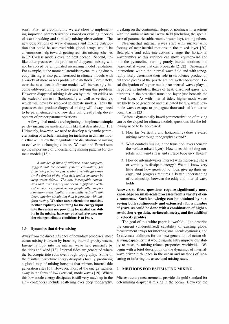
The clearest conclusion to emerge from the last severaldecades of ocean mixing research has been the dramaticpatchiness of turbulence in the ocean. For example, Fig.1 shows depth-averaged turbulent dissipation rate as esti-mated from fine-scale shear/strain (Section 2.2 below) fromthe World Ocean Circulation Experiment data. Both the dis-sipation rate (left panel) and diffusivity (right panel) varyby several orders of magnitude across any given oceanbasin. Two patterns visible in this figure are emblematic ofglobal mixing patterns, namely 1) mixing is elevated overrough topography (e.g. where the line crosses the SW In-dian Ridge) and 2) turbulent diffusivity often increases withdepth.

1.1 The importance of patchy mixing

Observing and understanding the global geography of tur-bulent mixing is crucial for several reasons. First, with-

out adequate global sampling we cannot accurately knowthe average turbulent diffusivity or buoyancy flux at anygiven depth, or basin-wide. One of the driving ques-tions in small-scale physical oceanography over the lastdecades has been the perceived order of magnitude differ-ence between the 10−4 m2 s−1 average diffusivity requiredto power the meridional overturning circulation [3] and the10−5 m2 s−1 diffusivity most often observed [4]. Severalpossible resolutions to this discrepancy have been proposed,ranging from enhanced mixing over rough topography [5,6]to wind-driven isopycnal fluxes in the Southern Ocean [7].However, without significantly improved sampling den-sity we cannot compute accurate global averages of tur-bulent diffusivity.

Second, the details of mixing distribution can have se-vere consequences for modeled global circulation. Belowthe surface mixed layer, most current generation climatemodels employ a combination of a simple Richardson num-ber parameterization for diffusivity and a horizontally uni-

Figure 1: A typical example of vertical and lateral inhomogeneity of diapycnal diffusivity in the ocean: here diffusivity is inferredfrom WOCE Lowered ADCP data using a finescale parameterization along 32S in the Indian Ocean. White corresponds roughly to thediffusivity expected from wave breaking in a ’background’ Garrett-Munk level wavefield, as indicated on the colorbar. Fig. reproducedfrom [1, 2].

form background diffusivity profile. The former are cali-brated to (and necessary for) reasonable representation oflarge-scale sheared flows such as the equatorial undercur-rent or high-latitude dense water overflows [8]. However,they are only relevant for cases where the resolved Richard-son number leads to turbulent mixing. Climate models donot resolve the vertical scales of breaking internal waves(meters) and will not do so for the forseeable future, sothe present suite of Richardson number based parameteriza-tions do not represent the largest source of diapynal mixingin the open ocean. The addition of background diffusiv-ity profiles that generally increase with depth [9] is meantto crudely replicate the zonally averaged structure of turbu-lent mixing based on observations [1,10]. While better thana constant background diffusivity, simple diffusivity pro-files ignore the observed horizontal patchiness of mixing,which can have severe consequences for global circulationpatterns.

The nature of these consequences depend on the depth(or isopycnal) of diapycnal fluxes. Deep mixing controls theheat and carbon dioxide storage in the ocean and is impor-tant for evolution on long timescales. To understand the ef-fect of horizontally patchy mixing, consider the conceptualmodel of abyssal circulation given by Stommel and Arons.In the traditional view, uniform deep mixing provides a con-vergent downward turbulent buoyancy flux, with the up-welling rate across any given isopyncal surface roughlygiven by

A× w∗ =1N2

∂

∂z[κN2A] (1)

where A is the area of that isopycnal surface, N the buoy-ancy frequency, and κ(x, y, z) the diapycnal diffusivity.When the diapycnal diffusivity (κ) is assumed constant, thepositive buoyancy frequency gradient leads to convergent

buoyancy flux and upwelling, vortex stretching, and pole-ward flow. However, when diffusivity is bottom enhanced(Fig. 1), the bracketed term in (1) can be negative, pro-ducing local downwelling [11]. While the isopycnal areaterm, A, usually contributes in such a way that there is stillnet upwelling across each isopycnal surface, the pattern ofabyssal circulation can change dramatically if κ is laterallyinhomogeneous [11–13].

The geography of upper ocean mixing also has a sig-nificant impact on oceanic circulation, water properties andheat fluxes. For example, one of the most robust conclu-sions from two decades of research is that upper oceanmixing has a strong latitudinal dependence, with a steadydecline towards the equator, due indirectly to the chang-ing bandwidth of the the internal wave frequency spec-trum with changing latitude [14, 15]. This pattern of upperocean and thermocline mixing was recently implementedin a global coupled model [16]. They found significantlyreduced model biases, changes in equatorial stratification,and reduced heat uptake by the atmosphere compared tomodel runs with laterally uniform diffusivity. Observationsalso show episodically enhanced internal-wave driven mix-ing in the highly stratified transition zone beneath the sur-face mixed layer [17] that are not represented in currentmixed-layer parameterizations. Turbulent fluxes in this re-gion are crucial for mediating air-seat heat exchange andbiologically essential nutrient transport.

1.2 Modeling patchy mixing

Though diapycnal mixing is only one of many impor-tant processes crudely represented by climate models (e.g.,cloud physics, oceanic and atmospheric convection, effectsof sea-ice heterogeneity, etc.), it is noteworthy for two rea-

sons. First, as a community we are close to implement-ing improved parameterizations based on existing theoriesof wave breaking and (limited) mixing observations. Thenew observations of wave dynamics and mixing distribu-tion that could be achieved with global arrays would bean enormous help towards getting realistic mixing schemesin IPCC-class models over the next decade. Second, un-like other processes, the problem of diapycnal mixing willnot be solved by anticipated increasing model resolution.For example, at the moment lateral/isopycnal mixing due toeddy stirring is also parameterized in climate models witha variety of more or less problematic methods. Fortunately,over the next decade climate models will increasingly be-come eddy-resolving, in some sense solving this problem.However, diapycnal mixing is driven by turbulent eddies onthe scales of cm to m (horizontally as well as vertically),which will never be resolved in climate models. Thus theprocesses that produce diapycnal mixing will always needto be parameterized, and new data will greatly help devel-opment of proper parameterizations.

A few global models are beginning to implement simplepatchy mixing parameterizations like that described in [13].Ultimately, however, we need to develop a dynamic param-eterization of turbulent mixing for inclusion in climate mod-els that will allow the magnitude and distribution of mixingto evolve in a changing climate. Wunsch and Ferrari sumup the importance of understanding mixing patterns for cli-mate models [18]:

A number of lines of evidence, none complete,suggest that the oceanic general circulation, farfrom being a heat engine, is almost wholly governedby the forcing of the wind field and secondarily bydeep water tides... The now inescapable conclu-sion that, over most of the ocean, significant verti-cal mixing is confined to topographically complexboundary areas implies a potentially radically dif-ferent interior circulation than is possible with uni-form mixing. Whether ocean circulation models...neither explicitly accounting for the energy inputinto the system nor providing for spatial variabil-ity in the mixing, have any physical relevance un-der changed climate conditions is at issue.

1.3 Dynamics that drive mixing

Away from the direct influence of boundary processes, mostocean mixing is driven by breaking internal gravity waves.Energy is input into the internal wave field primarily bythe tides and wind [18]. Internal tides are generated wherethe barotropic tide rubs over rough topography. Some ofthe resultant baroclinic energy dissipates locally, producinga global map of mixing hotspots that mirrors internal tidegeneration sites [6]. However, most of the energy radiatesaway in the form of low (vertical) mode waves [19]. Wherethis low-mode energy dissipates is still very much up in theair - contenders include scattering over deep topography,

breaking on the continental slope, or nonlinear interactionswith the ambient internal wave field (including the specialcase of parametric subharmonic instability), among others.

Near-inertial internal waves start with surface windforcing of near-inertial motions in the mixed layer [20].Beta-plane and eddy-interactions change the horizontalwavenumber so this variance can move equatorward andinto the pycnocline, turning purely inertial motions intonear-inertial waves that can propagate [21, 22]. Subsequentinteractions within the internal wave field and with topog-raphy likely determine their role in turbulence productionbut these pieces of the puzzle are not well-understood. Lo-cal dissipation of higher-mode near-inertial waves plays alarge role in turbulent fluxes of heat, dissolved gases, andnutrients in the stratified transition layer just beneath themixed layer. As with internal tides, higher-mode wavesare likely to be generated and dissipated locally, while low-mode waves escape to propagate thousands of km acrossocean basins [23].

Before a dynamically based parameterization of mixingcan be developed for climate models, questions like the fol-lowing need to be addressed:

1. How far (vertically and horizontally) does elevatedmixing over rough topography extend?

2. What controls mixing in the transition layer (beneaththe surface mixed layer). How does this mixing cor-relate with wind stress and surface buoyancy fluxes?

3. How do internal-waves interact with mesoscale shearor vorticity to dissipate energy? We still know verylittle about how geostrophic flows give up their en-ergy, and progress requires a better understandingof relationships between the eddy and internal wavefields.

Answers to these questions require significantly moreknowledge on small-scale processes from a variety of en-vironments. Such knowledge can be obtained by sur-veying both continuously and extensively for a numberof years, as could be done with a combination of higher-resolution Argo data, surface altimetry, and the additionof velocity profiles

The goal of this white paper is twofold: 1) to describethe current (underutilized) capability of existing globalmeasurement arrays for inferring small-scale dynamics, and2) advocate additions for the next generation of ocean ob-serving capability that would significantly improve our abil-ity to measure mixing-related properties worldwide. Webegin with a brief description on the dynamics of internal-wave driven turbulence in the ocean and methods of mea-suring or inferring the associated mixing rates.

2 METHODS FOR ESTIMATING MIXING

Microstructure measurements provide the gold standard fordetermining diapycnal mixing in the ocean. However, the

instruments needed to carry out these measurements arecostly, and experienced teams are required to deploy and re-cover them. As a result, microstructure measurements havebeen conducted in only a limited number of geographic lo-cations across the globe. While it is essential that the com-munity continue to make these measurements, a variety ofcomplementary methods have emerged to approximate ver-tical diffusivities by taking advantage of finestructure mea-sured by instruments that are more readily available.

2.1 Turbulent overturns

The most direct way to measure turbulent mixing is to mea-sure the scales at which turbulent overturns are actually oc-curring. Turbulent diffusivity κ is related to the turbulentdissipation rate ε, which is easier to measure, through anassumed mixing efficiency

κ ∼ Γε

N2, (2)

where Γ is typically taken to be 0.2 [25, 26]. Since mostoceanographic measurements are in the form of verticalprofiles, the dimensions of turbulence are often discussedin terms of vertical scales (Fig. 2). Turbulence in stratifiedwater is bounded at the upper end by the Ozmidov scale,

L0 =2πm0

=√

ε

N3∼ O(0.1− 10 m), (3)

and at the lower end by the Kolmogorov scale (order ofmm). The latter is the scale at which viscosity actuallydiffuses momentum, while the former is related to outerscales of turbulent overturns. Traditional microstructure in-struments measure well into the inertial subrange betweenthese scales, and estimates of the turbulent dissipation rateare based on fits to assumed spectra of velocity or temper-ature fluctuations. This is an accurate but difficult and ex-pensive measurement to make. However, the outer scalesof turbulent overturns can often be measured with stan-dard CTD sensors, provided that the data are saved at ahigh enough resolution. The quantity typically calculatedis known as the Thorpe scale (Lt), defined as the root meansquared displacement a parcel has moved between a mea-sured density profile with a density inversion (overturn) andthe sorted version of the same profile. The Thorpe scalehas been shown to be a good estimate of the Ozmidov scale(Lt ∼ L0), so CTD measurements of density inversionscan be used to estimate ε through (3) [27–29]. The resultsgenerally compare well with microstructure estimates (e.g.[29–31], Fig. 3). The largest drawback of this method is theaccuracy required to measure density overturns at scales ofmeters or less. For low-level turbulence and weak stratifica-tion these scales are right up against the noise level of mostCTDs. However, in energetic regimes turbulence may pro-duce overturns of tens of meters or more, which should bedetectable by a wide variety of platforms.

2.2 Finescale parameterizations of mixing

Over the last few decades, a variety of empirical, statisti-cal, and theoretical models have been developed to relatefinescale (tens to hundreds of meters vertically) shear andstrain from internal waves to the associated turbulent dis-sipation rate and diffusivity. The basic idea is that weaklynonlinear interactions between a well-developed sea of in-ternal waves act to steadily transport energy from the large(vertical) scales at which it is generated and propagates,to the small scales at which waves break due to shear orconvective instabilities. The more energetic the wavefield,the faster this rate of down-scale transfer and the larger thedissipation rate and associated diffusivity [33, 34]. Morespecifically, internal wave shear and strain tend to have flatvertical wavenumber spectra at scales larger than about 10m (mk in the left panel of Fig. 2). The rate of downscaleenergy transfer through these scales (and thus the dissipa-tion rate) tends to scale quadratically with the spectral levelE,

ε ∼ E2, (4)

a scaling consistent between theory [14], observations [15,24, 35] (Fig. 2), and numerical simulations [36].

The ability to infer turbulent dissipation rates fromfinescale quantities has profound implications for develop-ing global estimates of mixing rate. Wijesekera et al. statethe case well [37]:

...If [predicting the dissipation rate based on in-ternal wave dynamics] is even approximately true,the significant oceanographic problem of estimatingvertical viscosities and diffusivities for large-scalemodeling applications shifts from adequately sam-pling the processes responsible for mixing to defin-ing the global internal wave climate.

The Gregg-Henyey-Polzin method, as it is sometimesknown, does not work in all environments. In particular, itassumes dissipation is produced by weakly nonlinear inter-actions in a broadband field of internal waves. The scalingfails where internal waves are strongly nonlinear (e.g. soli-tons), in shallow water where the internal wave field has amuch reduced vertical bandwidth [38, 39], or where large-scale baroclinic motions are directly breaking. For exam-ple, [31] find the G-H-P scaling to be over an order of mag-nitude too small right above the Hawaiian Ridge, where alarge-amplitude internal tide is directly breaking, but agreequite well with microstructure estimates only hundreds ofmeters away (Fig. 3). Even in the best environments, uncer-tainties remain as to the error bars associated with this tech-nique. Ongoing detailed comparison between microstruc-ture and finescale parameterizations by a number of inves-tigators should help.

vertical wavenumber

Nor

mal

ized

she

ar v

aria

nce

!s /

N2

m"mOmk

quasi-linear internal waves

strongly nonlinear

regime

Dissipation (#)

wave-wave interactions

Shea

r sp

ectr

al d

ensi

ty (

s-2 /

cpm

)In

ferr

ed D

iffus

ivity

( m

2 /s)

Vertical Wavenumber (cpm)

Diffusivity Parameterization (m2/s)

Ê

Saturday, October 10, 2009

Figure 2: Left: Sketch of idealized vertical wavenumber spectra of stratification normalized shear showing steady-state spectralshapes for the internal wave regime (low wavenumbers / large vertical scales), the transition range, and the turbulent subrange at highwavenumbers / small vertical scales. Wavenumbers indicated on the x-axis correspond to the Kolmogorov scale (mν ), the Ozmidovscale (mO), and the edge of the quasi-linear internal wave regime (mk). The blue arrows schematically indicate the direction of energytransfer from large to dissipative scales. Right: Demonstration of shear spectral shape and Gregg-Henyey-Polzin dissipation rate scal-ing, from [24]: Shear spectra scaled in the vertical by 1/E1N

2 and in the horizontal by E1 for a variety of data sets (top); diffusivitiesinferred from microstructure measurements plotted against a fine-scale parameterization showing good agreement (bottom).

3 ESTIMATING MIXING FROM GLOBAL AR-RAYS

Global arrays such as the Argo program provide an unprece-dented opportunity to improve our knowledge of finescaleprocesses in the ocean. The sheer quantity of data andglobal coverage represent a huge addition to ship-basedmeasurements. Perhaps their greatest potential is in sam-pling small-scale processes in inaccessible or inhospitablelocations and times, such as the Southern Ocean or beneathwinter storms. Such environments are challenging for ship-based observations, yet are likely to be hotspots of turbulentmixing. Below we discuss the potential for measurementof small-scale process from existing instruments and arguefor improvements in the next generation of measurements.This is not intended to be a comprehensive list of availabledata or analysis possibilities, but rather a starting point forongoing discussion.

3.1 Using existing measurements

Applying finescale parameterizations of turbulent dissipa-tion to current global ocean observing system data can dra-matically improve global estimates of mixing. The turbu-lent dissipation rate may be estimated by measuring either

shear or strain from internal waves at these scales [37], al-though the most accurate estimates require a combinationof the two [1]. In addition to the study pictured in Fig. 1,several other investigators have already applied this methodto Lowered ADCP data [40–43]. The strong and bottom-enhanced diffusivity calculated by [44] using this methodnear Drake Passage was a pivotal motivation for the ongo-ing multinational DIMES (Diapycnal and Isopycnal Mix-ing Experiment in the Southern Ocean) project. On theother hand, significant uncertainties remain, and care mustbe taken when interpreting method parameters and sensornoise.

Argo: Standard Argo floats make use of the ARGOStransmission system and are able to transmit a limited num-ber of data points per profile. Typically they attain verti-cal resolutions of 5 to 10 m in the upper ocean and 50 min the deep ocean. In most cases, this vertical resolutionis unlikely to be sufficient to infer any information aboutfinestructure mixing. However, Argo floats that make use ofthe Iridium communications system are able to send moredata, and some already provide profiles that may be suffi-cient for finestructure calculations. Moreover, if the Argoarray is transitioned to make use of Iridium (or any othersatellite communication system that allows higher volumes

Figure 3: A comparison of several methods for calculating the turbulent dissipation rate, ε, normalized by mean stratification (tomake a diapycnal diffusivity) for four time periods near Oahu. Data were taken during the Hawaiian Ocean Mixing Experiment andare reproduced from [31]. In each panel the thick black line is the estimate from the microconductivity probe; thin shaded line is fromdensity overturns; thick shaded line is from GreggHenyey parameterization. There was no microconductivity from the upper CTD forthe second two time periods. The dashed line is the composite dissipation profile from direct turbulence measurements made in deepwater atop the ridge [32].

of data to be sent) then higher vertical resolution could beachieved for the entire array. Though CTD data can be con-taminated by ship roll, Argo floats rise freely through thewater column and are unaffected by this. Thus they havethe potential to provide high-quality profiles well suited forfinestructure calculations. There is no clear cutoff to in-dicate what vertical resolution must be achieved to makeArgo floats useful for finestructure calculations, but we ex-pect that for most regions with typical background stratifi-cation, 1 to 2 m resolution data would be usable.

Ship based measurements: In addition to finescale es-timates of mixing from lowered ADCP data, Thorpe scalescan be calculated from standard shipboard CTDs, providedsome care is taken to understand relevant noise levels andthe contaminating effect of ship motion [45, 46]. Thorpescales can also be calculated from expendable CTDs, whichdo not have the problem of ship motion. XCTDs are reg-ularly deployed along repeat measurement lines, such asWOCE transect AX22 in the Drake Passage [47].

Mooring arrays: Long-term mooring collections suchas the RAPID array involve ADCPs, moored profilers, and

thermistor chains that may be used for finescale estimatesof mixing. Even where resolution is not high enough to ob-serve breaking waves, long term information on the internalwave climate in the deep ocean is an important part of theglobal energetics.

3.2 New tools and measurement strategies

One of the most straightforward improvements to globalmeasurements would come from consistently archivinghigh-resolution CTD data. In order for Thorpe scales orfine-scale strain to be calculated from shipboard CTD data,the data must be archived and made available at the high-est possible resolution (raw). Standard processing into 1-2dbar bins is not adequate. Even when features of interest(overturns) are several meters tall or more, careful post-processing in order to remove ship roll and salinity spikes isrequired to have the accuracy necessary to confirm densityinversions [46]. This processing is only possible if PIs haveaccess to the raw data.

Global finescale measurements from the Argo array

Time along float trajectory

Pre

ssure

[dbar

]To

pogr

aphy

[m

]

Friday, October 9, 2009

Figure 4: Examples of EM-APEX float measurements. Left: Thorpe scales calculated from an EM-APEX float, vertical resolutionapproximately 2 dbar, deployed at the northern Kerguelen Plateau (see inset map). Each line corresponds to a float profile and eachspike on the profiles matches a turbulent patch where the horizontal length of the spike (in the plot) represents the vertical Thorpescale for a particular overturning patch, Lt. The inset map also shows the local topography and the position of the northern, middleand southern Subantarctic Front (SAFN, SAFM, and SAFS respectively). [ Unpublished results from Ph.D. research of Amlie Meyer,University of Tasmania, Australia.] Right: (upper) Zonal velocity and (lower) Reduced shear (S2 − 4N2) from an EM-APEX floatin the 2007 CLIMODE experiment in the Gulf Stream. The velocity measurement shows both the along-stream velocity evolution andhigh-frequency variability due to internal waves (primarily storm-driven near-inertial waves). The reduced shear (a quantity that ispositive when the Richardson number is below 1/4 and the flow is susceptable to Kelvin-Helmholtz instability) indicates the most likelyregions to undergo mixing. Black lines are density contours in 0.1 kg/m3 intervals, and 17◦ and 19◦ isotherms are in magenta

would be significantly enhanced by three primary changes:

• Improved vertical resolution. Higher vertical sam-pling would not only allow far more accurate esti-mates of internal wave strain, but in some environ-ments would allow direct observation of turbulentoverturns. For example, Meyer and Phillips (Fig. 4,left) are able to calculate Thorpe scales (Sec. 2.1)in the energetic Kerguelan Plateau region. Thoughthey are using EM-APEX floats, similar calculationscould be done with any of the Argo array providedthe vertical resolution was high enough. Increas-ing the vertical resolution requires a financial com-mitment to the bandwidth required to send higherdensity data. An Argo array with enhanced resolu-tion would also allow us to resolve lateral (isopyc-nal) stirring processes and the higher modal struc-tures of mesoscale eddies (higher than mode one) thatare key to determining and understanding the controlsof eddy mixing rates.

• Deeper measurements. Turbulent diffusivity is of-ten bottom enhanced (Fig. 1), especially over roughtopography. Extension of the Argo array to includemeasurements below 2000 meters would make an in-valuable improvement towards our understanding ofdeep mixing in the worlds oceans. We emphasize thatmixing is elevated for hundreds of meters over roughtopography, so the profile would not need to be close

to the bottom to sample more regions of enhancedmixing. Argo floats are calibrated before launch butare not recovered for post-measurement calibration.For climate research this can pose a challenge, par-ticularly in the deep ocean where horizontal temper-ature gradients are small, since temporal evolutionof temperature or salinity may be difficult to distin-guish from instrument drift. However, finestructuremeasurements are not subject to calibration difficul-ties since they depend only on the vertical gradientsmeasured within a single profile.

• Adding velocity measurements. The new EM-APEXplatform (described in more detail below) adds hori-zontal velocity to the standard Argo package at abouta 60% increase in float cost (which could potentiallycome down to 20-30% with sufficient volume). In ad-dition to the many other applications of velocity pro-files, the information gained about the internal wavefield is a significant improvement over what is possi-ble with CTD (strain) alone. The shear-to-strain ra-tio of internal waves depends on their frequency andwavelength, as well as the environmental parametersof latitude and stratification, so strain alone can missimportant details of internal wave generation as wellas the scaling of dissipation.

EM-APEX floats - capability, strategies, examples.A new variant of the standard Webb Research APEX

profiling float used in Argo is now available with a subsys-tem for measuring motionally induced electric fields gener-ated by the ocean currents moving through the vertical com-ponent of the Earth’s magnetic field. Since this is a moresignificant change than other proposed array enhancements,we include some technical detail here. Electrodes on theupper end cap, below the SBE-41 CTD, sense the motion-ally induced voltages. The voltages are amplified, digitized,processed into velocity components and stored within thefloat. Other measurements are components of the Earth’smagnetic field (i.e., compass) and instrument tilt. Float po-sition is determined by the global positioning system whenthe float surfaces. The T, S, V, position, and other observa-tions are processed within the float and transmitted over theIridium global cell phone system. The Iridium link is bi-directional, allowing not only data uploads but also down-loads of mission changes.

The horizontal electric field as observed on a platformmoving with the surrounding water is

∇hφa = −Fz(v − v∗)× k− J∗/σ, (5)

where φa is the apparent potential around a moving sen-sor (N.B. after correction is applied for the distortion of theelectric currents around the APEX float), Fz is the verticalcomponent of the Earth’s magnetic field, σ is electrical con-ductivity, v(z) is local water velocity, v∗ is a vertically inte-grated, conductivity weighted ocean velocity, and J∗ repre-sents non-local electric currents (typically negligible). Theimportant point is that only one term varies with depth. Itis this term that provides the vertical distribution of current.The other terms represent an unknown (but knowable withan independent velocity measurement, such as of the sur-face velocity from GPS observations), depth-independentoffset. As the profiler falls/rises at 0.1-0.12 ms−1 and ro-tates slowly, the electric field is measured every 1-s and fit-ted over 50 s to sine and cosine components derived fromthe magnetic sensor. This yields a velocity value every 5-6m. The fit is moved 25 s and repeated. Thus, velocity val-ues are computed every 2.5-3 m in the vertical. With alka-line batteries, the instrument should provide 150 profiles to2000 dbar. Lithium batteries will provide many more pro-files. EM-APEX equipped with Lithium batteries, deployednorth of the Kerguelen Plateau in the SOFINE experiment,have recorded in excess of 300 profiles to 1600 dbar and arestill operating.

EM-APEX floats have so far been deployed in fo-cused process experiments, including CBLAST, EDDIES,CLIMODE, PhilEx, SOFINE, and DIMES, and are compo-nents of several upcoming experiments, such as ITOP (ty-phoon) and LatMix ONR projects. Fig. 4 shows an exampleof velocity and shear measurements from the Gulf Stream(CLIMODE). [48] and [49] used EM-APEX profiles fromthe first deployment, in Hurricane Frances in 2004, to mea-sure the momentum flux into the ocean (used to derive newvalues of drag coefficient), SML cooling, and surface grav-ity wave amplitudes. In addition, the data provided valuable

information for numerical modeling of the ocean responsesto high wind stress events, such as tropical cyclones.

Novel profiling strategies can significantly help our un-derstanding of the internal wave climate. For example, con-ducting pairs of vertical profiles separated by half an iner-tial period allows easy identification of near-inertial shear.Fig. 5 shows subsurface near-inertial energy obtained from2 months of data from 3 EM-APEX floats in the SouthernOcean. By differencing profiles separated by 1/2 inertialperiod (about 7 hours at this latitude) a clear picture of thedownward propagation of near-inertial energy emerges.

3.3 Surface drifters and near-inertial oscillations

The global surface drifter array is an excellent tool for ob-serving near-inertial oscillations in the surface ocean, es-pecially in combination with suggested EM-APEX floatsto observe sub-surface evolution into near-inertial internalwaves. Due to large spatial and seasonal variability, it isdifficult to design ship-based observational programs to ob-serve near-inertial wave generation and evolution. How-ever, drifting global arrays provide an ideal platform, pro-vided that they sample at a high enough temporal resolutionto observe near-inertial motions. Until December 2004, thearray of surface drifters from the Global Drifter Programwas tracked by two Argos satellites resulting in 6 to 9 dailypositioning fixes at Equatorial latitudes to a theoretical 28fixes per at the poles [51]. From January 2005, NOAA ne-gotiated the use of the full Argos satellite constellation (5to 6 satellites). As a result, we have now achieved 16-20fixes per day at the equator and more towards higher lati-tudes. The global average for the time interval between twodrifter fixes is now 1.2 hours. As a result, oceanic variabil-ity at high frequencies, including near-inertial waves andsuper-inertial variability, is captured by surface drifter dis-placement, even in the high latitude ocean [52].

Several groups have already begun to take advantage ofthis resource for looking at high-frequency processes in theupper ocean. In a recent paper, [50] used surface driftervelocity data to compute a global seasonal climatology ofnear-inertial currents (Fig. 5) that confirmed and extendedthe earlier pioneer work of [53] who obtained characteris-tics of near-inertial motions on large scales based on thesurface drift of Argo floats. [50] compared their observa-tions of near-inertial energy to predictions by Pollard andMillard’s [1970] slab-layer model of near-inertial motionsand found great discrepency with the drifter observations.They therefore questioned the estimates of wind energy in-put to inertial motions based on this model. This suggeststhat estimates of wind energy input to inertial motions, po-tential energy for deep mixing, need to be re-evaluated. [54]find near-inertial oscillations are significantly modified bygeostrophic vorticity.

The GDP array currently comprises about 1250 driftersthat are managed by AOML. A complete understandingof the dynamical implications of near-inertial variability

Friday, October 9, 2009

Figure 5: Left: Amplitude of the near-inertial currents vs. depth and time observed by 3 EM-APEX floats in the 2009 DIMES exper-iment (59◦S, 107◦W), showing downward-propagating beams of energy. The near-inertial component is determined by differencingpairs of profiles separated at 1/2 inertial period. Because the most prominent features (dashed lines) are sampled by each of thefloats individually (at separations of 10–50 km), the three have been combined into a single timeseries to increase the signal-to-noiseratio. Potential density (σθ) contours are overlain in black. Right:Seasonal variation of inertial mixed-layer energy computed fromsatellite-tracked drifter trajectories over January-March (upper) and July-September (lower), adapted from [50].

present in this dataset has yet to be accomplished. Never-theless, it seems crucial to maintain the multi-satellite track-ing, as well as the drifter array itself. The drifters by them-selves only record the surface signatures of inertial waves.Since the temporal resolution of drifter displacement hasincreased, there may be a risk that the position noise levelis reached (at least for spectral descriptions of the variabil-ity). It will be necessary to understand better the behaviorof drifters in high winds and high wave environments. Ifthe new generation of Argo floats allow us to resolve the in-terior field of internal waves, the linkage between the GDParray and the Argo array could potentially provide a wayto monitor the generation and downward propagation pro-cesses for near-inertial energy, and ultimately its dissipationas turbulent mixing.

4 CONCLUSIONS

Understanding the magnitude and geography of diapycnalmixing remains one of the outstanding challenges of phys-ical oceanography. A better understanding of both currentvalues and the dynamical processes that produce them is re-quired before accurate mixing parameterizations can be im-plemented in global climate models. Global measurementarrays can be an integral component of an improved under-standing. Mixing may be estimated from a variety of fixedand drifting platforms using finescale estimates of turbulentmixing rates. Some of these calculations can be done withexisting data. However, significant advances require im-proved vertical resolution, improved depth sampling, andaddition of velocity sensors.

References

1. Kunze, E., Firing, E., Hummon, J. M., Chereskin, T. K. &Thurnherr, A. M. (2006). Global abyssal mixing inferredfrom lowered ADCP shear and CTD strain profiles. J. Phys.Oceanogr. 36, 1553–1576.

2. Kunze, E., Firing, E., Hummon, J. M., Chereskin, T. K. &Thurnherr, A. M. (2006). Corrigendum. J. Phys. Oceanogr.36, 2350–2353.

3. Munk, W. H. (1966). Abyssal recipes. Deep-Sea Res. 13,707–730.

4. Gregg, M. Estimation and geography of diapycnal mixing inthe stratified ocean. In Imberger, J. (ed.) Physical processesin lakes and oceans, Coastal and Estuarine Studies, 305–338(American Geophysical Union, 1998).

5. Polzin, K., Toole, J., Ledwell, J. & Schmitt, R. (1997). Spatialvariability of turbulent mixing in the abyssal ocean. Science276, 93–96.

6. St. Laurent, L., Simmons, H. & Jayne, S. (2002). Estimatingtidally driven mixing in the deep ocean. Geophys. Res. Lett.29, doi:10.1029/2002GL015633.e.

7. Toggweiler, J. & Samuels, B. (1998). On the ocean’s large-scale circulation near the limit of no vertical mixing. J. Phys.Oceanogr. 28, 1832–1852.

8. Jackson, L., Hallberg, R. & Legg, S. (2008). A parameteriza-tion of shear-driven turbulence for ocean climate models. J.Phys. Oceanogr. 38, 1033–1053.

9. Bryan, K. & Lewis, L. (1979). A water mass model of theworld ocean. J. Geophys. Res. 84, 2503–2517.

10. Gregg, M. C. (1977). Variations in the intensity of small-scalemixing in the main thermocline. J. Phys. Oceanogr. 7, 436–454.

11. Simmons, H., Jayne, S., Laurent, L. S. & Weaver, A. (2004).Tidally driven mixing in a numerical model of the ocean gen-eral circulation. Ocean Modelling 6, 245–263.

12. Saenko, O. & Merryfield, W. (2005). On the effect of topo-graphically enhanced mixing on the global ocean circulation.J. Phys. Oceanogr. 35, 826–834.

13. Jayne, S. R. (2009). The impact of abyssal mixing param-eterizations in an ocean general circulation model. J. Phys.Oceanogr. 39, 1756–1775.

14. Henyey, F. S., Wright, J. & Flatte, S. M. (1986). Energy andaction flow through the internal wave field. J. Geophys. Res.91, 8487–8495.

15. Gregg, M. C., Sanford, T. B. & Winkel, D. P. (2003). Reducedmixing from the breaking of internal waves in equatorial wa-ters. Nature 422, 513–515.

16. Harrison, M. & Hallberg, R. (2008). Pacific subtropical cellresponse to reduced equatorial dissipation. J. Phys. Oceanogr.38, 1894–1912.

17. Lien, R.-C., D’Asaro, E. A. & McPhaden, M. (2002). In-ternal waves and turbulence in the Upper Centeral Equato-rial Pacific: Lagrangian and eulerian observations. J. Phys.Oceanogr. 32, 2619–2639.

18. Wunsch, C. & Ferrari, R. (2004). Vertical mixing, energy andthe general circulation of the oceans. Ann. Rev. Fluid Mech.36, 281–412.

19. St. Laurent, L. & Garrett, C. (2002). The role of internal tidesin mixing the deep ocean. J. Phys. Oceanogr. 32, 2882–2899.

20. Alford, M. H. (2001). Internal swell generation: The spa-tial distribution of energy flux from the wind to mixed layernear-inertial motions. J. Phys. Oceanogr. 31, 2359–2368.

21. D’Asaro, E. (1985). The energy flux from the wind to near-inertial motions in the mixed layer. J. Phys. Oceanogr. 15,943–959.

22. D’Asaro, E. et al. (1995). Upper-ocean inertial currentsforced by a strong storm. Part 1: Data and comparisons withlinear theory. J. Phys. Oceanogr. 25, 2909–2936.

23. Alford, M. H. (2003). Energy available for ocean mixing re-distributed though long-range propagation of internal waves.Nature 423, 159–163.

24. Polzin, K. L., Toole, J. M. & Schmitt, R. W. (1995). Finescaleparameterizations of turbulent dissipation. J. Phys. Oceanogr.25, 306–328.

25. Osborn, T. R. (1980). Estimates of the local rate of verticaldiffusion from dissipation measurements. J. Phys. Oceanogr.10, 83–89.

26. Oakey, N. S. (1982). Determination of the rate of dissipationof turbulent energy from simultaneous temperature and veloc-ity shear microstructure measurements. J. Phys. Oceanogr.12, 256–271.

27. Thorpe, S. (1977). Turbulence and mixing in a Scottish Loch.Philos. Trans. R. Soc. London Ser. A 286, 125–181.

28. Dillon, T. M. (1982). Vertical overturns: A comparison ofThorpe and Ozmidov length scales. J. Geophys. Res. 87,9601–9613.

29. Ferron, B., Mercier, H., Speer, K., Gargett, A. & Polzin, K.(1998). Mixing in the Romanche Fracture Zone. J. Phys.Oceanogr. 28, 1929–1945.

30. Seim, H. E. & Gregg, M. C. (1994). Detailed observationsof a naturally occuring shear instability. J. Geophys. Res. 99,10049–10073.

31. Klymak, J. M., Pinkel, R. & Rainville, L. (2008). Directbreaking of the internal tide near topography: Kaena Ridge,Hawaii. J. Phys. Oceanogr. 38, 380–399.

32. Klymak, J. M. et al. (2006). An estimate of tidal energy lostto turbulence at the hawaiian ridge an estimate of tidal en-ergy lost to turbulence at the hawaiian ridge an estimate oftidal energy lost to turbulence at the Hawaiian Ridge. J. Phys.Oceanogr. 36, 1148–1164.

33. Muller, P., Holloway, G., Henyey, F. & Pomphrey, N. (1986).Nonlinear interactions among internal gravity waves. Rev.Geophys 24, 493–536.

34. Sun, H. & Kunze, E. (1999). Internal wave/wave interac-tions: Part II. spectral energy transfer and turbulence produc-tion rates. J. Phys. Oceanogr. 29, 2905–2919.

35. Gregg, M. C. (1989). Scaling turbulent dissipation in the ther-mocline. J. Geophys. Res. 94, 9686–9698.

36. Winters, K. B. & D’Asaro, E. A. (1997). Direct simulation ofinternal wave energy transfer. J. Phys. Oceanogr. 27, 1937–1945.

37. Wijesekera, H., Padman, L., Dillon, T., Levine, M. & Paul-son, C. (1993). The application of internal-wave dissipationmodels to a region of strong mixing. J. Phys. Oceanogr. 23,269–286.

38. MacKinnon, J. & Gregg, M. (2003). Mixing on the late-summer New England shelf − solibores, shear and stratifi-cation. JPO 33, 1476–1492.

39. Carter, G. S., Gregg, M. & Lien, R.-C. (2005). Internal waves,solitary waves, and mixing on Monterey Bay shelf. Continen-tal Shelf Research 25, 1499–1520.

40. Mauritzen, C., Polzin, K. L., McCartney, M. S., Millard, R. C.& West-Mack, D. E. (2002). Evidence in hydrography anddensity fine structure for enhanced vertical mixing over themid-atlantic ridge in the western Atlantic. J. Geophys. Res.107, doi:10.1029/2001JC001114.

41. Sloyan, B. M. (2005). Spatial variability of mixing inthe Southern Ocean. Geophys. Res. Lett. 32, L18603,doi:10.1029/2005GL023568.

42. Walter, M., Mertens, C. & Rhein, M. (2005). Mixing esti-mates from a large-scale hydrographic survey in the North At-lantic. Geophys. Res. Lett. 32, doi:10.1029/2005GL022471.

43. Stober, U., Walter, M., Mertens, C. & Rhein, M. (2008). Mix-ing estimates from hydrographic measurements in the deepwestern boundary current of the North Atlantic. Deep SeaResearch Part I: Oceanographic Research Papers 55, 721 –736.

44. Naveira Garabato, A., Polzin, K., King, B., Heywood, K. &Visbeck, M. (2004). Widespread intense turbulent mixing inthe Southern Ocean. Science 303, 210–213.

45. Galbraith, P. & Kelley, D. (1996). Identifying overturns inCTD profiles. J. Atmos. Ocean. Tech. 13, 688–702.

46. Gargett, A. & Garner, T. (2008). Determining Thorpe scalesfrom ship-lowered CTD density profiles. J. Atmos. Ocean.Tech. 25, 1657–1670.

47. Thompson, A. F., Gille, S. T., MacKinnon, J. A. & Sprintall,J. (2007). Spatial and temporal patterns of small-scale mixingin Drake Passage. J. Phys. Oceanogr. 37, 572–592.

48. Sanford, T. B., Price, J. F., Girton, J. B. & Webb, D. C.(2007). Highly resolved observations and simulations of theocean response to a hurricane. Geophys. Res. Lett 34, L13604,doi:10.1029/2007GL029679.

49. Sanford, T. B., Price, J. F. & Girton, J. B. (2009). Upperocean response to hurricane frances (2004) observed by pro-filing EM-APEX floats. J. Phys. Oceanogr. submitted.

50. Chaigneau, A., Pizarro, O. & Rojas, W. (2008). Globalclimatology of near-inertial current characteristics from La-grangian observations. Geophys. Res. Lett 35, L13603.Doi:10.1029/2008GL034060.

51. Lumpkin, R. & Pazos, M. Measuring surface currents withSVP drifters: the instrument, its data, and some recent re-sults. In Griffa, A., Kirwan, A. D., Mariano, A., Ozgokmen,T. & Rossby, T. (eds.) Lagrangian Analysis and Prediction ofCoastal and Ocean Dynamics, 39–67 (Cambridge UniversityPress, 2007).

52. Elipot, S. & Lumpkin, R. (2008). Spectral description ofoceanic near-surface variability. Geophys. Res. Lett 35,L05606. Doi:10.1029/2007GL032874.

53. Park, J. J., Kim, K. & King, B. A. (2005). Global statistics ofinertial motions. Geophys. Res. Lett. 32, L14612.

54. Elipot, S., Lumpkin, R. & Prieto, G. (2009). Intertial oscil-lations modification by mesoscale vorticity. J. Geophys. Res.submitted.

55. Pollard, R. T. & Millard, R. C. J. (1970). Comparison betweenobserved and simulated wind-generated inertial oscillations.Deep-Sea Res. 17, 813–821.